Research on the Ionospheric Delay of Long-Range Short-Wave Propagation Based on a Regression Analysis

Abstract

The ionospheric delay effect is inevitable when a radio signal propagates through the ionosphere. It has been extensively studied in the L-band. Typically, the influence of the ionosphere on the code phase and carrier phase is regarded as the same. In this study, a numerical ratio between the group delay time and phase advance time with reference to the study of the L-band is investigated in the short-wave band. The variation in the numerical ratio with frequency, critical frequency, and elevation angle is discussed in detail. There appears an interesting phenomenon wherein the elevation angle has a greater effect on the ratio than the frequency and critical frequency. The numerical ratio increases with an increasing elevation angle. On the other hand, a regression analysis is used to establish the mapping relation between the ratio and the three factors of frequency, critical frequency, and elevation angle, based on the simulation results obtained by a ray-tracing algorithm. The little relative errors between the fitted values and simulation values under different ionospheric models prove the relationship between the ratio and the three factors of frequency, critical frequency, and elevation angle.

1. Introduction

The ionosphere is an important part of the solar–terrestrial space environment, located between 60 and 1000 km above the Earth’s surface. It serves as the transition layer between the unionized upper atmosphere and the fully ionized plasma of the magnetosphere [1,2,3]. Solar ultraviolet radiation and high-energy particle radiation are the primary sources of ionospheric ionization, so the state of the ionosphere varies periodically with day and night, the seasons, latitudes, and solar activity. In addition, there are also aperiodic variations brought on by solar aperiodic activities. The spatiotemporal variation characteristics of the ionosphere significantly affect the propagation of electromagnetic waves, resulting in energy absorption, propagation delay, and so on [4]. Ultimately, this has a major impact on radio communications, navigation, satellite positioning, and human space activities [2]. The influence on navigation signals mainly manifests as the code phase delay and the carrier phase advance since the ionosphere is a dispersive medium [4,5]. This phenomenon seriously reduces the positioning accuracy of navigation receivers [6,7,8,9]. Thus, it is necessary to study the ionospheric delay in order to meet the application requirements of high-precision positioning.

Over the years, the group delay and phase advance caused by the ionosphere have been popular topics, and many related studies have been completed. In most actual processing, the higher-order term of the ionospheric delay is always neglected. For example, in [2], a first-order approximation was employed for the ionospheric refraction index, and the ionosphere-induced group delay time and phase advance time of global position system (GPS) signals were obtained using the total electron content (TEC) along the signal path. Meanwhile, it could be found that these two quantities are equal in magnitude and opposite in sign.

Although the higher-order ionospheric errors are much smaller than the first-order ones, the higher-order terms may also cause GPS measurements to be off by up to several centimeters (caused by the second-order term) [10,11,12,13,14,15,16,17,18]. To fulfill high precision requirements, the effect of higher-order errors cannot be neglected. Thus, as early as 1984, this effect on signal frequencies above 100 MHz was well discussed in terms of residuals [19]. Correction models were then developed by Brunner and Gu to weaken the impact of the second-order term [20]. Based on the ionospheric electron density model and using a dipole moment approximation for the earth’s magnetic field, Bassiri and Hajj provided an approximation to the second-order term. They wanted to model the higher-order terms practically [21]. With the development of the numerical simulation, Strangeways and Ioannides simulated the higher-order effects of navigation signal propagation by utilizing the ray-tracing technique and the homing-in algorithm, considering that the higher-order term is affected by the wave characteristics [22]. The ionospheric second-order effect on navigation signals during traveling ionospheric disturbances (TIDs) has even been studied [23]. From these simulation results, it can be seen that the second-order term is closely related to the latitude and longitude of the receiving stations, and the azimuth and elevation angles of the ray. There is little correlation between the second-order term and the spatial scales of TIDs. The frequency points mentioned in the above studies are all dual-frequency points. In terms of single-frequency points, positioning using them has also gained growing interest owing to their high accuracy and low cost [24]. Along with dual-frequency positioning, single-frequency points also face the great challenge of ionospheric delay handling [6,7,8,25]. The effect of ionospheric delay on multi-frequency and multi-constrained positioning performance was analyzed thoroughly by utilizing two single-frequency positioning solutions in [26].

The purpose of these studies is to eliminate the influence of the ionospheric delay. However, these studies have mostly focused on the L-band (1–2 GHz) signal and little on the high-frequency (HF) short-wave band (3–30 MHz). As is well-known, carrier phase observation and pseudo-code ranging observation can both be utilized to calculate the time delay. The carrier phase measurement has higher stability and measurement precision than pseudo-code ranging, but it has integer ambiguity. The time delay also cannot be accurately given from the carrier phase. So, the group time delay is usually analyzed in the short-wave band, for instance, by exploiting this quantity (the group time delay) to test the performance of a ray-tracing algorithm [27]. There are few studies that investigate this band and the ionosphere-induced group delay time and phase advance time simultaneously. Thus, this paper provides the expressions of the group delay time and phase advance time in the short-wave band in reference to the existing L-band research. The following sections have been carried out based on these expressions.

In this study, the variation in the numerical ratio between the group delay time and phase advance time with frequency, critical frequency, and elevation angle is investigated. After the introduction in Section 1, the rest of this paper is organized as follows: Section 2 describes the basic theory of the group delay time and phase advance time. Section 3 firstly introduces the ionospheric model used in this paper and checks the validation of the algorithm. Next, the simulation results are analyzed and the mapping model is established. Finally, a summary is given in Section 4.

2. Theory Description

The ionosphere is an anisotropic, dispersive, and time-varying medium, and the refraction index was introduced as an important tool to study the influence of the ionosphere on radio wave propagation. According to the classical Appleton–Hartree (A-H) formula [28], the refraction index $n$ can be calculated as follows:

$$n^2=1-2X\frac{1-iZ-X}{2(1-iZ)(1-iZ-X)-Y_T^2\pm \sqrt{Y_T^4+4Y_L^2{(1-X-iZ)}^2}}$$

(1)

in which,

$$\left\{\begin{array}{l}X=\frac{f_p^2}{f^2}\\ Y_T=\frac{f_H\sin {\mathrm{\Theta }}_B}{f}, Y_L=\frac{f_H\cos {\mathrm{\Theta }}_B}{f}\\ Z=\frac{{\nu }_e}{2\pi f}\end{array}\right.$$

(2)

where $f$ is the transmitted wave frequency, $f_p$ is the plasma frequency, $f_H$ is the electron cyclotron frequency, ${\mathrm{\Theta }}_B$ is the angle between the wave propagation direction and the geomagnetic field, and ${\nu }_e$ is the electron collision frequency. In the denominator of Equation (1), the plus and minus signs indicate that when the radio wave of a certain frequency enters the ionosphere, it will be split into two characteristic waves [1].

As is common knowledge, the time delay depends on the propagation path of the radio wave. However, the collision only involves the absorption attenuation of the signal, and it does not affect the propagation path. Thus, the collision could be ignored. Additionally, the influence of the geomagnetic field is also neglected in this study. Hence, the ionospheric refraction index $n$ of Equation (1) will be simplified; in the meantime, it will be expanded by using the Taylor expansion term.

$$\begin{array}{cc}n\hfill & ={(1-X)}^{\frac{1}{2}}\hfill \\ & \approx 1-\frac{1}{2}X-\frac{1}{8}{X}^2-\frac{1}{16}{X}^3-\frac{15}{16}{X}^4-\frac{105}{32}{X}^5+o\left({(-X)}^5\right)\hfill \end{array}$$

(3)

Equation (3) refers to the phase refraction index. Under the current circumstance, the relationship between the group refraction index $n_g$ and the phase refraction index $n_p$ is satisfied $n_g·n_p=1$, so the group refraction index is given in the following.

$$\begin{array}{cc}{n}_g\hfill & =\frac{1}{n_p}=\frac{1}{\sqrt{1-X}}\hfill \\ & \approx 1+\frac{X}{2}+\frac{3X^2}{8}+\frac{5X^3}{16}+\frac{35X^4}{128}+\frac{63X^5}{256}+o\left({\left(-X\right)}^5\right)\hfill \end{array}$$

(4)

With reference to the study of the ionospheric delay effect in the L-band, it can be seen that, for a radio system, when the dual-frequency signal propagates through the ionosphere, the carrier modulation code signal and the carrier phase signal go separately through the group path and phase path [2,29,30]. Correspondingly, there will be group delay and phase advance, which can be expressed with the following mathematical formula:

$$\left\{\begin{array}{l}{\delta }_g={\displaystyle \underset{T}{\overset{R}{\int }}(n_g-1)ds}={\displaystyle \underset{T}{\overset{R}{\int }}(n_p+f\frac{d{n}_p}{df}-1)ds}\\ {\delta }_p={\displaystyle \underset{T}{\overset{R}{\int }}(n_p-1)ds}\end{array}\right.$$

(5)

where ${\delta }_g$ and ${\delta }_p$ are, respectively, the group delay and the phase advance caused by the ionosphere; $T$ and $R$ are the upper and lower bounds of the propagation path of the radio wave traveling through the ionosphere, respectively; and $s$ is the geometrical path length of the ray. On the basis of Equation (5), the group delay time and phase advance time induced by the ionosphere can be further given.

$$\left\{\begin{array}{l}{\tau }_g=\frac{{\delta }_g}{c}=\frac{1}{c}{\displaystyle \underset{T}{\overset{R}{\int }}(n_g-1)ds}=\frac{1}{c}{\displaystyle \underset{T}{\overset{R}{\int }}(n_p+f\frac{d{n}_p}{df}-1)ds}\\ {\tau }_p=\frac{{\delta }_p}{c}=\frac{1}{c}{\displaystyle \underset{T}{\overset{R}{\int }}(n_p-1)ds}\end{array}\right.$$

(6)

where $c$ is the speed of light. By bringing the Taylor expansion term in Equations (3) and (4) into (6), it can be seen that the value of the group delay time is larger than that of the phase advance time, and the symbols between them are opposite. To explore the relationship between these quantities in Equation (6), the numerical ray-tracing method (as illustrated in Appendix A) is used to calculate the specific numerical solutions, and then a detailed analysis is conducted.

3. Results and Discussion

3.1. The Quasi-Parabolic (QP) Ionosphere Model

The QP model developed by Voogt was employed in this study [31], which is expressed as the profile distribution of electron density:

$$f_p^2=\left\{\begin{array}{l}{f}_c^2\left[1-{\left(\frac{r-r_m}{y_m}\right)}^2{\left(\frac{r_b}{r}\right)}^2\right],r_b<r<r_m\left(\frac{r_b}{r_b-y_m}\right)\\ 0, \hspace{1em}\hspace{1em}elsewhere\end{array}\right.$$

(7)

where $f_p$ is the plasma frequency, $f_c$ is the critical frequency, $y_m$ is the semi-thickness of the parabolic layer, $r_m$ is the geocentric height of the maximum electron density, $r_b=r_m-y_m$ is the geocentric base height, and $r$ is the geocentric height. According to Equation (7), it can be observed that the ionosphere is horizontally homogenous.

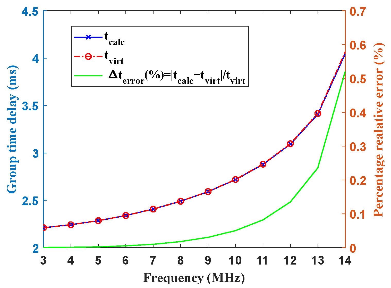
3.2. Validation of the Performance of the Ray-Tracing Algorithm

Due to the fact that the quantities in Equation (6) are obtained using the numerical ray-tracing algorithm, it is necessary to verify the performance of this algorithm. This is carried out to ensure the validity of all values (in Equation (6)). Accordingly, the group time delay is used. In reality, the real measurements of the delay are uncommon, so the calculated group time delay $t_{calc}$ and the virtual time delay $t_{virt}$ are considered. Herein, as long as the time delays mentioned above are both equal, i.e., $t_{virt}=t_{calc}$, the goal is achieved. The propagation theorems, the secant law, and the Breit–Tuve and Martyn propagation equivalent path theorems are involved [32]. However, this work is not the focus of this study; we will not go into detail. If the readers are interested, additional descriptions and details can be found in [27].

As shown in Figure 1, the group time delay and percentage relative error increase with increases in frequency for a fixed elevation angle (30°). Nevertheless, the relative errors are always less than 1%, which is coincident with the results reported in [27]. This small relative error indicates the reliability of the ray-tracing algorithm. On the other hand, we can know that the frequency has an effect on the group time delay, whereas the critical frequency and elevation angle also affect the time delay, which is in line with our general expectations. This mentioned time delay is different from the group delay time in Equation (6), but it is one of the influences on the group delay time. Undoubtedly, the group delay time is affected by frequency, critical frequency, and elevation angles. Next, the variation in numerical ratio between the group delay time and phase advance time as a function of the frequency, critical frequency, and elevation angle are discussed.

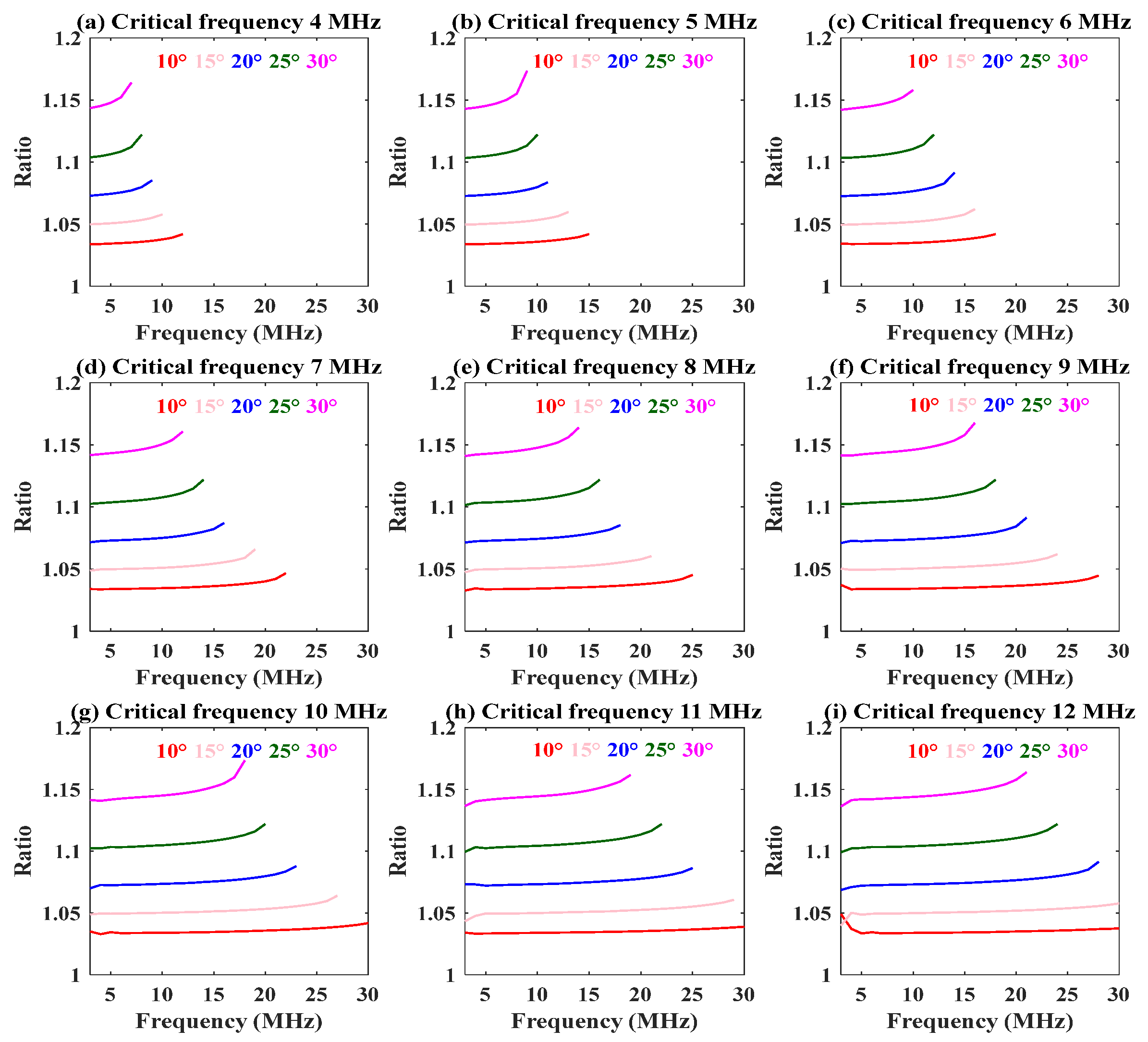
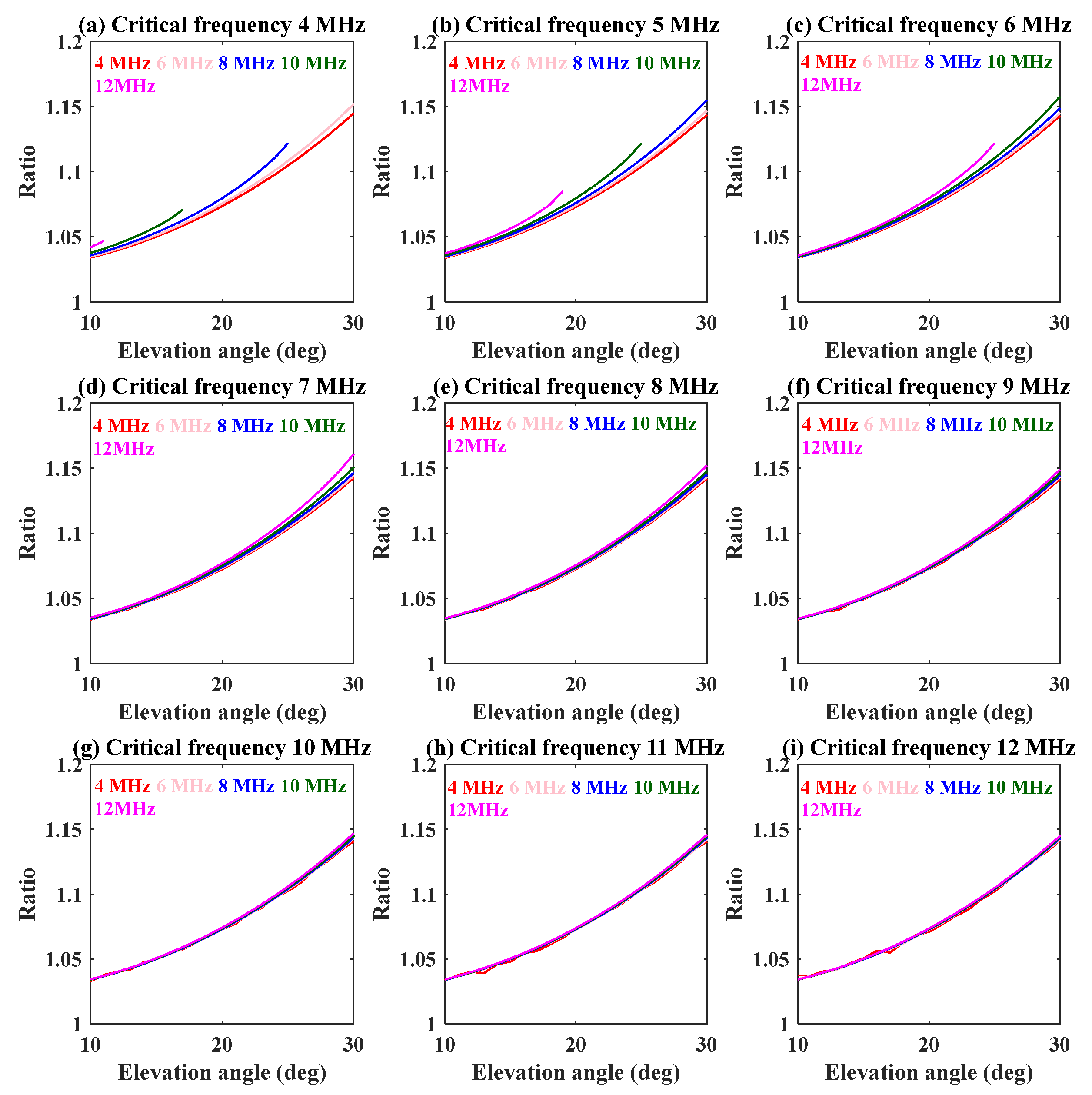
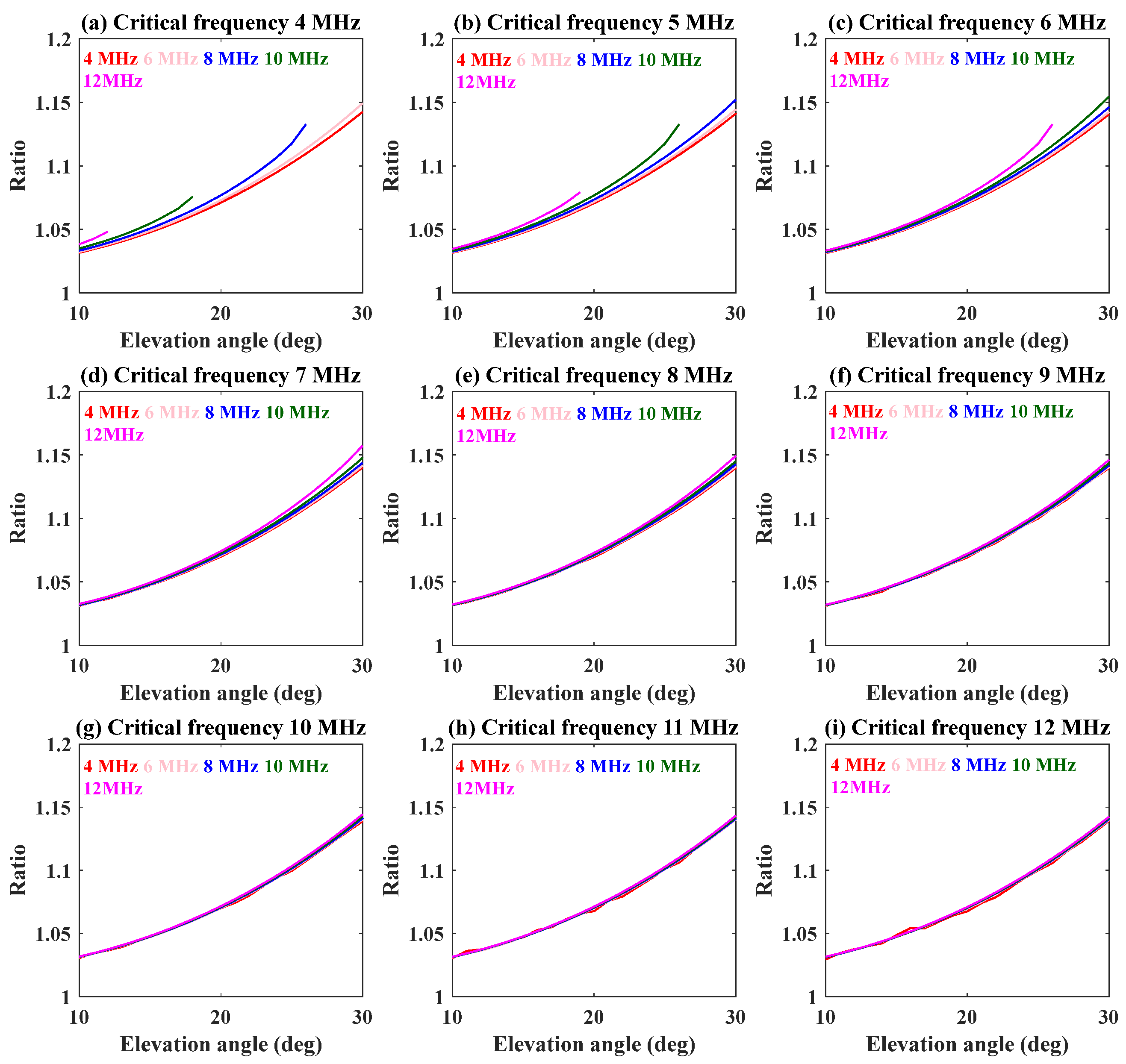
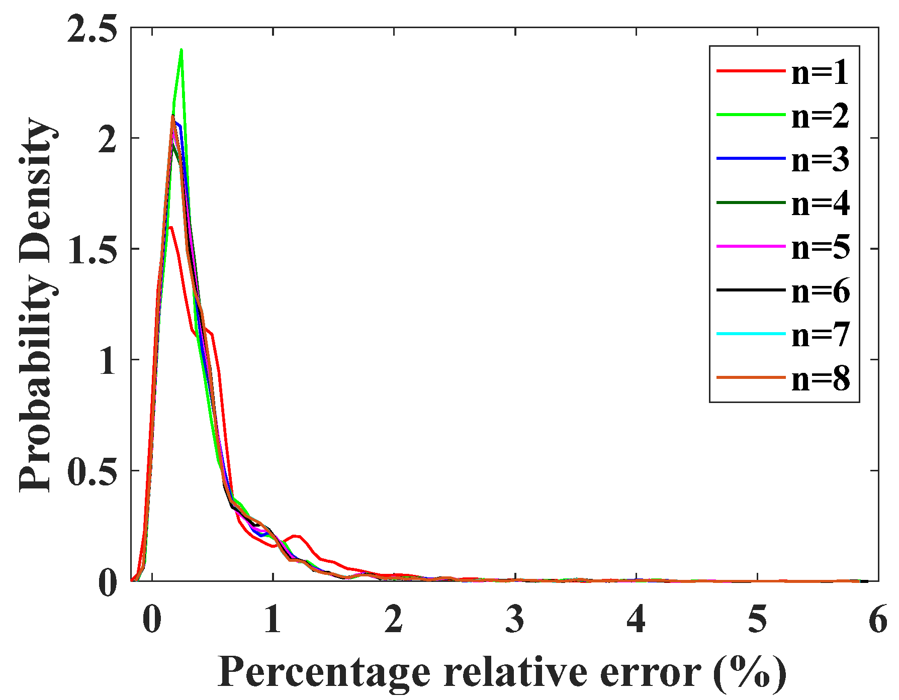
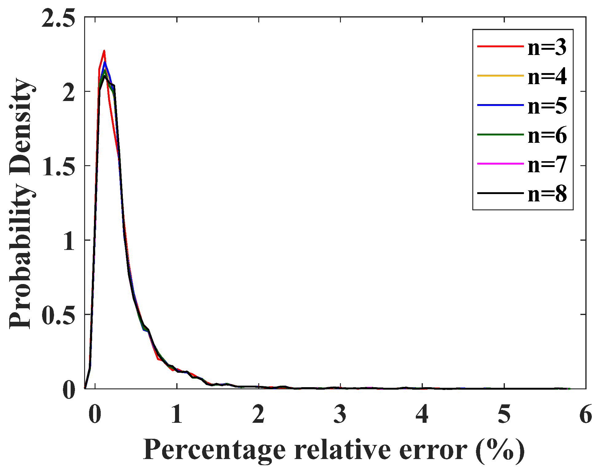
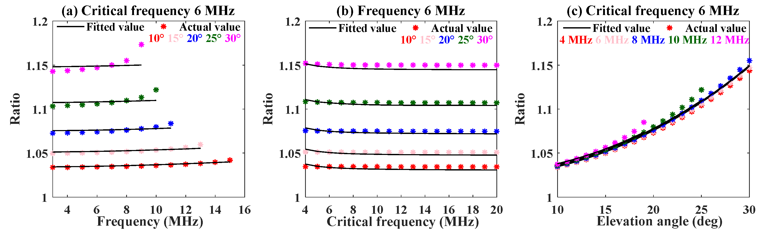
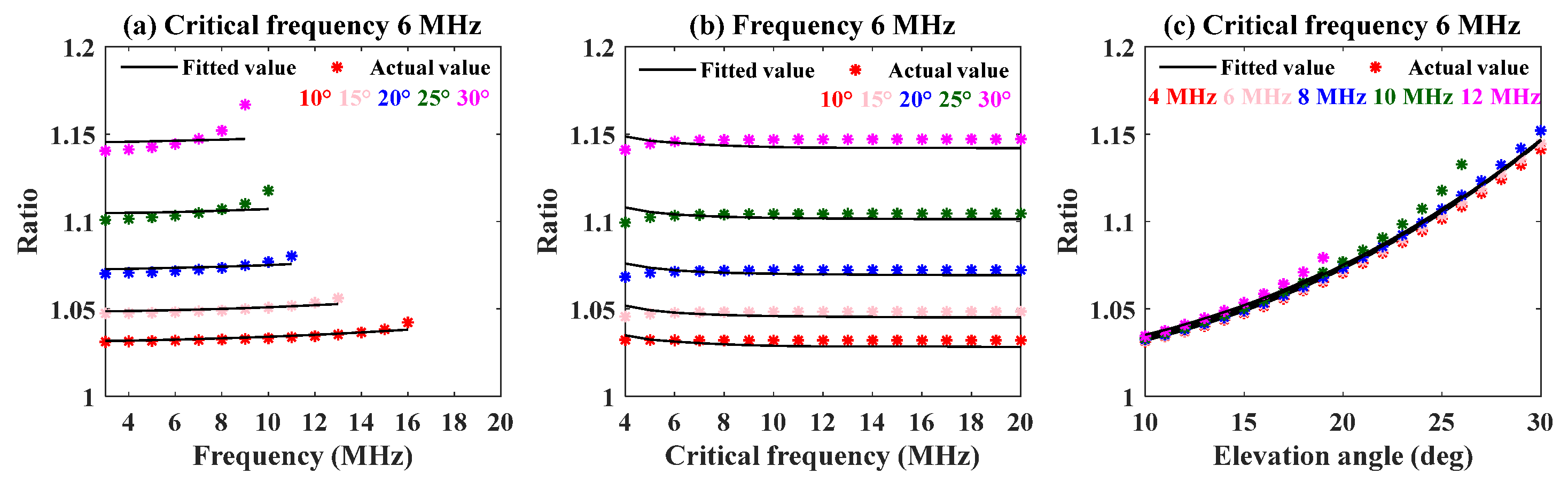
3.3. The Mapping Model between the Numerical Ratio and the Three Factors of Frequency, Critical Frequency, and Elevation Angle

In the following, the trend at the same geocentric base height ($r_b=6540$ km) and semi-thickness height ($y_m=80$ km) is taken as an example to analyze in detail. Considering the propagation distance of the over-the-horizon radar (OTHR), the elevation angles used in this study are all lower than 30° (under one-hop conditions).

The variation in the numerical ratio with radio frequency at different elevation angles (10°–30°) and critical frequencies (4–12 MHz) is shown in Figure 2. The step sizes of the elevation angle and critical frequency are 5° and 1 MHz, respectively. This reveals that the radio frequency has little effect on the numerical ratio. From Figure 3, we know that the numerical ratio hardly changes with the critical frequency. So the numerical ratio is also not influenced by the critical frequency. Combining Figure 2 and Figure 3, we can see that the larger the elevation angle, the greater the numerical ratio.

The trends of the numerical ratio with the elevation angle are exhibited in Figure 4. This figure displays that the numerical ratio increases with increases in the elevation angle. The slope of the curve with the increasing elevation angle remains consistent in each panel of Figure 4. Furthermore, the range of the numerical ratio is from 1 to 1.2.

To summarize, it is assumed that the mapping between the numerical ratio and the three influencing factors is satisfied as follows:

$$y=f_1\left(f,f_c,\beta \right)$$

(8)

where $f_1\left(\right)$ is a function of radio frequency $f$, critical frequency $f_c$, and elevation angle $\beta$; and $y$ is the numerical ratio.

However, from Equation (7), the electron density of the background ionosphere is related to the base height and semi-thickness. Variations in these parameters can affect the propagation path of radio waves. The trends of the numerical ratio with the frequency, critical frequency, and elevation angle at a base height of 6521.2 km are separately shown in Figure 5, Figure 6 and Figure 7. Finally, the conclusions are the same as above.

Further, according to each panel in Figure 8, whether the semi-thickness or base height alters, the trends of the numerical ratio are approximately invariable under most conditions. Thus, the mapping relation of Equation (8) is also applied to other background ionospheric environments. Next, the statistics regression analysis method will be used to investigate the relationship between the numerical ratio and the three factors (frequency, critical frequency, and elevation angle). The specific steps are as below:

First of all, the relationship between the elevation angle and numerical ratio is taken into consideration. Combining the trends in Figure 4 and the integral expressions of the group path and phase path in [33], polynomial fitting is used to describe the relationship with the elevation angle (thereinto, the cosine of the elevation angle is thought of as a whole). Thus, the initial regression model is as follows:

$$y={\displaystyle \sum _{n=0}^{\infty }\frac{a_n}{{\cos }^n\left(\beta \right)}}+{\epsilon }_0$$

(9)

where $\beta$ is the elevation angle, $a_n$ is the coefficient of the polynomial, $n$ is the order of the polynomial, and ${\epsilon }_0$ is a constant term. It is worth underscoring that the addition of higher-order terms can make this equation complicated. Accordingly, the maximum value of the order $n$ is considered to be 8. All data in Figure 2, Figure 3 and Figure 4 are taken as samples and substituted into Equation (9) in turn. The probability density distribution curves of the relative error between the fitted values and actual simulation values for different orders under varying elevation angles are shown in Figure 9. While the order $n$ is greater than 2, the density distributions are similar.

Subsequently, independent variables such as the frequency and critical frequency are added to the regression model. From the definition of the refractive index (Equation (3) in [33]), the orders of the frequency and critical frequency are both quadratic. As shown in the results in Figure 2 and Figure 3, simple linear regression is considered to express the relationship between the numerical ratio and two variables. Thereby, the expression is shown as below:

$$y={\displaystyle \sum _{n=0}^i\frac{a_n}{{\cos }^n\left(\beta \right)}}+{\epsilon }_0+(\frac{b}{f_c^2}+{\epsilon }_1)+(c{f}^2+{\epsilon }_2),3\le i\le 8$$

(10)

where $b$ and $c$ are the coefficients; ${\epsilon }_0$, ${\epsilon }_1$, and ${\epsilon }_2$ are the constant terms; $f_c$ is the critical frequency; and $f$ is the radio frequency.

The probability density distribution curves of the relative error for different orders when there are three independent variables are exhibited in Figure 10. Combining the root mean square errors between the fitted values and the actual simulation values in

Table 1. The root mean square errors between the fitted values and actual simulation values with different orders.

The Order of the Polynomial (n)	Root Mean Square Errors (${10}^{-3}$)
3	6.89594
4	6.88583
5	6.88579
6	6.88434
7	6.88202
8	6.88187

, we observe that no matter how the order varies, their density distributions and root mean square errors have little distinction from each other under the same conditions. So, a mathematical model consisting of any of the order values listed in Table 1 can be used to describe the relationship between the ratio and the three independent variables. In order to reduce the complexity of the model, the third order is chosen. After processing Equation (10), the final regression model can be obtained as follows:

$$y=\frac{a_1}{\cos \left(\beta \right)}+\frac{a_2}{{\cos }^2\left(\beta \right)}+\frac{a_3}{{\cos }^3\left(\beta \right)}+\frac{b}{f_c^2}+c{f}^2+\epsilon$$

(11)

where $a_1$, $a_2$, $a_3$, $b$, and $c$ are the coefficients; and $\epsilon$ is a constant term. Taking all of the data in Figure 2, Figure 3 and Figure 4 into Equation (11) in sequence, the above coefficients can be acquired as $a_1$ = 2.073256, $a_2$ = −0.876382, $a_3$ = 0.18251, $b$ = 0.110992, $c$ = $2.614439\times {10}^{-5}$, and $\epsilon$ = −0.363042 using iterative fitting.

Figure 11 shows that the fitted values derived from the current coefficients and the actual simulation values are almost consistent under different conditions of frequencies, critical frequencies, and elevation angles. In this case, the maximum and minimum relative errors among the fitted values and actual values are 5.66% and $1.8671\times {10}^{-4}$%, respectively. Similarly, all data obtained under another background ionospheric model (Figure 5, Figure 6 and Figure 7, $r_b=6521.2$ km and $y_m=80$ km) are substituted into Equation (11). The corresponding coefficients are $a_1$ = 2.043217, $a_2$ = −0.851211, $a_3$ = 0.1754, $b$ = 0.112767, $c$ = $2.56932\times {10}^{-5}$, and $\epsilon$ = −0.353716. Certainly, the fitted values and actual values can be given as shown in Figure 12. In this scenario, the maximum and minimum relative errors are, respectively, 5.2138% and $1.518\times {10}^{-4}$%. The above results indicate that it is feasible to use Equation (11) to depict the mapping correlation between the numerical ratio and the three factors (frequency, critical frequency, and elevation angle) under different background ionospheric models.

In conclusion, the elevation angle plays an important role in the trend of the numerical ratio between the group delay time and phase advance time. Under different ionospheric models, the relationship between the numerical ratio and the three factors (frequency, critical frequency, and elevation angle) can be described by the same mathematical expression (i.e., Equation (11)).

4. Conclusions

In this study, a ray-tracing algorithm is used to study the trend of the numerical ratio between the group delay time and phase advance time with changes in frequency, critical frequency, and elevation angle associated with the Quasi-parabolic model. The simulations reveal that the numerical ratio is mainly determined by the elevation angle, while the frequency and critical frequency have little effect. The range of the numerical ratio is from 1 to 1.2. In addition, the mathematical model of the numerical ratio with respect to frequency, critical frequency, and elevation angle is established using the regression analysis method. The model coefficients are given via iterative fitting. On the other hand, the relativity between the ratio and the three factors of frequency, critical frequency, and elevation angle is confirmed by the little relative errors between the fitting values and simulation values under the different background ionospheric models. This study provides a novel idea and method for researching ionosphere-induced group delay and phase advance, which aids in developing a more reliable and stable short-wave communication system.

References

1. Xiong, N.L.; Tang, C.C.; Li, X.J. Introduction to Ionospheric Physics; Wuhan University Press: Wuhan, China, 1999; ISBN 7-307-02672-4. (In Chinese) [Google Scholar]
2. Wen, D.B. Investigation of GPS-Based Ionospheric Tomographic Algorithms and Their Applications. Ph.D. Thesis, Institute of Geodesy and Geophysics Chinese Academy of Sciences, Wuhan, China, 2007. [Google Scholar]
3. Heelis, R.A.; Maute, A. Challenges to Understanding the Earth’s Ionosphere and Thermosphere. JGR Space Phys. 2020, 125, e2019JA027497. [Google Scholar] [CrossRef]
4. Klobuchar, J.A. Ionospheric Effects on GPS. Glob. Position. Syst. Theory Appl. 1991, 1, 517–546. [Google Scholar] [CrossRef]
5. Xiao, Z.B.; Liu, Z.Y.; Tang, X.M.; Wang, F.X. Effect of ionosphere dispersion on the navigation signal receiving. J. Natl. Univ. Def. Technol. 2014, 36, 146–149. [Google Scholar] [CrossRef]
6. Klobuchar, J. Ionospheric Time-Delay Algorithm for Single-Frequency GPS Users. IEEE Trans. Aerosp. Electron. Syst. 1987, 23, 325–331. [Google Scholar] [CrossRef]
7. Prieto-Cerdeira, R.; Orús Pérez, R.; Breeuwer, E.; Lucas-Rodriguez, R.; Falcone, M. Performance of the Galileo Single-Frequency Ionospheric Correction During In-Orbit Validation. GPSworld 2014, 25, 53–58. [Google Scholar]
8. Yuan, Y.; Wang, N.; Li, Z.; Huo, X. The BeiDou Global Broadcast Ionospheric Delay Correction Model (BDGIM) and Its Preliminary Performance Evaluation Results. Navigation 2019, 66, 55–69. [Google Scholar] [CrossRef]
9. Pang, J.; Liu, Z.Y.; Tang, X.M.; Ou, G. Ionosphere dispersion effects simulation for high order BOC modulated signals. J. Natl. Univ. Def. Technol. 2015, 37, 74–77. [Google Scholar] [CrossRef]
10. Liu, X.; Yuan, Y.; Huo, X.; Li, Z.; Li, W. Model Analysis Method (MAM) on the Effect of the Second-Order Ionospheric Delay on GPS Positioning Solution. Chin. Sci. Bull. 2010, 55, 1529–1534. [Google Scholar] [CrossRef]
11. Zhang, J.; Gao, J.; Yu, B.; Sheng, C.; Gan, X. Research on Remote GPS Common-View Precise Time Transfer Based on Different Ionosphere Disturbances. Sensors 2020, 20, 2290. [Google Scholar] [CrossRef] [PubMed]
12. Petrie, E.J.; Hernández-Pajares, M.; Spalla, P.; Moore, P.; King, M.A. A Review of Higher Order Ionospheric Refraction Effects on Dual Frequency GPS. Surv. Geophys. 2011, 32, 197–253. [Google Scholar] [CrossRef]
13. Hernández-Pajares, M.; Aragón-Ángel, À.; Defraigne, P.; Bergeot, N.; Prieto-Cerdeira, R.; García-Rigo, A. Distribution and Mitigation of Higher-order Ionospheric Effects on Precise GNSS Processing. JGR Solid Earth 2014, 119, 3823–3837. [Google Scholar] [CrossRef]
14. Zhang, X.; Ren, X.; Guo, F. Influence of Higher-Order Ionospheric Delay Correction on Static Precise Point Positioning. Geomat. Inf. Sci. Wuhan Univ. 2013, 38, 883–887. [Google Scholar] [CrossRef]
15. Cai, C.; Liu, G.; Yi, Z.; Cui, X.; Kuang, C. Effect Analysis of Higher-Order Ionospheric Corrections on Quad-Constellation GNSS PPP. Meas. Sci. Technol. 2019, 30, 024001. [Google Scholar] [CrossRef]
16. Hadas, T.; Krypiak-Gregorczyk, A.; Hernández-Pajares, M.; Kaplon, J.; Paziewski, J.; Wielgosz, P.; Garcia-Rigo, A.; Kazmierski, K.; Sosnica, K.; Kwasniak, D.; et al. Impact and Implementation of Higher-Order Ionospheric Effects on Precise GNSS Applications. JGR Solid Earth 2017, 122, 9420–9436. [Google Scholar] [CrossRef]
17. Jin, S.; Jin, R.; Kutoglu, H. Positive and Negative Ionospheric Responses to the March 2015 Geomagnetic Storm from BDS Observations. J. Geod. 2017, 91, 613–626. [Google Scholar] [CrossRef]
18. Chen, L.; Yi, W.; Song, W.; Shi, C.; Lou, Y.; Cao, C. Evaluation of Three Ionospheric Delay Computation Methods for Ground-Based GNSS Receivers. GPS Solut. 2018, 22, 125. [Google Scholar] [CrossRef]
19. Hartmann, G.K.; Leitinger, R. Range Errors Due to Ionospheric and Tropospheric Effects for Signal Frequencies above 100 MHz. Bull. Geod. 1984, 58, 109–136. [Google Scholar] [CrossRef]
20. Brunner, F.K.; Gu, M. An Improved Model for the Dual Frequency Ionospheric Correction of GPS Observations. Manuscripta Geod. 1991, 16, 205–214. [Google Scholar]
21. Bassiri, S.; Hajj, G.A. Higher-Order Ionospheric Effects on the GPS Observables and Means of Modeling Them. Manuscripta Geod. 1993, 18, 280–289. [Google Scholar]
22. Strangeways, H.J.; Ioannides, R.T. Rigorous Calculation of Ionospheric Effects on GPS Earth-Satellite Paths Using a Precise Path Determination Method. AGeod 2002, 37, 281–292. [Google Scholar] [CrossRef]
23. Wang, K.N.; Fu, H.Y. Simulation of the ionospheric higher-order effect and Doppler effect during TID based on ray tracing. Chin. J. Radio Sci. 2022, 37, 1032–1038. [Google Scholar] [CrossRef]
24. Su, K.; Jin, S.; Hoque, M. Evaluation of Ionospheric Delay Effects on Multi-GNSS Positioning Performance. Remote Sens. 2019, 11, 171. [Google Scholar] [CrossRef]
25. Liu, Z.; Yang, Z. Anomalies in Broadcast Ionospheric Coefficients Recorded by GPS Receivers over the Past Two Solar Cycles (1992–2013); Springer: New York, NY, USA, 2016. [Google Scholar] [CrossRef]
26. Wang, A.; Chen, J.; Zhang, Y.; Meng, L.; Wang, J. Performance of Selected Ionospheric Models in Multi-Global Navigation Satellite System Single-Frequency Positioning over China. Remote Sens. 2019, 11, 2070. [Google Scholar] [CrossRef]
27. Bianchi, C.; Settimi, A.; Scotto, C.; Azzarone, A.; Lozito, A. A Method to Test HF Ray Tracing Algorithm in the Ionosphere by Means of the Virtual Time Delay. Adv. Space Res. 2011, 48, 1600–1605. [Google Scholar] [CrossRef]
28. Budden, K.G. The Propagation of Radio Waves: The Theory of Radio Waves of Low Power in the Ionosphere and Magnetosphere, 1st ed.; Cambridge University Press: Cambridge, UK, 1985; ISBN 978-0-521-25461-8. [Google Scholar]
29. Davies, K. Ionospheric Radio; The Institution of Engineering and Technology: London, UK, 1990. [Google Scholar]
30. Rawer, K. Wave Propagation in the Ionosphere; Springer: Dordrecht, The Netherlands, 1993; ISBN 978-90-481-4069-5. [Google Scholar]
31. De Voogt, A. The Calculation of the Path of a Radio-Ray in a Given Ionosphere. Proc. IRE 1953, 41, 1183–1186. [Google Scholar] [CrossRef]
32. Pietrella, M.; Pezzopane, M.; Pignatelli, A.; Pignalberi, A.; Settimi, A. An Updating of the IONORT Tool to Perform a High-Frequency Ionospheric Ray Tracing. Remote Sens. 2023, 15, 5111. [Google Scholar] [CrossRef]
33. Croft, T.A.; Hoogansian, H. Exact Ray Calculations in a Quasi-Parabolic Ionosphere with No Magnetic Field. Radio Sci. 1968, 3, 69–74. [Google Scholar] [CrossRef]
Figure 1. Variation in the time delay and percentage relative error with radio frequency for the elevation angle of 30°. The blue curve shows the calculated group time delay, the red curve shows the virtual group time delay, and the green curve shows the percentage relative errors.
Remotesensing 16 00553 g001
Figure 2. Variation in numerical ratio with the radio frequency at different elevation angles (5–30°, step size of 5°). Each panel shows the trends calculated at different critical frequencies (4–12 MHz, step size of 1 MHz).
Remotesensing 16 00553 g002
Figure 3. Variation in numerical ratio with the ionospheric critical frequency at different elevation angles. Each panel shows the trends calculated at different frequencies (4–20 MHz; the step size is 2 MHz).
Remotesensing 16 00553 g003
Figure 4. Variation in numerical ratio with the elevation angle at different frequencies. Each panel shows the trends calculated at different critical frequencies (4–12 MHz; the step size is 1 MHz).
Remotesensing 16 00553 g004
Figure 5. Variation in numerical ratio with the radio frequency at different elevation angles under another ionospheric model. Each panel shows the trends calculated at different critical frequencies.
Remotesensing 16 00553 g005
Figure 6. Variation in numerical ratio with the ionospheric critical frequency at different elevation angles under another ionospheric model. Each panel shows the trends calculated at different frequencies.
Remotesensing 16 00553 g006
Figure 7. Variation in numerical ratio with the elevation angle at different frequencies under another ionospheric model. Each panel shows the trends calculated at different critical frequencies.
Remotesensing 16 00553 g007
Figure 8. Numerical ratio profiles as a function of different parameters for a range of conditions. Each column corresponds to Figure 2, Figure 3 and Figure 4, respectively. The top panels show the trends calculated at the different semi-thicknesses and the bottom panels show the trends at the different base heights.
Remotesensing 16 00553 g008
Figure 9. Probability density of the percentage relative error between the fitted values and actual simulation values for different orders in the case of one independent variable (i.e., elevation angle).
Remotesensing 16 00553 g009
Figure 10. Probability density of the percentage relative error between the fitted values and actual simulation values for different orders in the case of three independent variables (i.e., frequency, critical frequency, and elevation angle).
Remotesensing 16 00553 g010
Figure 11. (a) Fitted value and actual value profiles as a function of radio frequency at different elevation angles; (b) fitted value and actual value profiles as a function of critical frequency at different elevation angles; and (c) fitted value and actual value profiles as a function of elevation angles at different frequencies. The asterisks refer to the actual results, and the black solid lines refer to the fitted results.
Remotesensing 16 00553 g011
Figure 12. Under another ionospheric model, (a) fitted value and actual value profiles as a function of radio frequency at different elevation angles; (b) fitted value and actual value profiles as a function of critical frequency at different elevation angles; and (c) fitted value and actual value profiles as a function of elevation angles at different frequencies. The asterisks refer to actual results, and the black solid line refers to fitted results.
Remotesensing 16 00553 g012