Article

Research on Methods to Improve Length of Day Precision by Combining with Effective Angular Momentum

1
National Time Service Center, Chinese Academy of Sciences, Xi’an 710600, China
2
School of Electronic, Electrical and Communication Engineering, University of Chinese Academy of Sciences, Beijing 100049, China
3
Key Laboratory of Time Reference and Applications, Chinese Academy of Sciences, Xi’an 710600, China
4
School of Astronomy and Space Science, University of Chinese Academy of Sciences, Beijing 100049, China
5
School of Engineering and Technology, Chengdu University of Technology, Leshan 614000, China
*
Author to whom correspondence should be addressed.
Remote Sens. 2024, 16(4), 722; https://doi.org/10.3390/rs16040722
Submission received: 9 January 2024 / Revised: 13 February 2024 / Accepted: 15 February 2024 / Published: 19 February 2024

Abstract

:
Due to the high correlation between Effective Angular Momentum (EAM) and Length of Day (LOD) data, and the wide application of LOD prediction, this study proposes to combine EAM data with Global Navigation Satellite System (GNSS) LOD data to obtain a more accurate LOD series and attempt to provide a reasonable formal error for the EAM dataset. Firstly, tidal corrections are applied to the LOD data. A first-order difference method is proposed to identify outliers in GNSS LODR (tidal corrected LOD) data, and the EAM data are converted into LODR data using the Liouville equation. Then, the residual term and the fitted term are obtained by least squares fitting. Finally, the fitted residual terms of GNSS LODR and EAM LODR are combined by using the Kalman combination method. In this study, EAM data from the German Research Centre for Geosciences (GFZ) (2019–2022), as well as LOD data from Wuhan University (WHU) and Jet Propulsion Laboratory (JPL), are used for the Kalman combination algorithm experiment. In the Kalman combination, we consider weighted combination based on formal error. However, none of the computing centers provide an uncertainty estimation for the EAM dataset. Therefore, we simulate the combination experiment of LOD and EAM with formal error ranging from 0 to 100 us. The experiment shows that using reasonable formal error for the EAM dataset can improve the accuracy of LOD. Finally, when the formal error of EAM is 2–5 times that of the GNSS LOD formal error, i.e., the EAM formal error is between 10 and 30 us, the accuracy of the combined LOD can be improved by 10–20%.
Keywords:
LOD; EAM; GNSS; LS; Kalman

1. Introduction

Due to various physical factors such as the Earth’s interior, surface, and space, the Earth’s rotation rate varies at a time scale of several days to several years. These variations are typically characterized by changes in the Length of Day (LOD), which reflects the changes in the Earth’s rotation rate. LOD, along with polar motion, constitutes the Earth Rotation Parameters (ERPs) [1,2,3]. High-precision ERPs play a crucial role in fields such as deep space exploration, satellite navigation, and the establishment and maintenance of reference frames [4,5,6].
Global Navigation Satellite System (GNSS) [7,8], Very Long Baseline Interferometry (VLBI) [9,10], Satellite Laser Ranging (SLR) [11], Lunar Laser Ranging (LLR) [12], and Doppler Orbitography and Radiopositioning Integrated by Satellite (DORIS) [13,14] can be used to measure ERPs, such as LOD. Among these techniques, GNSS has a global network of observation stations, enabling continuous monitoring and fast data processing [5,6]. The International Earth Rotation and Reference Systems Service (IERS) is the most authoritative organization that provides ERP data. Their final products integrate measurement results from various space geodetic techniques. However, the final products may have a low timeliness and are generally used for product comparison and analysis [15,16].
At interannual or shorter time scales, Atmospheric Angular Momentum (AAM) is considered to be the primary factor contributing to variations in LOD [17,18]. Rosen and Salstein [18] demonstrated that AAM accounts for 90% of LOD variations at seasonal and shorter time scales. Gross et al. [19] demonstrated that AAM explains 85.8% of the LOD variations on interannual time scales. Rekier et a1. [20] analyzed the LOD data of IERS EOP C04 series and the total geophysical angular momentum data of AAM, Oceanic Angular Momentum (OAM), and Hydrological Angular Momentum (HAM), and explained the correlation between LOD and angular momentum.
Dickey et al. [21] found that at shorter time scales, the signal-to-noise ratio of AAM is superior to that of LOD, suggesting that AAM data may provide a better indication of high-frequency variations in LOD compared to geodetic measurements. Freedman et al. [22], through an analysis of the periodicity and power spectra of AAM and LOD, discovered a high degree of consistency between the two variables. They proposed that in the absence of geodetic data, AAM is both a reasonable proxy and useful supplement to geodetically derived LODs even for high-frequency fluctuations.
Research has shown that the use of AAM and other data can improve the prediction accuracy of Universal time (UT1) and LOD. Johnson et al. [23] demonstrated that the utilization of AAM data can enhance the short-term prediction accuracy of UT1 and LOD. Dill and Dobslaw [24] incorporated AAM, OAM, and HAM data into the prediction of UT1 and LOD, leading to a significant improvement in the prediction accuracy. Furthermore, Dill et al. [25] introduced Sea-Level Angular effective Momentum (SLAM) data and constructed Effective Angular Momentum (EAM) data (EAM = AAM + OAM + HAM + SLAM), which notably enhanced the short-term prediction accuracy of UT1 and LOD within 1–6 days. With the improvement in the accuracy of the EAM dataset, the IERS has begun utilizing AAM data to assist in their daily Earth Orientation Parameter (EOP) prediction products.
Li et al. [26] proposed a UT1/LOD prediction method based on a denoised EAM dataset. By improving the prediction accuracy of UT1/LOD, it was demonstrated that combining the least squares fitting residuals of the C04 LODR (tidal-corrected LOD) and EAM LODR can enhance the accuracy of EAM LODR. Building upon the work of Li et al. [26], this study combines GNSS LODR with EAM LODR to simultaneously improve the accuracy of EAM and LODR. Additionally, an attempt is made to provide the formal error of EAM.
In this paper, the following steps were taken. Firstly, the GNSS LOD sequence was examined and outliers were detected and removed using a first-order difference method. The outliers were replaced with a weighted average of the preceding and succeeding values. Then, a least squares algorithm was used to fit the derived LODR dataset from EAM and the tidal-corrected GNSS LODR. The residuals obtained from the fitting were subjected to Kalman filtering. The processed residual terms were combined and ultimately merged with the fitted terms to obtain the combined LODR sequence. During the combination process, simulations were conducted to assess the combination’s effectiveness under different formal EAM errors, and a reasonable formal EAM error was determined. The second section of this article provides a brief description of the dataset used. Section 3 outlines the data processing workflow, including tidal correction, EAM data analysis, outlier removal, least squares fitting, Kalman filtering, and combination algorithms. Section 4 simulates the formal error of EAM and studies its contribution to the combination with LOD. Section 5 evaluates the combined effect of different GNSS analysis organization LOD datasets and EAM using measured datasets. Section 6 discusses the rationality of the algorithm in detail, including the correlation analysis between GNSS LOD formal error and accuracy. Section 7 presents the main research findings of this article.

2. Data Set

2.1. LOD Dataset

This article analyzes the LOD products of two GNSS institutions, Wuhan University (WHU) and the Jet Propulsion Laboratory (JPL). WHU serves as the data analysis center for the International GNSS Monitoring and Assessment System (iGMAS) and the International GNSS Service (IGS), while JPL serves as the data analysis center for IGS. In the subsequent sections of this article, the WHU/JPL LOD dataset spanning from January 2019 to December 2022, a total of 4 years, is used for algorithm verification. The precise C04 LOD dataset is used for result comparison and analysis.

2.2. EAM Dataset

The EAM function is composed of the Z-components of AAM, OAM, HAM, and SLAM, which are combined together. The modeling process of OAM and the calculation method of HAM are described in detail by Jungclaus et al. [27] and Dill [28]. The calculation processes of AAM and SLAM are explained in detail in the literature by Dobslaw and Dill [29], Tamisiea et al. [30], and Hageman and Dumenil [31]. The datasets of AAM, OAM, HAM, SLAM, and others are provided by the German Research Centre for Geosciences (GFZ). The website for accessing these datasets is http://esmdata.gfz-potsdam.de:8080 (accessed on 1 December 2023) [31].
Due to the inconsistent sampling intervals of AAM, OAM, HAM, and SLAM data, as shown in Table 1, a weighted approach was used to convert the 3 h sampling interval to a 24 h sampling interval. The four components were then added together to form the EAM dataset. In constructing the EAM, this study refers to Dill et al. [25].

3. Methods

3.1. LOD Tidal Correction

This article first applies the experience model provided by the IERS protocol to correct tidal variations in the LOD products of WHU and JPL [1]. This correction results in an LODR sequence that removes tidal components.

3.2. EAM Data Analysis

According to the Liouville equation,
Ψ = Ω 2 π dUT 1 R d t
LODR is derived by
LODR = 2 π Ω Ψ
where, Ψ is the angular momentum, and Ω is the average angular velocity of the Earth 7.292115 × 10⁻⁵ rad s−1. The above formula allows conversion between LODR and GAM. In this article, the AAM, OAM, HAM, and SLAM datasets from January 2019 to December 2022, a total of 4 years, were combined into EAM using the method shown in Section 2.2. Based on the Liouville equation, EAM was then converted into LODR and compared with the IERS 14C04 LODR series. The comparison is shown in Figure 1.
The strength of the correlation between the LODR derived from EAM (EAM LODR) and the C04 LODR can be represented using the Pearson correlation coefficient, as shown in Figure 2. According to Equation (3), the Pearson correlation coefficient between two continuous variables (X and Y) is obtained by dividing their covariance by the product of their respective standard deviations.
ρ x , y = c o v ( X , Y ) σ X σ Y

3.3. GNSS LODR Outlier Removal

The LODR data for WHU and JPL from January 2019 to December 2022 were compared with the LODR data from IERS C04, as shown in Figure 3.
From the bottom panel in Figure 3, it can be observed that the difference between WHU and C04 is relatively stable with smaller fluctuations. On the other hand, the difference between JPL and C04 shows larger fluctuations and exhibits noticeable periodicity. In particular, there is an outlier point of approximately 200 us for WHU around December 2019. Considering the data’s stationarity and the data themselves, without relying on external data, a first-order difference method is proposed for outlier detection. The first-order difference in LODR between WHU and C04 is shown in Figure 4.
From Figure 4, it can be observed that the first-order difference in C04 LODR, represented by the red line, appears to be more stable without any outlier points. On the other hand, the first-order difference in WHU LODR, represented by the black line, shows an outlier point that coincides with the outlier point in the difference between WHU LODR and C04 LODR. By using the first-order difference method, the outlier points in WHU LODR can be accurately removed. When removing outlier points, a weighted average of the data before and after the outlier point is used to replace the removed outlier point, ensuring the continuity of the data.

3.4. Least Squares Fitting

The LODR sequence mainly consists of the long-term trend term, semi-annual term, annual term, and irregular variation term. The trend term and periodic terms are fitted using the least squares method, according to the following formula:
f L O D R ( t ) = a 0 + a 1 t + Σ i = 1 n c i sin ( 2 π t T i ) + d i cos ( 2 π t T i )
where, a 0 and a 1 represent the parameters of the linear trend component, c i and d i represent the parameters of the periodic component, T i represents the length of the periodic cycle, and n represents the number of cycles. Here, n is set to 8, and the values of T i correspond to 9.13, 13.7, 27.4, 121.75, 182.62, 365.24, 1095.72, and 3396.73 days [25,32,33,34].
Figure 5 from top to bottom represents the LODR data, least squares fitting, and residual of the fitting for the C04, WHU, JPL, and EAM datasets, respectively. It can be observed that there is a significant deviation between the EAM LODR data and the C04 LODR data. However, the residuals of the least squares fitting for both datasets are almost identical, and the Pearson correlation coefficient between the residuals of the two fits is as high as 0.9876. This finding suggests that although there is a noticeable discrepancy between the EAM and C04 LODR data, their respective least squares fits exhibit similar patterns of residual error. The high Pearson correlation coefficient indicates a strong linear relationship between the residual error of the two fits.

3.5. Kalman Filtering and Combination

The LODR least squares fitting residuals for EAM, WHU, and JPL can be processed using Kalman filtering for noise reduction. Kalman filtering is an optimal linear filter based on the minimum mean square error criteria. It only requires the previous estimate and the current observation to calculate the current estimate [35,36,37,38]. The state equation and observation equation for Kalman filtering are as follows:
x k = F k x k 1 + w k z k = H k x k + v k
The prediction equation and the correction equation are as follows:
x k / k 1 = F k x k 1 / k 1 x k / k = x k / k 1 + K k ( z k H k x k / k 1 )
The Kalman gain and covariance matrix are as follows:
K k = P k / k 1 H k T / ( H k P k / k 1 H k T + R k )
P k / k 1 = F k P k 1 / k 1 F k T + Q k P k / k = ( 1 K k H k ) P k / k 1
As can be seen in Figure 6, after filtering, the difference between the residuals of EAM LODR (least squares fitting residuals) and C04 LODR (least squares fitting residuals) is smaller. In other words, the black line in the lower figure is more stable with smaller fluctuations compared to the red line.
The Kalman combination algorithm is used to combine the least squares fitting residuals of EAM LODR with those of WHU/JPLLODR. There are errors present in the least squares fitting residuals of EAM, WHU/JPL, and C04. Therefore, by applying the Kalman algorithm to combine the least squares fitting residuals of EAM LODR with those of WHU/JPL LODR, we can obtain a combined value that is closest to the least squares fitting residuals of C04. This can, in turn, improve the LODR accuracy of WHU/JPL. The formula is as follows:
Z = Z 1 + A × ( Z 2 Z 1 )
Z1 represents the least squares fitting residuals of EAM LODR, and Z2 represents the least squares fitting residuals of WHU/JPL LODR. By calculating the weight of their combination using the formal error, denoted as A (A = the formal error of EAM LODR/(the formal error of EAM LODR+ the formal error of WHU/JPL LODR)), the optimal combined value Z can be obtained.

4. Simulation Experiment of EAM Formal Error

Currently, there is no institution that has released the numerical values and distribution of the formal error or uncertainties associated with AAM, OAM, HAM, and SLAM. However, relevant research has been conducted by Rosen et al. [39], Gross and Eubanks [40], Bell et al. [41], and Gross et al. [42] to evaluate the error present in AAM data. In constructing a Kalman filter, Freedman et al. [22] selected 50 us as the formal error for AAM analysis and prediction sequences. Based on the above analysis, we have chosen a range of 0–100 us as the formal error for EAM and conducted combined simulation experiments.

4.1. WHU and EAM Simulation Combination Experiment

The LODR products of WHU from January 2019 to December 2022 were used for LOD combination experiments with EAM under different formal error. In the combination experiment, the formal error of EAM and WHU LODR is taken as the weight of the combination, and the precision of the combined LODR is compared with that of C04 LODR. The combination result is shown in Figure 7.
Based on Figure 7, we can observe that when the formal accuracy of EAM is much lower than that of WHU, the combined LODR precision is lower. As the formal error of EAM increases, the combined LODR precision gradually converges to the LODR precision of WHU. This can be understood as when the formal accuracy of EAM is much lower than that of WHU, it indicates that the proportion of EAM in the combination approaches 1. On the other hand, when the formal accuracy of EAM is much higher than that of WHU, it indicates that the proportion of EAM in the combination approaches zero. When the ratio of formal accuracy between EAM and WHU is 3–5 times, i.e., the formal accuracy of EAM is between 4 and 10 us, it can result in a higher combined LODR precision (WHU’s formal accuracy is 1.16 us).

4.2. JPL and EAM Simulation Combination Experiment

The LODR products of JPL from January 2019 to December 2022 were used for LOD combination experiments with EAM under different formal errors. In the combination experiment, the formal errors of EAM and JPL LODR are taken as the weight of the combination, and the precision of the combined LODR is compared with that of C04 LODR. The combination result is shown in Figure 8.
In Figure 8, similar conclusions were also obtained as in Figure 7. As the magnitude of EAM’s formal error increases, the combined LODR gradually converges to the accuracy of JPL LODR. When the ratio of formal accuracy between EAM and JPL is of 2.5–5 times, i.e., the formal accuracy of EAM is between 15 and 30 us, it can result in a higher combined LODR precision (JPL’s formal accuracy is 6.32 us).

4.3. iGMAS and EAM Simulation Combination Experiment

To further validate the formal error of EAM, an LOD combination experiment was conducted using the iGMAS LODR products from January 2019 to December 2022, along with EAM incorporating various levels of formal error. The combination result is shown in Figure 9.
Similar findings to Figure 7 were observed in Figure 9, showing a gradual convergence of the combined LODR towards the precision of iGMAS LODR as the formal error of EAM increased. When the ratio of formal accuracy between EAM and iGMAS is 2–4 times, i.e., the formal accuracy of EAM is between 10 and 30 us, it can result in a higher combined LODR precision (iGMAS formal accuracy at 7.20 us).

5. Combination of Measured Datasets

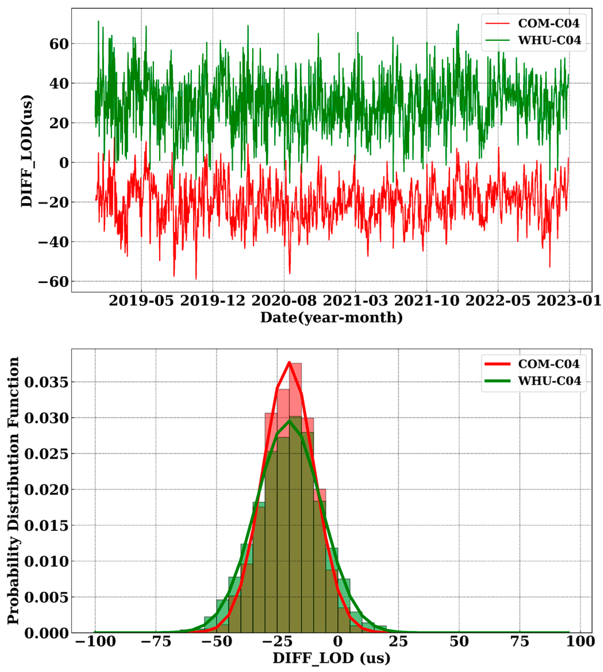
5.1. Combination of WHU with EAM

When using the LOD products of WHU from Janurary 2019 to Decemeber 2022, the tidal term was deducted according to the IERS agreement to obtain the LODR data. The first-order differencing method was applied to identify and fill in outliers. An EAM sequence was constructed using the method described in Section 2.2. The EAM sequence was converted to EAM LODR using the Liuville equation. A least square fitting was performed on both WHU LODR and EAM LODR to obtain the residual terms and the fitted terms. Kalman filtering was applied separately to the residual terms to reduce noise, and then Kalman combination was performed on the denoised residual terms. Finally, the combined residual terms were added to the fitted terms of WHU LODR to obtain the combined WHU LODR. During the combination process, the ratio between the formal error of EAM and that of WHU is 4.3, i.e., the formal error of EAM is 5 us. The final combined WHU LODR was compared and analyzed with C04 LODR. The combination result is shown in Figure 10.
In Table 2, the column “COM” means the combination of WHU LODR and EAM LODR. The curve fitting in Figure 10 and the histogram clearly show that the peak value of the WHU LODR combination is higher, the convergence is better, and the distribution is more concentrated compared to the combination before. Table 2 provides a statistical analysis of the difference between WHU before and after combination with C04 LOD. Before the combination, the precision of the WHU LOD is 13.51 us, and after the combination, it is 10.57 us, resulting in a precision improvement of 21.76%. Additionally, the mean and extreme values have also been improved after the combination. It should be noted that the comparison results in this section are slightly different from those in Section 4.1. This is because in Section 4.1, the WHU is interpolated to the zero moment (UTC 00:00) of EOP 14 C04 for comparison, while in this section, the EOP 14 C04 is interpolated to the noon moment (UTC 12:00) of WHU for comparison.

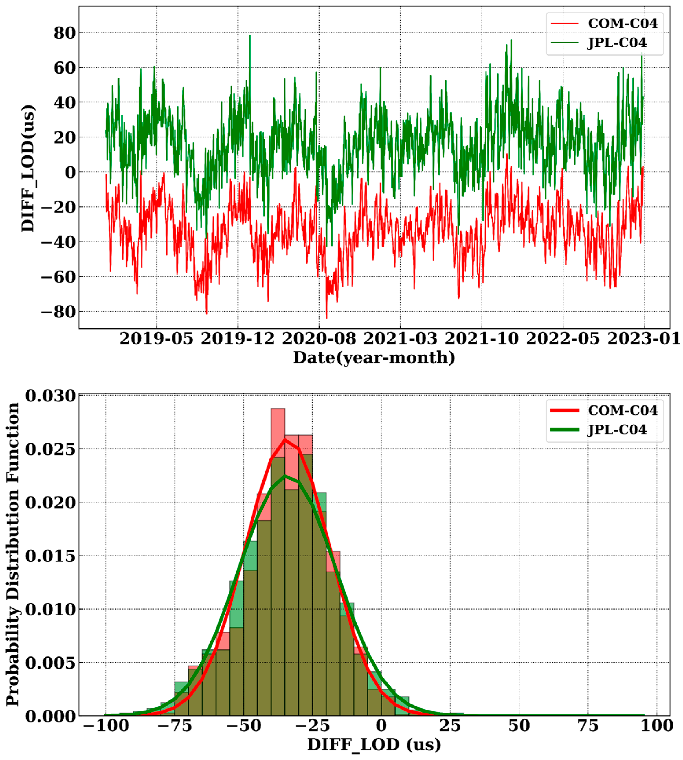
5.2. Combination of JPL with EAM

Using least squares fitting, the JPL LODR and EAM LODR from January 2019 to December 2022 were fitted. The residuals and fitted values were obtained. The residuals were then separately filtered using Kalman filtering to reduce noise. After that, the filtered residuals were combined using Kalman fusion. Finally, the combined residuals were added to the JPL LODR fitted values to form the combined JPL LODR. During the combination process, the ratio of the formal error between EAM and JPL is 3.8, i.e., the formal error of the EAM is 24 us. The final combined JPL LODR was compared and analyzed with the C04 LODR. In Table 3, the column “COM” means the combination of JPL LODR and EAM LODR.
Figure 11 shows the curve fitting and histogram, indicating that the combined JPL LODR has higher and more concentrated peaks compared to before combination. Table 3 presents the statistical analysis of the differences between JPL LODR before and after combination with C04 LODR. The accuracy of JPL LODR before combination is 17.75 us, while after combination, it improves to 15.42 us, showing a precision improvement of 13.35%. The mean, median, and extreme values are all improved after combination. It is important to note that the results of this section slightly differ from Section 4.2. This is because Section 4.2 compares JPL interpolated to the zero-epoch moment (UTC 00:00) of EOP 14 C04, while this section compares EOP 14 C04 interpolated to the noon moment (UTC 12:00) of JPL.

6. Discussion

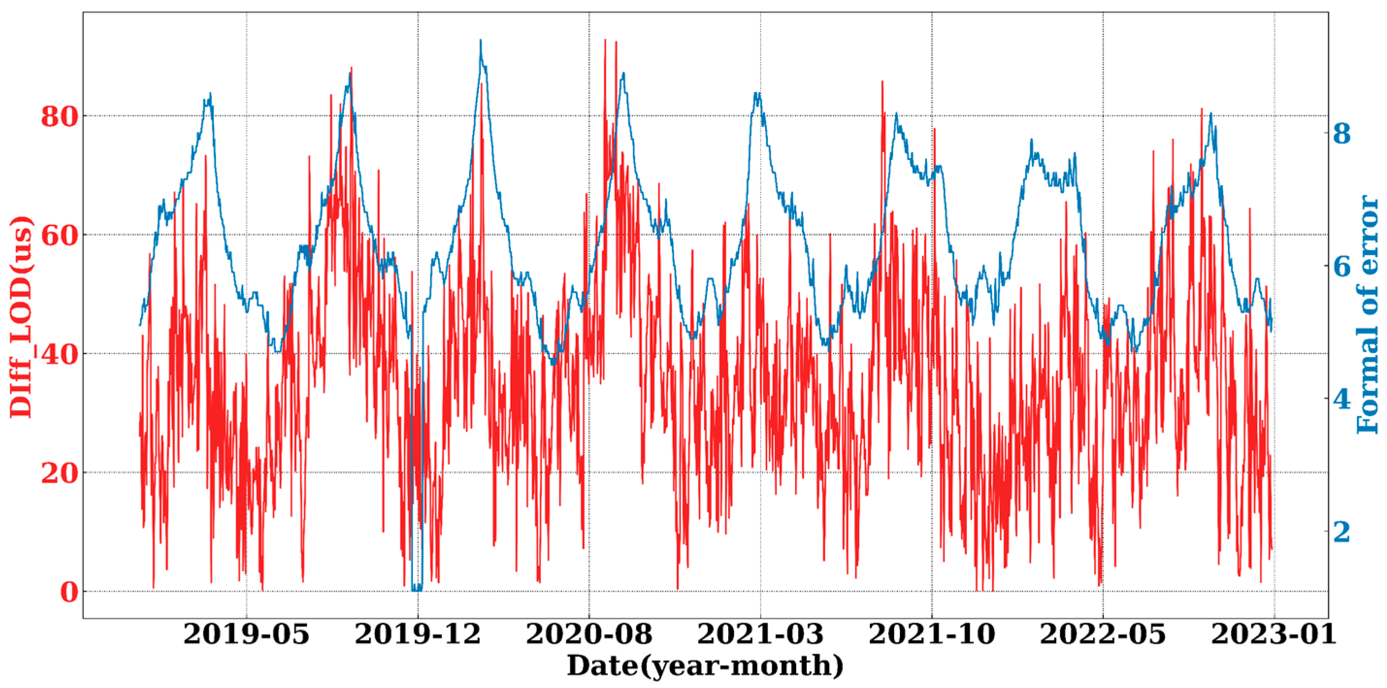
6.1. Correlation Analysis between Formal Error and Deviation

Section 4 and Section 5 indicate that combining the appropriate EAM with GNSS LODR can improve the accuracy of LOD. To further validate the rationality of using formal error as combination weights in the combination algorithm, we analyzed the correlation between the formal accuracy of GNSS LOD and its deviation from C04 LOD, as shown in Figure 12.
From Figure 12, we can clearly observe a strong correlation between the formal error and external fit accuracy of JPL LOD. Both exhibit consistent periodicity. Therefore, it is reasonable to use the formal error for composite weighting in our methodology, which indirectly validates the rationality of using the accuracy of the combination algorithm to assess the formal error of EAM.
The simulation experiments conducted with WHU, JPL, and iGMAS indicate that when the formal error of the EAM is 2–5 times that of GNSS LOD, a higher precision LOD composite product can be achieved. Specifically, when the formal error of EAM is in the range of 10–30 us, it can improve the LOD accuracy by more than 10%. The formal errors of WHU, JPL, and iGMAS are 1.16 us, 6.32 us, and 7.20 us, respectively. Based on the combination results and the formal accuracy of different LOD products, we suspect that the WHU LOD product may have a lower formal accuracy.

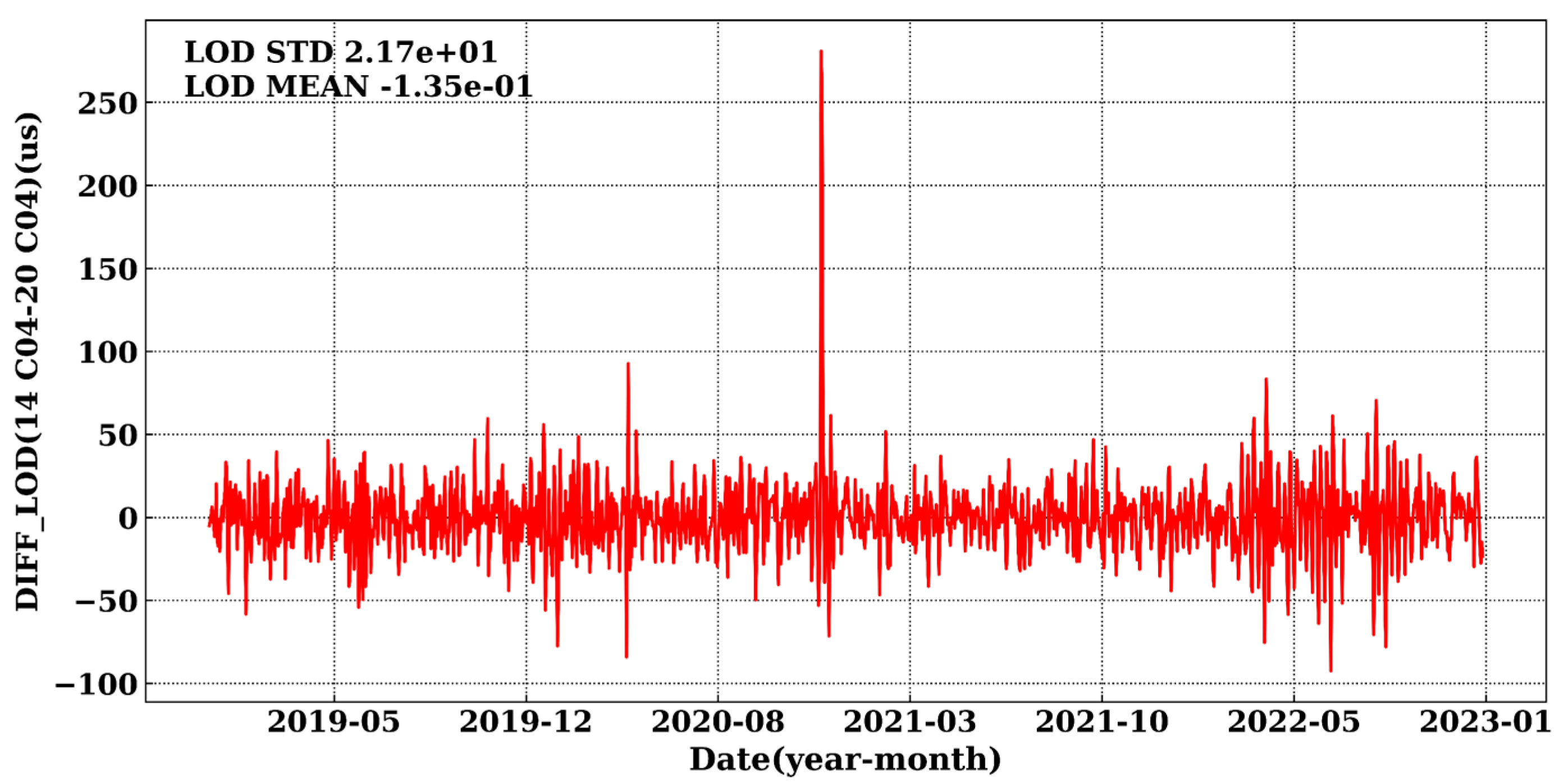
6.2. Comparison between IERS 20 C04 and IERS 14 C04

In the accuracy comparison section of this article, IERS 14 C04 was selected as the reference. This was because the IERS 20 C04 version was only released and used starting from 14 February 2023. Therefore, the IERS 14 C04 sequence was chosen for the accuracy comparison analysis in this study. Below is a brief analysis of the differences between IERS 14 C04 and IERS 20 C04.
From Figure 13, it can be observed that there seems to be a slight deviation between IERS 14 C04 and IERS 20 C04. The standard deviation of the difference in LOD values is 21.7 us. We noticed that LOD values in IERS 20 C04 and IERS 14 C04 exhibited a mismatch on 20 December 2020. The difference in LOD values was around 300 us. We suspect that this difference on 20 December 2020 may be abnormal.
Based on the analysis above, it can be concluded that even in the case of IERS C04 products, there is a possibility of encountering abnormal values, and there is a fluctuation of 20 us in LOD values between the two versions. Therefore, we recommend that IERS considers adding the EAM dataset when performing EOP combination to enhance the robustness of the data.

6.3. Prospects

Using the EAM dataset can improve the combination accuracy of LOD, but it cannot correct the systematic bias of LOD. If we want to further correct the systematic bias of LOD, we can only use the UT1 dataset for correction. For example, the final products and rapid products of IGS use the UT1 dataset for correcting the systematic bias. Considering this, we propose some follow-up plans:
(a)
Carry out EAM, LOD, and UT1 combination algorithms to improve the accuracy of LOD while further correcting the system bias of LOD, and attempt to obtain higher accuracy UT1 and EAM sequences.
(b)
Further analyze and validate the formal error of EAM. This involves conducting in-depth investigations into the sources and magnitudes of error in the EAM dataset, with the aim of improving its reliability and accuracy.
(c)
Apply the LOD obtained from the combination of EAM and LOD to EOP prediction. This can compensate for the one-day delay in EOP rapid LOD products, thus enhancing the accuracy of EOP prediction.
(d)
Conduct experiments combining polar motion (PM) and EAM to explore the impact of EAM on PM. This research aims to understand how the EAM dataset can be utilized to improve the prediction and modeling of PM.

7. Conclusions

Due to the improvement in the accuracy of atmospheric and oceanic angular momentum models based on global meteorological and oceanographic monitoring data, as well as their high correlation with LOD, this paper proposes a combination method of EAM (AAM + OAM + HAM + SLAM) and GNSS LOD data at the residual level. The combination method is validated using the LOD datasets from WHU and JPL over a 4-year time scale. The influence of EAM on the accuracy of LOD combination under different formal errors is simulated, and we attempted to determine the reasonable range of formal error for EAM based on the simulation results. The main conclusions are as follows:
(a)
After applying the EAM dataset with reasonable formal error, the LOD accuracy can be improved by 10–20%. However, this does not correct its systematic error.
(b)
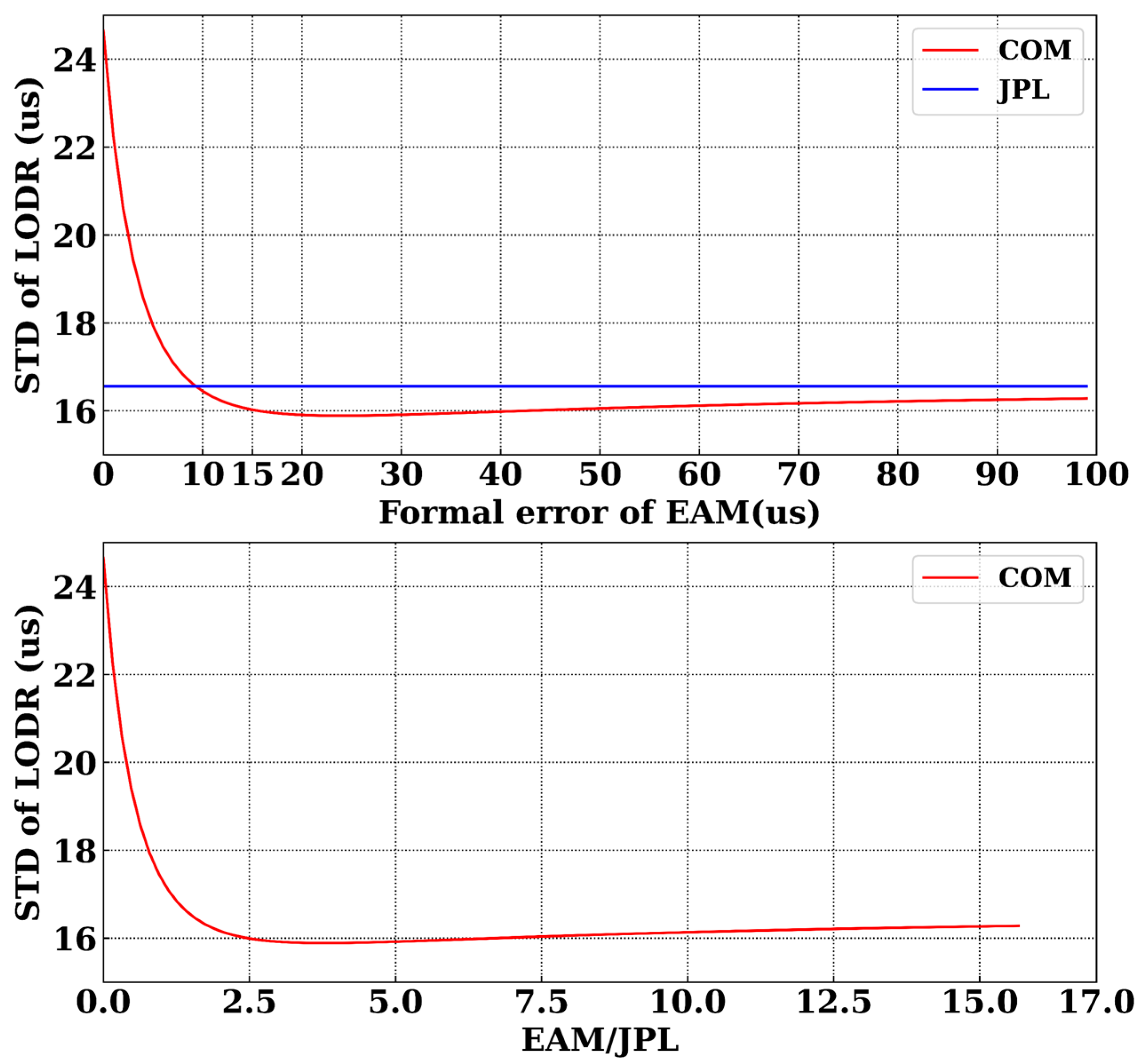
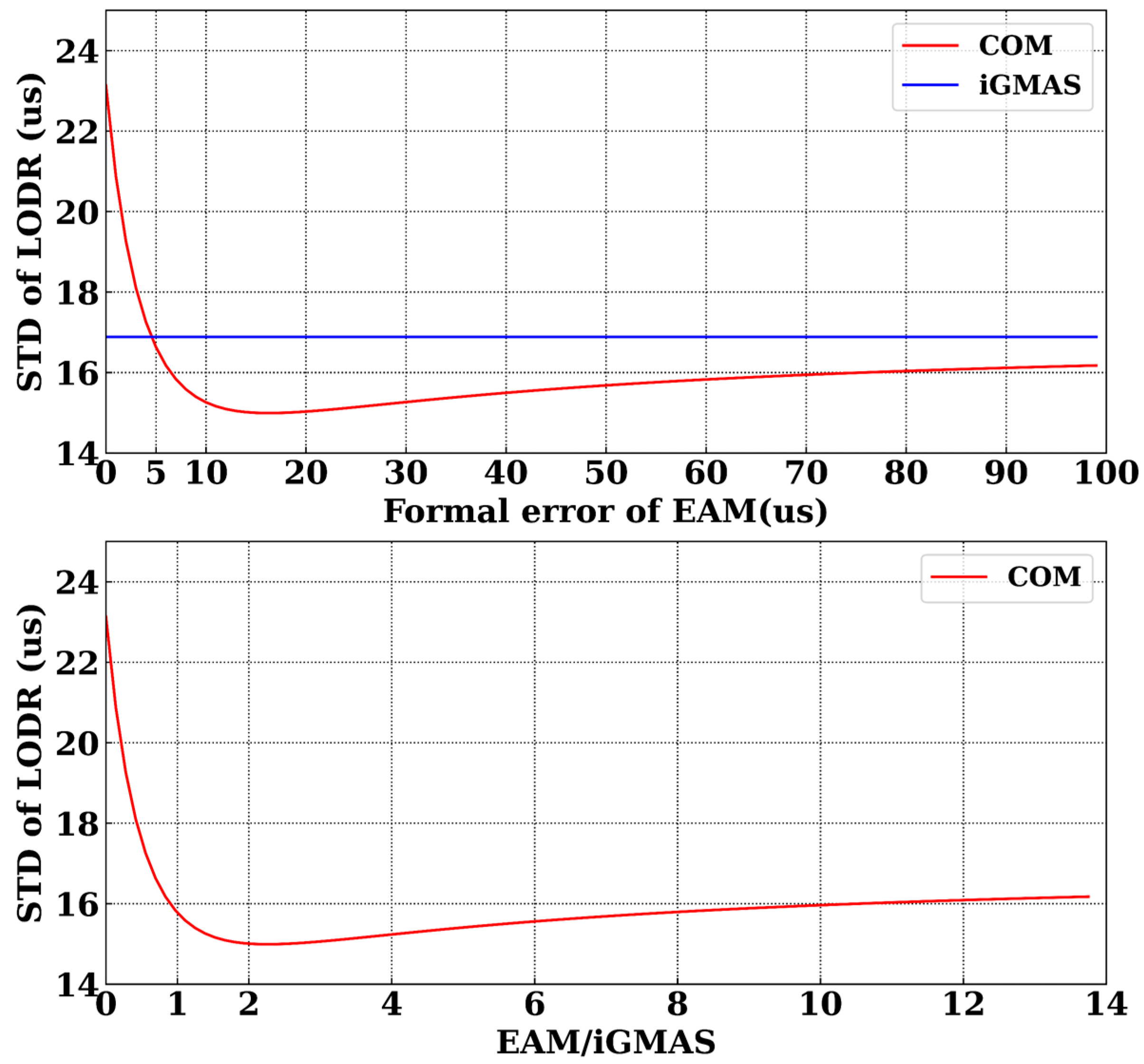
Through simulation experiments, we have determined that when the formal error of the EAM dataset is 2–5 times that of the GNSS LOD dataset, specifically within the range of 10–30 us, the combined accuracy of LOD is significantly improved.
(c)
We have analyzed the correlation between the formal error of GNSS LOD and the accuracy of external conformity. Through both simulation and actual measurement data, it has been demonstrated that using formal accuracy weighting in the combination process is a valid approach.

Author Contributions

Conception and design were performed by X.L., X.Y., R.Y., X.C. and S.Z. Material preparation, data collection, and analysis were performed by X.L. and X.Y. Implementation and validation of the combination algorithms were performed by X.L., X.Y. and R.Y. The first draft of the manuscript was written by X.L. and all authors commented on previous versions of the manuscript. All authors have read and agreed to the published version of the manuscript.

Funding

This study was funded by the General Program of the National Natural Science Foundation of China (12073034) and iGMAS project (WDS2022003).

Data Availability Statement

The IERS C04 can be downloaded at http://hpiers.obspm.fr/iers/eop/eopc04/eopc04_IAU2000.62-now (accessed on 1 December 2023), the iGMAS LOD can be downloaded at http://124.205.50.178 (accessed on 1 December 2023), and the EAM can be downloaded at http://esmdata.gfz-potsdam.de:8080 (accessed on 1 December 2023).

Acknowledgments

This article uses IERS C04 sequences, JPL LOD sequences, WHU LOD sequences, iGMAS LOD sequences, and GFZ EAM (AAM, OAM, HAM, SLAM) sequences. We would like to express our gratitude to the data provider.

Conflicts of Interest

The authors declare no conflicts of interest.

References

  1. Petti, G.; Luzum, B. IERS Conventions 2010; Verlag des Bundesamts für Kartographie und Geodäsie: Frankfurt am Main, Germany, 2010; ISBN 3-89888-989-6. [Google Scholar]
  2. Kalarus, M.; Schuh, H.; Kosek, W.; Akyilmaz, O.; Bizouard, C.; Gambis, D.; Gross, R.; Jovanovi’c, B.; Kumakshev, S.; Kutterer, H.; et al. Achievements of the Earth orientation parameters prediction comparison campaign. J. Geod. 2010, 84, 587–596. [Google Scholar] [CrossRef]
  3. Zheng, D.W.; Yu, N.H. The Earth’s Rotation and Its Relationship with Geophysical Phenomena. Prog. Geophys. 1996, 2, 81–104. [Google Scholar]
  4. Nastula, J.; Chin, T.M.; Gross, R.; Śliwińska, J.; Wińska, M. Smoothing and predicting celestial pole offsets using a Kalman filter and smoother. J. Geod. 2020, 94, 2–17. [Google Scholar] [CrossRef]
  5. Gambis, D.; Luzum, B. Earth rotation monitoring, UT1-UTC determination and prediction. Metrologia 2011, 48, 165–170. [Google Scholar] [CrossRef]
  6. Gambis, D.; Biancale, R.; Carlucci, T.; Lemoine, J.M.; Marty, J.C.; Bourda, G.; Charlot, P.; Loyer, S.; Lalanne, T.; Soudarin, L.; et al. Combination of Earth Orientation Parameters and Terrestrial Frame at the Observation Level. In International Association of Geodesy Symposia; Springer: Berlin/Heidelberg, Germany, 2009; Volume 134, pp. 3–9. [Google Scholar] [CrossRef]
  7. Byram, S.; Hackman, C. High-precision GNSS orbit, clock and EOP estimation at the United States Naval Observatory. In Proceedings of the 2012 IEEE/ION Position, Location and Navigation Symposium, Myrtle Beach, SC, USA, 23–26 April 2012. [Google Scholar] [CrossRef]
  8. Hein, G.W. Status, perspectives and trends of satellite navigation. Satell. Navig. 2020, 1, 22. [Google Scholar] [CrossRef] [PubMed]
  9. Nilsson, T.; Böhm, J.; Schuh, H. Universal time from VLBI single-baseline observations during CONT08. J. Geod. 2011, 85, 415–423. [Google Scholar] [CrossRef]
  10. Nilsson, T.; Heinkelmann, R.; Karbon, M.; Raposo-Pulido, V.; Soja, B.; Schuh, H. Earth orientation parameters estimated from VLBI during the CONT11 campaign. J. Geod. 2014, 88, 491–502. [Google Scholar] [CrossRef]
  11. Coulot, D.; Pollet, A.; Collilieux, X.; Berio, P. Global optimization of core station networks for space geodesy: Application to the referencing of the SLR EOP with respect to ITRF. J. Geod. 2010, 84, 31. [Google Scholar] [CrossRef]
  12. Pavlov, D. Role of lunar laser ranging in realization of terrestrial, lunar, and ephemeris reference frames. J. Geod. 2020, 94, 5. [Google Scholar] [CrossRef]
  13. Willis, P.; Fagard, H.; Ferrage, P.; Lemoine, F.G.; Noll, C.E.; Noomen, R.; Otten, M.; Ries, J.C.; Rothacher, M.; Soudarin, L.; et al. The international DORIS service (IDS): Toward maturity. Adv. Space Res. 2010, 45, 1408–1420. [Google Scholar] [CrossRef]
  14. Moreaux, G.; Lemoine, F.G.; Capdeville, H.; Kuzin, S.; Otten, M.; Štěpánek, P.; Willis, P.; Ferrage, P. The international DORIS service contribution to the 2014 realization of the international terrestrial reference frame. Adv. Space Res. 2016, 58, 2479–2504. [Google Scholar] [CrossRef]
  15. Bizouard, C.; Lambert, S.; Gattano, C.; Becker, O.; Richard, J.-Y. The IERS EOP 14C04 solution for Earth orientation parameters consistent with ITRF 2014. J. Geod. 2019, 93, 621–633. [Google Scholar] [CrossRef]
  16. Artz, T.; Bernhard, L.; Nothnagel, A.; Steigenberger, P.; Tesmer, S. Methodology for the combination of sub-daliy earth rotation from GPS and VLBI observations. J. Geod. 2012, 86, 221–239. [Google Scholar] [CrossRef]
  17. Barnes, R.T.H.; Hide, A.; White, A.; Wilson, C.A. Atmospheric angular momentum fluctuations. Length-of-day changes and polar motion. Proc. R. Soc. Lond. Ser. A Math. Phys. Eng. Sci. 1983, 387, 31–73. [Google Scholar] [CrossRef]
  18. Rosen, R.D.; Salstein, D.A. Variations in atmospheric angular momentum on global and regional scales and the length of day. J. Geophys. Res-Oceans 1983, 88, 5451–5470. [Google Scholar] [CrossRef]
  19. Gross, R.S.; Fukumori, I.; Menemenlis, D.; Gegout, P. Atmospheric and oceanic excitation of length-of-day variations during 1980–2000. J. Geophys. Res. Solid Earth 2004, 109, 1–15. [Google Scholar] [CrossRef]
  20. Rekier, J.; Chao, B.F.; Chen, J.L.; Dehant, V.; Rosat, S.; Zhu, P. Earth’s Rotation: Observations and Relation to Deep Interior. Surv. Geophys. 2022, 43, 149–175. [Google Scholar] [CrossRef]
  21. Dickey, J.O.; Marcus, S.L.; Steppe, J.A.; Hide, R. The Earth’s angular momentum budget on sub-seasonal time scales. Science 1992, 255, 321–324. [Google Scholar] [CrossRef] [PubMed]
  22. Freedman, A.P.; Steppe, J.A.; Dickey, J.O.; Eubanks, T.M.; Sung, L.Y. The short-term prediction of universal time and length of day using atmospheric angular momentum. J. Geophys. Res. 1994, 99, 6981–6996. [Google Scholar] [CrossRef]
  23. Johnson, T.J.; Luzum, B.J.; Ray, J.R. Improved near-term Earth rotation predictions using atmospheric angular momentum analysis and forecasts. J. Geodyn. 2005, 39, 209–221. [Google Scholar] [CrossRef]
  24. Dill, R.; Dobslaw, H. Short-term polar motion forecasts from earth system modeling data. J. Geod. 2010, 284, 529–536. [Google Scholar] [CrossRef]
  25. Dill, R.; Dobslaw, H.; Thomas, M. Improved 90-day Earth orientation predictions from angular momentum forecasts of atmosphere, ocean, and terrestrial hydrosphere. J. Geod. 2019, 93, 287–295. [Google Scholar] [CrossRef]
  26. Li, X.; Wu, Y.; Yao, D.; Liu, J.; Nan, K.; Ma, L.; Cheng, X.; Yang, X.; Zhang, S. Research on UT1-UTC and LOD Prediction Algorithm Based on Denoised EAM Dataset. Remote Sens. 2023, 15, 4654. [Google Scholar] [CrossRef]
  27. Jungclaus, J.H.; Fischer, N.; Haak, H.; Lohmann, K.; Marotzke, J.; Matei, D.; Mikolajewicz, U.; Notz, D.; VonStorch, J.S. Characteristics of the ocean simulations in the Max Planck Institute Ocean Model (MPIOM) the ocean component of the MPI-Earth system model. J. Adv. Model. EarthSyst. 2013, 5, 422–446. [Google Scholar] [CrossRef]
  28. Dill, R. Hydrological Model LSDM for Operational Earth Rotation and Gravity Field Variations; Scientific Technical Report STR; 08/09; GFZ: Potsdam, Germany, 2008; p. 35. [Google Scholar]
  29. Dobslaw, H.; Dill, R.; Grötzsch, A.; Brzezinski, A.; Thomas, M. Seasonal polar motion excitation from numerical models of atmosphere, ocean, and continental hydrosphere. J. Geophys. Res. 2010, 115, 406. [Google Scholar] [CrossRef]
  30. Tamisiea, M.E.; Hill, E.M.; Ponte, R.M.; Davis, J.L.; Velicogna, I.; Vinogradova, N.T. Impact of self-attraction and loading on the annual cycle in sea level. J. Geophys. Res. 2010, 115, 1–15. [Google Scholar] [CrossRef]
  31. Hagemann, S.; Dumenil, L. A parametrization of the waterflow for the global scale. Clim. Dynam. 1998, 14, 17–31. [Google Scholar] [CrossRef]
  32. Ding, H.; Chao, F. Application of Stabilized AR-z Spectrum in Harmonic Analysis for Geophysics. J. Geophys. Res. Solid Earth 2018, 123, 8249–8259. [Google Scholar] [CrossRef]
  33. Chao, B.F.; Chung, W.Y.; Shih, Z.; Hsieh, Y. Earth’s rotation variations: A wavelet analysis. Terra Nova 2014, 26, 260–264. [Google Scholar] [CrossRef]
  34. Ray, R.D.; Erofeeva, S.Y. Long-period tidal variations in the length of day. J. Geophys. Res. 2014, 119, 1498–1509. [Google Scholar] [CrossRef]
  35. Hung, L.S.; Anderson, B.D.O. Design of Kalman filters using signal-model output statistics. Proc. Inst. Electr. Eng. UK 1973, 120, 312–318. [Google Scholar]
  36. Welch, G.; Bishop, G. An Introduction to the Kalman Filter; ACM, Inc.: Chicago, IL, USA, 2001; pp. 1–24. [Google Scholar]
  37. Nahi, N.E. Estimation Theory and Applications; John Wiley and Sons: New York, NY, USA, 1969. [Google Scholar]
  38. Bierman, G.J. Factorization Methods for Discrete Sequential Estimation; Academic Press: New York, NY, USA, 1977. [Google Scholar]
  39. Rosen, R.D.; Salstein, D.A.; Miller, A.J.; Arpe, K. Accuracy of atmospheric angular momentum estimates from operational analyses. Mon. Weather Rev. 1987, 115, 1627–1639. [Google Scholar] [CrossRef]
  40. Gross, R.S.; Eubanks, T.M. Estimating the “noise” component of various atmospheric angular momentum time series (abstract). Eos Trans. AGU 1988, 69, 1153. [Google Scholar]
  41. Bell, M.J.; Hide, R.; Sakellarides, G. Atmospheric angular momentum forecasts as novel tests of global numerical weather prediction models. Philos. Trans. R. Soc. Lond. Set. A 1991, 334, 55–92. [Google Scholar]
  42. Gross, R.S.; Steppe, J.A.; Dickey, J.O. The running RMS difference between length-of-day and various measures of atmospheric angular momentum. In Proceedings of the AGU Chapman Conference on Geodetic VLBI: Monitoring Global Change, Washington, DC, USA, 22–26 April 1991; NOAA Tech. Rgp. NOS 137 NGS 49. Natl. Ocean Serv., NOAA: Silver Spring, MD, USA, 1991; pp. 238–258. [Google Scholar]
Figure 1. The red and black lines in the top panel represent the C04 LODR and the LODR derived from EAM, respectively. The bottom panel displays the difference between the LODR derived from EAM and the C04 LODR, represented by the black line.
Remotesensing 16 00722 g001
Figure 2. Correlation coefficient between EAM LODR and C04 LODR. It can be observed that the EAM LODR and the C04 LODR exhibit a strong positive correlation, with a correlation coefficient of 0.916.
Remotesensing 16 00722 g002
Figure 3. The red, green, and light blue lines in the top panel represent the LODR data from C04, WHU, and JPL, respectively. In the bottom panel, the green and light blue lines represent the difference between WHU and C04 LODR, and JPL and C04 LODR, respectively. To facilitate distinction, a bias of −50 us was added to the JPL and C04 LODR difference.
Remotesensing 16 00722 g003
Figure 4. In the top panel, the red, black, and green lines represent the first-order difference in LODR data for C04 and WHU, as well as the difference between WHU LODR and C04 LODR. To facilitate distinction, a deviation of −100 us is added to the first-order difference in WHU LODR data and the difference between WHU LODR and C04 LODR. The black and green lines in the bottom panel correspond to the first-order difference in WHU LODR after removing outlier points, and the difference between WHU and C04 LODR after outlier removal, respectively.
Remotesensing 16 00722 g004
Figure 5. In the top panel, the red, green, light blue, and black lines represent the LODR sequences for C04, WHU, JPL, and EAM, respectively. In the middle panel, the red, green, light blue, and black lines represent the least squares fitting of LODR for C04, WHU, JPL, and EAM, respectively. In the bottom panel, the red, green, light blue, and black lines represent the residual terms of the least squares fits for C04, WHU, JPL, and EAM LODR data, respectively.
Remotesensing 16 00722 g005
Figure 6. The red and black lines in the top panel represent the residual of EAM LODR least squares fitting and the residual of EAM LODR least squares fitting after Kalman filtering, respectively. The red and black lines in the bottom panel represent the difference between the EAM LODR least squares fitting residuals and the C04 LODR least squares fitting residuals, as well as the difference between the EAM LODR least squares fitting residuals after Kalman filtering and the C04 LODR least squares fitting residuals.
Remotesensing 16 00722 g006
Figure 7. The blue line in the top panel represents the accuracy of WHU LODR, which is the standard deviation of the difference between WHU LODR and C04 LODR. The red line represents the accuracy of the combined WHU LODR and EAM LODR with a different formal error (denoted as COM). The bottom panel shows the variation in LODR combination accuracy between EAM and WHU LODR with respect to the ratio of formal error in EAM and WHU LODR.
Remotesensing 16 00722 g007
Figure 8. The description of Figure 8 is similar to Figure 7, with the only difference being the replacement of WHU LODR with JPL LODR.
Remotesensing 16 00722 g008
Figure 9. The description of Figure 9 is similar to Figure 7, with the only difference being the replacement of WHU LODR with iGMAS LODR.
Remotesensing 16 00722 g009
Figure 10. The green line in the top panel represents the difference between the WHU LOD (after removing outliers) and C04 LOD, while the red line represents the difference between the combined LOD (WHU LOD and EAM) and C04 LOD. To enhance clarity in the comparison results, a 50 us offset is added to the difference between WHU and C04 LOD in the graph. The bottom panel is a histogram that shows the distribution of the differences displayed in the top panel. The x-axis represents the difference values in microseconds, and the y-axis represents probability. To improve visual representation, a curve fitting is applied to the histogram. The distributions of the two types of differences all follow normal distribution. The red and green lines are normal distribution curves with the fitted mean and standard deviation listed in Table 2.
Remotesensing 16 00722 g010
Figure 11. The description of Figure 11 is similar to Figure 10, with the only difference being the replacement of WHU LODR with JPL LODR.
Remotesensing 16 00722 g011
Figure 12. The formal accuracy of JPL LOD and its deviation from C04 LOD. The blue line represents the uncertainty, i.e., formal error, of JPL LOD. The red line represents the difference between JPL LOD and C04 LOD, i.e., external fit accuracy.
Remotesensing 16 00722 g012
Figure 13. Difference in LOD between 14 C04 and 20 C04 from 2019 to 2023.
Remotesensing 16 00722 g013
Table 1. Effective Angular Momentum of Earth.
AngularTime ResolutionUpdate FrequencyProportion
AAM3 h24 h97.6%
OAM3 h24 h0.8%
HAM24 h24 h0.5%
SLAM24 h24 h1.1%
Table 2. Statistics of combined WHU and EAM.
ProductsSTD
(us)
MEAN
(us)
MEDIAN (us)MAX
(us)
MIN
(us)
WHU13.51−20.28−19.8621.29−63.12
COM10.57−20.27−19.8912.56−58.97
Table 3. Statistics of combined JPL and EAM.
ProductsSTD
(us)
MEAN
(us)
MEDIAN (us)MAX
(us)
MIN
(us)
JPL17.75−34.09−33.9428.32−92.75
COM15.42−34.06−33.6810.27−83.98
Disclaimer/Publisher’s Note: The statements, opinions and data contained in all publications are solely those of the individual author(s) and contributor(s) and not of MDPI and/or the editor(s). MDPI and/or the editor(s) disclaim responsibility for any injury to people or property resulting from any ideas, methods, instructions or products referred to in the content.

