A Transfer Learning-Enhanced Generative Adversarial Network for Downscaling Sea Surface Height through Heterogeneous Data Fusion

Abstract

In recent decades, satellites have played a pivotal role in observing ocean dynamics, providing diverse datasets with varying spatial resolutions. Notably, within these datasets, sea surface height (SSH) data typically exhibit low resolution, while sea surface temperature (SST) data have significantly higher resolution. This study introduces a Transfer Learning-enhanced Generative Adversarial Network (TLGAN) for reconstructing high-resolution SSH fields through the fusion of heterogeneous SST data. In contrast to alternative deep learning approaches that involve directly stacking SSH and SST data as input channels in neural networks, our methodology utilizes bifurcated blocks comprising Residual Dense Module and Residual Feature Distillation Module to extract features from SSH and SST data, respectively. A pixelshuffle module-based upscaling block is then concatenated to map these features into a common latent space. Employing a hybrid strategy involving adversarial training and transfer learning, we overcome the limitation that SST and SSH data should share the same time dimension and achieve significant resolution enhancement in SSH reconstruction. Experimental results demonstrate that, when compared to interpolation method, TLGAN effectively reduces reconstruction errors and fusing SST data could significantly enhance in generating more realistic and physically plausible results.

1. Introduction

For decades, satellites equipped with various sensors have made observations of ocean dynamics and provided a large number of geophysical data fields at different spatial and temporal resolutions. Currently, global SSH observations are primarily achieved by spaceborne radar altimeters, which retrieve the two-dimensional SSH field (∼25 km) from altimetry observations [1,2]. In addition to satellite altimetry observations, satellites also routinely observe other ocean dynamic parameters, including SST, which can be observed at relatively higher resolution [3]. A large number of studies have revealed that SSH and SST have a close dynamic relationship [4,5,6,7,8]. In recent years, the notable advancements in deep learning within the field of computer vision have led to the emergence of numerous models designed to exploit the dynamic relationships between SSH and SST. These models seek to incorporate SST observations in SSH reconstruction, addressing challenges such as filling missing data [9] or performing data downscaling [10,11]. The former corresponds to a deep learning-based image inpainting problem applied to oceanography, while the latter falls within the domain of the deep learning-based image super-resolution (DLSR) problem. This study specifically focuses on the second area, centering on the downscaling of the SSH field within the super-resolution (SR) architecture.

Recently, Dong et al. [12] pioneered the application of deep convolutional neural network to address the image super-resolution problem and introduced a model named Super-Resolution Convolutional Neural Network (SRCNN). Subsequently, numerous researchers have actively explored enhancements to the SRCNN architecture to achieve improved performance [13]. This exploration has naturally extended to investigating the application of these techniques to scientific data downscaling [14,15]. In 2023, Thiria et al. [10] proposed a deep learning technique, REsolution by Stages of Altimetry and Currents (RESAC), based on the SRCNN architecture. RESAC aims to reconstruct high-resolution SSH fields and flow fields with the asistance of high-resolution SST data. Following this, Archambault et al. [11] modified the RESAC network and introduced a subpixel convolutional residual network, named RESACsub. Most CNN-based super-resolution methods typically seek to maximize Peak Signal-to-Noise Ratio (PSNR) by minimizing the mean square error (MSE) pixel difference between the reconstructed image and the high-resolution image [12,13,16]. However, higher PSNR does not always result in perceptually superior images. Addressing this issue, Ledig et al. [17] introduced the Super-Resolution Generative Adversarial Network (SRGAN), a model based on adversarial training. SRGAN incorporates GAN-based training and perceptual loss functions to generate super-resolution images with enhanced visualization effects, diverging from a sole focus on strategies to maximize PSNR. In this study, we employ a GAN-based super-resolution method to augment the spatial resolution of the SSH field. To the best of the authors’ knowledge, this method is applied to this problem for the first time.

In RESAC and RESACsub, all selected variables (SSH and SST) are directly stacked to create a three-dimensional tensor as the input of the neural network models. This practice of directly stacking variables as distinct input channels aligns with methodologies employed in other downscaling studies [18]. While this approach is straightforward, the amalgamation of these heterogeneous variables, which differ significantly in characteristics, can pose challenges during the training process. Consequently, in this study, we opt to extract features from each variable before their concatenation. The existing models are trained utilizing SSH and SST data characterized by different spatial resolutions yet necessitating an identical time dimension. However, this study considers a more general scenario. In comparison to SST data, SSH data not only exhibits lower spatial resolution but also involves a smaller data volume in the time dimension. Additionally, considering the distinctive feature characteristics of SSH and SST fields, we introduce the Residual Dense Module (RDM) and the Residual Feature Distillation Module (RFDM) to extract features from SSH and SST, respectively. The RDM, with a more intricate structure, is employed to extract features from SSH, characterized by a smaller data volume. Conversely, the RFDM, designed with a simpler structure, facilitates easier training for feature extraction from SST, which involves a larger data volume. Subsequently, we adopt a multi-stage transfer learning strategy that encompasses the transfer of parameter knowledge [19]. This strategy enables the model to address the challenge of recovering SSH from disparate feature spaces or different data distributions.

2. TLGAN Model

2.1. Network Architecture

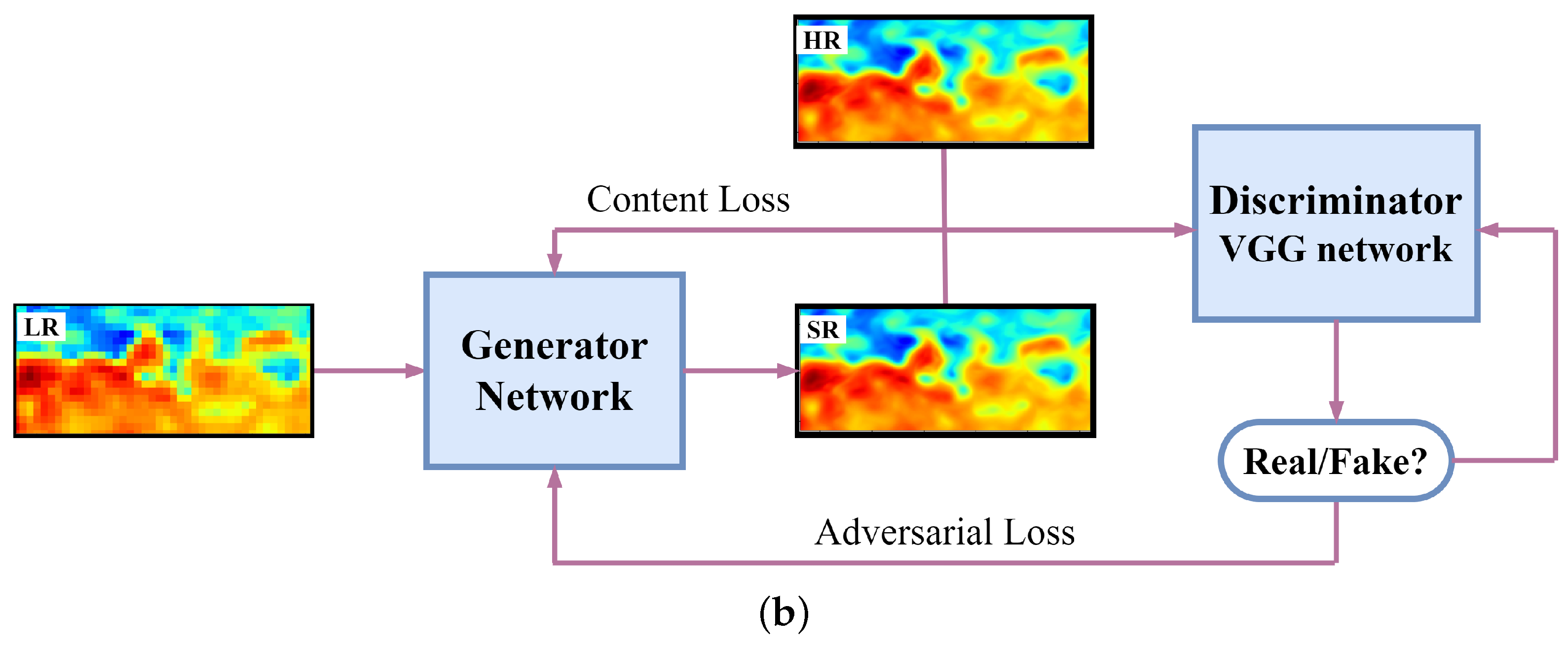
The TLGAN comprises a Generator $G\left(\mathrm{\Theta }\right)$ and a Discriminator $D\left(\mathrm{\Phi }\right)$, illustrated in Figure 1b. The Discriminator $D\left(\mathrm{\Phi }\right)$ employs the robust and established VGG model [20]. The VGG model, a convolutional neural network (CNN) architecture devised by the Visual Geometry Group at the University of Oxford, was initially proposed for image classification tasks and has since found widespread application in various computer vision domains [21]. Renowned for its simplicity and efficacy, the VGG model comprises multiple convolutional layers succeeded by max-pooling layers, culminating in fully connected layers for classification purposes. Its distinctive characteristic lies in its deep architecture featuring small (3 × 3) convolutional filters stacked sequentially, enabling it to discern intricate features within images. In the context of this study, the VGG model serves as the discriminator, tasked with assessing the realism or quality of the reconstructed SSH field produced by the TLGAN model. This evaluation is accomplished by comparing the features extracted from the reconstructed SSH data against those extracted from the original SSH data. Consequently, the discriminator (VGG model) furnishes feedback to the TLGAN model, thereby facilitating enhancements to the quality of its generated outputs. On the other hand, $G\left(\mathrm{\Theta }\right)$ encompasses three key blocks: the residual dense block $G_1\left({\mathrm{\Theta }}_1\right)$, the residual feature distillation block $G_2\left({\mathrm{\Theta }}_2\right)$, and the upscaling block $G_3\left({\mathrm{\Theta }}_3\right)$, where ${\mathrm{\Theta }}_1$, ${\mathrm{\Theta }}_2$, and ${\mathrm{\Theta }}_3$ represent the parameters for the respective blocks (see Figure 1a). $G_1\left({\mathrm{\Theta }}_1\right)$ serves as an SSH feature extractor, commencing with a single convolutional layer for shallow feature extraction followed by multiple Residual Dense Modules (RDMs) [22]. Each RDM comprises a dense network with local fusion, facilitating direct connections between the preceding RDM state and all layers of the current RDM. Local fusion enhances the learning of features from the preceding and current states effectively, while global feature fusion, implemented after the RDMs, enables joint and adaptive learning of global hierarchical features. This architecture mitigates the vanishing gradient problem through dense and residual connections, reinfusing previous information during training. $G_2\left({\mathrm{\Theta }}_2\right)$ is primarily composed of Residual Feature Distillation Modules (RFDM) [23]. The RFDM concept draws inspiration from the Information Distillation Network (IDN), a framework that combines present information with local data through an information distillation network. In the RFDM, convolutional layers at various levels extract features at different levels. Operations such as deconvolution allow shallow neural networks to focus on parts akin to image contours, while deeper networks concentrate on information such as texture details. $G_3\left({\mathrm{\Theta }}_3\right)$ utilizes the efficient pixelshuffle convolutional module to achieve an 8× downscaling factor [24]. This architectural design integrates multisource feature fusion and scale conversion, contributing to the overall capabilities of TLGAN in SSH field reconstruction.

2.2. Training Strategy

The proposed model is trained using a combination of adversarial training and transfer learning. The generator network reconstructs the high-resolution (HR) images by mapping input low-resolution (LR) images to the space of the associated super-resolution (SR) images (as shown in Figure 1b). The discriminator network classifies the SR images as real (from the training set) or fake (generated by the generator network). The two networks undergo iterative training, with the generator producing more realistic fields over time and the discriminator becoming more adept at distinguishing between real and fake data. The parameters of TLGAN are updated in three stages:

Stage I: The parameters of the entire TLGAN undergo training using adversarial training, expressed as a min–max optimization problem:

$$\underset{\mathrm{\Theta }}{min}\underset{\mathrm{\Phi }}{max}\mathbb{E}[logD\left(I^{HR}\right)]+\mathbb{E}[log(1-D\left(G\left(I^{LR}\right)\right))]$$

(1)

where $G\left(I^{LR}\right)$ denotes the generated SR image and $D\left(G\left(I^{LR}\right)\right)$ denotes the probability of generating the original HR image $I_{HR}$.

The loss function for the generator G is composed of content and advertisal terms. The content loss employs the MSE loss as:

$${\mathcal{L}}_{content}(I^{LR},I^{HR})=\left|\right|I^{HR}-G\left(I^{LR}\right){\left|\right|}_2^2$$

(2)

The adversarial loss assesses the generator’s ability to deceive the discriminator, defined as:

$${\mathcal{L}}_{adv}(I^{LR},I^{HR})=-log(1-D\left(G\left(I^{LR}\right)\right)$$

(3)

The overall loss function for the proposed model is presented as:

$${\mathcal{L}}_G(I^{LR},I^{HR})={\mathcal{L}}_{content}(I^{LR},I^{HR})+\alpha {\mathcal{L}}_{adv}(I^{LR},I^{HR})$$

(4)

where $\alpha$ is learning rate. After network update convergence, only the parameters of the residual dense block $G_1\left({\mathrm{\Theta }}_1\right)$ are retained, and the data distribution characteristics of the SSH data are saved. These parameters are not updated in subsequent training.

Stage II: The goal at this stage is to extract features or feature spaces from SST images. The training dataset at this stage comprises SST images. The $G_1\left({\mathrm{\Theta }}_1\right)$ from Stage I is not updated, and other model parameters are updated by training as follows:

$$\begin{array}{cc}\underset{\mathrm{\Theta }}{min}\underset{\mathrm{\Phi }}{max}\hfill & \mathbb{E}[logD\left(I^{HR}\right)]\hfill \end{array}$$

(5)

$$\begin{array}{cc}\hfill & +\mathbb{E}[log(1-D\left(G\left(I^{LR}\right)\right)|G_1\left({\mathrm{\Theta }}_1\right)]\hfill \end{array}$$

(6)

After this stage, the feature space $G_2\left({\mathrm{\Theta }}_2\right)$ of the SST is obtained when the network has converged.

Stage III: In this stage, the aim is to improve the overall perceptual quality of SR for small SSH samples. A small sample of SSH image datasets is selected as the training dataset, and only the parameters of Stage III are retrained. The parameters of $G_1\left({\mathrm{\Theta }}_1\right)$ and $G_2\left({\mathrm{\Theta }}_2\right)$ are not updated:

$$\begin{array}{cc}\hfill \underset{\mathrm{\Theta }}{min}\underset{\mathrm{\Phi }}{max}& \mathbb{E}[logD\left(I^{HR}\right)]\hfill \end{array}$$

(7)

$$\begin{array}{cc}\hfill & +\mathbb{E}[log(1-D\left(G\left(I^{LR}\right)\right)|G_1\left({\mathrm{\Theta }}_1\right),G_2\left({\mathrm{\Theta }}_2\right))]\hfill \end{array}$$

(8)

Finally, the feature space parameters $G\left(\mathrm{\Theta }\right)$ of the entire TLGAN are obtained through this multi-stage training strategy. The parameters are represented as $\mathrm{\Theta }=({\mathrm{\Theta }}_1,{\mathrm{\Theta }}_2,{\mathrm{\Theta }}_3)$.

3. Experiments

3.1. Datasets

In this study, our primary focus is on spatial downscaling, under the assumption that SSH and SST measurements are gridded daily observations of varying resolutions. To address the scarcity of high-resolution ocean parameter observations, we utilized the Global Ocean Reanalysis and Simulations version 1 (hereafter GLORYS12V1) reanalysis datasets provided by Copernicus Marine Environment Monitoring Service [25]. Global observations, including along-track satellite altimetry and satellite sea surface temperature, are jointly assimilated in the GLORYS12V1 reanalysis product by means of a reduced-order Kalman filter. GLORYS12V1 provides a global daily mean SSH and SST data on a standard regular grid at $1/{12}^{\circ }$ (approximately 8 km) from 1993 onward. We select three temporal subsets, inclduing SSH data covering January, May, and September of 2018; SST data covering January to December of 2018; and SSH data convering March, July, and November of 2018, for the three tranfer training stages, respectively. A temporal subset of SSH data covering August 2018 is constructed for evaluation. SSH data covering Feberatury, June, and October 2020 are extracted for testing. Our study specifically targets a segment of the Kuroshio Extension region (29–41°N, 142–170°E), where ocean currents and associated mesoscale dynamical features play a crucial role [26,27]. The goal of our study is to reconstruct high-resolution images from these coarsened data using the proposed model. We employ a downscaling factor of $\times 8$ to assess the performance of our model. The original high-resolution images measure $336\times 152$ pixels each. Subsequently, these high-resolution images are upscaled eight times in both dimensions, resulting in the loss of fine-scale features present in the high-resolution data. Consequently, the low-resolution images are $42\times 19$ pixels.

3.2. Evaluation Metrics

We employ four evaluation metrics, including mean square error (MSE), mean absolute error (MAE), peak signal-to-noise ratio (PSNR), and structural similarity index (SSIM), to assess the performance of the model [28]. These metrics gauge the dissimilarity in pixels and the structural similarity between the two images.

The MSE and MAE are used for maintaining consistency between the HR image and SR images and can be mathematically as follows:

$$\mathit{MSE}({\mathit{I}}^{\mathit{HR}},{\mathit{I}}^{\mathit{SR}})=\frac{\mathit{1}}{\mathit{N}}\sum _{\mathit{i}=\mathit{1}}^{\mathit{N}}{({\mathit{I}}_{\mathit{i}}^{\mathit{HR}}-{\mathit{I}}_{\mathit{i}}^{\mathit{SR}})}^{\mathit{2}}$$

(9)

$$\mathit{MAE}({\mathit{I}}^{\mathit{HR}},{\mathit{I}}^{\mathit{SR}})=\frac{\mathit{1}}{\mathit{N}}\sum _{\mathit{i}=\mathit{1}}^{\mathit{N}}\left|{\mathit{I}}_{\mathit{i}}^{\mathit{HR}}-{\mathit{I}}_{\mathit{i}}^{\mathit{SR}}\right|$$

(10)

where N denote the total number of pixels in each image.

The PSNR measures the overall image similarity and focuses on assessing the degree of distortion in image colors and smooth areas and is the most widely and commonly used objective metric for evaluating image quality. The formula for PSNR is expressed as follows:

$$\mathit{PSNR}=\mathit{10}{log}_{\mathit{10}}\left(\frac{{\mathit{255}}^{\mathit{2}}}{\mathit{MSE}({\mathit{I}}^{\mathit{HR}},{\mathit{I}}^{\mathit{SR}})}\right)$$

(11)

SSIM can better reflect the subjective perception of human eyes, and the SSIM value is equal to 1 when the content and structure of the two images are identical. SSIM is calculated as follows:

$$\mathit{SSIM}({\mathit{I}}^{\mathit{HR}},{\mathit{I}}^{\mathit{SR}})=\frac{(\mathit{2}{\mu }_{\mathit{HR}}{\mu }_{\mathit{SR}}+{\mathit{C}}_{\mathit{1}})(\mathit{2}{\sigma }_{\mathit{HR},\mathit{SR}}+{\mathit{C}}_{\mathit{2}})}{({\mu }_{\mathit{HR}}^{\mathit{2}}+{\mu }_{\mathit{SR}}^{\mathit{2}}+{\mathit{C}}_{\mathit{1}})({\sigma }_{\mathit{HR}}^{\mathit{2}}+{\sigma }_{\mathit{SR}}^{\mathit{2}}+{\mathit{C}}_{\mathit{2}})}$$

(12)

where ${\mu }_{HR}$ and ${\mu }_{SR}$ are the average pixel intensities, ${\sigma }_{HR}$ and ${\sigma }_{SR}$ are the standard deviations, ${\sigma }_{HR,SR}$ is the covariance, and $C_1$ and $C_2$ are constants to prevent instability.

3.3. Model Implementation

We implemented our models based on the basicSR [29]. The basicSR is an open-source PyTorch framework designed for image super resolution tasks. This toolbox provides researchers with well-developed build-in functions to build and test their proposed models in an easier way. The network is optimized using the Adam optimizer with a learning rate of $1\times {10}^{-4}$ and a batch size of 32. The network is trained on an NVIDIA RTX A4000 GPU card (Santa Clara, CA, USA).

4. Results

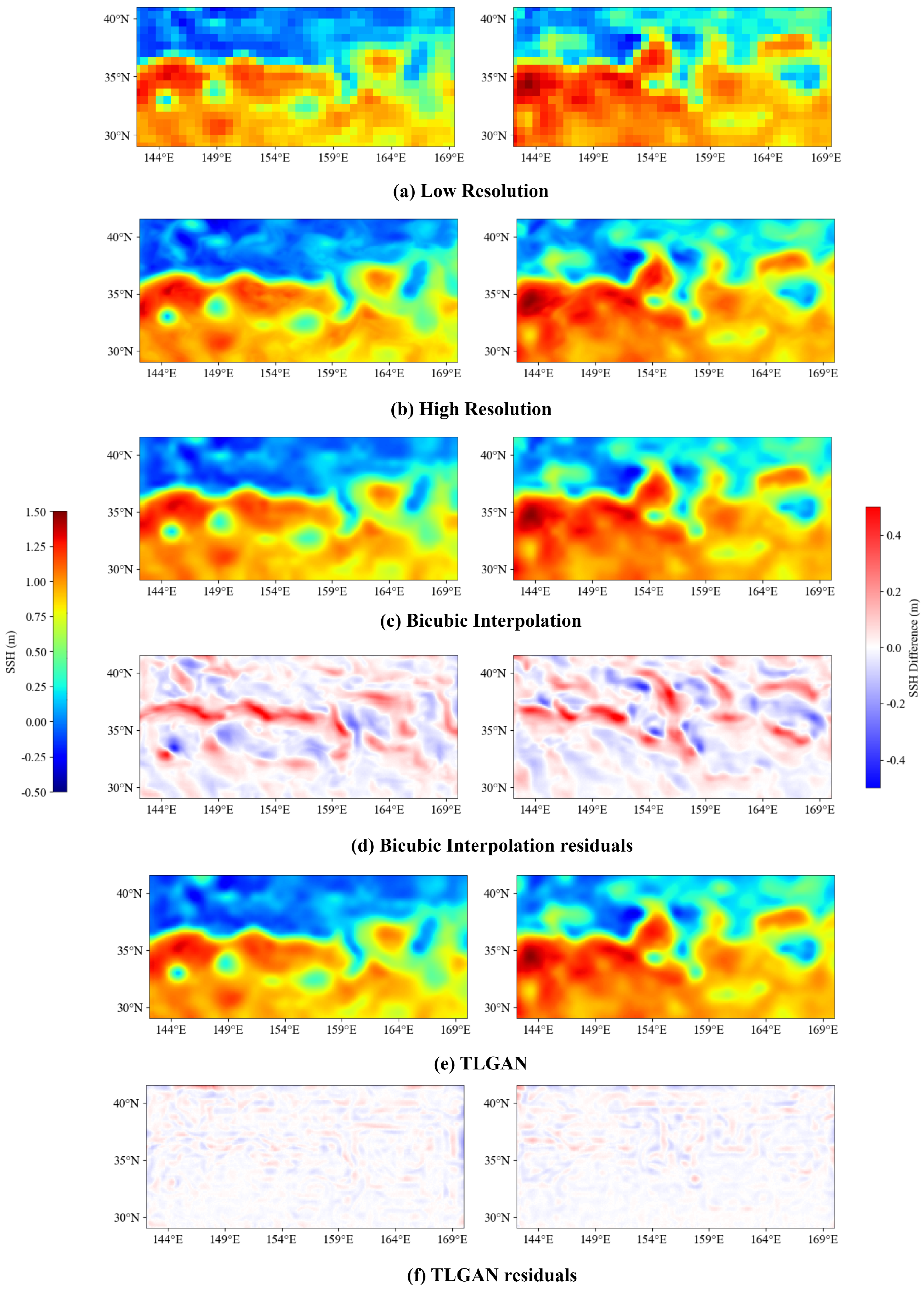
The visual representations of super-resolution (SR) image reconstruction utilizing both bicubic interpolation and the TLGAN model are presented in Figure 2. By examining solely the original high-resolution (HR) image (Figure 2b) and the reconstructed SSH fields (Figure 2c,e), discernible distinctions between TLGAN and bicubic interpolation become apparent; the latter may appear smoothed compared to the original, while the TLGAN output tends to closely resemble the original field. Bicubic interpolation, as depicted in the reconstruction, struggles to capture finer details in the HR image, a phenomenon more pronounced in Figure 2d,f, where the residuals of bicubic interpolation and TLGAN reconstruction are shown, respectively. The error reduction induced by TLGAN is evident. Notably, the most pronounced residuals for bicubic interpolation are observed in regions characterized by strong gradients. Bicubic interpolation encounters challenges in dealing with strong gradients and fails to capture subtle features, reflecting a limitation inherent in traditional interpolation methods such as bilinear or bicubic approaches. While these methods do not rely on training data, they often result in oversmoothing images, particularly missing small-scale textures and sharp edges.

To quantitatively evaluate the reconstruction performance, we computed the MSE, MAE, PSNR, and SSIM.

Table 1. Evaluation metrics for the reconstruction results. The subscripts m12 and m6 indicate that the applied SST data are 12 months and 6 months, respectively.

Model	MSE	MAE	PSNR	SSIM
Bicubic Interpolation	0.069	0.010	25.550	0.889
TLGAN(SSH+${\mathrm{SST}}_{\mathrm{m}12}$)	0.016	0.001	39.580	0.977
TLGAN(SSH+${\mathrm{SST}}_{\mathrm{m}6}$)	0.020	0.001	37.450	0.974
TLGAN(SSH only)	0.047	0.006	29.990	0.937

presents the average values of these metrics across all test data. Overall, TLGAN models exhibit significant improvement over the bicubic reconstruction results, demonstrating a decrease in MSE (from 0.0688 to 0.0164) and MAE (from 0.0104 to 0.0006). Moreover, both PSNR and SSIM show an increase. For comparative analysis, we investigated the impact of reducing the input SST data. When the SST data were halved (over a period of 6 months) or completely omitted, the reconstruction effect diminished, as indicated by an increase in MSE and a decrease in PSNR. Nevertheless, when contrasted with the bicubic interpolation method, an overall improvement was still evident. This underscores the positive contribution of incorporating SST information to the high-resolution reconstruction of SSH fields.

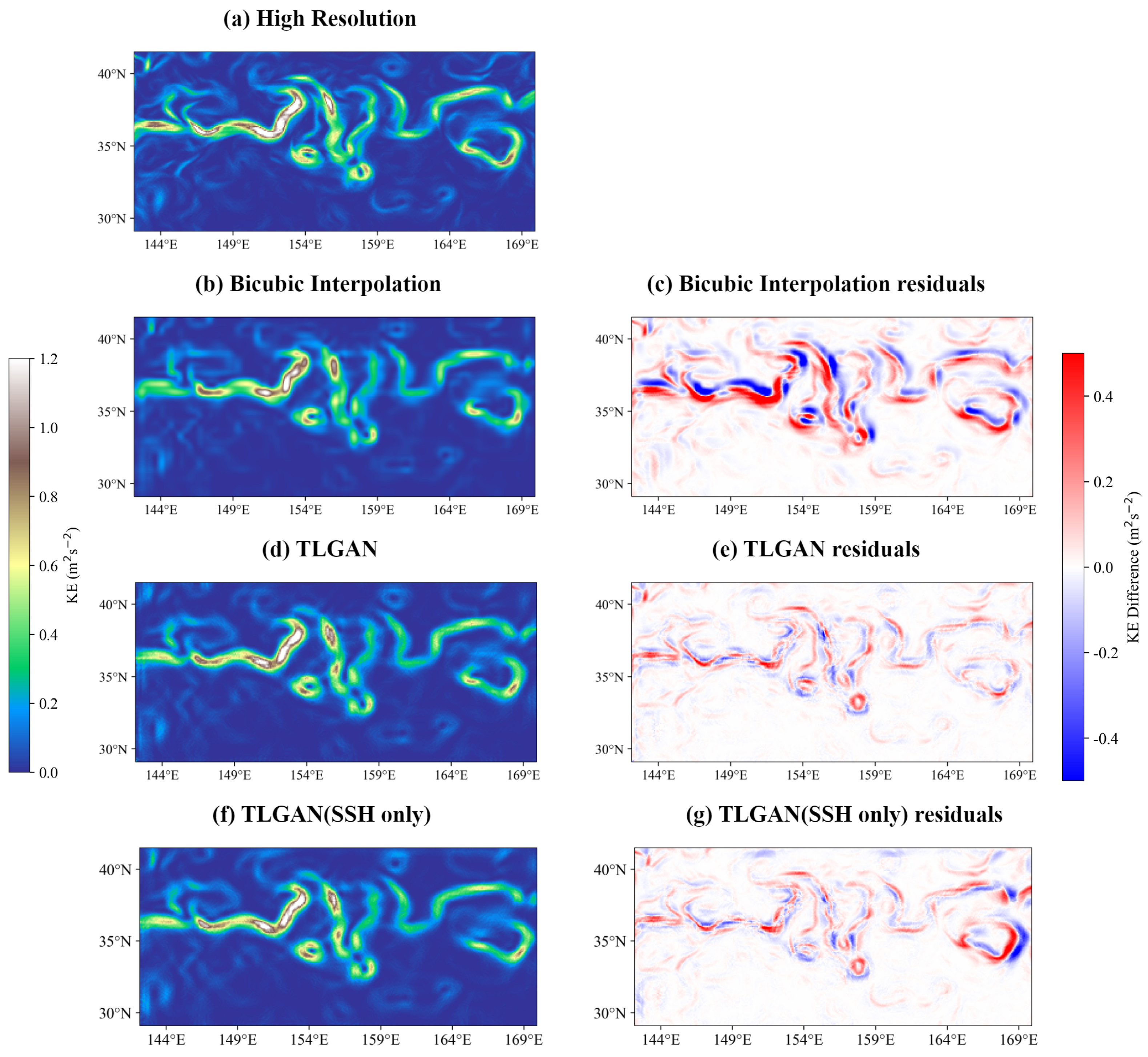
The SSH data find extensive application in estimating the kinetic energy (KE) and the geostrophic currents field within ocean circulation [30,31]. Figure 3 illustrates an instance of KE fields derived from high-resolution SSH data and reconstructed super-resolution SSH data. Notably, Figure 3c reveals that bicubic interpolation tends to underestimate the KE of the Kuroshio Extension front at the 0.5 level. This discrepancy is mitigated by TLGAN, reducing the error to less than 0.2. This improvement is particularly evident at the edges where strong currents are associated. The TLGAN reconstruction effectively enhances gradients that were smoothed out by bicubic interpolation, as observed in Figure 3. A noteworthy comparison is made between TLGAN and TLGAN (SSH only). The inclusion of SST data contributes to obtaining more accurate KE information. This enhancement is attributed to the ability of SST data to provide additional context and improve the fidelity of the reconstructed kinetic energy fields.

To assess the impact of geostrophic flow estimation, we computed the complex correlation between the velocities derived from both bicubic interpolation and TLGAN models and the velocities from the original fields. Complex correlation, employed in various oceanographic studies for two-dimensional vector analysis, is demonstrated in previous works [32,33,34,35]. As outlined in

Table 2. Complex correlation between the geostrophic currents computed from the reconstructed SSH fields by bicubic interpolation and TLGAN models.

Model	Complex Correlation
	min.	max.	mean.	sth.
Bicubic Interpolation	0.740	0.799	0.767	0.011
TLGAN(SSH+${\mathrm{SST}}_{\mathrm{m}12}$)	0.934	0.954	0.943	0.005
TLGAN(SSH+${\mathrm{SST}}_{\mathrm{m}6}$)	0.908	0.955	0.937	0.010
TLGAN(SSH only)	0.632	0.707	0.669	0.022

, it is evident that bicubic interpolation exhibits considerably poorer performance compared to TLGAN models. Furthermore, a comparative analysis of different TLGAN training configurations, involving varying amounts of SST data, reveals a significant contribution of SST data. This is highlighted by an improvement in mean values from 0.67 to 0.94, emphasizing the notable enhancement in performance associated with the inclusion of SST data in TLGAN training.

5. Discussion

SSH and SST exhibit a complex dynamical relationship. Deep learning methods can learn to exploit these relationships without being restricted to specific times and regions. Previous studies have shown that combining SSH and SST data can lead to the better detection of abnormal eddies compared to using solo data sources [36]. Additionally, the synergy of SSH and SST data has been employed to detect and recognize small-scale eddy-front associations, with including SST resulting in lower reconstruction errors than SSH observations alone [37]. Our study demonstrates that deep learning can overcome the limitations of paired SSH-SST datasets. Leveraging transfer learning, we can input SSH and SST data into the deep learning model separately, allowing the model to learn the rules of data changes and fuse these features in the same latent space, thus enhancing flexibility in research.

The TLGAN architecture demonstrates an innovative approach by dividing training into multiple stages, facilitating the fusion of heterogeneous datasets. Enhancing the accuracy of TLGAN can be achieved through training with an extended dataset spanning several years instead of just one. Furthermore, exploring additional attempts such as training distinct TLGAN models for various geographical regions may further enhance the model performance. This study serves as a feasibility analysis for designing a prospective operational deep learning method tailored specifically for downsizing the SSH domain. Notably, the TLGAN model training leverages ocean model outputs of exceptionally high resolution, enabling the acquisition of detailed data that surpass the capabilities of in-situ measurements. However, the complexity of real-world scenarios presents a formidable challenge. When working with actual satellite data, it becomes imperative to account for factors such as SSH sampling along the satellite orbit across multiple time periods and the intricate spatiotemporal interpolation of altimeter data. The errors observed in the final satellite product stem not from mere smoothing but from the complex nature of spatiotemporal interpolation. Addressing this multifaceted challenge necessitates further advancements in developing efficient operational deep learning algorithms, a task that extends beyond the scope of this article.

6. Conclusions

In this study, we introduce a novel TLGAN model designed for reconstructing high-resolution SSH fields by incorporating heterogeneous SST data. The proposed model features a new generator network comprising three blocks to efficiently extract deep features from both SSH and SST data in the latent space. We employ a hybrid strategy involving adversarial training and transfer learning to reconstruct the super-resolution field. This demonstrates the consistent superiority of the TLGAN model over the bicubic interpolation method, as substantiated by both visual inspection and objective metrics. Additionally, we confirm that the fusion of additional SST information into SSH reconstruction excels in producing more accurate downscaling of SSH fields and dynamic quantities such as eddy kinetic energy and surface geostrophic currents.

References

1. Pascual, A.; Faugère, Y.; Larnicol, G.; Le Traon, P.Y. Improved description of the ocean mesoscale variability by combining four satellite altimeters. Geophys. Res. Lett. 2006, 33, L02611. [Google Scholar] [CrossRef]
2. Dufau, C.; Orsztynowicz, M.; Dibarboure, G.; Morrow, R.; Le Traon, P.Y. Mesoscale resolution capability of altimetry: Present and future. J. Geophys. Res. Ocean. 2016, 121, 4910–4927. [Google Scholar] [CrossRef]
3. Kalluri, S.; Cao, C.; Heidinger, A.; Ignatov, A.; Key, J.; Smith, T. The Advanced Very High Resolution Radiometer: Contributing to Earth Observations for over 40 Years. Bull. Am. Meteorol. Soc. 2021, 102, 351–366. [Google Scholar] [CrossRef]
4. Tandeo, P.; Chapron, B.; Ba, S.; Autret, E.; Fablet, R. Segmentation of Mesoscale Ocean Surface Dynamics Using Satellite SST and SSH Observations. IEEE Trans. Geosci. Remote Sens. 2014, 52, 4227–4235. [Google Scholar] [CrossRef]
5. Le Goff, C.; Fablet, R.; Tandeo, P.; Autret, E.; Chapron, B. Spatio-temporal decomposition of satellite-derived SST–SSH fields: Links between surface data and ocean interior dynamics in the Agulhas region. IEEE J. Sel. Top. Appl. Earth Obs. Remote Sens. 2016, 9, 5106–5112. [Google Scholar] [CrossRef]
6. González-Haro, C.; Isern-Fontanet, J.; Tandeo, P.; Garello, R. Ocean surface currents reconstruction: Spectral characterization of the transfer function between SST and SSH. J. Geophys. Res. Ocean. 2020, 125, e2019JC015958. [Google Scholar] [CrossRef]
7. Ciani, D.; Rio, M.H.; Nardelli, B.B.; Etienne, H.; Santoleri, R. Improving the altimeter-derived surface currents using sea surface temperature (SST) data: A sensitivity study to SST products. Remote Sens. 2020, 12, 1601. [Google Scholar] [CrossRef]
8. Buongiorno Nardelli, B.; Cavaliere, D.; Charles, E.; Ciani, D. Super-resolving ocean dynamics from space with computer vision algorithms. Remote Sens. 2022, 14, 1159. [Google Scholar] [CrossRef]
9. Martin, S.A.; Manucharyan, G.E.; Klein, P. Synthesizing sea surface temperature and satellite altimetry observations using deep learning improves the accuracy and resolution of gridded sea surface height anomalies. J. Adv. Model. Earth Syst. 2023, 15, e2022MS003589. [Google Scholar] [CrossRef]
10. Thiria, S.; Sorror, C.; Archambault, T.; Charantonis, A.; Bereziat, D.; Mejia, C.; Molines, J.M.; Crépon, M. Downscaling of ocean fields by fusion of heterogeneous observations using deep learning algorithms. Ocean Model. 2023, 182, 102174. [Google Scholar] [CrossRef]
11. Archambault, T.; Charantonis, A.; Béréziat, D.; Mejia, C.; Thiria, S. Sea surface height super-resolution using high-resolution sea surface temperature with a subpixel convolutional residual network. Environ. Data Sci. 2022, 1, e26. [Google Scholar] [CrossRef]
12. Dong, C.; Loy, C.C.; He, K.; Tang, X. Image super-resolution using deep convolutional networks. IEEE Trans. Pattern Anal. Mach. Intell. 2015, 38, 295–307. [Google Scholar] [CrossRef]
13. Yang, W.; Zhang, X.; Tian, Y.; Wang, W.; Xue, J.H.; Liao, Q. Deep learning for single image super-resolution: A brief review. IEEE Trans. Multimed. 2019, 21, 3106–3121. [Google Scholar] [CrossRef]
14. Wang, P.; Bayram, B.; Sertel, E. A comprehensive review on deep learning based remote sensing image super-resolution methods. Earth-Sci. Rev. 2022, 232, 104110. [Google Scholar] [CrossRef]
15. Sdraka, M.; Papoutsis, I.; Psomas, B.; Vlachos, K.; Ioannidis, K.; Karantzalos, K.; Gialampoukidis, I.; Vrochidis, S. Deep learning for downscaling remote sensing images: Fusion and super-resolution. IEEE Geosci. Remote Sens. Mag. 2022, 10, 202–255. [Google Scholar] [CrossRef]
16. Chen, H.; He, X.; Qing, L.; Wu, Y.; Ren, C.; Sheriff, R.E.; Zhu, C. Real-world single image super-resolution: A brief review. Inf. Fusion 2022, 79, 124–145. [Google Scholar] [CrossRef]
17. Ledig, C.; Theis, L.; Huszar, F.; Caballero, J.; Cunningham, A.; Acosta, A.; Aitken, A.; Tejani, A.; Totz, J.; Wang, Z.; et al. Photo-Realistic Single Image Super-Resolution Using a Generative Adversarial Network. In Proceedings of the IEEE Conference on Computer Vision and Pattern Recognition (CVPR), Honolulu, HI, USA, 21–26 July 2017. [Google Scholar]
18. Wang, J.; Liu, Z.; Foster, I.; Chang, W.; Kettimuthu, R.; Kotamarthi, V.R. Fast and accurate learned multiresolution dynamical downscaling for precipitation. Geosci. Model Dev. 2021, 14, 6355–6372. [Google Scholar] [CrossRef]
19. Huang, Y.; Jiang, Z.; Lan, R.; Zhang, S.; Pi, K. Infrared image super-resolution via transfer learning and PSRGAN. IEEE Signal Process. Lett. 2021, 28, 982–986. [Google Scholar] [CrossRef]
20. Stengel, K.; Glaws, A.; Hettinger, D.; King, R.N. Adversarial super-resolution of climatological wind and solar data. Proc. Natl. Acad. Sci. USA 2020, 117, 16805–16815. [Google Scholar] [CrossRef]
21. Simonyan, K.; Zisserman, A. Very deep convolutional networks for large-scale image recognition. arXiv 2014, arXiv:1409.1556. [Google Scholar]
22. Zhang, Y.; Tian, Y.; Kong, Y.; Zhong, B.; Fu, Y. Residual dense network for image super-resolution. In Proceedings of the IEEE Conference on Computer Vision and Pattern Recognition, Salt Lake City, UT, USA, 18–23 June 2018; pp. 2472–2481. [Google Scholar]
23. Liu, J.; Tang, J.; Wu, G. Residual feature distillation network for lightweight image super-resolution. In Proceedings of the Computer Vision–ECCV 2020 Workshops, Glasgow, UK, 23–28 August 2020; Proceedings, Part III 16. pp. 41–55. [Google Scholar]
24. Shi, W.; Caballero, J.; Huszár, F.; Totz, J.; Aitken, A.P.; Bishop, R.; Rueckert, D.; Wang, Z. Real-time single image and video super-resolution using an efficient sub-pixel convolutional neural network. In Proceedings of the IEEE Conference on Computer Vision and Pattern Recognition, Las Vegas, NV, USA, 27–30 June 2016; pp. 1874–1883. [Google Scholar]
25. Jean-Michel, L.; Eric, G.; Romain, B.B.; Gilles, G.; Angélique, M.; Marie, D.; Clément, B.; Mathieu, H.; Olivier, L.G.; Charly, R.; et al. The Copernicus global 1/12 oceanic and sea ice GLORYS12 reanalysis. Front. Earth Sci. 2021, 9, 698876. [Google Scholar] [CrossRef]
26. Ji, J.; Dong, C.; Zhang, B.; Liu, Y. An oceanic eddy statistical comparison using multiple observational data in the Kuroshio Extension region. Acta Oceanol. Sin. 2017, 36, 1–7. [Google Scholar] [CrossRef]
27. Sun, W.; An, M.; Liu, J.; Liu, J.; Yang, J.; Tan, W.; Dong, C.; Liu, Y. Comparative analysis of four types of mesoscale eddies in the Kuroshio-Oyashio extension region. Front. Mar. Sci. 2022, 9, 984244. [Google Scholar] [CrossRef]
28. Singla, K.; Pandey, R.; Ghanekar, U. A review on Single Image Super Resolution techniques using generative adversarial network. Optik 2022, 266, 169607. [Google Scholar] [CrossRef]
29. Wang, X.; Xie, L.; Yu, K.; Chan, K.C.; Loy, C.C.; Dong, C. BasicSR: Open Source Image and Video Restoration Toolbox; GitHub: San Francisco, CA, USA, 2022. [Google Scholar]
30. Liu, Y.; Chen, G.; Sun, M.; Liu, S.; Tian, F. A Parallel SLA-Based Algorithm for Global Mesoscale Eddy Identification. J. Atmos. Ocean. Technol. 2016, 33, 2743–2754. [Google Scholar] [CrossRef]
31. Yu, P.; Zhang, L.; Liu, M.; Zhong, Q.; Zhang, Y.; Li, X. A comparison of the strength and position variability of the Kuroshio Extension SST front. Acta Oceanol. Sin. 2020, 39, 26–34. [Google Scholar] [CrossRef]
32. Poulain, P.M.; Gerin, R.; Mauri, E.; Pennel, R. Wind effects on drogued and undrogued drifters in the eastern Mediterranean. J. Atmos. Ocean. Technol. 2009, 26, 1144–1156. [Google Scholar] [CrossRef]
33. Poulain, P.M.; Menna, M.; Mauri, E. Surface geostrophic circulation of the Mediterranean Sea derived from drifter and satellite altimeter data. J. Phys. Oceanogr. 2012, 42, 973–990. [Google Scholar] [CrossRef]
34. Menna, M.; Poulain, P.M. Geostrophic currents and kinetic energies in the Black Sea estimated from merged drifter and satellite altimetry data. Ocean Sci. 2014, 10, 155–165. [Google Scholar] [CrossRef]
35. Röhrs, J.; Christensen, K.H. Drift in the uppermost part of the ocean. Geophys. Res. Lett. 2015, 42, 10349–10356. [Google Scholar] [CrossRef]
36. Liu, Y.; Zheng, Q.; Li, X. Characteristics of global ocean abnormal mesoscale eddies derived from the fusion of sea surface height and temperature data by deep learning. Geophys. Res. Lett. 2021, 48, e2021GL094772. [Google Scholar] [CrossRef]
37. Ma, Y.; Tian, F.; Long, S.; Huang, B.; Liu, W.; Chen, G. Global Oceanic Eddy-Front Associations from Synergetic Remote Sensing Data by Deep Learning. IEEE Geosci. Remote Sens. Lett. 2023, 20, 1503005. [Google Scholar] [CrossRef]
Figure 1. The details of proposed TLGAN model, (a) generator architecture, and (b) basic block diagram of SRGAN method.
Remotesensing 16 00763 g001aRemotesensing 16 00763 g001b
Figure 2. Some examples showcasing the super resolution reconstruction results. The left column corresponds to the data from February 2020, while the right column corresponds to the data from October 2020.
Remotesensing 16 00763 g002
Figure 3. Comparison of kinetic energy outputs of the models based on one day data of October 2020.
Remotesensing 16 00763 g003