A Geographic Object-Based Image Approach Based on the Sentinel-2 Multispectral Instrument for Lake Aquatic Vegetation Mapping: A Complementary Tool to In Situ Monitoring

Abstract

Aquatic vegetation is an essential component of lake ecosystems, used as a biological indicator for in situ monitoring within the Water Framework Directive. We developed a hierarchical object-based image classification model with multi-seasonal Sentinel-2 imagery and suitable spectral indices in order to map the aquatic vegetation in a Mediterranean oligotrophic/mesotrophic deep lake; we then applied the model to another lake with similar abiotic and biotic characteristics. Field data from a survey of aquatic macrophytes, undertaken on the same dates as EO data, were used within the accuracy assessment. The aquatic vegetation was discerned into three classes: emergent, floating, and submerged aquatic vegetation. Geographic object-based image analysis (GEOBIA) proved to be effective in discriminating the three classes in both study areas. Results showed high effectiveness of the classification model in terms of overall accuracy, particularly for the emergent and floating classes. In the case of submerged aquatic vegetation, challenges in their classification prompted us to establish specific criteria for their accurate detection. Overall results showed that GEOBIA based on spectral indices was suitable for mapping aquatic vegetation in oligotrophic/mesotrophic deep lakes. EO data can contribute to large-scale coverage and high-frequency monitoring requirements, being a complementary tool to in situ monitoring.

1. Introduction

Inland water ecosystems are significant because of the high biodiversity and endemism they support [1,2] and the variety of valuable ecosystem services they provide [3]. However, they suffer from rapid habitat loss and degradation at a global scale [4,5]. In particular, in recent decades and under intensified climate pressure, the quality of inland waters has been severely threatened and often dramatically degraded [4]; thus, the monitoring of bio-physical variables depicting water conditions became essential [6]. Water quality monitoring was based for many years on in situ measurements, allowing the collection of data for an extensive set of biotic and abiotic parameters (e.g., nutrient concentrations, phytoplankton abundance, aquatic vegetation richness and abundance). These constituent parameters eventually became subject to national and international standards [7,8,9]. Over the last few years, the biomonitoring of European aquatic ecosystems changed substantially to reflect aquatic structure and functioning [10]. The development was driven by the EU Water Framework Directive 2000/60/EC (WFD) [11], according to which WFD-compliant monitoring and assessment methods have been developed by Member States [12].

Aquatic vegetation is an integral part of lake ecosystems, playing a significant role in their structure and functioning (e.g., by providing habitat for species, stabilizing sediments, helping the migration and circulation of elements, improving water quality, and limiting the growth of algae) [13,14,15,16]. This role is critical for the evolution, ecological balance, and restoration of lakes. Aquatic plants (hydrophytes or macrophytes) in lakes can be divided into three groups, namely emergent aquatic vegetation (EAV); floating aquatic vegetation (FAV), comprising two subclasses (free-floating and floating-leaved macrophytes); and submerged aquatic vegetation (SAV). Among them, EAV and FAV are above the water surface, while SAV is below the water surface. Each species of aquatic vegetation has its unique ecological function [17,18,19]. SAV is especially related to water transparency, water depth, and eutrophication, and its biomass is usually considered a key indicator for evaluating the quality of lake ecosystems [20]. Changes in the composition and abundance, such as a decline in submerged vegetation and an increase in abundance of free-floating plants [21], indicate the degradation of lake ecosystems [17,22]. Thus, aquatic macrophytes are widely used as a biological indicator in monitoring and assessment systems developed in the context of WFD for lakes [19,23]. Moreover, the monitoring of temporal and spatial patterns of the growth status and the distribution of aquatic vegetation, in relation to environmental factors, is of great significance, especially considering its role in the ecological restoration of lake ecosystems [24,25].

More than 20 years after the adoption of WFD, the need for innovation in monitoring is highlighted [26], together with the requirement to provide sufficient spatial and temporal resolution and, in some cases, to make monitoring more cost-effective [26] or to address some of the limitations of in situ methods [27,28,29]. The rapid, large-scale, and regular monitoring of aquatic vegetation via remote sensing is essential in order to improve the dynamic monitoring of aquatic vegetation [30]. Additionally, it enhances confidence in WFD classification through increasing both the spatial coverage and frequency of monitoring variables such as macrophyte coverage [26,31]. Moreover, remote sensing products can be used in quantitative analysis and compared over time, showing the progressive changes in such ecosystems [28]. However, mapping the spatial extent of aquatic vegetation has proven to be a challenging task, due to the complexity of aquatic systems, in terms of high temporal variability, heterogeneity in optical response through water column attenuation, and due to lack of available data [30]. In particular, several factors, such as the physiological status of vegetation, stress, or diseases, can lead to alterations in the spectral response of the vegetation [32]. Because of the wide spectral variability, the classification of aquatic vegetation can often lead to poor results.

As remote sensing technologies are rapidly evolving, a range of studies utilizing different satellite data and extraction methods for aquatic vegetation mapping have been developed with remarkable results [20,28,33,34,35,36,37,38]. In particular, the use of multiseasonal imagery in order to incorporate seasonal variability in water regimes and vegetation phenology, is considered very helpful [33,34,37,39]. For instance, Ramsey and Laine [40] demonstrated that the combination of images from two seasons facilitates segregation between emergent and floating vegetation (winter and spring), and between flooded emergent vegetation and open water (autumn and winter). However, commercial spaceborne or airborne data are prohibitively expensive for large-scale and regular monitoring, which often results in annual and intra-annual data gaps. Thus, Sentinel-2 sensors are an attractive contender to monitor the rapid expansion of macrophytes during the growing season, due to their high revisit frequency and spectral resolution [41]. Although they are not as powerful in terms of spectral resolution as hyperspectral data, or their spatial resolution is not as detailed as very-high-resolution (VHR) data or UAV–acquired data, multispectral data, such as those from Sentinel-2, offer a high degree of flexibility and applicability for macrophyte mapping and monitoring at larger scales [42,43].

Alternative image classification algorithms, such as decision tree [44,45] or neural network classifiers [46], have been widely used in aquatic vegetation mapping. For example, Zhao et al. [47] and Luo et al. [34,48] utilized Landsat TM and HJ-CCD imagery, respectively, to develop a decision tree algorithm for the detection of emergent, floating, and submerged aquatic vegetation in Taihu Lake. The study of Rodriquez—Garlito [46] incorporates spectral indices from Sentinel-2 band combinations with a convolutional neural network classifier, in order to detect invasive aquatic plants. Villa et al. [49] developed a rule-based classification scheme for mapping aquatic vegetation types, based on vegetation indices with consistent accuracy results. De Grandpe et al. [50] utilized an object-based image analysis workflow, incorporating spectral indices, in order to generate SAV cover maps in complex aquatic environments. Visser et al. [51] applied multi-level object-based image analysis combined with expert knowledge to obtain consistent classifications of SAV in shallow clear-water streams. Geographic object-based image analysis (GEOBIA) offers a framework that can be used to integrate more complex data than the raw remote sensing signal by including different levels of spatial information related to scale, shape, and texture [50,52,53,54]. This higher level of information offers a more robust comparative basis than pixel-based approaches when radiometric accuracy is uncertain, such as in complex water cases.

In this study, we test whether the multi-seasonal observation capability of large-scale, open-source Sentinel-2MSI provides sufficient information for aquatic vegetation mapping, potentially supporting in situ monitoring according to WFD, in Mediterranean oligotrophic/mesotrophic deep lakes. In particular, we develop a GEOBIA classification model based on spectral indices, which are better suited to monitor aquatic vegetation; this way, we both ensure the simplicity of a spectral index (SI)-based approach and aim at efficiency in monitoring aquatic vegetation. Our main objectives are as follows: (i) to develop a hierarchical object-based classification model based mainly on SIs for aquatic vegetation mapping in an oligotrophic–mesotrophic deep lake and to apply it in a second lake with similar characteristics; (ii) to test its accuracy in two Mediterranean lakes. Thus, we evaluate its effectiveness through reference data and assess its overall applicability for similar lakes.

2. Materials and Methods

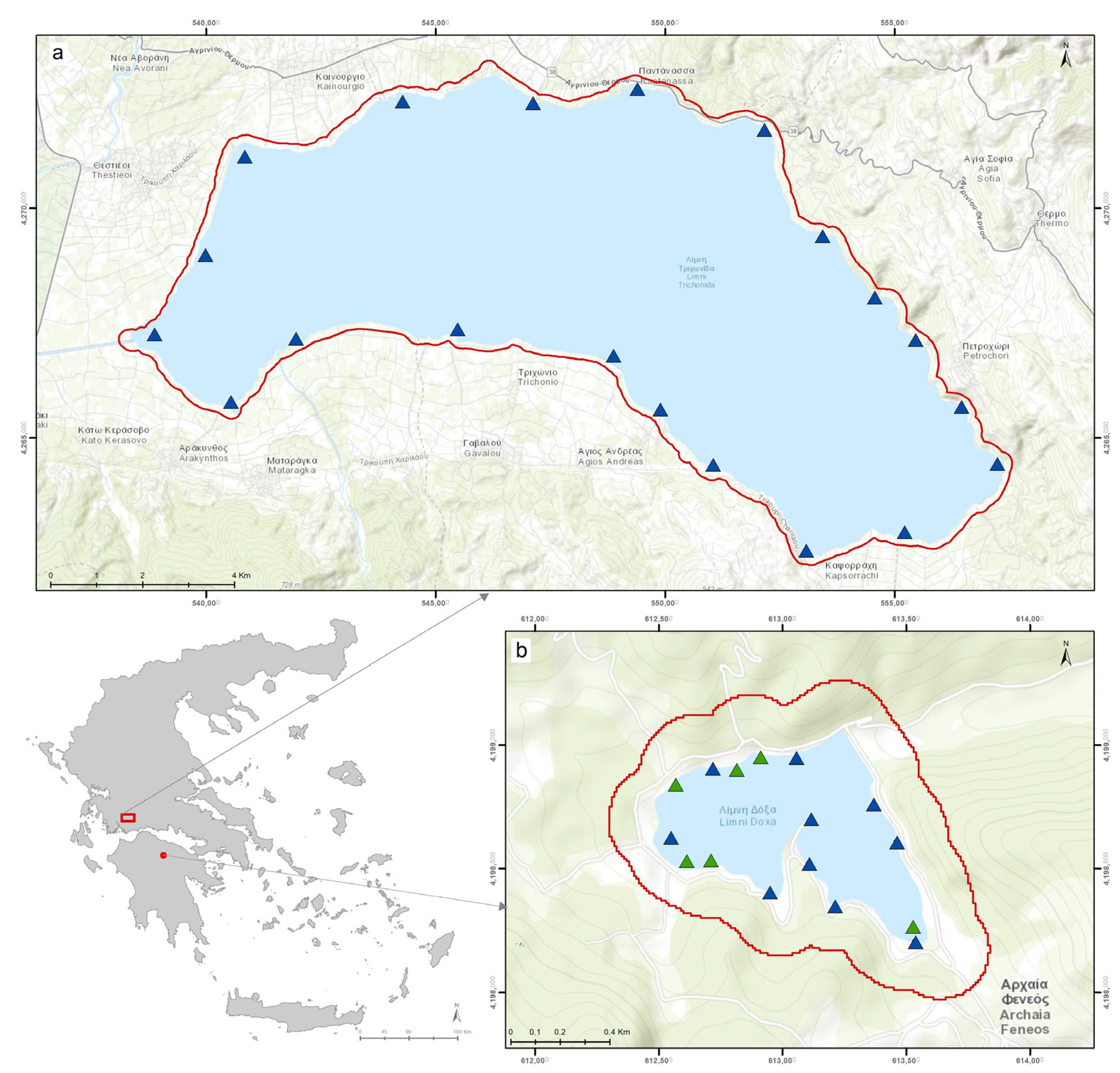
2.1. Site Description

We developed and tested our approach for the classification of aquatic vegetation in two freshwater lakes, featuring high abundances of aquatic vegetation: Trichonida Lake and Feneos Lake, Greece (Figure 1). Both lakes are part of the National Monitoring Network of Waters in Greece (see http://nmwn.ypeka.gr/, (accessed on 15 September 2022) and https://wfd.ekby.gr/, accessed on (15 September 2022) for details) and they have been monitored by The Goulandris Natural History Museum—Greek Biotope/Wetland Centre (EKBY), since 2012 [55].

Trichonida Lake (38°34′21″ N 21°33′09″ E) is the deepest and largest natural lake in Greece, located 16 m above the mean sea level in the eastern area of Aetolia-Acarnania (Figure 1a). The lake covers an area of approximately 96 km² (up to 19 km long and 6 km wide), stretching in the W–E direction, and its maximum depth is 52 m [56]. According to the updated Köppen–Geiger classification [57], the lake is located in a Csa climate zone, which is defined as a warm temperate climate with hot and dry summers. Trichonida Lake is one of the seven warm monomictic deep natural lakes with a mean depth > 9 m (national type Deep Natural Lake (GR-DNL)) of the Greek National Water Monitoring Network [58]. It is connected to Lysimachia Lake through a narrow superficial long canal (2.8 km) located at its western part. The lake plays an important role in flood management, drought prevention, carbon sequestration, biodiversity maintenance, and microclimate regulation. Although we have not conducted a hydrological analysis of the lake, there are a few studies available on hydroclimatic variables’ temporal trends [59,60,61] as well as the lake’s biological parameters [62,63,64,65,66]. The lake and its surrounding area is part of the European Natura 2000 network of protected sites as a Special Area for Conservation (code GR2310009), as it hosts types of habitats and species of European interest [67]. Although it was characterized as an oligotrophic lake more than 40 years ago [68,69] the presence of vascular plants such as Myriophyllum spicatum, Potamogeton pectinatus, Ranunculus trichophyllus, and others that mostly occur in eutrophic or mesotrophic lakes [70] indicate its mesotrophic tendencies. This is consistent with the results of the ecological classification of the lake in good ecological status (from 2013 to 2021), according to the WFD-compliant national monitoring and assessment method (HeLM) based on aquatic macrophytes [23]. Aquatic plants recorded in the lake were grouped as emergent aquatic vegetation, floating aquatic vegetation, and submerged aquatic vegetation. The dominant species of each vegetation type, as recorded by the samplings undertaken by the National Monitoring Network, are presented in

Table 1. Types of aquatic vegetation in Trichonida and Feneos Lakes.

Vegetation Type	Dominant Species
	Trichonida Lake	Feneos Lake
EAV (emergent aquatic vegetation)	Phragmites australis Bolboschoenus maritimus Schoenoplectus litoralis	Typha angustifolia Phragmites australis
FAV (floating aquatic vegetation)	Ludwigia peploides Nymphaea alba	-
SAV (submerged aquatic vegetation)	Vallisneria spiralis Ceratophyllum demersum Myriophyllum spicatum Najas marina	Chara vulgaris Myriophyllum spicatum Nitella flexilis Nitella furcata Vallisneria spiralis

.

Feneos Lake (37°55′45″N 22°17′11″E) is an artificial lake, located 872 m above sea level in the area of western Corinthia in the Peloponnese (Figure 1b). It covers a mean surface of 0.5 km² with a maximum depth of 29 m. As per the updated Köppen–Geiger classification, the area is categorized under the Csb climate zone, which is defined as a temperate climate with warm summers [57]. Even though it is an artificial lake constructed in the mid-1990s for storage purposes, it resembles a natural lake as a species-rich abundant aquatic vegetation has been developed due to absence of water abstraction and to natural water level fluctuation [23]. Its ecological status is characterized as “High” for the period 2013–2021, based on the HeLM system. The lake is surrounded by Mediterranean pine forests with endemic black pines and lacks any pollution sources. The lake and its surrounding area are part of a wider area included in the European Natura 2000 network of protected areas (GR2320002, GR2320013). Over the years, it has developed into an important ecotourism attraction. Additionally, only non-motorboat activities are allowed in the lake for recreational purposes. Aquatic plant species recorded by the samplings undertaken by the National Monitoring Network were grouped into two types, i.e., emergent aquatic vegetation and submerged aquatic vegetation. The dominant species per vegetation type are presented in Table 1. A buffer zone of 200 m (red polygon boundary in Figure 1) was generated around the lakeshore in both lakes. This was decided in order to detect all potential locations of aquatic vegetation due to water level fluctuations and to provide some additional information regarding the surrounding cover area. The respective shoreline was determined based on the average water level of 2021, which was 16 m above the mean sea level for Trichonida Lake and 872 m above the mean sea level for Feneos Lake. The final study areas cover 10,495 ha and 130 ha for Trichonida and Feneos lakes, respectively.

The lakes do not form an integrated hydrological system and the geomorphology of their basin is differentiated, leading also to different morphometric characteristics. However, they have common characteristics regarding mainly the water transparency. Their vegetation has also some similarities (e.g., there are extended patches of Vallisneria spiralis and Myriophyllum spicatum dominated communities) but also different macrophytic communities such as the Characeae communities in the deeper parts of the littoral zone in Feneos Lake, or the Ceratophyllum demersum- and Najas marina-dominated communities in Trichonida Lake. We believe that these similarities, but also the differentiations in the biotic and abiotic characteristics, make these two lakes a suitable pair to develop and test our methodology.

2.2. Datasets

2.2.1. In Situ Monitoring Data of Aquatic Vegetation

With regard to the monitoring and assessment system applied for the implementation of the WFD (HelM [23]), a full survey of aquatic macrophytes is undertaken every three years at each lake of the national network (Trichonida and Feneos lakes amongst them), while the maximum colonization depth (C_max) of the aquatic vegetation is measured per lake per year.

The sampling method consists of establishing belt transects perpendicular to the lake’s shoreline, which are revisited in each sampling survey. They are linearly arranged with a length extending from the shoreline to the maximum depth of plant growth and a width of approximately 5 m. In these transects, the taxonomic composition of aquatic macrophytes is recorded in five depth zones, 0–1 m, 1–2 m, 2–4 m, 4–8 m, and >8 m (consisting the individual surveying plots), and their abundance is estimated on the semi-quantitative five-point DAFOR scale [71,72] (for details on the sampling method, see [23]). In each depth zone, five sampling points, evenly distributed along the increasing depth gradient, are determined. In Trichonida Lake, 20 belt transects have been established with 42 plots on average per transect. In Lake Feneos, 10 transects have been established due to its small area, with 32 plots on average per transect. The number of plots per transect varies due to the variation in C_max among the different transects. The last field survey in both lakes was carried out in August 2021. Additional plots (of an area of 5 × 5 m) were sampled in August 2022 in Feneos Lake (green points in Figure 1).

In order to effectively extract the information from these plots in the current study, sorting was required, especially as these plots were both distributed in dense linear patches along the transects and covered by more than one vegetation type. In particular, plots were carefully chosen from the initial field dataset, with the criterium of vegetation cover >80% of one of the studied classes (EAV, FAV, SAV). In the end, we selected 110 plots in total (64 for Trichonida Lake and 46 for Feneos Lake). A point was generated per plot and then attributed to the corresponding class. The generated points were used throughout the accuracy assessment process.

2.2.2. Bathymetric Data

The bathymetric data we used are contour lines derived from corresponding bathymetric Digital Elevation Models (DEMs). They were developed within the National Monitoring Network of Waters in Greece by EKBY [56] and are available at EKBY’s Geoserver [73]. They were produced by the following methods: (i) bathymetry measurements using sonar and GPS on a floating medium; (ii) digitization of contours and elevation points in the littoral nearshore area from 1:5000 scale topographic maps, where the equi-dimensionality of the contours was 2 m and the accuracy of the elevation points was 2 cm; (iii) interpolation of the above data to produce very-high-resolution (1 m pixel size) DEMs. The “Topo to Raster” tool is available in ESRI ArcGIS software v. 10.8.2. and is based on the ANUDEM program developed by Michael Hutchinson [74,75,76,77,78]. These data were used in order to determine the shoreline and the respective buffer zones and to assist in outlining deep water areas as well.

2.2.3. Satellite Data

In this study, Sentinel 2A-MSI L2A products were employed, available freely from the Copernicus Data Space Ecosystem [79]. They are distributed as ortho-rectified and UTM-geocoded bottom-of-atmosphere (BOA) reflectance images. Τhe Sentinel-2A carries on board the MultiSpectral Instrument (MSI) optical sensor, which acquires images in 13 bands (spectral region between 442 and 2201 nm) with a spatial resolution of 10, 20, and 60 m (depending on the spectral band) (

Table 2. Spectral parameters of Sentinel-2 satellite images and data acquisition dates.

Sentinel 2_MSI Bands	Central Wavelength (μm)	Resolution (m)	Trichonida Lake	Feneos Lake
Band 1—Coastal aerosol	0.443	60	17-February-21 (ws) 12-July-21 (ss)	27-February-21 (ws) 27-July-21 (ss)
Band 2—Blue	0.490	10
Band 3—Green	0.560	10
Band 4—Red	0.665	10
Band 5—Veg. Red Edge	0.705	20
Band 6—Veg. Red Edge	0.740	20
Band 7—Veg. Red Edge	0.783	20
Band 8—NIR	0.842	10
Band 8A—Veg. Red Edge	0.865	20
Band 9—Water vapour	0.945	60
Band 10—SWIR Cirrus	1.375	60
Band 11—SWIR1	1.610	20
Band 12—SWIR2	2.190	20

) [80]. For this study, the 10 bands of the VIS–NIR and SWIR region (b2–b8A and b11–b12) were stacked into a single file resampled to a 10 m spatial resolution. As the atmospheric correction is a key limiting factor of satellite-based water quality monitoring, the reliability of results from water-leaving reflectance will be subject to the quality of atmospheric correction [81]. We used the Sentinel-2 Level 2 products, which are atmospherically corrected with the SEN2COR package, since this method, as used in many similar studies, was found to be more suitable for the correction of inland water bodies compared to coastal areas [81,82]. Therefore, two tiles per study area were acquired, one for the summer season (ss) and one for the winter season (ws) (Table 2), in order to incorporate the highest temporal phenological differentiation of the aquatic vegetation in the analysis. The dates for the summer season were chosen in relevance to the dates of the in situ macrophyte survey. Cloud cover was <15%; thus, cloud masking was not required.

It should be noted that the Sentinel-2 data were not further processed for water body correction. This was decided since it has been demonstrated that Sentinel-2 data can achieve benthic substrate differentiation through atmospheric correction only [83]. Additionally, other studies have concluded that water column correction models, based on band combination, provide only minor improvements in calm, clear, and shallow waters, while their use is discouraged in complex and deep areas [84]. Moreover, there are also difficulties with their transferability to other image acquisitions with different conditions [84]. It is worth pointing out that other studies demonstrate satisfactory results, obtained without applying water column correction [85,86,87].

2.3. Study Workflow

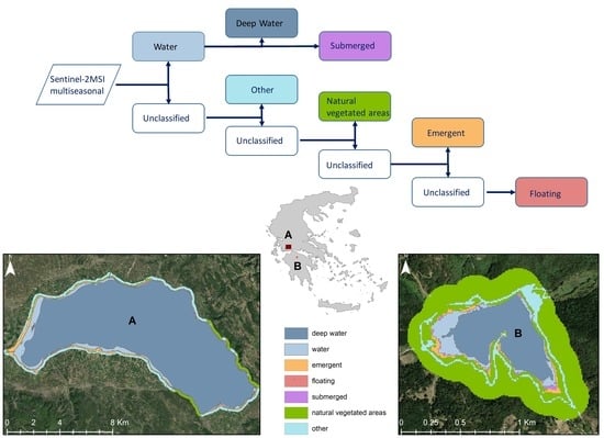
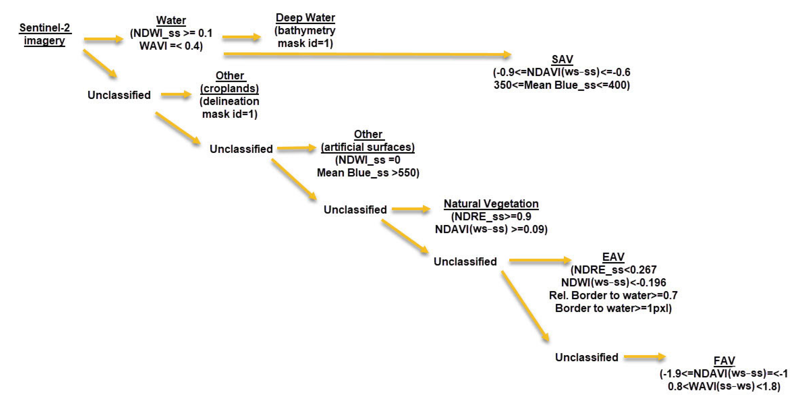
2.3.1. Classification Scheme

Since the analysis was based on the optical response of aquatic vegetation from Earth Observation (EO) data with the above-mentioned specific spectral and spatial characteristics (Table 2), the classification scheme should take into account the capabilities of the input satellite data in capturing macrophyte heterogeneity. As an example, SAV can be effectively mapped from EO medium resolution data when they present enough density, even in cases of mixture with other species such as floating [49]. Moreover, the discrimination of macrophyte classes with a mixed presence with no clear dominance, and/or of small patches of such communities, is impossible from multi-spectral satellite data at a medium spatial resolution (10–30 m), particularly in small water systems [49].

Considering all that was mentioned above, we used a comprehensive classification scheme that could potentially be feasible to map. We used the grouped aquatic vegetation types (i) “Emergent” (EAV), (ii) “Floating” (FAV), and (iii) “Submerged” (SAV), as already described in the previous sections. Moreover, the classes “Natural vegetation” and “Other” were added in the scheme for the classification of the rest of the buffer zones. The first corresponds to areas covered by trees and low herbaceous vegetation, while the second one includes croplands and artificial areas. The croplands were delineated through photo-interpretation using the Google hybrid basemap, Google Earth, and QGIS software [88], and the artificial surfaces were discriminated through classification rules. Finally, the classes “Water” and “Deep Water” were included. The discrimination of “Deep Water” class was based on C_max and bathymetric data.

2.3.2. Geographic Object-Based Image Analysis

The geographic object-oriented approach adopted in this study was implemented within the Trimble eCognition Developer v9.4 (https://geospatial.trimble.com/) (accessed on 15 September 2022), which enables the development of a hierarchical classification model and has the flexibility required to employ spectral and class-related features embedded in the software.

For each study area, we segmented the two single 10-band S2 images (ws and ss) by applying the multiresolution segmentation algorithm [89]. Specifically, this algorithm uses a “bottom-up” image segmentation approach that begins with pixel-sized objects, which are consecutively grown through pair-wise merging of neighboring objects. The size of the object increases through interactively comparing all neighboring pixels’ values to the object’s mean, and the pixels with small differences are allocated to the object. Several user-defined parameters (scale, color/shape, smoothness/compactness) compile a “stopping threshold” that results in the final objects. In particular, the scale parameter is of great importance since it controls the dimension and size of the segmented objects, which may directly affect subsequent classification results [90]. In this study, we selected three segmentation levels with a clear target object size. The user-defined parameters were selected through an iterative process and evaluated for their suitability to each one of the study areas. At Level 1, we aimed to create objects representing more general classes (i.e., Water, Other); at Level 2, smaller meaningful objects of interest were generated (i.e., Emergent, Floating); at Level 3, we targeted specific areas (i.e., Submerged) that were difficult to detect and isolate due to spectral behavior that they present. So, we decided to produce very small objects (almost pixel-sized) in order to distinguish the particular class. Specifically:

• Level 1: image layers weighted—all spectral information images of both seasons; thematic layer used—layers for croplands and bathymetry; scale—30; shape—0.7; compactness—0.5.
• Level 2: image layers weighted—all spectral information images of both seasons; scale—9, shape—0.1; compactness—0.5.
• Level 3: applied to “Water” class only. Image layers weighted—all spectral information images of both seasons; scale—2, shape—0.1; compactness—0.5.

A set of 66 features was compiled that could potentially discriminate the range of classes in both study areas. Spectral information from both the summer season (ss) and winter season (ws) was used for the calculation of spectral indices, such as the Normalized Difference Vegetation Index—NDVI [91], the Soil Adjusted Vegetation Index—SAVI [92], the Normalized Difference Water Index—NDWI [93], the Normalized Difference Red Edge Index—NDRE [94], the Normalized Difference Aquatic Vegetation Index—NDAVI [95], and the Water Adjusted Vegetation Index—WAVI [95] (

Table 3. List of object features divided into four categories according to eCognition‘s categorization; (ws) and (ss) denote features derived from winter season and summer season images, respectively.

Feature Categories	Features	Description	Number of Features
Customized (Spectral indices)	NDVI (ws, ss)	$NDVI=\frac{b8-b4}{b8+b4}$	18
	NDWI (ws, ss)	$NDWI=\frac{b3-b12}{b3+b12}$
	NDRE (ws, ss)	$NDRE=\frac{b8-b5}{b8+b5}$
	SAVI (ws, ss)	$SAVI=(1+L)\frac{b8-b4}{\mathrm{b}8+\mathrm{b}4+L}$
	WAVI (ws, ss)	$WAVI=(1+L)\frac{b8-b2}{\mathrm{b}8+\mathrm{b}2+L}$
	NDAVI (ws, ss)	$NDAVI=\frac{b8-b2}{\mathrm{b}8+\mathrm{b}2}$
	Ratios	NDAVI (ss)/(ws), Blue/Green (ws, ss)
	Subtractions	NDWI (ws) − (ss), NDWI (ss) − (ws), NDAVI (ws) − (ss), WAVI (ss) − (ws)
Layer Values (Spectral Features)	Mean (for all image layers)	The mean value represents the mean brightness of an image object within a single band.	42
	Brightness	Sum of mean values in all bands divided by the number of bands.
	Max. Difference	For each image object, Max.Diff is defined as the absolute difference between the minimum object mean values and the maximum object mean values in the visible bands divided by the mean object brightness [96]
	Standard Deviation (for all image layers both ss and ws)	The standard deviation of all pixels which form an image object within a band
Thematic attributes	One mask generated through photo-interpretation and one from bathymetry data	For the classification of a part of the “Other” class representing the agricultural areas and the bathymetry data for the discrimination of the “Deep Water” class	2
Class-related	Relations to super objects	Existence to “Water” class	2
	Relation to neighbor objects	Border to, Relative border to features	2
Total			66

For this work, a value of L = 0.5 has been adopted.

).

A top-down process was adopted so as to initially identify the general classes (i.e., Deep Water, Water, Other) and then proceed with the classification of the detailed classes. The classification approach is based on user-defined rules. In order to avoid any subjectivity involved in defining manually the rules for categories that present spectral similarities, the Classification And Regression Tree (CART) decision tree algorithm was applied [97]. The decision tree classification method is especially helpful and is widely used in aquatic vegetation classification [45,47]. In our study, CART was utilized concurrently as a support tool offering guidance for classes that presented spectral similarities and were difficult to define.

The decision tree algorithm, embedded in the software, is a well-known classification algorithm which uses a multi-stage approach to the problem of label assignment [97]. As a supervised classifier, CART construction requires labeled training data as input; thus, we carefully chose objects as training samples. Specifically, we used the objects as these were derived from the multiresolution algorithm. Through photointerpretation on the Google hybrid basemap, Google Earth, and Sentinel data, we selected the appropriate ones, and based on our expert knowledge of the lake, we attributed each object to a specific class. Nevertheless, the final result of the CART analysis, which naturally extends to a rule-based classification scheme, was visually evaluated and manually integrated within the ruleset.

The classification model (Figure 2) was developed in the study area of Trichonida Lake based on the corresponding dataset and then applied in the study area of Feneos Lake. Prior to its application, the ruleset was evaluated for its performance and minor adjustments were made, to achieve better classification results to the second lake as well. Although we kept the features and indices selected per class constant, re-adjustments to their respective range of values were made.

2.3.3. Accuracy Assessment

In order to evaluate the performance of the object-based classification model and the efficacy of the spectral indices, we employed multinomial distribution so as to determine the total sample size of the reference data per study area [98]. The sample size was derived by Equation (1) introduced by Tortora (1978) [99], and 345 points were generated.

$$N=\frac{\left[B\Pi i\left(1-\Pi i\right)\right]}{b_i^2}$$

where:

• Π_i is the proportion of a population in the ith class out of k classes that has the proportion closest to 50%.
• b_i is the desired precision (e.g., 5%) for this class.
• B is the upper (a/k) × 100th percentile of the chi square (χ²) distribution with 1 degree of freedom.
• a is calculated by the confidence level (1−a) (when confidence level is equal to 95%, a is equal to 0.05).
• k is the number of classes.

The specific points were distributed through stratified random sampling, in order to ensure that all classes would be included in the accuracy assessment. The appropriate class was assigned to each of these points, based on existing knowledge of the area and photo-interpretation using the Google hybrid basemap and Google Earth. The 110 in situ points, as they resulted from the sorting (see Section 2.2.1), were added, producing a final set of 455 reference points. In the end, the confusion matrix method was used to derive all necessary accuracy measures [98,100].

Table 4. Number of reference points used in the accuracy assessment process per study area.

Study Area	Number of Thematic Classes	Total Number of Points	Number of In Situ Points
Trichonida Lake	7 (Emergent, Floating, Submerged, Natural vegetation, Other, Water, Deep Water)	262	64
Feneos Lake	6 (absence of “Floating” class)	193	46

presents the distribution of the points per study area.

3. Results

3.1. Hierarchical Image Classification Model

The implementation of the geographic object-based classification flow (Figure 3) in the study area of Trichonida Lake, based on the corresponding S2 dataset, resulted in the discrimination of seven classes, five of which were associated with the lake ecosystem as was determined in this study and two were associated with the buffer zone (Figure 4). The model was also applied in the study area of Feneos Lake, leading to the differentiation of six classes (due to the absence of floating vegetation), with four classes corresponding to the lake ecosystem (Figure 5).

At the first segmentation level, the croplands were derived from the delineation mask and labelled as “Other”, while the class “Water” was easily defined based on the NDWI and WAVI indices, calculated for the summer season (ss). The class “Deep Water” represents the objects labelled as “Water” that exceed C_max in depth. Therefore, the appropriate bathymetric contours and delineation masks were imported as ancillary thematic layers within the classification model.

Next, at the second segmentation level, the classes “Natural vegetated areas”, “Emergent”, and “Floating” were discriminated based on differentiations in SI values. In particular, NDRE values of the summer season (ss) and seasonal differences ((ws) − (ss)) of NDAVI values were used for the classification of “Natural vegetated areas”. Similarly, the “Emergent” class was classified based on NDRE (ss) values and NDWI ((ws) − (ss)) values. Due to water permanency throughout most of the year and the phenological seasonal differences of the dominant emergent vegetation, the relevant objects differed in their spectral response. However, contextual features, such as the border and relative border to objects already defined as “Water”, were used for a more accurate discrimination. The “Floating” class was easily detected based on WAVI ((ss) − (ws)) and NDAVI ((ws) − (ss)) values on objects that were initially classified as “Water” at the first level. Finally, NDWI (ss) values and mean blue (ss) values helped to outline the artificial surfaces that were added to the “Other” class.

The classification of the “Submerged” class was a challenging task, as anticipated, due to significant differentiation in terms of spectral identity, spatial distribution, abundance, depth of occurrence, and differences in species composition. Thus, we aimed to set a classification rule that would be able to detect objects of submerged vegetation accurately, even though there would be cases of under-classification. The case of over-classification, meaning that objects of “Water” would be erroneously classified as “Submerged”, was considered inadmissible. Therefore, a third segmentation level with a smaller scale was applied to the objects that were already labelled at Level 2 as “Water”, resulting in almost pixel-sized objects. Several tests of the CART algorithm, with the same training set but with different sets of spectral indices and features, were applied only to demonstrate the over-classification and/or under-classification of the particular class. To be more specific, we observed that minor changes in the range of values resulted in limited discrimination of the SAV class in certain areas of the lake. Meanwhile, other parts of the lake showed extended over-classification of the SAV (Figure 6). Eventually, the optimal classification rule, which was able to fairly classify the objects into the SAV class, aligning with our initial goal, was based on seasonal spectral differentiations of NDAVI ((ws) − (ss)) values combined with mean blue (ss) values.

3.2. Thematic Accuracies

The confusion matrix, based on the reference data (which was a sum of 345 generated points from stratified random sampling and 110 points from in situ sampling) resulted in an overall accuracy (OA) of 89.31% for Trichonida Lake and 89.12% for Feneos Lake, with a Kappa Index of Agreement (KIA) of 0.8736 and 0.8613, respectively (

Table 5. Statistical accuracy measures calculated separately for the two study areas (PA stands for producer’s accuracy and UA for user’s accuracy; empty cells indicate the corresponding categories that were not present in the respective area).

	Trichonida Lake		Feneos Lake
	PA	UA	PA	UA
Water	100.00%	60.66%	100.00%	60.00%
Deep Water	100.00%	100.00%	100.00%	100.00%
Other	100.00%	100.00%	92.31%	100.00%
Natural vegetated areas	100.00%	94.74%	98.53%	97.10%
Emergent	91.67%	97.06%	91.30%	80.77%
Floating	85.71%	85.71%	-	-
Submerged	63.64%	97.67%	63.83%	100.00%
Overall Accuracy (OA)	89.31%		89.12%
Kappa index of Agreement (KIA)	0.8716		0.8613

). The results of the classification flow were satisfactory in terms of overall performance and kappa coefficient. In particular, EAV scores were the highest (among the classes of interest) as the producer and user accuracies of EAV of Trichonida Lake were 91.67% and 97.06%, respectively, while those for Feneos Lake were 91.30% and 80.77%. Moreover, we calculated the confusion matrix based only on the 110 points from in situ sampling. The OA and KIA in both lakes also exhibited high scores (

Table 6. Statistical accuracy measures calculated based only on in situ points. These were 64 points for Trichonida Lake and 46 points for Feneos Lake. (PA stands for producer’s accuracy and UA for user’s accuracy; empty cells indicate the corresponding categories that were not present in the respective area).

	Trichonida Lake		Feneos Lake
	PA	UA	PA	UA
Emergent	92.31%	92.31%	100.00%	91.67%
Floating	50.71%	100.00%	-	-
Submerged	70.45%	96.88%	71.43%	100.00%
Overall Accuracy (OA)	76.56%		82.61%
Kappa index of Agreement (KIA)	0.7046		0.7225

). In particular, the overall accuracy was 76.56% (KIA = 0.7046) for Trichonida Lake and 82.61% (KIA = 0.7225) for Feneos Lake.

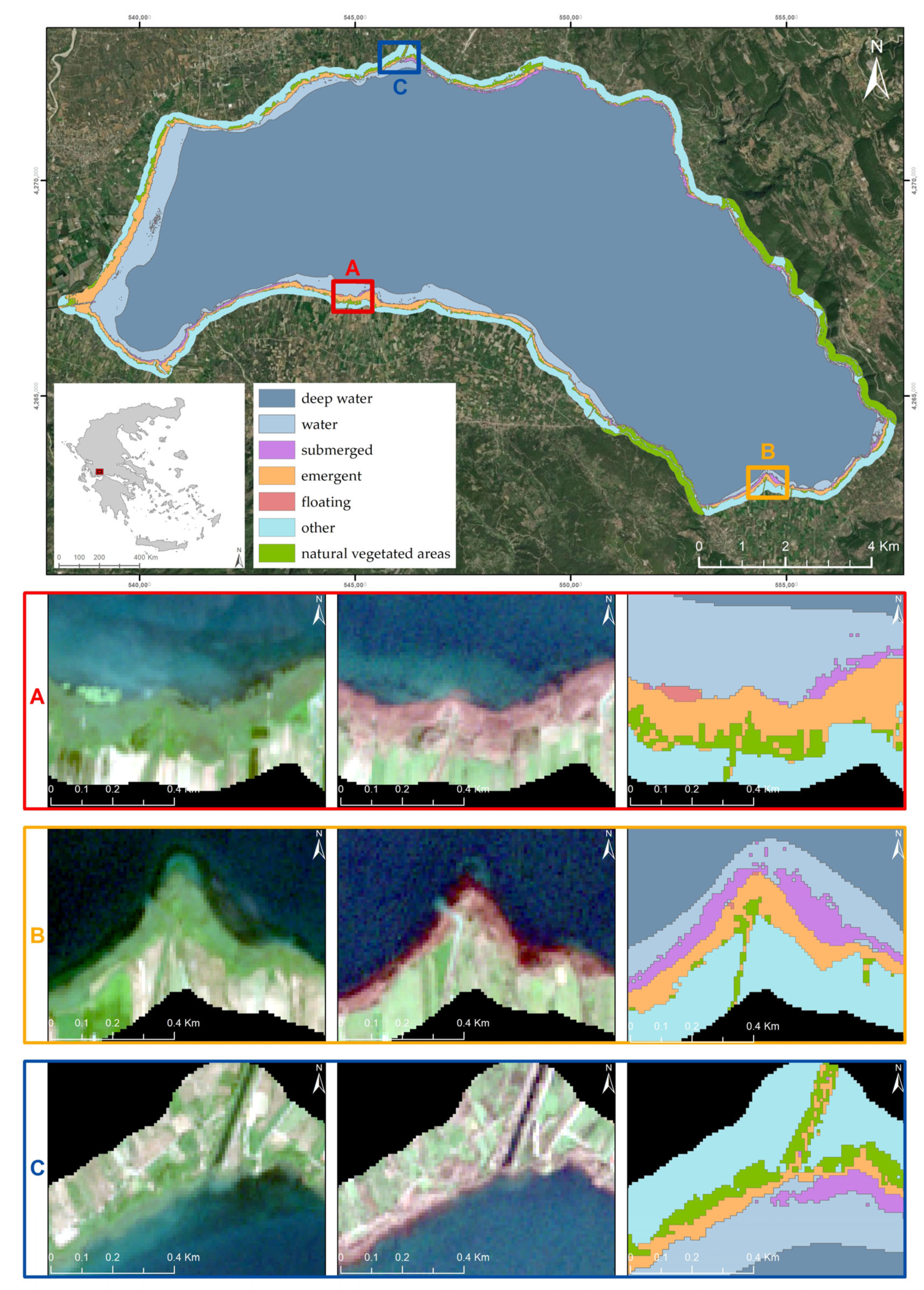
3.3. Spatial Extent per Class

The classification results of both study areas, in terms of spatial extent (in hectares) of each class and their respective percentages, are shown in

Table 7. Total spatial extents (ha) and the respective percentages of all classes in study areas, as they resulted from the classification process.

	Trichonida Lake		Feneos Lake
	Spatial Extent (ha)	%	Spatial Extent (ha)	%
Water	638	6.08	9.67	7.53
Deep Water	8545	81.42	32.58	25.38
Other	673	6.42	11.01	8.58
Natural vegetated areas	263	2.51	71.13	55.41
Emergent	285	2.72	3.10	2.42
Floating	1	0.01	-	-
Submerged	89	0.85	0.89	0.69
Total (ha)	10,495		128.38

. In Trichonida Lake, FAV covers the smallest area (1 ha or 0.01% of the total area) which confirms that although this particular type of cover is very limited, we were able to identify it based on its spectral differentiation. Similarly, SAV covers a small area; in Trichonida Lake, it covers 89 ha or 0.85% of the total extent, and in Feneos Lake, 0.89 ha or 0.69% of the total extent.

4. Discussion

Our results support that the proposed workflow, comprising a geographic object-based image approach based on spectral indices, was suitable for mapping aquatic vegetation, particularly in oligotrophic/mesotrophic deep lakes. The hierarchical object-based classification model proved to be effective in discriminating the classes of interest (EAV, FAV, SAV) in both study areas. In Trichonida Lake, where the classification model was developed, the high overall accuracy (OA = 89.31%, KIA = 0.8716) demonstrates that GEOBIA can provide a framework that can be used to integrate data of more complex environments such as aquatic ones. The high overall accuracy (OA = 89.12%, KIA = 0.8613) achieved in Feneos Lake, where the model was applied, indicates that the model can be transferred to other study areas with the same characteristics. Figure 4 and Figure 5 show examples of classification results in both lakes. It is important to note that in order to give an unbiased assessment of our mapping approach performance, the training samples used within the CART algorithm differed from the in situ data. This was decided because there were a limited number of plots for Trichonida Lake, with >80% covered by one vegetation type and with a sporadic spatial allocation (only 64), where we could apply per-plot-based splitting between training and validation subsets; thus, we opted to reserve them for the accuracy assessment [49].

Moreover, our study shows that in order to identify all vegetated classes, the incorporation of seasonal spectral information is important, since such a combination facilitates their segregation, a result also demonstrated in other studies [34,39,40]. Specifically, both producer’s accuracy (PA) and user’s accuracy (UA) scores of all vegetation classes (i.e., Emergent, Floating, Submerged, Natural vegetated areas), confirm the importance of seasonal spectral information in their classification. Moreover, the efficacy of spectral indices to discern vegetated classes is high, indicating their usefulness as a support tool in aquatic vegetation monitoring. Combinations of spectral indices, due to their flexibility, easy implementation, and high efficiency, have been widely applied in remote sensing for distinguishing different types of aquatic vegetation [48,49,101,102,103]. The classification of EAV and FAV classes result in more accurate outcomes compared to SAV, as expected; this is a common result among approaches with similar objectives [30,49,104]. This was achieved mainly because the relevant objects differed in their spectral response due to both water permanency throughout most of the year and to their phenological seasonal differences [105]. The best-performing aquatic vegetation type of our model is EAV (Table 5); the multi-temporal spectral indices NDWI ((ws) − (ss)) and mono-temporal NDRE (ss) result in high PA and UA scores in both study areas. FAV was present only in Trichonida Lake, with small but dense patches that were classified with high accuracy. The UA and PA scores of this particular class indicate a slight over-classification result from WAVI ((ss) − (ws)) and NDAVI ((ws) − (ss)) values, which occurred due to spatial resolution limitations. More specifically, there were cases of (a) pixel-sized objects with FAV covering smaller-than-pixel-sized areas and (b) pixel-sized objects mixed with FAV and EAV with greater coverage of FAV in comparison to EAV. In both cases, these areas were classified as FAV. These over-classifications were minor and thus accepted; the alternative option led to the under-estimation of FAV abundance, as the areas covered by FAV patches in Trichonida Lake are small. It should be noted that no further classification rules were required for the discrimination of potential algal blooms (AB) from FAV, as would be in the case in eutrophic lakes [106], since such phenomena were absent in both lakes. Despite the need to monitor SAV, since it has been recognized as a key component of lake ecosystems and an indicator of their ecological status, this task remains a difficult one, particularly at large spatial scales. Although the recent progress in remote sensing of SAV is significant, its monitoring is still mainly undertaken by field surveys [107]. SAV exhibits significant alterations in terms of spectral identity, spatial distribution, abundance, depth of occurrence, species variety, etc. [28]. Similar studies have reported low SAV accuracies as well [30,49,104]. We set a classification rule that effectively detects objects of submerged vegetation, even though there are cases of under-classification related mainly to the spectral variation of SAV communities’ composition and to the impact of water depth in deep lakes with high water transparency and thus a high maximum depth of macrophyte colonization [28].

Our results indicate that patches of SAV communities dominated by the aquatic angiosperm Vallisneria spiralis were systematically classified as SAV in this analysis, most probably because of their spectral characteristics [108,109,110]. Based on bathymetric data, we observed that the accuracy of the classification was higher with increased V. spiralis abundance in water depths up to 5 m. In deeper areas (~5 m<), although we observed under-classification, in terms of spatial distribution, the model managed to consistently detect patches of V. spiralis. The monitoring of V. spiralis is crucial, among other reasons, because it is being used as an ecological engineering species for aquatic ecosystem restoration based on its ability to remove excess nutrients from the water body [109]. However, areas of SAV with communities dominated by other species such as Myriophyllum spicatum, Najas marina, and Potamogeton lucens in the case of Trichonida Lake and communities dominated by M. spicatum and species of the Characeae family in the case of Feneos Lake were not classified as SAV with the same accuracy. These particular communities were present in both shallow and deep parts of the lakes. It has been observed that in the shallow parts (~up to 3 m), the model was able to detect these particular communities, while in the deeper parts (~3 m-C_max), there was minimum detection. This is probably a result of their spectral characteristics (leading to weaker spectral signal), the population density, or the species’ depth distribution (Figure 6).

We tried to find an optimal classification rule that would be able to discriminate these particular SAV communities or SAV patches with mixed species bodies. However, all efforts concluded in the significant over-classification of SAV, an outcome which was inadmissible. PA and UA scores of the classes “Water” and SAV in both study areas show that our initial goal—that any over-classification of SAV is unwanted—was attained. In addition, SAV located in deeper parts (>10 m) of the water extent cannot be sufficiently classified, as these scores indicate. Τhis applies also in the cases of either sparse submerged vegetation plots or mixed-species plots, which presented multiple differences in their spectral response within parts of the same lake. The contribution of very-high-resolution (VHR) data or UAV–acquired data would be a worthwhile endeavor in this matter [111,112]. However, such approach was beyond the scope of our study.

The final rule, which is based on seasonal spectral differentiations of NDAVI ((ws)-(ss)) values combined with mean blue (ss) values, ended in a satisfactory overall classification result of SAV with the highest possible accuracy. This was based mainly on (a) the distribution of dense patches of V. spiralis, which exhibit strong spectral identity, and (b) the spatial detection of certain under-classified SAV communities. Thus, our approach provides a useful tool for the design of aquatic vegetation monitoring.

Remote sensing is competent tool to complement and extend in situ measurements, providing frequent observations both for near-real-time and retrospective analyses [37]. In this context, our methodology can form a baseline for frequent observations of the spatial distribution of the classes of interest and the changes in their abundance. At the same time, it seems to be a valuable tool for the detection of SAV communities in the deeper parts of lakes. Furthermore, it can be applied in lakes under monitoring prior to field surveys to enable the in situ evaluation of certain areas that are not within established transects. Finally, it can be tested in lakes that are not yet included in the Monitoring Network as a means to determine the appropriate survey areas.

5. Conclusions

In this study, we have developed a hierarchical geographic object-based image classification model with multi-seasonal Sentinel-2 imagery and suitable spectral indices for large-scale aquatic vegetation mapping. Our findings show the effectiveness of utilizing Sentinel-2 imagery, especially when incorporating multi-seasonal information. Furthermore, spectral indices have been evaluated as sufficient for discriminating different aquatic vegetation classes, leading to a more robust and simpler model. Although we encountered challenges in classifying certain vegetation patches (i.e., SAV communities), our approach provides a flexible methodology for aquatic vegetation mapping and can complement in situ methods for monitoring design and implementation. We aim to test and assess this approach in other Mediterranean lakes, foreseeing necessary adjustments, to enhance its applicability for monitoring purposes.

References

1. Collen, B.; Whitton, F.; Dyer, E.E.; Baillie, J.E.M.; Cumberlidge, N.; Darwall, W.R.T.; Pollock, C.; Richman, N.I.; Soulsby, A.-M.; Böhm, M. Global patterns of freshwater species diversity, threat and endemism. Glob. Ecol. Biogeogr. 2014, 23, 40–51. [Google Scholar] [CrossRef]
2. Garcia-Moreno, J.; Harrison, I.J.; Dudgeon, D.; Clausnitzer, V.; Darwall, W.; Farrell, T.; Savy, C.; Tockner, K.; Tubbs, N. Sustaining Freshwater Biodiversity in the Anthropocene. In The Global Water System in the Anthropocene: Challenges for Science and Governance; Bhaduri, A., Bogardi, J., Leentvaar, J., Marx, S., Eds.; Springer International Publishing: Cham, Switzerland, 2014; pp. 247–270. [Google Scholar]
3. Likens, G.E. Lake Ecosystem Ecology: A Global Perspective; Elsevier Science: Amsterdam, The Netherlands, 2010. [Google Scholar]
4. Ormerod, S.J.; Dobson, M.; Hildrew, A.G.; Townsend, C.R. Multiple stressors in freshwater ecosystems. Freshw. Biol. 2010, 55, 1–4. [Google Scholar] [CrossRef]
5. Almond, R.E.A.; Grooten, M.; Peterson, T. (Eds.) Living Planet Report 2020—Bending the Curve of Biodiversity Loss; World Wildlife Fund: Gland, Switzerland, 2020. [Google Scholar]
6. Revenga, C.; Campbell, I.C.; Abell, R.; Villiers, P.D.; Bryer, M. Prospects for monitoring freshwater ecosystems towards the 2010 targets. Philos. Trans. R. Soc. B Biol. Sci. 2005, 360, 397–413. [Google Scholar] [CrossRef]
7. ISO 5667-4:1987; Guidance on Sampling from Lakes, Natural and Man-Made. International Organization for Standardization: Geneva, Switzerland, 1987.
8. ISO 5667-4:2016; Guidance on Sampling from Lakes, Natural and Man-Made. International Organization for Standardization: Geneva, Switzerland, 2016.
9. ILNAS-EN 15204:2006; Water Quality—Guidance Standard on the Enumeration of Phytoplankton Using Inverted Microscopy (Utermohl Method). Institut Luxembourgeois de la Normalisation, de l’Accréditation, de la Sécurité et qualité des produits et services: Luxembourg, 2006.
10. Birk, S.; Bonne, W.; Borja, A.; Brucet, S.; Courrat, A.; Poikane, S.; Solimini, A.; van de Bund, W.; Zampoukas, N.; Hering, D. Three hundred ways to assess Europe’s surface waters: An almost complete overview of biological methods to implement the Water Framework Directive. Ecol. Indic. 2012, 18, 31–41. [Google Scholar] [CrossRef]
11. European Communities. Directive 2000/60/EC of the European Parliament and of the Council of 23 October 2000 Establishing a framework for Community Action in the Field of Water Policy. Eur. Communities 2000, L327, 1–73. [Google Scholar]
12. European Communities. Commission Decision (EU) 2018/229 of 12 February 2018 establishing, pursuant to Directive 2000/60/EC of the European Parliament and of the Council, the values of the Member State monitoring system classifications as a result of the intercalibration exercise and repealing Commission Decision 2013/480/EU. Off. J. Eur. Communities 2018, L47, 1–91. [Google Scholar]
13. Carpenter, S.R.; Lodge, D.M. Effects of submersed macrophytes on ecosystem processes. Aquat. Bot. 1986, 26, 341–370. [Google Scholar] [CrossRef]
14. Jeppesen, E.; Søndergaard, M.; Søndergaard, M.; Christoffersen, K. (Eds.) The Structuring Role of Submerged Macrophytes in Lakes; Springer: New York, NY, USA, 1998; Volume 131, pp. 381–427. [Google Scholar]
15. Barko, J.W.; Gunnison, D.; Carpenter, S.R. Sediment interactions with submersed macrophyte growth and community dynamics. Aquat. Bot. 1991, 41, 41–65. [Google Scholar] [CrossRef]
16. Gumbricht, T. Nutrient removal processes in freshwater submersed macrophyte systems. Ecol. Eng. 1993, 2, 1–30. [Google Scholar] [CrossRef]
17. Chambers, P.; Lacoul, P.; Murphy, K.; Thomaz, S. Global diversity of aquatic macrophytes in freshwater. Hydrobiologia 2008, 595, 9–26. [Google Scholar] [CrossRef]
18. Penning, W.E.; Dudley, B.; Mjelde, M.; Hellsten, S.; Hanganu, J.; Kolada, A.; van den Berg, M.; Poikane, S.; Phillips, G.; Willby, N.; et al. Using aquatic macrophyte community indices to define the ecological status of European lakes. Aquat. Ecol. 2008, 42, 253–264. [Google Scholar] [CrossRef]
19. Penning, W.E.; Mjelde, M.; Dudley, B.; Hellsten, S.; Hanganu, J.; Kolada, A.; Van Den Berg, M.; Poikane, S.; Phillips, G.; Willby, N.; et al. Classifying aquatic macrophytes as indicators of eutrophication in European lakes. Aquat. Ecol. 2008, 42, 237–251. [Google Scholar] [CrossRef]
20. Zhang, Y.; Liu, X.; Qin, B.; Shi, K.; Deng, J.; Zhou, Y. Aquatic vegetation in response to increased eutrophication and degraded light climate in Eastern Lake Taihu: Implications for lake ecological restoration. Sci. Rep. 2016, 6, 23867. [Google Scholar] [CrossRef]
21. Poikane, S.; Portielje, R.; Denys, L.; Elferts, D.; Kelly, M.; Kolada, A.; Mäemets, H.; Phillips, G.; Søndergaard, M.; Willby, N.; et al. Macrophyte assessment in European lakes: Diverse approaches but convergent views of ‘good’ecological status. Ecol. Indic. 2018, 94, 185–197. [Google Scholar] [CrossRef]
22. Phillips, G.; Willby, N.; Moss, B. Submerged macrophyte decline in shallow lakes: What have we learnt in the last forty years? Aquat. Bot. 2016, 135, 37–45. [Google Scholar] [CrossRef]
23. Zervas, D.; Tsiaoussi, V.; Tsiripidis, I. HeLM: A macrophyte-based method for monitoring and assessment of Greek lakes. Environ. Monit. Assess. 2018, 190, 326. [Google Scholar] [CrossRef]
24. Geist, J.; Hawkins, S.J. Habitat recovery and restoration in aquatic ecosystems: Current progress and future challenges. Aquat. Conserv. Mar. Freshw. Ecosyst. 2016, 26, 942–962. [Google Scholar] [CrossRef]
25. Rohal, C.; Reynolds, L.; Adams, C.; Martin, C.; Latimer, E.; Walsh, S.; Slater, J. Biological and practical tradeoffs in planting techniques for submerged aquatic vegetation. Aquat. Bot. 2021, 170, 103347. [Google Scholar] [CrossRef]
26. Carvalho, L.; Mackay, E.B.; Cardoso, A.C.; Baattrup-Pedersen, A.; Birk, S.; Blackstock, K.L.; Borics, G.; Borja, A.; Feld, C.K.; Ferreira, M.T.; et al. Protecting and restoring Europe’s waters: An analysis of the future development needs of the Water Framework Directive. Sci. Total. Environ. 2019, 658, 1228–1238. [Google Scholar] [CrossRef]
27. Free, G.; Bresciani, M.; Trodd, W.; Tierney, D.; O’Boyle, S.; Plant, C.; Deakin, J. Estimation of lake ecological quality from Sentinel-2 remote sensing imagery. Hydrobiologia 2020, 847, 1423–1438. [Google Scholar] [CrossRef]
28. Rowan, G.S.L.; Kalacska, M. A Review of Remote Sensing of Submerged Aquatic Vegetation for Non-Specialists. Remote Sens. 2021, 13, 623. [Google Scholar] [CrossRef]
29. Visser, F.; Wallis, C.; Sinnott, A.M. Optical remote sensing of submerged aquatic vegetation: Opportunities for shallow clearwater streams. Limnologica 2013, 43, 388–398. [Google Scholar] [CrossRef]
30. Silva, T.S.F.; Costa, M.P.F.; Melack, J.M.; Novo, E.M.L.M. Remote sensing of aquatic vegetation: Theory and applications. Environ. Monit. Assess. 2008, 140, 131–145. [Google Scholar] [CrossRef]
31. Dörnhöfer, K.; Oppelt, N. Remote sensing for lake research and monitoring–Recent advances. Ecol. Indic. 2016, 64, 105–122. [Google Scholar] [CrossRef]
32. Knipling, E.B. Physical and physiological basis for the reflectance of visible and near-infrared radiation from vegetation. Remote Sens. Environ. 1970, 1, 155–159. [Google Scholar] [CrossRef]
33. Liu, X.; Zhang, Y.; Shi, K.; Zhou, Y.; Tang, X.; Zhu, G.; Qin, B. Mapping Aquatic Vegetation in a Large, Shallow Eutrophic Lake: A Frequency-Based Approach Using Multiple Years of MODIS Data. Remote Sens. 2015, 7, 10295–10320. [Google Scholar] [CrossRef]
34. Luo, J.; Li, X.; Ma, R.; Li, F.; Duan, H.; Hu, W.; Qin, B.; Huang, W. Applying remote sensing techniques to monitoring seasonal and interannual changes of aquatic vegetation in Taihu Lake, China. Ecol. Indic. 2016, 60, 503–513. [Google Scholar] [CrossRef]
35. Marshall, T.R.; Lee, P. Mapping aquatic macrophytes through digital image analysis of aerial photographs: An assessment. J. Aquat. Plant Manag. 1994, 32, 61–66. [Google Scholar]
36. Pu, R.; Bell, S. Mapping seagrass coverage and spatial patterns with high spatial resolution IKONOS imagery. Int. J. Appl. Earth Obs. Geoinf. 2017, 54, 145–158. [Google Scholar] [CrossRef]
37. Villa, P.; Pinardi, M.; Tóth, V.R.; Hunter, P.D.; Bolpagni, R.; Bresciani, M. Remote sensing of macrophyte morphological traits: Implications for the management of shallow lakes. J. Limnol. 2017, 76, 109–126. [Google Scholar] [CrossRef]
38. Welch, R.; Remillard, M.; Slack, R. Remote sensing and geographic information system techniques for aquatic resource evaluation. In (American Society for Photogrammetry and Remote Sensing and ACSM, Annual Convention, Baltimore, MD, USA, 29 March–3 April 1987) Photogrammetric Engineering and Remote Sensing; American Society for Photogrammetry and Remote Sensing and ACSM: Reno, NV, USA, 1988; pp. 177–185. [Google Scholar]
39. Luo, J.; Duan, H.; Ma, R.; Jin, X.; Li, F.; Hu, W.; Shi, K.; Huang, W. Mapping species of submerged aquatic vegetation with multi-seasonal satellite images and considering life history information. Int. J. Appl. Earth Obs. Geoinf. 2017, 57, 154–165. [Google Scholar] [CrossRef]
40. Elijah, W.R., III; Laine, S.C. Comparison of Landsat Thematic Mapper and High Resolution Photography to Identify Change in Complex Coastal Wetlands. J. Coast. Res. 1997, 13, 281–292. [Google Scholar]
41. Ade, C.; Khanna, S.; Lay, M.; Ustin, S.L.; Hestir, E.L. Genus-Level Mapping of Invasive Floating Aquatic Vegetation Using Sentinel-2 Satellite Remote Sensing. Remote Sens. 2022, 14, 3013. [Google Scholar] [CrossRef]
42. Farmer, A.M.; Adams, M.S. A consideration of the problems of scale in the study of the ecology of aquatic macrophytes. Aquat. Bot. 1989, 33, 177–189. [Google Scholar] [CrossRef]
43. Vis, C.; Hudon, C.; Carignan, R. An evaluation of approaches used to determine the distribution and biomass of emergent and submerged aquatic macrophytes over large spatial scales. Aquat. Bot. 2003, 77, 187–201. [Google Scholar] [CrossRef]
44. Chen, Q.; Yu, R.; Hao, Y.; Wu, L.; Zhang, W.; Zhang, Q.; Bu, X. A New Method for Mapping Aquatic Vegetation Especially Underwater Vegetation in Lake Ulansuhai Using GF-1 Satellite Data. Remote Sens. 2018, 10, 1279. [Google Scholar] [CrossRef]
45. Davranche, A.; Lefebvre, G.; Poulin, B. Wetland monitoring using classification trees and SPOT-5 seasonal time series. Remote Sens. Environ. 2010, 114, 552–562. [Google Scholar] [CrossRef]
46. Rodríguez-Garlito, E.C.; Paz-Gallardo, A.; Plaza, A. Mapping Invasive Aquatic Plants in Sentinel-2 Images Using Convolutional Neural Networks Trained With Spectral Indices. IEEE J. Sel. Top. Appl. Earth Obs. Remote Sens. 2023, 16, 2889–2899. [Google Scholar] [CrossRef]
47. Zhao, D.; Lv, M.; Jiang, H.; Cai, Y.; Xu, D.; An, S. Spatio-Temporal Variability of Aquatic Vegetation in Taihu Lake over the Past 30 Years. PLoS ONE 2013, 8, e66365. [Google Scholar] [CrossRef]
48. Luo, J.; Ma, R.; Duan, H.; Hu, W.; Zhu, J.; Huang, W.; Lin, C. A New Method for Modifying Thresholds in the Classification of Tree Models for Mapping Aquatic Vegetation in Taihu Lake with Satellite Images. Remote Sens. 2014, 6, 7442–7462. [Google Scholar] [CrossRef]
49. Villa, P.; Bresciani, M.; Bolpagni, R.; Pinardi, M.; Giardino, C. A rule-based approach for mapping macrophyte communities using multi-temporal aquatic vegetation indices. Remote Sens. Environ. 2015, 171, 218–233. [Google Scholar] [CrossRef]
50. de Grandpré, A.; Kinnard, C.; Bertolo, A. Open-Source Analysis of Submerged Aquatic Vegetation Cover in Complex Waters Using High-Resolution Satellite Remote Sensing: An Adaptable Framework. Remote Sens. 2022, 14, 267. [Google Scholar] [CrossRef]
51. Visser, F.; Buis, K.; Verschoren, V.; Schoelynck, J. Mapping of submerged aquatic vegetation in rivers from very high-resolution image data, using object-based image analysis combined with expert knowledge. Hydrobiologia 2018, 812, 157–175. [Google Scholar] [CrossRef]
52. Chabot, D.; Dillon, C.; Shemrock, A.; Weissflog, N.; Sager, E.P.S. An Object-Based Image Analysis Workflow for Monitoring Shallow-Water Aquatic Vegetation in Multispectral Drone Imagery. ISPRS Int. J. Geo-Inf. 2018, 7, 294. [Google Scholar] [CrossRef]
53. Husson, E.; Ecke, F.; Reese, H. Comparison of Manual Mapping and Automated Object-Based Image Analysis of Non-Submerged Aquatic Vegetation from Very-High-Resolution UAS Images. Remote Sens. 2016, 8, 724. [Google Scholar] [CrossRef]
54. Hay, G.J.; Castilla, G. Geographic Object-Based Image Analysis (GEOBIA): A new name for a new discipline. In Object-Based Image Analysis: Spatial Concepts for Knowledge-Driven Remote Sensing Applications; Springer: Berlin/Heidelberg, Germany, 2008; pp. 75–89. [Google Scholar]
55. Mavromati, E.; Kagalou, I.; Kemitzoglou, D.; Apostolakis, A.; Seferlis, M.; Tsiaoussi, V. Relationships Among Land Use Patterns, Hydromorphological Features and Physicochemical Parameters of Surface Waters: WFD Lake Monitoring in Greece. Environ. Process. 2018, 5, 139–151. [Google Scholar] [CrossRef]
56. Apostolakis, A.P.D.; Demertzi, K. Isobaths of Lake Trichonida. Greek Biotope Wetland Centre EKBY. 2021. Available online: http://ekbygis.biodiversity-info.gr/geonetwork/srv/eng/main.home (accessed on 15 September 2022).
57. Kottek, M.; Grieser, J.; Beck, C.; Rudolf, B.; Rubel, F. World map of the Köppen-Geiger climate classification updated. Meteorol. Zeitschrif 2006, 15, 259–263. [Google Scholar] [CrossRef]
58. Kagalou, I.; Ntislidou, C.; Latinopoulos, D.; Kemitzoglou, D.; Tsiaoussi, V.; Bobori, D.C. Setting the Phosphorus Boundaries for Greek Natural Shallow and Deep Lakes for Water Framework Directive Compliance. Water 2021, 13, 739. [Google Scholar] [CrossRef]
59. Gourgouletis, N.; Baltas, E. Investigating Hydroclimatic Variables Trends on the Natural Lakes of Western Greece Using Earth Observation Data. Sensors 2023, 23, 2056. [Google Scholar] [CrossRef]
60. Dimitriou, E.; Zacharias, I. Quantifying the rainfall-water level fluctuation process in a geologically complex lake catchment. Environ. Monit. Assess. 2006, 119, 491–506. [Google Scholar]
61. Seguin, J.; Avramidis, P.; Dörfler, W.; Emmanouilidis, A.; Unkel, I. A 2600-year high-resolution climate record from Lake Trichonida (SW Greece). EG Quat. Sci. J. 2020, 69, 139–160. [Google Scholar] [CrossRef]
62. Albrecht, C.; Hauffe, T.; Schreiber, K.; Trajanovski, S.; Wilke, T. Mollusc biodiversity and endemism in the potential ancient lake Trichonis, Greece. Malacologia 2009, 51, 357–375. [Google Scholar] [CrossRef]
63. Doulka, E.; Kehayias, G. Spatial and temporal distribution of zooplankton in Lake Trichonis (Greece). J. Nat. Hist. 2008, 42, 575–595. [Google Scholar] [CrossRef]
64. Obolewski, K.; SkorbiŁowicz, E.; SkorbiŁowicz, M.; Glińska-Lewczuk, K.; Astel, A.M.; Strzelczak, A. The effect of metals accumulated in reed (Phragmites australis) on the structure of periphyton. Ecotoxicol. Environ. Saf. 2011, 74, 558–568. [Google Scholar] [CrossRef]
65. Petriki, O.; Moutopoulos, D.K.; Tsagarakis, K.; Tsionki, I.; Papantoniou, G.; Mantzouni, I.; Barbieri, R.; Stoumboudi, M.T. Assessing the Fisheries and Ecosystem Structure of the Largest Greek Lake (Lake Trichonis). Water 2021, 13, 3329. [Google Scholar] [CrossRef]
66. Zervas, D.; Tsiripidis, I.; Bergmeier, E.; Tsiaousi, V. A phytosociological survey of aquatic vegetation in the main freshwater lakes of Greece. Veg. Classif. Surv. 2020, 1, 53–75. [Google Scholar] [CrossRef]
67. European Environment Agency: NATURA 2000—Standard Data Form: Limnes Trichonida Kai Lysimacheia, C., Denmark. Available online: https://natura2000.eea.europa.eu/Natura2000/SDF.aspx?site=GR2310009&release=10#7 (accessed on 1 February 2023).
68. Koussouris, T. Plankton observations in three lakes of Western Greece. Thalassographica 1978, 2, 115–123. [Google Scholar]
69. Overbeck, J.; Anagnostidis, K.; Economou-Amilli, A. Limnological Survey of Three Greek Lakes: Trichonis, Lyssimachia and Amvrakia(Ein Limnologischer Uberblick von drei Griechischen Seen: Trichonis, Lyssimachia und Amvrakia). Arch. Fur Hydrobiol. Vol. 1982, 95, 365–394. [Google Scholar]
70. Koumpli-Sovantzi, L. The Aquatic Flora of Aetoloakarnania (W Greece). Willdenowia 1989, 18, 377–385. [Google Scholar]
71. Palmer, M.; Bell, S.; Butterfield, I. A botanical classification of standing waters in Britain: Applications for conservation and monitoring. Aquat. Conserv. Mar. Freshw. Ecosyst. 1992, 2, 125–143. [Google Scholar] [CrossRef]
72. EN 15460:2007; Water Quality—Guidance Standard for the Surveying of Aquatic Macrophytes in Lakes. European Committee for Standardization: Bruxelles, Belgium, 2007.
73. EKBY. GeoServer. Available online: http://ekbygis.biodiversity-info.gr/geoserver/web/ (accessed on 15 November 2022).
74. Hutchinson, M. A locally adaptive approach to the interpolation of digital elevation models. In Proceedings of the Third International Conference/Workshop on Integrating GIS and Environmental Modeling, Sante Fe, NM, USA, 21–25 January 1996; pp. 21–26. [Google Scholar]
75. Hutchinson, M.; Xu, T.; Stein, J. Recent Progress in the ANUDEM Elevation Gridding Procedure. Geomorphometry 2011, 2011, 19–22. [Google Scholar]
76. Hutchinson, M.F. Calculation of hydrologically sound digital elevation models. In Proceedings of the Third International Symposium on Spatial Data Handling, Sydney, Australia, 17–19 August 1988; pp. 117–133. [Google Scholar]
77. Hutchinson, M.F. A new procedure for gridding elevation and stream line data with automatic removal of spurious pits. J. Hydrol. 1989, 106, 211–232. [Google Scholar] [CrossRef]
78. Hutchinson, M. Optimising the degree of data smoothing for locally adaptive finite element bivariate smoothing splines. ANZIAM J. 2000, 42, C774–C796. [Google Scholar] [CrossRef]
79. Ecosystem, C.D.S. Available online: https://dataspace.copernicus.eu/ (accessed on 15 November 2022).
80. Drusch, M.; Del Bello, U.; Carlier, S.; Colin, O.; Fernandez, V.; Gascon, F.; Hoersch, B.; Isola, C.; Laberinti, P.; Martimort, P.; et al. Sentinel-2: ESA’s Optical High-Resolution Mission for GMES Operational Services. Remote Sens. Environ. 2012, 120, 25–36. [Google Scholar] [CrossRef]
81. Warren, M.A.; Simis, S.G.H.; Martinez-Vicente, V.; Poser, K.; Bresciani, M.; Alikas, K.; Spyrakos, E.; Giardino, C.; Ansper, A. Assessment of atmospheric correction algorithms for the Sentinel-2A MultiSpectral Imager over coastal and inland waters. Remote Sens. Environ. 2019, 225, 267–289. [Google Scholar] [CrossRef]
82. Toming, K.; Kutser, T.; Laas, A.; Sepp, M.; Paavel, B.; Nõges, T. First Experiences in Mapping Lake Water Quality Parameters with Sentinel-2 MSI Imagery. Remote Sens. 2016, 8, 640. [Google Scholar] [CrossRef]
83. Kuhwald, K.; Schneider von Deimling, J.; Schubert, P.; Oppelt, N. How can Sentinel-2 contribute to seagrass mapping in shallow, turbid Baltic Sea waters? Remote Sens. Ecol. Conserv. 2022, 8, 328–346. [Google Scholar] [CrossRef]
84. Mederos-Barrera, A.; Marcello, J.; Eugenio, F.; Hernández, E. Seagrass mapping using high resolution multispectral satellite imagery: A comparison of water column correction models. Int. J. Appl. Earth Obs. Geoinf. 2022, 113, 102990. [Google Scholar] [CrossRef]
85. Fornes, A.; Basterretxea, G.; Orfila, A.; Jordi, A.; Alvarez, A.; Tintore, J. Mapping Posidonia oceanica from IKONOS. ISPRS J. Photogramm. Remote Sens. 2006, 60, 315–322. [Google Scholar] [CrossRef]
86. Phinn, S.; Roelfsema, C.; Dekker, A.; Brando, V.; Anstee, J. Mapping seagrass species, cover and biomass in shallow waters: An assessment of satellite multi-spectral and airborne hyper-spectral imaging systems in Moreton Bay (Australia). Remote Sens. Environ. 2008, 112, 3413–3425. [Google Scholar] [CrossRef]
87. Topouzelis, K.; Charalampis Spondylidis, S.; Papakonstantinou, A.; Soulakellis, N. The use of Sentinel-2 imagery for seagrass mapping: Kalloni Gulf (Lesvos Island, Greece) case study. In Proceedings of the Fourth International Conference on Remote Sensing and Geoinformation of the Environment, Pafos, Cyprus, 4–8 April 2016; SPIE: Bellingham, WA, USA, 2016; Volume 9688, pp. 460–466. [Google Scholar]
88. QGIS.org. QGIS Geographic Information System. QGIS Association. Available online: https://qgis.org/en/site/ (accessed on 15 November 2022).
89. Castilla, G.; Hay, G.J. Image objects and geographic objects. In Object-Based Image Analysis: Spatial Concepts for Knowledge-Driven Remote Sensing Applications; Blaschke, T., Lang, S., Hay, G.J., Eds.; Springer: Berlin/Heidelberg, Germany, 2008; pp. 91–110. [Google Scholar]
90. Smith, A. Image segmentation scale parameter optimization and land cover classification using the Random Forest algorithm. J. Spat. Sci. 2010, 55, 69–79. [Google Scholar] [CrossRef]
91. Townshend, J.R.G.; Justice, C.O. Analysis of the dynamics of African vegetation using the normalized difference vegetation index. Int. J. Remote Sens. 1986, 7, 1435–1445. [Google Scholar] [CrossRef]
92. Huete, A.R. A soil-adjusted vegetation index (SAVI). Remote Sens. Environ. 1988, 25, 295–309. [Google Scholar] [CrossRef]
93. McFeeters, S.K. The use of the Normalized Difference Water Index (NDWI) in the delineation of open water features. Int. J. Remote Sens. 1996, 17, 1425–1432. [Google Scholar] [CrossRef]
94. Barnes, E.M.; Clarke, T.R.; Richards, S.E.; Colaizzi, P.D.; Haberland, J.; Kostrzewski, M.; Waller, P.; Choi, C.; Riley, E.; Thompson, T.; et al. Coincident detection of crop water stress, nitrogen status and canopy density using ground-based multispectral data. In Proceedings of the Fifth International Conference on Precision Agriculture, Bloomington, MN, USA, 16–19 July 2000; pp. 1–15. [Google Scholar]
95. Villa, P.; Bresciani, M.; Braga, F.; Bolpagni, R. Comparative Assessment of Broadband Vegetation Indices Over Aquatic Vegetation. IEEE J. Sel. Top. Appl. Earth Obs. Remote Sens. 2014, 7, 3117–3127. [Google Scholar] [CrossRef]
96. Blaschke, T.; Feizizadeh, B.; Hölbling, D. Object-based image analysis and digital terrain analysis for locating landslides in the Urmia Lake Basin, Iran. IEEE J. Sel. Top. Appl. Earth Obs. Remote Sens. 2014, 7, 4806–4817. [Google Scholar] [CrossRef]
97. Breiman, L.; Friedman, J.; Ohlsen, R.; Stone, C. Classification and Regression Trees; Wadsworth International Group: Franklin, TN, USA, 1984. [Google Scholar]
98. Congalton, R.; Green, K. Assessing the Accuracy of Remotely Sensed Data: Princples and Practices; CRC Press: Boca Raton, FL, USA, 2009; pp. 1–200. [Google Scholar]
99. Tortora, R.D. A Note on Sample Size Estimation for Multinomial Populations. Am. Stat. 1978, 32, 100–102. [Google Scholar] [CrossRef]
100. Hay, A.M. The derivation of global estimates from a confusion matrix. Int. J. Remote Sens. 1988, 9, 1395–1398. [Google Scholar] [CrossRef]
101. Qing, S.; Runa, A.; Shun, B.; Zhao, W.; Bao, Y.; Hao, Y. Distinguishing and mapping of aquatic vegetations and yellow algae bloom with Landsat satellite data in a complex shallow Lake, China during 1986–2018. Ecol. Indic. 2020, 112, 106073. [Google Scholar] [CrossRef]
102. Chauhan, K.; Patel, J.; Shukla, S.H.; Kalubarme, M.H. Monitoring Water Spread and Aquatic Vegetation using Spectral Indices in Nalsarovar, Gujarat State-India. Int. J. Environ. Geoinform. 2021, 8, 49–56. [Google Scholar] [CrossRef]
103. Jaskuła, J.; Sojka, M. Assessing Spectral Indices for Detecting Vegetative Overgrowth of Reservoirs. Pol. J. Environ. Stud. 2019, 28, 4199–4211. [Google Scholar] [CrossRef]
104. Klemas, V. Remote sensing of emergent and submerged wetlands: An overview. Int. J. Remote Sens. 2013, 34, 6286–6320. [Google Scholar] [CrossRef]
105. Fitoka, E.; Tompoulidou, M.; Hatziiordanou, L.; Apostolakis, A.; Höfer, R.; Weise, K.; Ververis, C. Water-related ecosystems’ mapping and assessment based on remote sensing techniques and geospatial analysis: The SWOS national service case of the Greek Ramsar sites and their catchments. Remote Sens. Environ. 2020, 245, 111795. [Google Scholar] [CrossRef]
106. Luo, J.; Ni, G.; Zhang, Y.; Wang, K.; Shen, M.; Cao, Z.; Qi, T.; Xiao, Q.; Qiu, Y.; Cai, Y.; et al. A new technique for quantifying algal bloom, floating/emergent and submerged vegetation in eutrophic shallow lakes using Landsat imagery. Remote Sens. Environ. 2023, 287, 113480. [Google Scholar] [CrossRef]
107. Madsen, J.D.; Wersal, R.M. A review of aquatic plant monitoring and assessment methods. J. Aquat. Plant Manag. 2017, 55, 1–12. [Google Scholar]
108. Cheng, Q.; Wu, K.; Bai, Y.; Hu, Y. Research on the relationship between the fractional coverage of the submerged plant Vallisneria spiralis and observed spectral parameters. Environ. Monit. Assess. 2013, 185, 5401–5409. [Google Scholar] [CrossRef]
109. Yuan, L.; Zhang, L. Identification of the spectral characteristics of submerged plant Vallisneria spiralis. Acta Ecol. Sin. 2006, 26, 1005–1010. [Google Scholar] [CrossRef]
110. Yuan, L.; Zhang, L.-Q. The spectral responses of a submerged plant Vallisneria spiralis with varying biomass using spectroradiometer. Hydrobiologia 2007, 579, 291–299. [Google Scholar] [CrossRef]
111. Alagialoglou, L.; Manakos, I.; Papadopoulou, S.; Chadoulis, R.-T.; Kita, A. Mapping Underwater Aquatic Vegetation Using Foundation Models With Air-and Space-Borne Images: The Case of Polyphytos Lake. Remote Sens. 2023, 15, 4001. [Google Scholar] [CrossRef]
112. Lu, L.; Luo, J.; Xin, Y.; Xu, Y.; Sun, Z.; Duan, H.; Xiao, Q.; Qiu, Y.; Huang, L.; Zhao, J. A novel strategy for estimating biomass of submerged aquatic vegetation in lake integrating UAV and Sentinel data. Sci. Total. Environ. 2024, 912, 169404. [Google Scholar] [CrossRef]
Figure 1. Study areas of Trichonida Lake (a) and Feneos Lake (b) examined in this analysis. The red polygon boundary denotes the 200 m buffer zone around the respective shoreline that was determined by the mean water level (16 m above the mean sea level for Trichonida Lake and 872 m above the mean sea level for Feneos Lake). The buffer indicates the zone based on a 200 m distance from the shoreline, and it comprised the final area under investigation. Blue points denote the transects established for the in situ monitoring of aquatic vegetation for WFD purposes. The green points denote the additional plots where extra field vegetation recordings were available for Feneos Lake. These points comprise the final set of in situ recorded points used in the accuracy assessment. We used the World Topographic Map as a basemap, available in ESRI ArcGIS software v. 10.8.2.
Remotesensing 16 00916 g001
Figure 2. Hierarchical classification flow with three levels of segmentation. The links between the classes denote the relationship between them.
Remotesensing 16 00916 g002
Figure 3. The classification ruleset as it was developed in the study area of Trichonida Lake. Features derived from winter season and summer season images are denoted with (ws) and (ss), respectively. Prior to its application in the second study area of Feneos Lake, the ruleset was evaluated for its performance and minor adjustments were made to the respective range of values of the features.
Remotesensing 16 00916 g003
Figure 4. Examples of classification results in Trichonida Lake. The first two columns indicate the Sentinel 2A images for summer and winter season, respectively; the third column shows the classification result. In case (A), patches of floating vegetation (pink) can be observed in the image of summer season, while in all cases the emergent vegetation (orange) demonstrates a characteristic spectral differentiation between seasons. In cases (B,C), pictures show the distribution of submerged vegetation (purple) as it resulted from NDAVI ((ws) − (ss)) values combined with mean blue (ss) values.
Remotesensing 16 00916 g004
Figure 5. Examples of classification results in Feneos Lake. The first two columns indicate the Sentinel 2A images for summer and winter season, respectively; the third column shows the classification result. In cases (A,B), we observe the high discrimination of the emergent aquatic vegetation class, while the submerged aquatic vegetation was slightly less accurate. In case (C), the submerged aquatic vegetation class in the shallow part of the lake was very well discriminated, although this does not apply for the deeper part (almost near the “Deep Water” class (dark blue) where we observed, during our survey, patches of Vallisneria spiralis).
Remotesensing 16 00916 g005
Figure 6. Examples of the classified objects for the “Submerged” class (purple). The polygons with yellow color—produced through digitization solely for demonstration purposes—define areas covered by submerged aquatic vegetation (based on in situ data and expert photointerpretation). It can be observed that, in cases (c,d,f), the submerged communities dominated by Myriophyllum spicatum, Najas marina, and Potamogeton lucens, particularly in the deeper parts of the lake, were under-classified. This is mainly due to the differences in spectral characteristics of the particular communities in different depths. Several tests for their discrimination led to unwanted over-classifications. In the other cases (a,b,e,gi), it can be observed that the submerged communities dominated by the Vallisneria spiralis have been systematically classified.
Remotesensing 16 00916 g006