
ASPP+-LANet: A Multi-Scale Context Extraction Network for Semantic Segmentation of High-Resolution Remote Sensing Images


Abstract
1. Introduction
- (1)
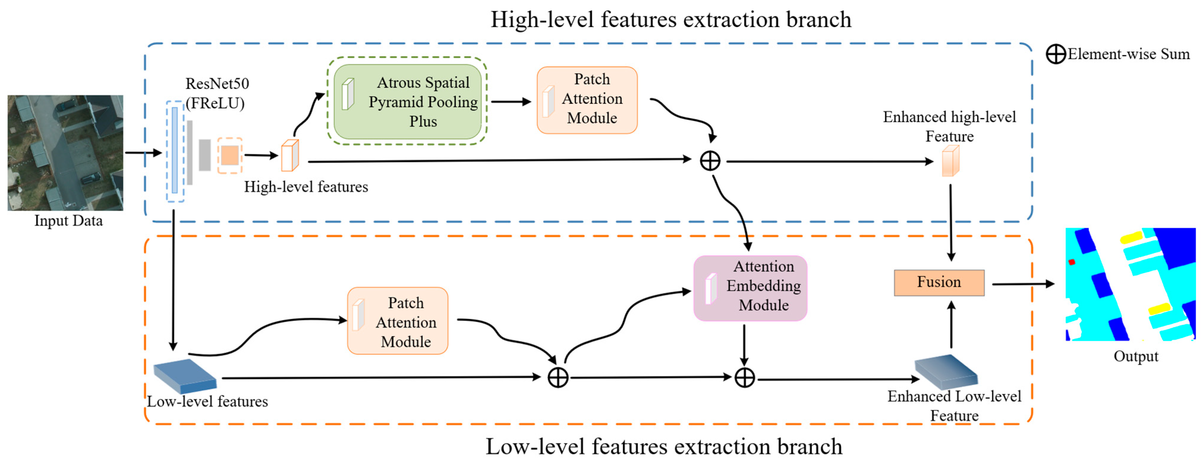
- We propose a multi-scale context extraction network for semantic segmentation of high-resolution RS images, ASPP+-LANet, by improving the LANet structure, which effectively tackles the issue of unclear segmentation in various-sized ground objects, slender ground objects, and ground object edges. By adding a new multi-scale module, the segmentation accuracy of ground objects at different scales has been improved. By introducing the activation function, the segmentation accuracy of slender ground objects and ground object edges has been improved.
- (2)
- We designed a novel ASPP+ module to effectively enhance the segmentation accuracy of ground objects at different sizes. This module adds an additional feature extraction channel to ASPP. In addition, we redesigned its dilation rates and introduced the CA mechanism. The attention mechanism can focus on more meaningful areas, improving the overall segmentation progress.
- (3)
- We introduced the FReLU activation function. By integrating it with the LANet network, the performance of ASPP+-LANet has been improved. The activation function can filter out noise and low-frequency information and retain more higher-frequency information so as to effectively enhance the segmentation accuracy of slender ground objects and ground object edges.
2. Materials and Methods
2.1. Materials
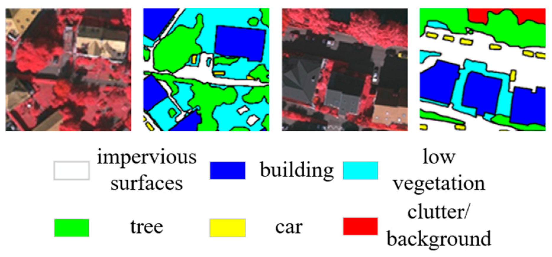
2.1.1. Potsdam Datasets
2.1.2. Vaihingen Datasets
2.2. Methods
2.2.1. Overall Network Structure
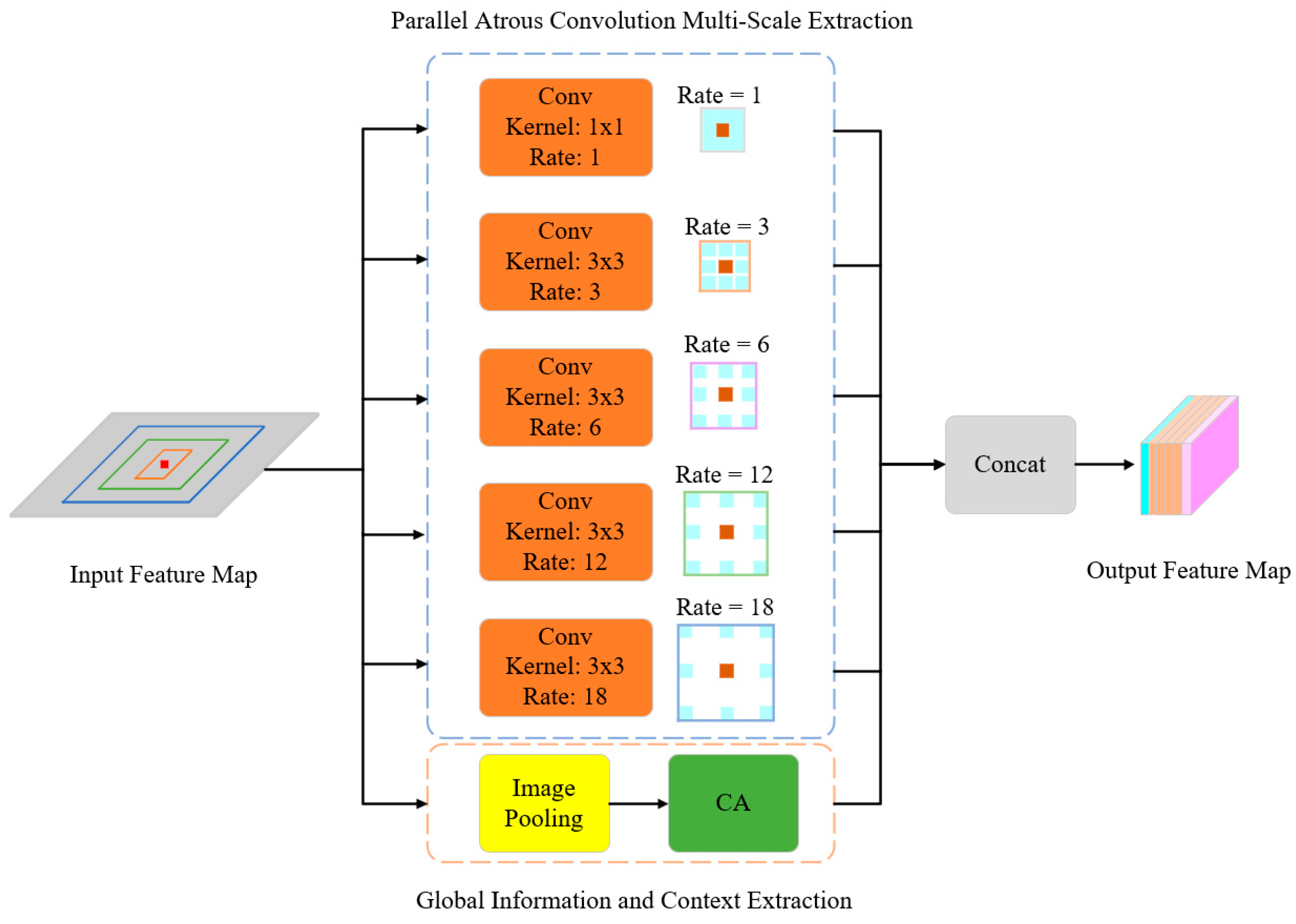
2.2.2. ASPP+ Module
- (1)
- Parallel Dilated Convolution Multi-Scale Feature Extraction
- (a)
- The combination of dilation rates should not have a common factor greater than 1, as it would still lead to the occurrence of the “grid effect”.
- (b)
- Assuming that dilation rates corresponding to N convolutional kernel sizes of atrous convolutions are , it is required that Equation (1) satisfies .where represents the dilation rate of the i-th atrous convolution and represents the maximum dilation rate for the i-th layer of atrous convolution, with a default value of .
- (2)
- Global features and contextual information extraction
2.2.3. FReLU
3. Experiments and Results
3.1. Evaluation Criteria
3.2. Implementation Details
3.3. Experiment Results
3.3.1. Segmentation Precision Analysis
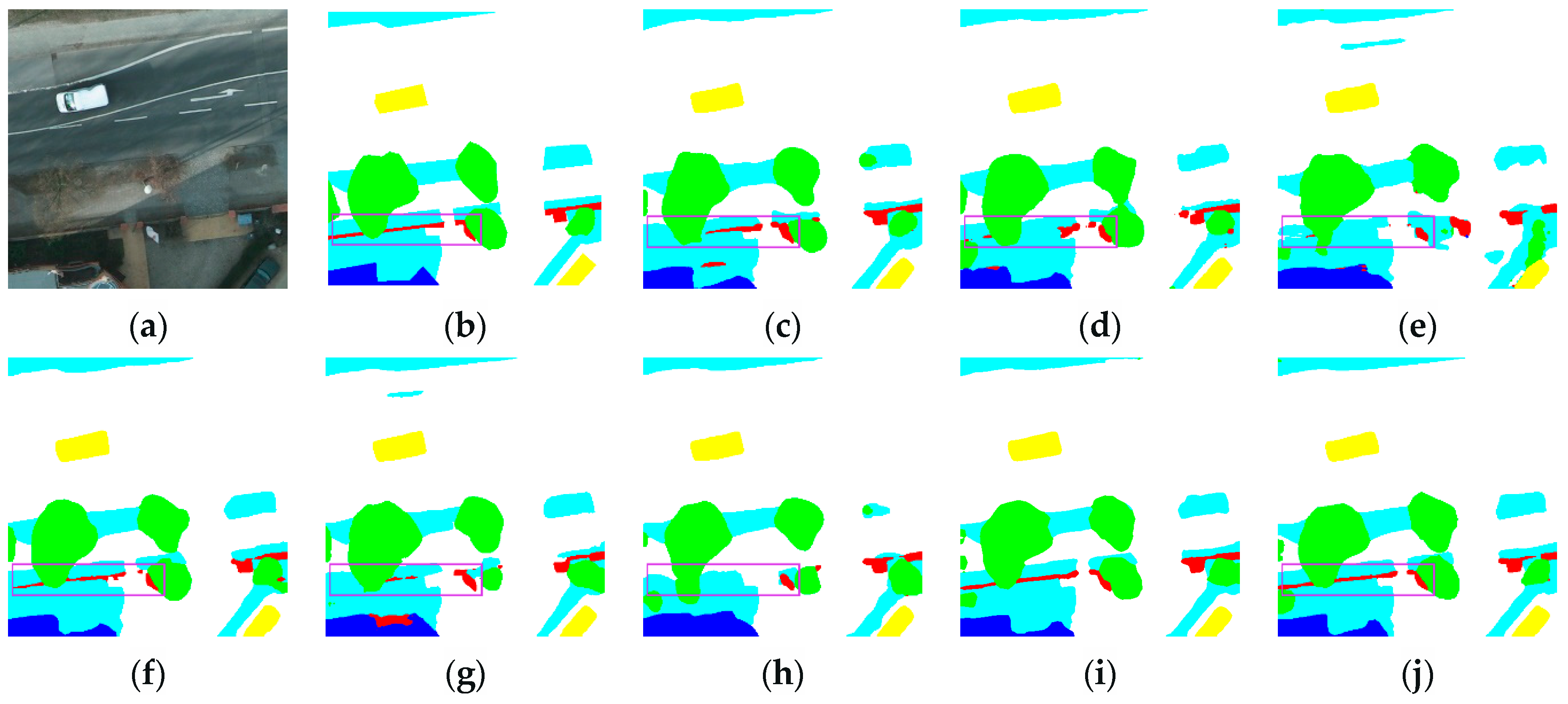
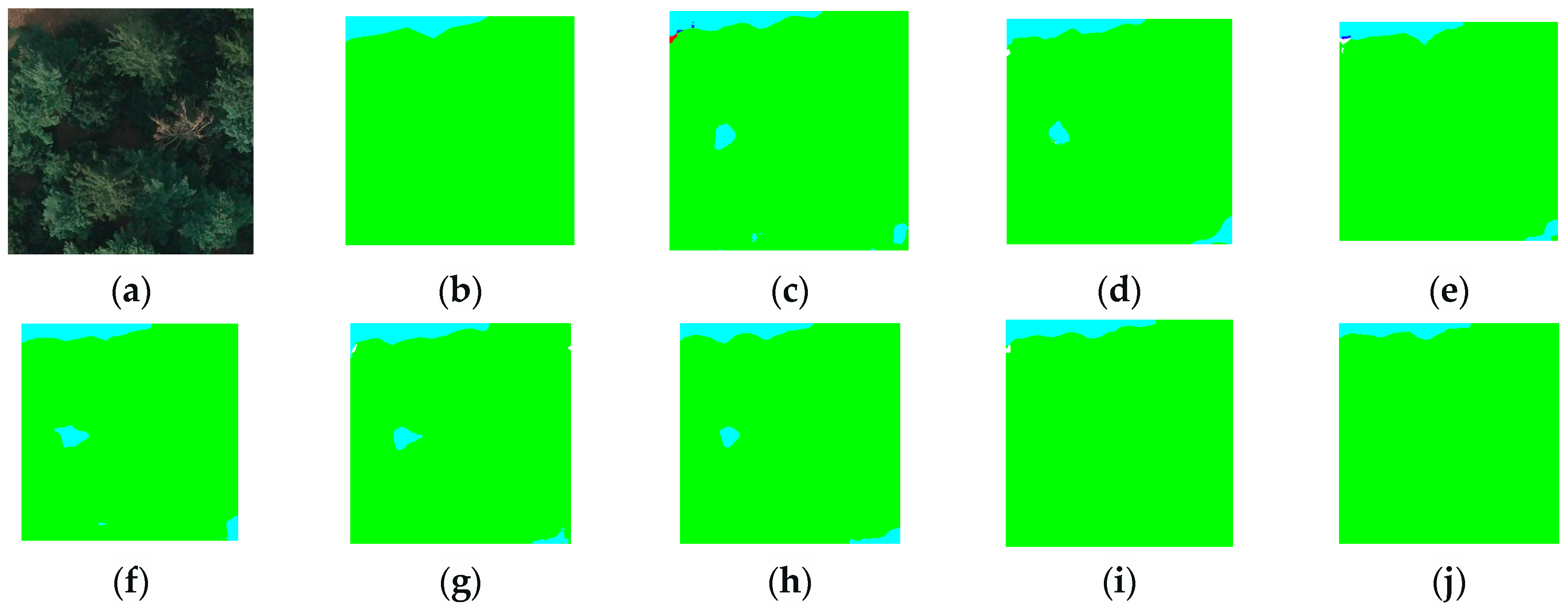
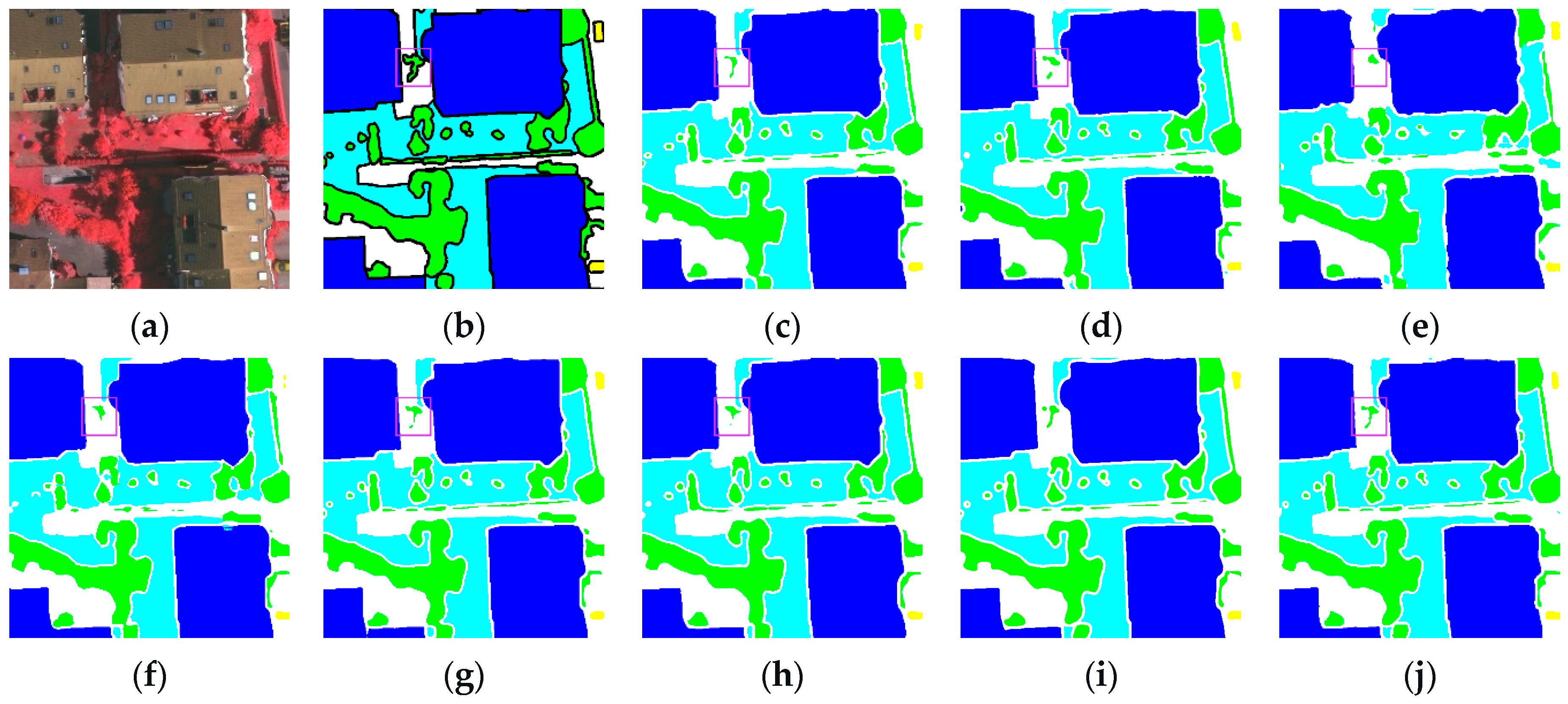
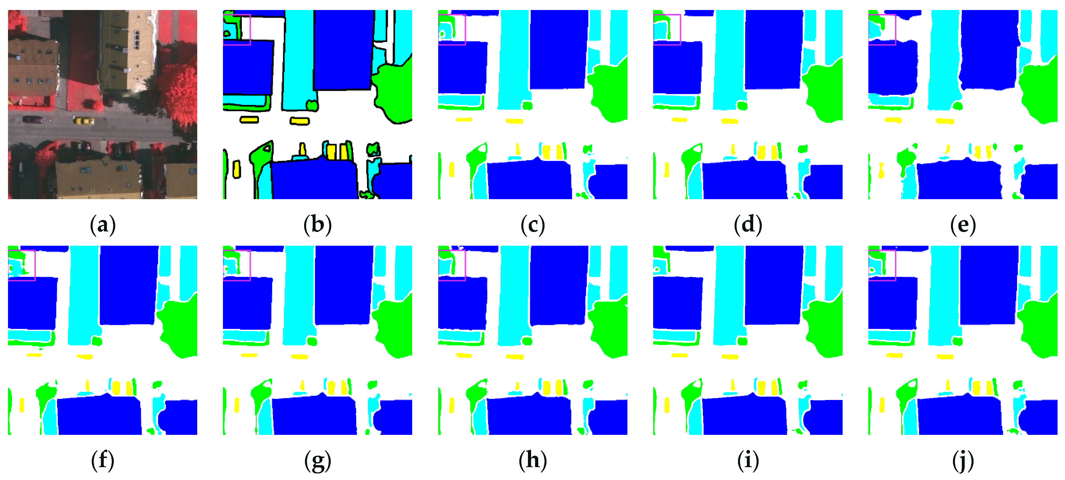
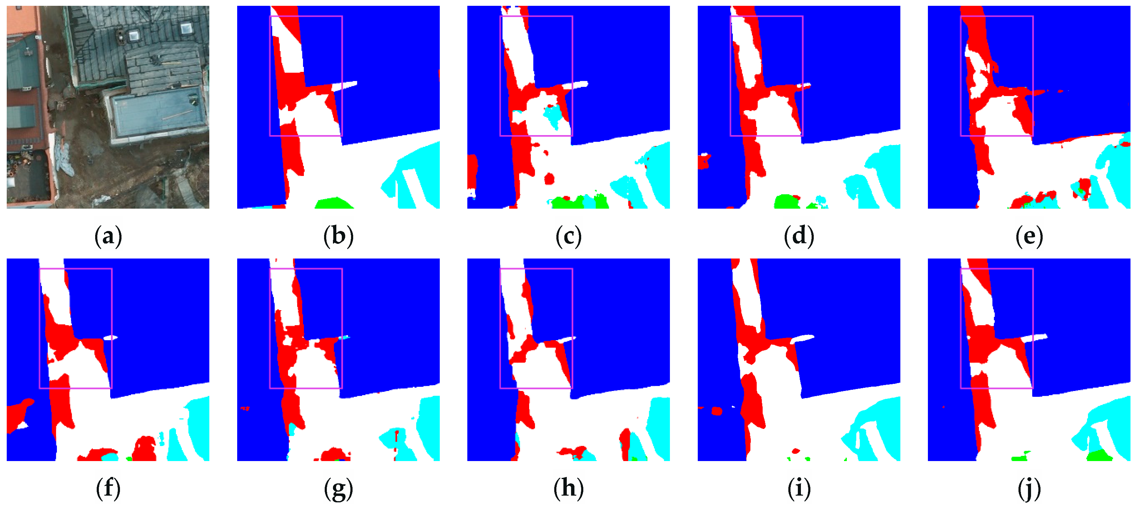
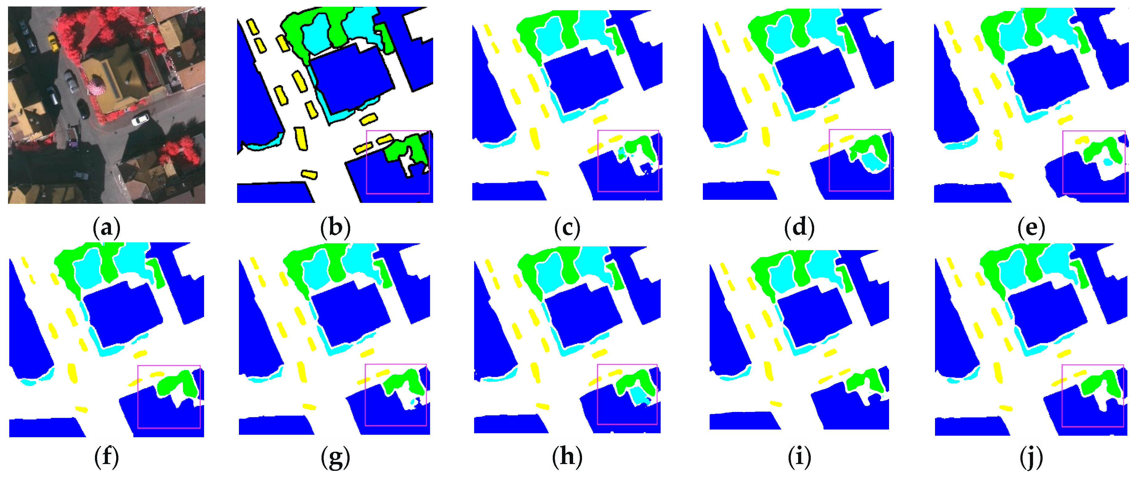
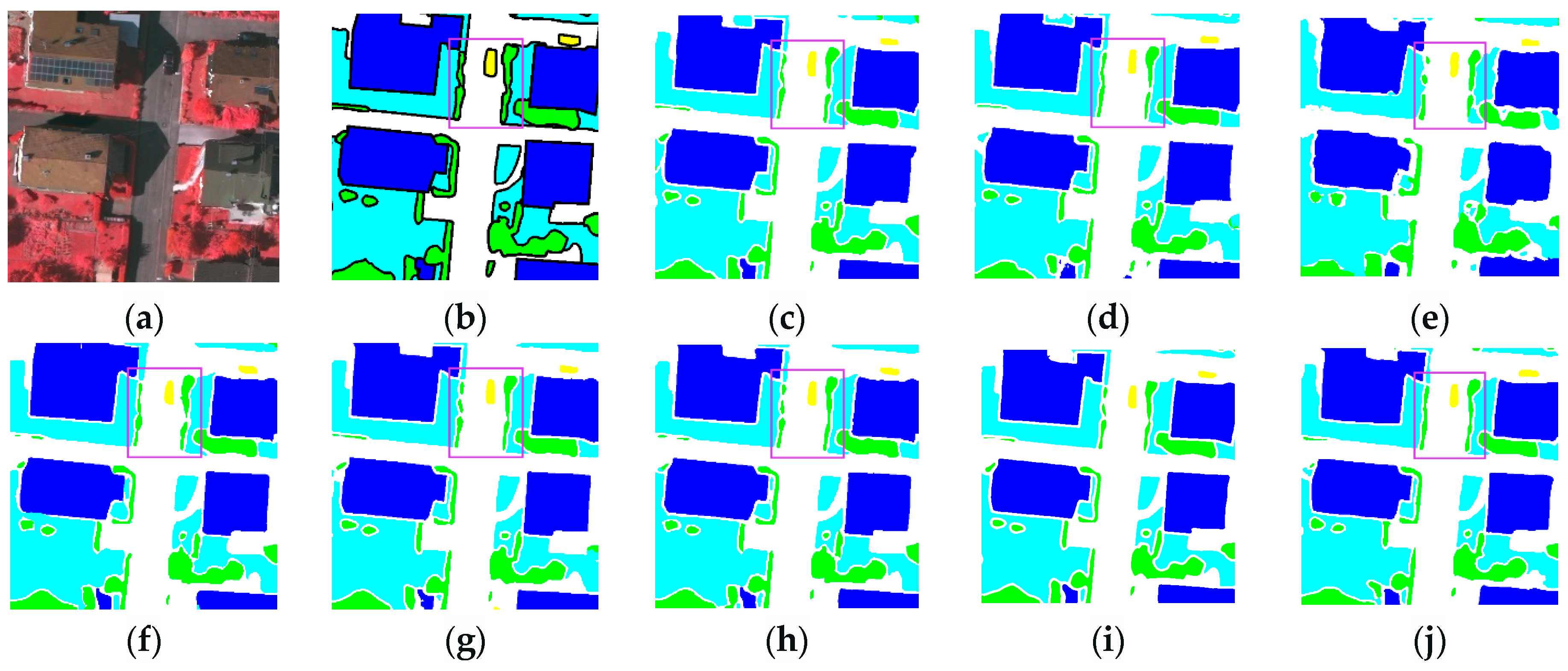
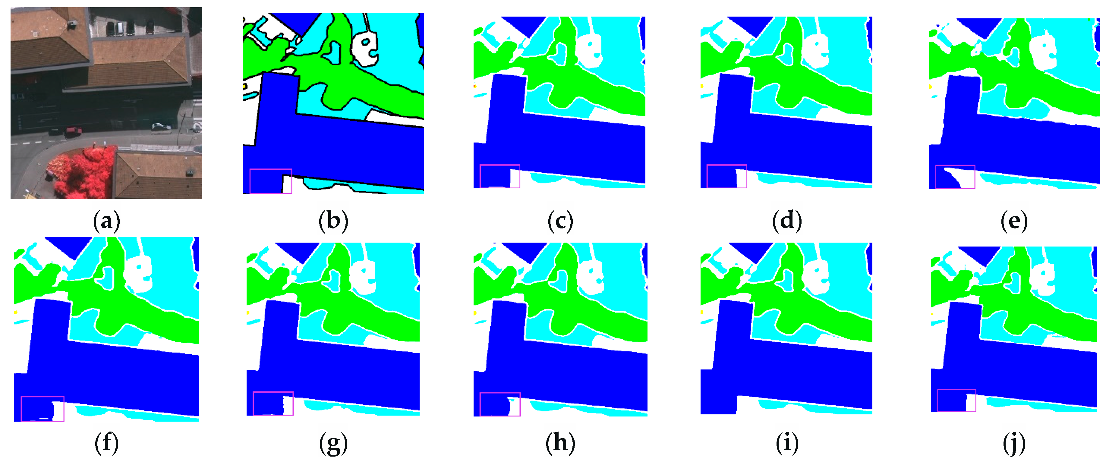
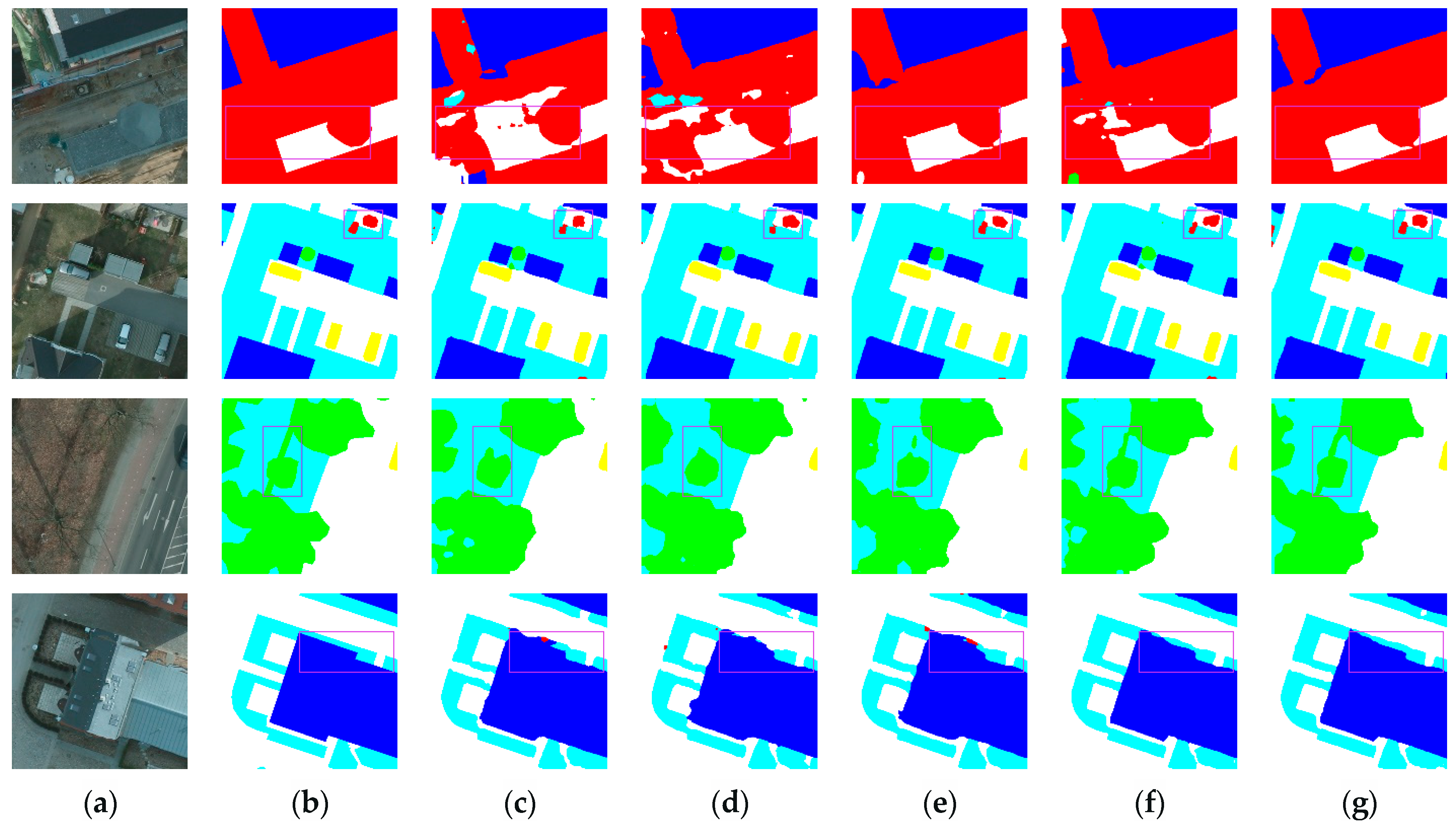
3.3.2. Renderings Analysis
3.3.3. Ablation Experiments Analysis
3.3.4. Dilation Rates Analysis of ASPP+ Module
3.3.5. Comparative Analysis of Activation Functions
4. Discussion
5. Conclusions
Author Contributions
Funding
Data Availability Statement
Acknowledgments
Conflicts of Interest
References
- Xu, S.; Pan, X.; Li, E.; Wu, B.; Bu, S.; Dong, W.; Xiang, S.; Zhang, X. Automatic Building Rooftop Extraction from Aerial Images via Hierarchical RGB-D Priors. IEEE Trans. Geosci. Remote Sens. 2018, 56, 7369–7387. [Google Scholar] [CrossRef]
- Long, J.; Shelhamer, E.; Darrell, T. Fully Convolutional Networks for Semantic Segmentation. In Proceedings of the IEEE Conference on Computer Vision and Pattern Recognition, Boston, MA, USA, 7–12 June 2015; pp. 3431–3440. [Google Scholar]
- Ronneberger, O.; Fischer, P.; Brox, T. U-net: Convolutional Networks for Biomedical Image Segmentation. In Proceedings of the Medical Image Computing and Computer-Assisted Intervention–MICCAI 2015: 18th International Conference, Proceedings, Part III 18, Munich, Germany, 5–9 October 2015; Springer: Cham, Switzerland, 2015; pp. 234–241. [Google Scholar]
- Badrinarayanan, V.; Kendall, A.; Cipolla, R. Segnet: A Deep Convolutional Encoder-Decoder Architecture for Image Segmentation. IEEE Trans. Pattern Anal. Mach. Intell. 2017, 39, 2481–2495. [Google Scholar] [CrossRef] [PubMed]
- Zhao, H.; Shi, J.; Qi, X.; Wang, X.; Jia, J. Pyramid Scene Parsing Network. In Proceedings of the IEEE Conference on Computer Vision and Pattern Recognition, Honolulu, HI, USA, 21–26 July 2017; pp. 2881–2890. [Google Scholar]
- Chen, L.C.; Papandreou, G.; Kokkinos, I.; Murphy, K.; Yuille, A.L. Semantic image segmentation with deep convolutional nets and fully connected crfs. arXiv 2014, arXiv:1412.7062. [Google Scholar]
- Chen, L.C.; Papandreou, G.; Kokkinos, I.; Murphy, K.; Yuille, A.L. DeepLab: Semantic Image Segmentation with Deep Convolutional Nets, Atrous Convolution, and Fully Connected CRFs. IEEE Trans. Pattern Anal. Mach. Intell. 2017, 40, 834–848. [Google Scholar] [CrossRef] [PubMed]
- Chen, L.C.; Papandreou, G.; Schroff, F.; Adam, H. Rethinking Atrous Convolution for Semantic Image Segmentation. arXiv 2017, arXiv:1706.05587. [Google Scholar]
- Chen, L.C.; Zhu, Y.; Papandreou, G.; Schroff, F.; Adam, H. Encoder-Decoder with Atrous Separable Convolution for Semantic Image Segmentation. In Proceedings of the Computer Vision—ECCV 2018, Munich, Germany, 8–14 September 2018; Ferrari, V., Hebert, M., Sminchisescu, C., Weiss, Y., Eds.; Springer: Cham, Switzerland, 2018; pp. 833–851. [Google Scholar]
- Ding, L.; Tang, H.; Bruzzone, L. LANet: Local Attention Embedding to Improve the Semantic Segmentation of Remote Sensing Images. IEEE Trans. Geosci. Remote Sens. 2020, 59, 426–435. [Google Scholar] [CrossRef]
- Li, R.; Zheng, S.; Zhang, C.; Duan, C.; Su, J.; Wang, L.; Atkinson, P.M. Multiattention Network for Semantic Segmentation of Fine-Resolution Remote Sensing Images. IEEE Trans. Geosci. Remote Sens. 2021, 60, 5607713. [Google Scholar] [CrossRef]
- Xu, J.; Xiong, Z.; Bhattacharyya, S.P. PIDNet: A Real-Time Semantic Segmentation Network Inspired by PID Controllers. In Proceedings of the IEEE/CVF Conference on Computer Vision and Pattern Recognition, Vancouver, BC, Canada, 17–24 June 2023; pp. 19529–19539. [Google Scholar]
- Xu, M.; Wang, W.; Wang, K.; Dong, S.; Sun, P.; Sun, J.; Luo, G. Vision Transformers (ViT) Pretraining on 3D ABUS Image and Dual-CapsViT: Enhancing ViT Decoding via Dual-Channel Dynamic Routing. In Proceeding of the IEEE International Conference on Bioinformatics and Biomedicine (BIBM), Istanbul, Turkiye, 5–8 December 2023; pp. 1596–1603. [Google Scholar]
- Zheng, S.; Lu, J.; Zhao, H.; Zhu, X.; Luo, Z.; Wang, Y.; Fu, Y.; Feng, J.; Xiang, T.; Torr, P.H.; et al. Rethinking Semantic Segmentation from a Sequence-to-Sequence Perspective with Transformers. In Proceedings of the IEEE/CVF Conference on Computer Vision and Pattern Recognition, Nashville, TN, USA, 20–25 June 2021; pp. 6881–6890. [Google Scholar]
- Strudel, R.; Garcia, R.; Laptev, I.; Schmid, C. Segmenter: Transformer for Semantic Segmentation. In Proceedings of the IEEE/CVF International Conference on Computer Vision, Montreal, QC, Canada, 10–17 October 2021; pp. 7242–7252. [Google Scholar]
- Xie, E.; Wang, W.; Yu, Z.; Anandkumar, A.; Alvarez, J.M.; Luo, P. SegFormer: Simple and Efficient Design for Semantic Segmentation with Transformers. Adv. Neural Inf. Process. Syst. 2021, 34, 12077–12090. [Google Scholar]
- He, X.; Zhou, Y.; Zhao, J.; Zhang, D.; Yao, R.; Xue, Y. Swin Transformer Embedding UNet for Remote Sensing Image Semantic Segmentation. IEEE Trans. Geosci. Remote Sens. 2022, 60, 4408715. [Google Scholar] [CrossRef]
- Wang, L.; Li, R.; Zhang, C.; Fang, S.; Duan, C.; Meng, X.; Atkinson, P.M. UNetFormer: A UNet-Like Transformer for Efficient Semantic Segmentation of Remote Sensing Urban Scene Imagery. ISPRS J. Photogramm. Remote Sens. 2022, 190, 196–214. [Google Scholar] [CrossRef]
- Zhang, C.; Jiang, W.; Zhang, Y.; Wang, W.; Zhao, Q.; Wang, C. Transformer and CNN Hybrid Deep Neural Network for Semantic Segmentation of Very-High-Resolution Remote Sensing Imagery. IEEE Trans. Geosci. Remote Sens. 2022, 60, 4408820. [Google Scholar] [CrossRef]
- Hou, Q.; Zhou, D.; Feng, J. Coordinate Attention for Efficient Mobile Network Design. In Proceedings of the IEEE Conference on Computer Vision and Pattern Recognition (CVPR), Nashville, TN, USA, 20–25 June 2021; pp. 13708–13717. [Google Scholar]
- Ma, N.; Zhang, X.; Sun, J. Funnel Activation for Visual Recognition. In Proceedings of the European Conference on Computer Vision (ECCV), Glasgow, UK, 23–28 August 2020; pp. 351–368. [Google Scholar]
- Rottensteiner, F.; Sohn, G.; Gerke, M.; Wegner, J.D.; Breitkopf, U.; Jung, J. Results of the ISPRS Benchmark on Urban Object Detection and 3D Building Reconstruction. ISPRS J. Photogramm. Remote Sens. 2014, 93, 256–271. [Google Scholar] [CrossRef]
- Lyu, Y.; Vosselman, G.; Xia, G.S.; Yilmaz, A.; Yang, M.Y. UAVid: A Semantic Segmentation Dataset for UAV Imagery. ISPRS J. Photogramm. Remote Sens. 2020, 165, 108–119. [Google Scholar] [CrossRef]
- He, K.; Zhang, X.; Ren, S.; Sun, J. Deep Residual Learning for Image Recognition. In Proceedings of the IEEE Conference on Computer Vision and Pattern Recognition, Las Vegas, NV, USA, 27–30 June 2016; pp. 770–778. [Google Scholar]
- Wang, P.; Chen, P.; Yuan, Y.; Liu, D.; Huang, Z.; Hou, X.; Cottrell, G. Understanding Convolution for Semantic Segmentation. In Proceedings of the IEEE Winter Conference on Applications of Computer Vision (WACV), Lake Tahoe, NV, USA, 12–15 March 2018; pp. 1451–1460. [Google Scholar]
- Maas, A.L.; Hannun, A.Y.; Ng, A.Y. Rectifier Nonlinearities Improve Neural Network Acoustic Models. Proc. ICML 2013, 30, 3. [Google Scholar]
- Glorot, X.; Bordes, A.; Bengio, Y. Deep Sparse Rectifier Neural Networks. J. Mach. Learn Res. 2011, 15, 315–323. [Google Scholar]
- He, K.; Zhang, X.; Ren, S.; Sun, J. Delving Deep into Rectifiers: Surpassing Human-Level Performance on Imagenet Classification. In Proceedings of the IEEE International Conference on Computer Vision, Santiago, Chile, 7–13 December 2015; pp. 1026–1034. [Google Scholar]
- Kingma, D.P.; Ba, J. Adam: A Method for Stochastic Optimization. arXiv 2014, arXiv:1412.6980. [Google Scholar]
- Clevert, D.; Unterthiner, T.; Hochreiter, S. Fast and Accurate Deep Network Learning by Exponential Linear Units (elus). arXiv 2015, arXiv:1511.07289. [Google Scholar]
- Misra, D. Mish: A Self Regularized Non-monotonic Activation Function. arXiv 2019, arXiv:1908.08681. [Google Scholar]
- Chen, Y.; Dai, X.; Liu, M.; Chen, D.; Yuan, L.; Liu, Z. Dynamic Relu. In Proceedings of the European Conference on Computer Vision, Online, 23–28 August 2020; pp. 351–367. [Google Scholar]


| Method | Parameters(M) | PA/% | F1/% | MIoU/% | Kappa |
|---|---|---|---|---|---|
| UNet | 17.27 | 92.66 | 78.08 | 71.35 | 0.9492 |
| SegNet | 29.45 | 92.61 | 77.61 | 70.84 | 0.9491 |
| DeepLab V3+ | 21.94 | 90.00 | 72.24 | 64.17 | 0.8913 |
| LANet | 23.81 | 93.29 | 78.77 | 72.29 | 0.9496 |
| MANet | 35.86 | 92.06 | 76.89 | 69.86 | 0.9256 |
| UNetFormer | 11.28 | 91.23 | 75.01 | 67.51 | 0.9138 |
| Swin-CNN | 66 | 94.56 | 81.68 | 76.62 | 0.9521 |
| ASPP+-LANet | 27.46 | 95.53 | 82.57 | 77.81 | 0.9552 |
| Method | Parameters(M) | PA/% | F1/% | MIoU/% | Kappa |
|---|---|---|---|---|---|
| UNet | 17.27 | 98.03 | 81.83 | 79.53 | 0.9637 |
| SegNet | 29.45 | 96.82 | 80.21 | 76.77 | 0.9433 |
| DeepLab V3+ | 21.94 | 92.77 | 73.31 | 67.33 | 0.8721 |
| LANet | 23.81 | 97.55 | 80.82 | 77.77 | 0.9465 |
| MANet | 35.86 | 98.08 | 81.81 | 79.55 | 0.9677 |
| UNetFormer | 11.28 | 96.73 | 80.08 | 76.52 | 0.9429 |
| Swin-CNN | 66 | 97.98 | 81.66 | 78.86 | 0.9625 |
| ASPP+-LANet | 27.46 | 98.24 | 81.99 | 79.83 | 0.9689 |
| Method | PA/% | F1/% | MIoU/% |
|---|---|---|---|
| LANet | 93.29 | 78.77 | 72.29 |
| LANet + ASPP | 93.71 | 79.46 | 73.29 |
| LANet + ASPP+ | 93.86 | 79.80 | 73.75 |
| LANet + FReLU | 95.22 | 82.05 | 77.06 |
| ASPP+-LANet | 95.53 | 82.57 | 77.81 |
| Method | PA/% | F1/% | MIoU/% |
|---|---|---|---|
| LANet | 97.55 | 80.82 | 77.77 |
| LANet + ASPP | 97.77 | 81.31 | 78.65 |
| LANet + ASPP+ | 97.80 | 81.42 | 78.79 |
| LANet + FReLU | 97.76 | 81.30 | 78.59 |
| ASPP+-LANet | 98.24 | 81.99 | 79.83 |
| Dilation Rate | PA/% | F1/% | MIoU/% |
|---|---|---|---|
| (1, 2, 4, 6, 8) | 95.50 | 82.51 | 77.74 |
| (1, 2, 4, 8, 12) | 95.53 | 82.57 | 77.81 |
| (1, 3, 6, 12, 18) | 95.47 | 82.39 | 77.60 |
| (1, 3, 8, 16, 18) | 95.46 | 82.51 | 77.74 |
| (1, 3, 8, 18, 24) | 95.51 | 82.52 | 77.73 |
| Activation Function | PA/% | F1/% | MIoU/% |
|---|---|---|---|
| LANet + LeakyReLU [26] | 93.34 | 78.73 | 72.31 |
| LANet + PReLU [28] | 94.37 | 80.65 | 74.94 |
| LANet + ELU [30] | 90.23 | 72.58 | 64.83 |
| LANet + Mish [31] | 89.99 | 73.50 | 65.74 |
| LANet + DY-ReLU [32] | 94.10 | 80.26 | 74.40 |
| LANet + FReLU | 95.22 | 82.05 | 77.06 |
Disclaimer/Publisher’s Note: The statements, opinions and data contained in all publications are solely those of the individual author(s) and contributor(s) and not of MDPI and/or the editor(s). MDPI and/or the editor(s) disclaim responsibility for any injury to people or property resulting from any ideas, methods, instructions or products referred to in the content. |
© 2024 by the authors. Licensee MDPI, Basel, Switzerland. This article is an open access article distributed under the terms and conditions of the Creative Commons Attribution (CC BY) license (https://creativecommons.org/licenses/by/4.0/).
Share and Cite
Hu, L.; Zhou, X.; Ruan, J.; Li, S. ASPP+-LANet: A Multi-Scale Context Extraction Network for Semantic Segmentation of High-Resolution Remote Sensing Images. Remote Sens. 2024, 16, 1036. https://doi.org/10.3390/rs16061036
Hu L, Zhou X, Ruan J, Li S. ASPP+-LANet: A Multi-Scale Context Extraction Network for Semantic Segmentation of High-Resolution Remote Sensing Images. Remote Sensing. 2024; 16(6):1036. https://doi.org/10.3390/rs16061036
Chicago/Turabian StyleHu, Lei, Xun Zhou, Jiachen Ruan, and Supeng Li. 2024. "ASPP+-LANet: A Multi-Scale Context Extraction Network for Semantic Segmentation of High-Resolution Remote Sensing Images" Remote Sensing 16, no. 6: 1036. https://doi.org/10.3390/rs16061036
APA StyleHu, L., Zhou, X., Ruan, J., & Li, S. (2024). ASPP+-LANet: A Multi-Scale Context Extraction Network for Semantic Segmentation of High-Resolution Remote Sensing Images. Remote Sensing, 16(6), 1036. https://doi.org/10.3390/rs16061036