Suitability Index for the Placement of Solar Plants Based on Inequality Measurements and on Satellite Images

Abstract

The selection of a certain location for the placement of a solar facility depends on the solar resource availability, which is generally assessed though exceedance probabilities. However, the choice of the specific exceedance probability is arbitrary and the assessment will be different depending on the choice taken. Furthermore, exceedance probabilities do not reflect seasonal variability, which affects radiation availability. Therefore, in this work we present a new index, the suitability index based on Theil (SIT), which allows us to assess with a single value the degree of suitability of a site for installing a solar plant. Obtained from the Theil index, it considers the availability of the resource and its seasonal variability, based as it is on the proportion of the given radiation in each month. As we will see, the new index is clearly more sensitive to the amount of radiation expressed in terms of the 50th percentile than to the variability, as given by the interquartile range. This is a quality to be pondered since scarcity of radiation will always be a greater disadvantage for a solar installation than high variability. The results obtained in the study, grounded in the application of satellite images, show that the index adequately reflects the radiation characteristics in the study area. The territory is broken into areas associated with such characteristics through a cluster analysis, so that geographical and economic elements can be considered when choosing the final location for a solar installation. Furthermore, the new index may include the effects of energy storage during the months in which a certain demand is exceeded.

1. Introduction

In order to assess the availability of the resource in a solar installation, two elements need to be considered: the amount of radiation and its variability. Indeed, both aspects are of great consequence, as some locations have large amounts of the resource, but are affected by high variability, and others have a scarce, but yearly stable, resource.

Although there are different variability indices available in the literature, such as the interquartile range, the variation coefficient, or the seasonality index, variability tends to be expressed by time series evolution (for example, time series of the photovoltaic potential or of the solar availability [1,2]). Variability is also represented by non-time-dependent methods, such as the cumulative distribution [3], the PDF or probability density function [4], and other formulations taken from the standard deviation [5]. Time series may also be distributed into classes of a scheme to assess temporal variability following some measure of irradiance variability [6] per cloud condition, which also affects variability. Temporal autocorrelation and class distribution are combined in [7], which includes a study of the autocorrelation of temporal series of the per class clear-sky index. This implies the formation of a categorization, which imposes restrictions on the study. Besides, autocorrelation only measures the level of correlation between the values of the time series and the values of the series moved a certain period, but not the variations in irradiance at different times and, therefore, the need for storage.

Furthermore, if standard deviations are used for the assessment, the fluctuation of the worst variations are disregarded. Thus, exceedance probabilities of these variations may be a better method to assess the availability of the solar resource [8,9]. They express the probability of exceeding a certain energy value; then, an exceedance probability of 95% (value P95) implies that the solar plant annual production is exceeded 95% of the time. This P95 refers to the 5th percentile of the annual production dataset. Then, viability of a solar installation project depends on the worst irradiance conditions reaching the design site (the cases in which there is a smaller amount of the solar resource). Three scenarios are recommended in [10] for evaluating the viability of a project corresponding to different exceeding probabilities (P50, associated with percentile 50, P90, associated with percentile 10, and P99, associated with percentile 1).

On the other hand, long datasets are required to assess the exceedance probabilities of the solar resource. In [11] and in [12], at least 10-year datasets are recommended for the solar irradiation series, which may be based on ground measurements, on satellite data, or on a combination of both [13,14,15].

Spatial and historical time series of solar radiation have undoubtedly increased along the course of time. However, they are still limited, and users find it difficult to obtain long-term high-quality terrestrial databases. Nowadays, data taken from satellites are considered a reliable source of information of solar irradiance and resource availability [16,17,18]. The methodology to analyze the solar radiation components drawn from satellite images has evolved from the first scholarship [19,20,21] to present studies [22,23,24].

There is no question that variability in solar resource is an economic problem that reduces the planning horizon [25] and increases the storage needs [26,27,28,29]. In fact, there is a wide range of economic indices that assess the solar projects’ viability due to the production rate discontinuity. For instance, the ratio inventory–sales estimates the cost of uncertainty, that is, the final storage price of the solar resource [30]. Other indices are based on the standard of self-sufficiency, such as the self-consumption ratio (SCR) or the self-sufficiency rate (SSR). Further indices consider a proportion of the energy-consumer demand that is met locally, or the time needed to recover the initial investment of the project, as the simple payback time (SPBT) [31]. Also, we have the levelized storage cost (LCOS), which includes the total energy drawn from storage considering the cost of charging cost [32], or the levelized cost of energy (LCOE), which comprises costs that occur during the useful life of the project. In this sense, both the life-cycle assessment and the cash-flow analysis can be used [33]

However, in the studies which assess the convenience of settling solar installations, there is no synthetic index that combines the two basic elements needed for assessing the availability of the resource (the amount of radiation and its variability). Financial analysis can furnish us with this index. First, none of the existing indices include the danger of not storing energy, the real opportunity cost and, therefore, the genuine value of energy. Besides, in finances, the return–risk binomial is assessed. In the financial field, the availability is the return expectation, and the variability is the risk (or variation) of that return. Investors could accept some level of risk, expecting to obtain higher returns. The choice of the investor will depend on their attitude towards risk. More risk should be counterbalanced with more than proportional returns just to keep a risk-averse investor indifferent [34]. This return–risk binomial then introduces new possible choices, given that some locations have a large amount of the resource, but with high variability and, on the other hand, there are locations where there is scarce resource despite being rather stable throughout the year.

This work aims at proposing this new index, which evaluates the degree of goodness of a location to place a solar plant based on the quantity and the solar resource variability. To achieve this, a well-known index, widely used to estimate inequality of income, the Theil index, will be adapted to solar resource inequality. This index is based on the entropy coefficient of the income distribution of a given population, subtracting from the maximum entropy the entropy corresponding to the income distribution of the given population. Furthermore, a cluster analysis based on the proposed index is carried out, so that regions in which the behavior of the index is similar are described. The new index will facilitate the possible choice of locations of solar plants. Finally, the values of the new suitability index, considering the possibility of storing energy in months in which there is surplus radiation for a given demand, are determined. The work uses the direct normal irradiance (DNI). It stands for a concentrated solar power (CSP) technology, although the methodology could also be applied for a photovoltaic (PV) technology to the global horizontal irradiance (GHI).

The structure of the article is as follows: firstly, in the material and methods section, the datasets used to carry out the study are described, and a brief physical description of the Iberian Peninsula is given. The methods normally used to assess the investment risk associated with the resource availability are also indicated (exceedance probabilities, interquartile range, or the average–variance binomial). Subsequently, the adaptations made to the Theil index to implement the new index proposed are pointed out, providing an instrument which estimates the availability of the solar resource at each point in the study area. Likewise, the methodologies used in the cluster analysis, which is carried out based on the previously implemented index, are drawn. Finally, an explanation of how the radiation curve has been modified throughout the year at each point in the area, considering the possibility of storing radiation in months with a surplus of the resource, is offered. Then, the results drawn by applying the proposed methodologies in the study area are discussed. In the last section, some conclusions of the work are drawn.

2. Material and Methods

2.1. Data

The monthly average values of DNI from 1 January 1983 to 31 December 2015, taken from EUMETSAT’s Satellite Application Facility on Climate Monitoring (CM-SAF) [35] have been applied to an area between −9.9°E and 3.9°E in longitude and 45.45°N and 34°N in latitude (the study region corresponds, therefore, to the Iberian Peninsula), with a resolution of 0.05° × 0.05°. According to the information provided by CM-SAF [36], the validation results of this product, as compared to the data from the measurements of baseline surface radiation network (BSRN) (1794 analyzed months), cast a slight bias of −0.9 W/m², the standard deviation is 21.9 W/m², and the mean absolute difference is 16.4 W/m². Details regarding the algorithm used for the generation of this product can be accessed in [37]. It is to be noted that, in May 2023, the latest edition of this data record (SARAH-3) was published, with slightly better validation results and a temporal coverage from 1983 to now.

In Figure 1, the physical map of the Iberian Peninsula is displayed. As for the orography, the Iberian Peninsula has some major mountain ranges. The Pyrenees is the neck of land between Spain and France. The Pyrenees continue west to the Cantabrian Mountains, running for 480 km. The Iberian System or Sistema Ibérico is a massif of rugged and high mountains in the east of the centrally placed tableland; it consists of the main basin of the Iberian Peninsula between the Mediterranean Sea and the Atlantic Ocean. The Central System mountains or Sistema Central is in the middle of the Iberian Peninsula. The mountain range of Sierra Morena has a low average height between 800 and 1000 m. The mountain range of the Baetic System spans 600 km in the south of the Iberian Peninsula from the Bay of Cadiz to the Valencia region. In the Iberian Peninsula, there are also plateaus such as the Meseta Central or Central Plateau, which is a vast elevated region in the interior surrounded by mountainous massifs, which divides the Meseta from the rest of the Peninsula. Two important valleys must be highlighted: (a) the Guadalquivir River basin, which flows from east to west and drains into the Gulf of Cadiz, in the south of the peninsula; and (b) the Ebro River basin, which spans 930 km from Cantabria in northern Spain to the east-southeast. At its mouth, it forms a delta and flows into the Mediterranean Sea.

2.2. Methods Applied

2.2.1. Exceedance Probabilities and Interquartile Range

Firstly, the 90% exceedance probabilities of solar radiation associated with the 10th and 50th percentiles are, respectively, estimated. In this sense, in the study area, the average radiation for each point and each month (monthly values corresponding to 33 years of the data of DNI gathered) is calculated, and with these values, the corresponding percentiles in each point of the study area are determined.

Next, in order to estimate the seasonal variability within the study area, the interquartile range is estimated in each of these points. This range is defined as the difference between the 75th and 25th percentiles, so it gives an idea of the variation presented by the central values of the variable.

2.2.2. The Average and the Variance

In financial analysis, assets have a theoretical return free of risk (including the risk of inflation). This is a minimum return that investors will demand for accepting the delay of consumption while they are tied up by the investment. Usually, individuals will welcome some level of risk with the compensation of an expectation of drawing higher returns in the future. However, the investor attitude towards risk will affect their choice, and in economic theory this attitude is usually formalized by the utility function, a graph that relates the satisfaction degree that the individual associates with the possession of a commodity or a return with the quantity of that commodity or return. Each individual has a different risk aversion in each moment and place; it is a subjective feeling that may even be unconscious to him. This psychological principle may be reduced to the law of large numbers, but it introduces a broad element of arbitrariness; some will even say a “radical uncertainty” [38]. Theoretically, the expected utility of some project is a function of the return and the variance [39,40]. However, the final choice of best location to install a solar project depends on utility functions.

In the radiation resource, the expectation of return of an investment and the risk of radiation unavailability must be ascertained. The calculation of this mean–variance binomial has the advantage of not requiring an entire probability distribution, only the two moments mean–variance. Besides, radiation is a physical phenomenon, although, as previously explained, the decision maker can also take into account in this case their attitude towards risk.

2.2.3. Suitability Index Based on Theil

The objective of this work is twofold. On the one hand, a single index, based on satellite images, which serves us to assess the solar radiation availability both in terms of quantity and variability in the study area, is proposed. This index will serve as an estimator of the degree of suitability for installing a solar installation of each point, as far as the availability of solar radiation is concerned. On the other hand, given that the selection of a certain point of the area may not be easy, conditioned as it is by geographical and/or economic reasons, a cluster analysis is carried out. This cluster analysis provides us with different regions in which the behavior of the index is similar. Thus, large areas suitable for the installation of solar plants are determined. In addition to establishing suitable regions based on solar resource availability, the cluster analysis will allow us to assess the goodness of the proposed index, comparing the regions drawn with the climatic regions in the study area.

Regarding the first objective, the proposed index will be built from the Theil index, which is normally used to measure the inequality of the income earned by a population. This index is calculated by subtracting the entropy corresponding to the income distribution of the given population from the maximum entropy of the population.

The entropy coefficient of the income distribution of a given population is defined by [41] as:

$$H\left(y\right)=-{\sum }_{u=1}^N{y}_u\log y_u$$

(1)

where the number of individuals is $N$ and $y_u$ is the participation of individual $u$ in the total income of the population.

This coefficient is a measure of inequality that varies between 0 and $\log N$, two extreme cases that correspond to perfect inequality and perfect equality, respectively. There are other inequality indices, such as the Gini index, which assesses the statistical dispersion and the inequality among the different values of a distribution of frequencies [42]. But the generalized entropy class of coefficients, such as the Theil index, may be additively decomposed between and within any arbitrarily categorized subgroups of the population [43,44,45]. In [46], inequality is decomposed by subgroups that share certain characteristics such as date of birth, household dimensions, locality, occupation of the family members, or level of education. This decomposition capacity is very useful for our needs, as we will divide the territory into areas where the value of the index is similar.

The entropy coefficient is transformed, according to [47], into a measure of inequality by subtracting its value from its own maximum value.

$$T=\log N-H\left(y\right)$$

(2)

The Theil index shown in Equation (2), with convenient adaptations, can be used to define an index which allows us to assess with a single value the degree of suitability of the points of a certain area for the election of the placement of a solar plant. Indeed, to estimate the Theil coefficient at each point of the study area, we proceed as follows. (a) From the average monthly data taken for different years from CM SAF, monthly averages for all those years are obtained in each of the points of the study area. (b) At each point in the area, the entropy of the radiation distribution provided by the twelve values previously obtained is calculated using Equation (1). However, in order to achieve the abovementioned goal, this formulation is adapted to be able to assess the entropy at each point of the area. Thus, the inequality at the given point is no longer estimated by considering the participation of each individual (in this case, each month) in the total radiation collected over that point but by considering the participation of each month in the maximum total radiation collected in the entire study area. (c) The Theil coefficient, which measures inequality, and therefore variability, is estimated from Equation (2), where specific entropy is subtracted from the maximum entropy of the population. This maximum entropy corresponds to the logarithm of the size of the population given (the entropy of the distribution, previously calculated). In this case, the maximum DNI collected in the entire study area is also taken as the maximum entropy. With these adaptations, the Theil index will consider all the monthly radiation values existing in the study area, which will allow the values obtained for the different points to be comparable. On the other hand, the maximum value of the entire area taken as a reference allows us to assess the amount of radiation received. This turns the index not only into a measure of variability, but also of the degree of radiation received.

Therefore, in Equation (2), $\mathrm{l}\mathrm{o}\mathrm{g}N$ must be replaced with the maximum total radiation received in the entire study area, $N$ being the 12 months of the year, which are the individuals considered at each point. The $y_u$ of $H \left(y\right)$ is the participation of the $u$-th month in the maximum total radiation received throughout the study area. With these adaptations, the suitability index based on Theil (SIT) may be defined as:

$$SIT=\max DNI-{\sum }_{u=1}^N{y}_u\log y_u$$

(3)

2.2.4. Clustering Analysis

Once the index that allows us to estimate the degree of suitability of a location to install a solar plant is defined, a cluster analysis from the previously obtained index is carried out. For this analysis, the k-means procedure will be used, and to determine the best clusters number to be included, two methods will be applied: the Davies method and the silhouette method.

The k-means technique [48] consists of an algorithm for organizing data into clusters that minimizes the addition of the squared distances between each element in the cluster and its centroid. This k-means algorithm is applied in the following way: (a) some starting clusters are created randomly and their centroids determined; (b) the distance between these centroids and the data is calculated; (c) each value is allocated to the cluster that has the closest centroid; (d) these new data are used to obtain new centroids; and (e) finally, the method will be iterated until there is a convergence of the sum of the distances between the centroids of the cluster and the data.

Different methods to obtain the optimal clusters number could be applied. In this work, the Davies and silhouette methods are applied.

• The Davies method

The Davis–Bouldin index, defined in [49], determines the optimal clusters number by calculating the distances inside the clusters and between clusters. It is defined as:

$$DB=\frac{1}{N}{\sum }_{i=1}^N\underset{j\ne i}{\max }\left[\frac{{\sigma }_i+{\sigma }_j}{d\left(c_i,c_j\right)}\right]$$

(4)

where the clusters number is $N$, $c_x$ is the centroid of the cluster, ${\sigma }_x$ is the mean distance of all elements $x$ in the distance of the cluster to the centroid $c_x$, and $d\left(c_i,c_j\right)$ is the separation between the centroids.

Clustering algorithms aim to create groups with short distances within the cluster itself and large distances between different clusters. Thus, these algorithms will imply a small value of the Davies–Bouldin index.

The term $\underset{j\ne i}{\max }\left[\frac{{\sigma }_i+{\sigma }_j}{d\left(c_i,c_j\right)}\right]$ is the representation of the worst value for cluster $i$. Then, the optimum case is the one which yields the smallest value for the Davies–Bouldin index.

• The Silhouette method

Suggested by [50], it measures the consistency within clusters. A cluster plot is drawn with a silhouette that has a width value of $s\left(i\right), i=\mathrm{1,2},\dots , n$, which evidences the quality of the display of objects into clusters. Each individual object within the cluster is symbolized by $i$. For each individual, $i$, the value $s\left(i\right)$ is estimated from:

$$s\left(i\right)=\frac{b\left(i\right)-a\left(i\right)}{\max (a\left(i\right),b\left(i\right))}$$

(5)

where $a\left(i\right)$ represents the mean dissimilarity of the individual $i$ as compared to all other data in the same cluster and $b\left(i\right)$ is the smallest mean dissimilarity of $i$ to any other neighboring cluster, of which $i$ is not a part.

The value of $s\left(i\right)$ ranges from $[-1, 1]$. If $s\left(i\right) \approx +1$, the object i is considered correctly labelled in the group, due to the inequality $a\left(i\right)<<b\left(i\right)$. Conversely, when $s\left(i\right) \approx -1$, the object is mismatched as $a\left(i\right)>>b\left(i\right)$. Lastly, when $s\left(i\right) \approx 0$, $i$ is an intermediate point of two groups between two different groups, as happens when $a \left(i\right)=b\left(i\right)$.

The definition of the mean silhouette width, $ASW$, is:

$$ASW=\frac{1}{N}{\sum }_{i=1}^{n}s\left(i\right)$$

(6)

This analysis appraises the cluster structure quality, so the natural clusters number in a dataset may be resolved through silhouette plots and averages.

2.2.5. Storage

Another aim of this study is to assess the suitability of a location to satisfy a certain constant monthly energy demand expressed in terms of solar radiation. This is conducted by considering the odds of storing the excess energy during the months in which there is a radiation surplus. Then, the evolution of radiation at each point of the study territory is estimated, making use of the storage capacity, and considering these new values of the solar resource, the entropy, and the corresponding Theil index, with the already mentioned adaptations. In order to estimate this new evolution of the resource throughout the year at each point analyzed, the surpluses of radiation in each month are discarded. Then, radiation is made equal to the demand in the given months and, so, the total surplus is equally distributed between the months with radiation deficit.

3. Results

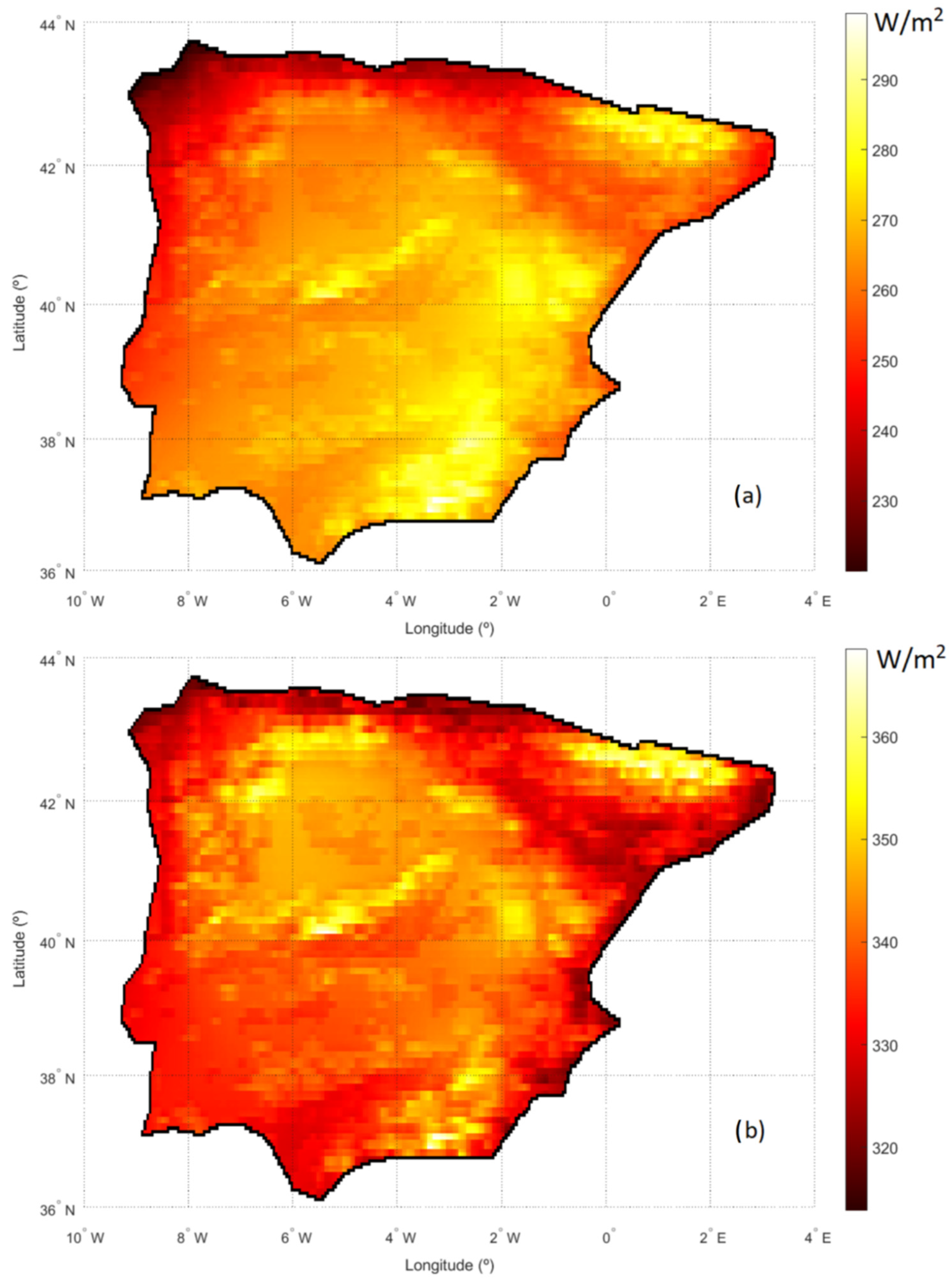
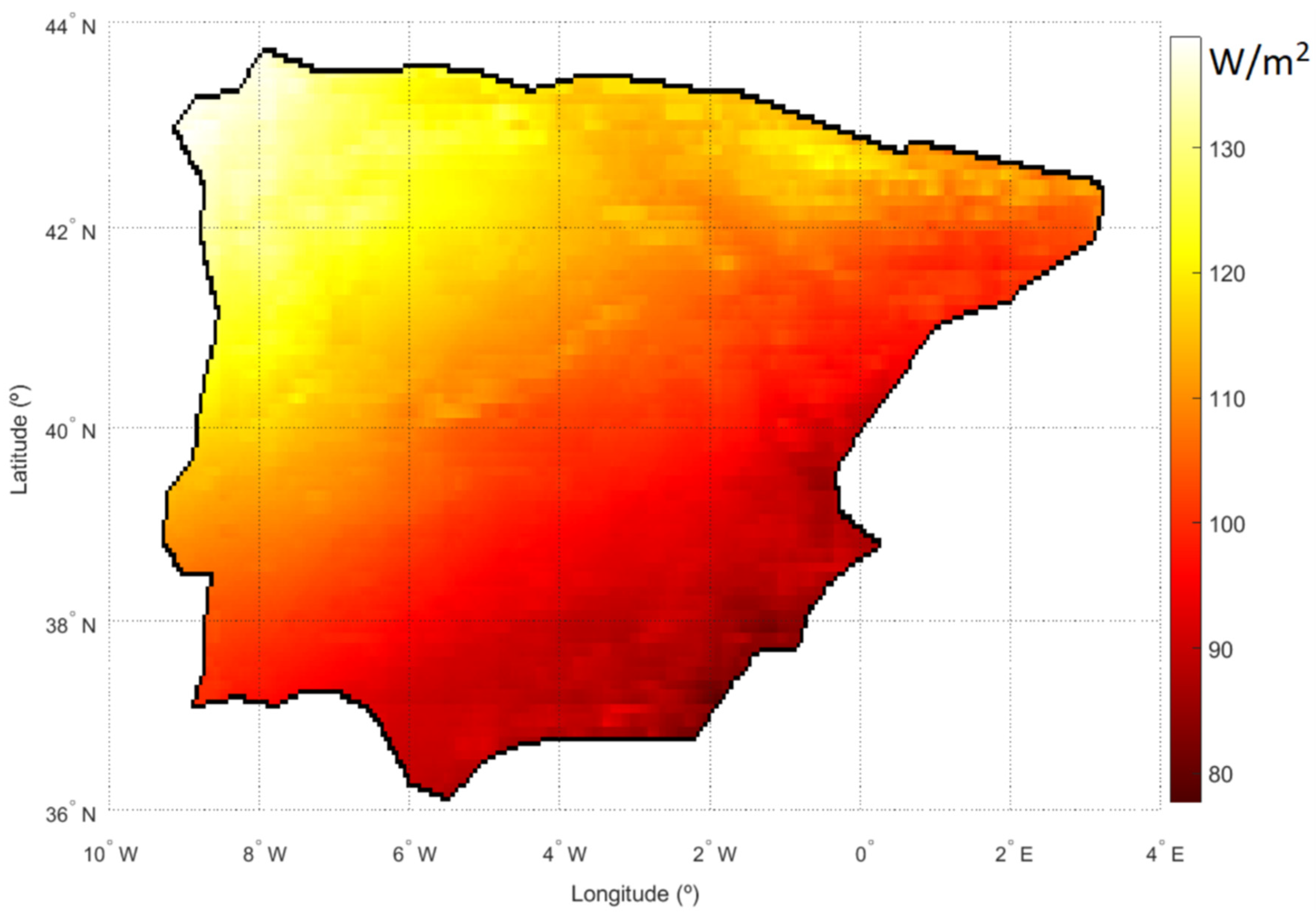
3.1. Exceedance Probabilities and Interquartile Range

As mentioned above, exceedance probabilities are widely used to estimate the suitability of a given place for the installation of a solar plant. Therefore, first, the 90% and 50% exceedance probabilities have been calculated for the data taken at each point in the study area (Figure 2). Given a direct relationship between solar radiation received and energy produced, radiation data are directly used. Let us remember that the 90% exceedance probability is linked to the value that is exceeded 90% of the time, that is, to the 10th percentile; similarly, the exceedance probability of 50% is associated with the 50th percentile. According to Figure 2a, the values associated with a probability of exceedance of 90% are higher in mountain areas (Pyrenees, Central System, Iberian Mountain Range, and Baetic System) and in the Iberian Peninsula southeast. Usually (90% of the time), high radiation values are exceeded in these areas. Therefore, considering only the availability of the solar resource, these would be the more favorable places for the installation of solar plants. On the contrary, in the north of the peninsula, if we frequently must exceed certain radiation values, these values must be much lower. Therefore, considering exclusively the availability of the resource, these would be the least suitable places for the location of a solar installation.

Figure 2b, which depicts the 50th percentile, associated with the exceedance probability of 50%, presents certain differences from Figure 2a. In fact, in the case of the 50th percentile, the southeast of the peninsula is no longer a particularly suitable area, and one of the least suitable areas appears to be, along with the north of the peninsula, the entire Mediterranean coast and the Ebro basin, which connects both areas of the northeast peninsula. The area of the eastern peninsula and the Guadalquivir valley (southwest of Spain) also appears unsuitable, although to a lesser extent than the previous regions. Consequently, taking one or the other exceedance probability leads to different results and, then, to great arbitrariness when selecting the best places for locating solar installations. This arbitrariness will be avoided using the suitability index proposed in this work. On the other hand, the use of exceedance probabilities does not explain the seasonal variability of radiation as only a value in the form of a percentile is provided, indicative of the available amount. However, the new proposed index takes this variability into account since it is prepared from the shares of each month in the total radiation.

The next step suggested in the material and methods section was the representation of the interquartile range corresponding to each point in the study area (Figure 3). The figure shows that the range presents a latitudinal behavior (the further we go to the north, the greater the variation) although with a very pronounced inclination due to the cascading entry of Atlantic fronts, especially in the northwest area of the peninsula.

3.2. Average and Variance

Figure 4 represents the average of the DNI (in W/m²) versus its variance throughout the study territory. Places that have high averages and low variances are the best places for the installation of solar plants; however, Figure 4 shows that, for a low variance, which is preferable for the risk-averse investor, all of the average spectrum is available. Then, the binominal average–variance is not a good method to ascertain the best points for the installation of solar plants as there are places with a high average and a low variance and with a low average and a high variance, not being comparable. Actually, there are several options equally preferable. These options may be depicted in indifference curves. Indifference curves for the user of PV solar plants—the points of the average–variance binomial that are indifferent for them—consist of positive slope curves where the return–risk binomials of solar radiation would be similarly preferable for a risk-averse investor. The arbitrage between consumers may decide between those different options. Furthermore, when different uses of energy are at different distances, and there are transport costs, the opportunity cost—the different possible usages of the installation regions—affects the final option [51,52] and a Von Thünen model [53] could be used.

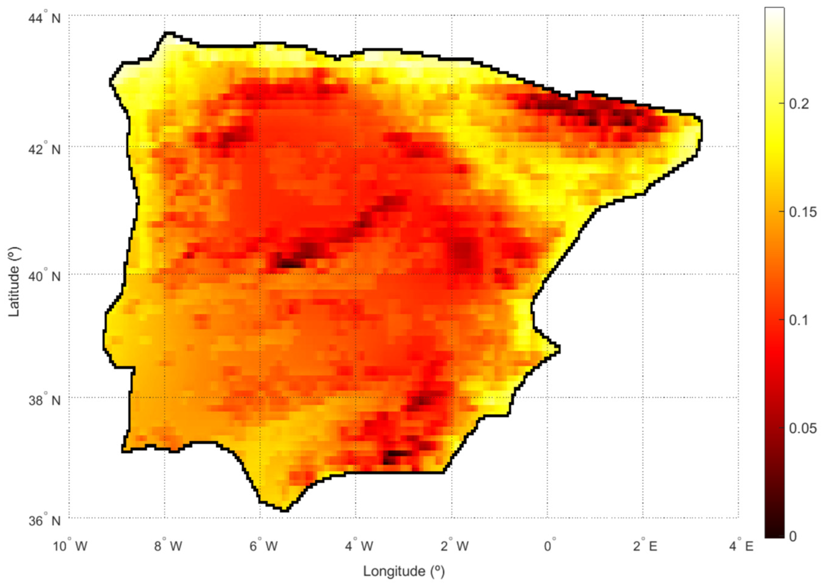
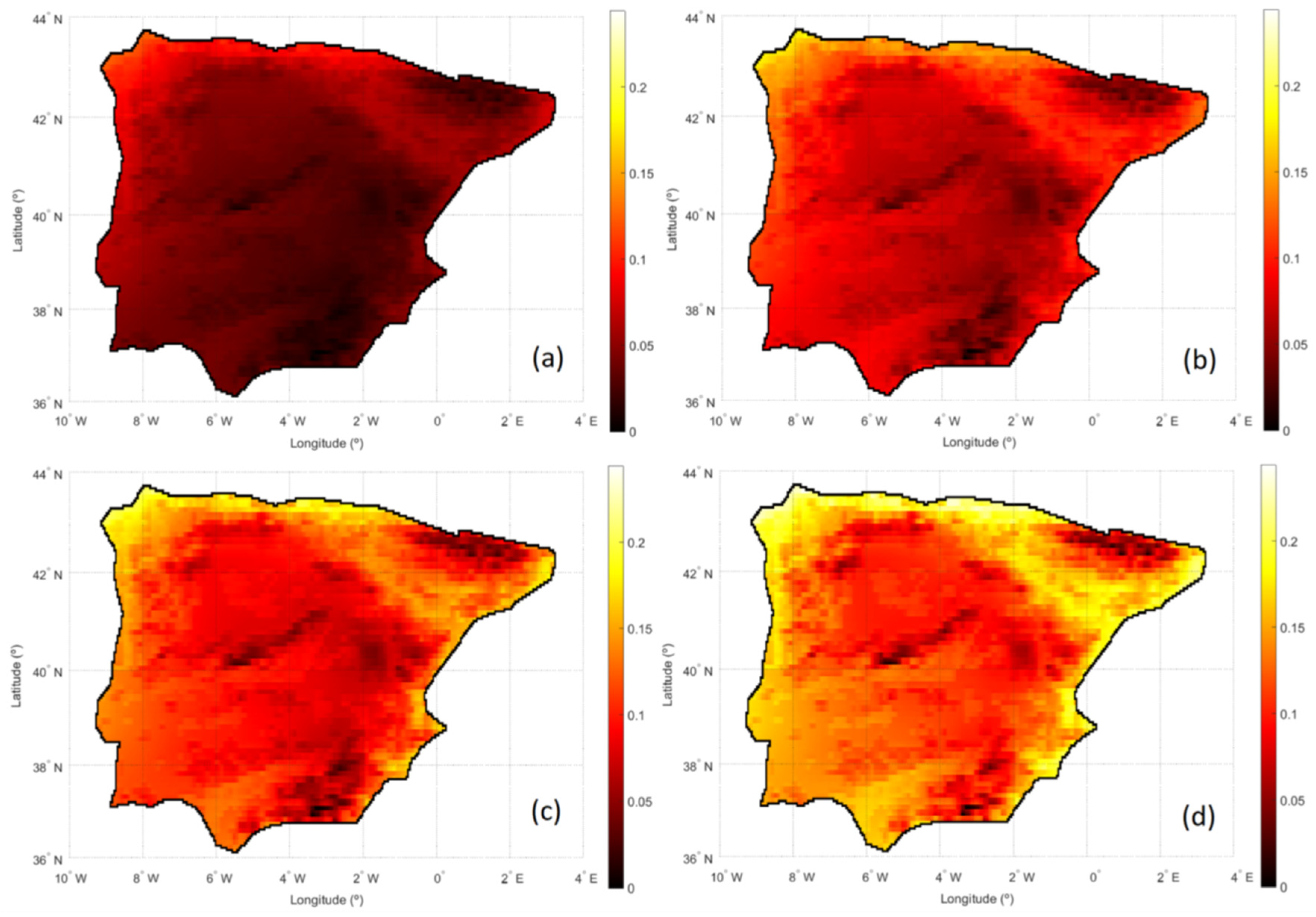
3.3. Suitability Index Based on Theil (SIT)

In accordance with expression (1) and the adaptations already discussed in the text, estimations of the new proposed suitability index (SIT) have been obtained for each point in the study area (Figure 5). As already indicated, values shown on the map are comparable, so that in the points where the index is lower, based solely on the criteria of availability of the solar resource (quantity and variability), the installation of a solar plant is more suitable.

According to Figure 5, the most suitable places coincide with the mountainous areas of the peninsula. In these areas, the radiation received is very high, as drawn from the average value shown in Figure 2b, though the variation throughout the year, reflected in terms of the interquartile range (Figure 3), depends on the area in which the mountainous area is located. However, these areas are not suitable for the installation of solar plants for geographical reasons. Next, the most suitable areas are those of the central fringe of the peninsula, dominated by a Mediterranean climate in its continental variant. In this climate, with hot summers and cold winters, radiation is high throughout the year, given that the mountain chains that isolate the central regions block the fronts arriving from the Atlantic. Therefore, this entire area may also be suitable for the installation of plants from a geographical point of view.

After the central peninsular area, the most suitable area for the installation of CPS plants is the Guadalquivir basin and the southern half of Portugal. There, the winds from the Atlantic bring cloud cover that limits the amount of radiation, as shown in Figure 2b, although variability throughout the year is not very pronounced (Figure 3). Finally, the least suitable area for the installation of solar plants is the entire northern part of the peninsula, as well as the Mediterranean coast and the Ebro basin. In the north of the peninsula, where, in contrast, variability is very high, the continuous entry of fronts throughout the year brings great cloudiness and, consequently, very low radiation values. The eastern coast of the peninsula, where variability is much lesser, has a Mediterranean climate, characterized in terms of precipitation by rainy winters and dry summers, along with variable precipitation in autumn and spring. This cloudiness explains the scarce suitability of the area, as seen in Figure 2b. Finally, the Ebro basin, where, according to Figure 3, variability changes along the basin, is located between two important mountain ranges (the Pyrenees to the northeast and the Iberian mountain range to the southwest). Then, it is also an unsuitable area for the installation of solar plants. Indeed, although it is an area with little rainfall, its location entails the presence of abundant fog that makes it unsuitable for the installation of solar plants. According to the above considerations, the SIT seems to be quite correlated with the mean value of radiation, represented in Figure 2b, whose similarity to Figure 5 is evident. This is to be expected, given that the suitability index based on Theil is calculated in an integrative manner, not giving greater weight to any radiation, so that the result should tend towards an average value. The fact that the correlation between the SIT and variability (Figure 3) is not so significant is a good quality of the index, since it seems more desirable that the average amount of radiation is high than that the variability is small. In any case, as against average radiation, the SIT is also affected by seasonality. In fact, in the extreme southwest of the peninsula, Figure 2b shows a similar behavior in much of the region (values close to 335 W/m²). However, according to Figure 3, this area exhibits different variabilities, expressed from the interquartile range. There, the variability increases from east to west, and this translates into an increasing suitability index (it is less suitable in that direction). The difference of sensitivity of the suitability index based on Theil with regard to the average radiation and variability will be discussed in more detail in Section 4.2, which provides a more detailed study of a group of selected sites.

4. Discussion

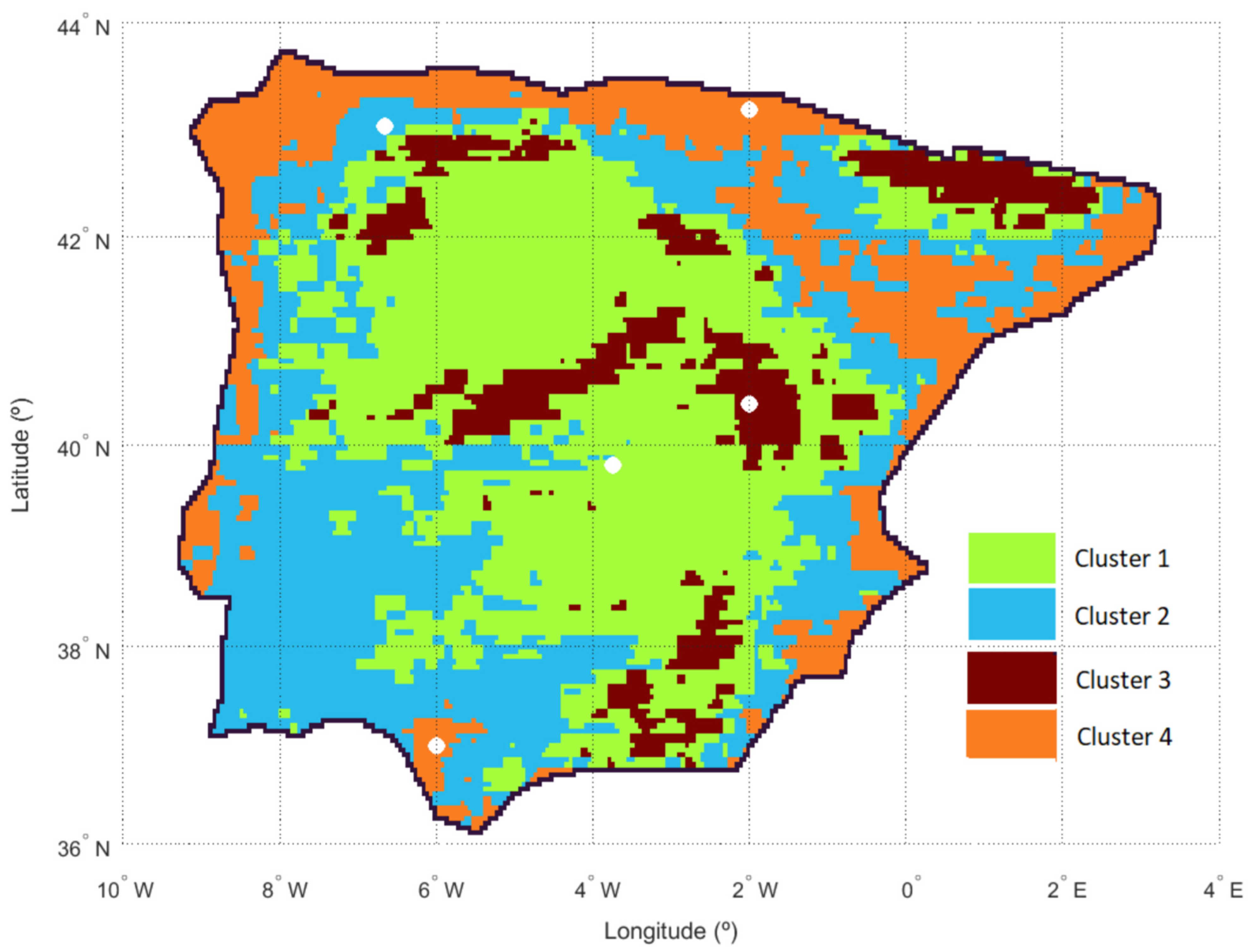
4.1. Clusters from the SIT

As previously indicated, two systems of determination of an optimal cluster number will be tested: the Davies method and the silhouette method. Applying Equation (2), the Davis–Bouldin index has been calculated for different numbers of clusters (n) (Figure 6a). Similarly, from Equation (3) the $ASW$ has been obtained for this number of clusters (Figure 6b). The variable used to carry out this study is the Theil index previously obtained.

According to Figure 6a, the best number of clusters is 9, which is the number of clusters for which a lower $DB$ is obtained. However, following the silhouette method, the optimal number is 2, the number of clusters for which the highest $ASW$ value is obtained. Given the disparity between both methods, an intermediate value (4 clusters) has been taken as optimal, which is also in accordance with the above explanation. Indeed, the four areas of suitability mentioned correspond to four areas where the behavior of the DNI is different, which allows the territory to be appropriately divided, as clearly observed in Figure 7, in which each cluster is determined by each different colour.

As indicated above, the variable used to divide the territory has been the SIT, so that within the various areas obtained, the behavior of this index is similar. This proves the adequacy of the index when it comes to characterizing the suitability of each of the points in the study area in terms of availability of the solar resource. Indeed, although the variant of the Theil index used in this article was calculated for each point in the space, the aforementioned capacity of the index to decompose into subgroups with common characteristics means that the inequality in the entire territory (different resource availability in the entire study area) can be decomposed into different regions with similar characteristics in terms of inequality (resource availability).

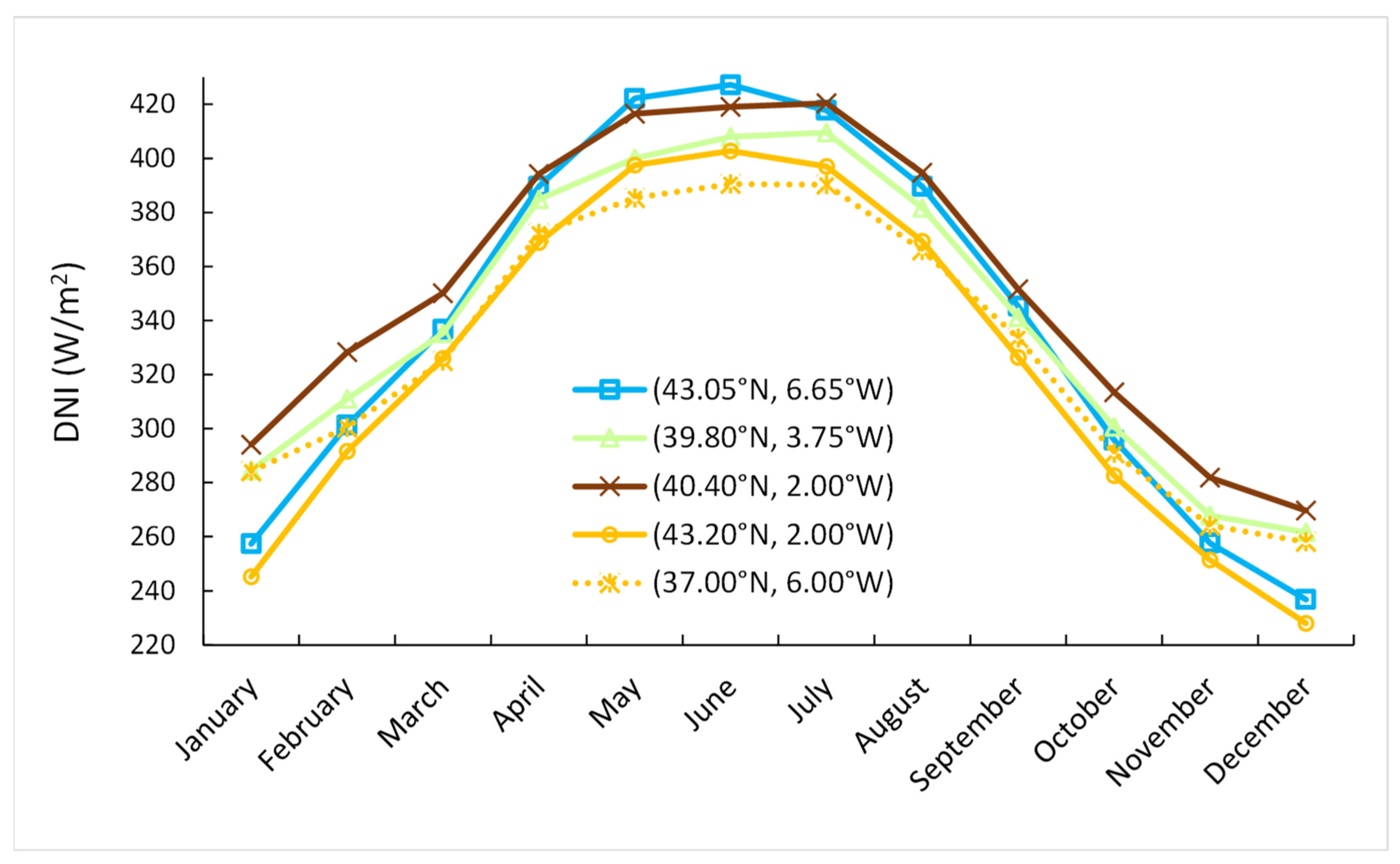
4.2. Analysis of the Selected Points

With the aim of assessing the validity of the index presented in this work, the position of five points on which we will make a more detailed study has been included in Figure 7 (white dots). The selected points cover the different clusters previously obtained, so that the analysis includes locations with different index behavior. This different behavior of suitability is the result of their different behavior in terms of the amount and variability of the radiation incident on each of them.

Table 1. Features of five selected points covering the different clusters.

Latitude	Longitude	P10	P50	IQR	SIT
43.05°N	6.65°W	251.2	341.0	127.0	0.133
39.8°N	3.75°W	266.0	338.2	99.9	0.123
40.4°N	2°W	278.2	350.8	101.8	0.071
43.2°N	2°W	240.1	326.2	116.2	0.199
37.0°N	6°W	262.3	329.3	91.2	0.166

shows the coordinates and values of the different parameters presented in the work, as well as the suitability indexes corresponding to the five selected points. To analyze these index values, Figure 8 displays the monthly evolution of incident radiation at each of the points analyzed.

The coordinate point (43.05°N, 6.65°W) is located in the northwest of the peninsula. As we can see in Figure 3, it is an area of high radiation variability, so that it has a much higher interquartile range than the rest of the selected points. Figure 8 shows that its monthly evolution is the one with the greatest variability, which has the smallest values in winter and the highest in summer, and with one of the highest 50th percentiles of the five-point group (specifically, the second largest). With these characteristics, the suitability index obtained has the third highest value (0.133), which makes this the third least suitable location for the location of the solar installation in terms of the availability of the resource.

The second point in the table (39.80°N, 3.75°W), located in the center of the peninsula, has a much smaller interquartile range than the previous point (Figure 8 also shows the enormous difference in variability between the two points), though it has a somewhat lower 50th percentile. However, despite the fact that the average radiation received at that point is slightly lower than that of the coordinates (43.05°N, 6.65°W), the enormous variability in the north makes the point (39.80°N, 3.75°W) a more suitable place for a solar installation, so that the value of its suitability index is lower than that of the first point (0.123 vs. 0.133).

As for the third point considered (40.40°N, 2.00°W), located slightly to the north and east of the previous point and over a mountainous area, the situation is opposite to the one presented above. In fact, in this case, variability is similar to that of the previous point, as shown in Figure 8 for the corresponding curves, which run practically parallel over all the months, and also shown by the corresponding interquartile ranges (101.8 W/m² and 99.9 W/m², respectively). However, the average radiation values are very different (350.8 W/m² for the latter point versus 338.2 W/m² for the location (39.80°N, 3.75°W)). This difference, therefore, confers better qualities in terms of the solar resource availability to the point (40.40°N, 2.00°W) than those corresponding to the previous point, which is reflected in the difference in suitability index values (0.071 vs. 0.123). On the other hand, according to the differences in the suitability index caused by differences in variability for the previous case, and by differences in average radiation, for this case, the suitability index is shown to be much more sensitive to changes in the 50th percentile than in variability. This result seems appropriate, since, as we have already indicated, the scarcity of radiation will always be a greater inconvenience for the installation of a solar plant than the high variability.

The fourth selected coordinates (43.20°N, 2.00°W) are those of the northernmost area. It has the lowest average radiation levels, as well as a high variability (its interquartile range is only surpassed by the first location considered), which makes it the least suitable place from those selected. This translates into the highest value of the suitability index (0.199), almost tripling the value of the most suitable point.

The four coordinates analyzed above are located in each of the four regions into which we had divided the territory based on the SIT. However, a new location (37.00°N, 6.00°W) is considered, so that the aforementioned greater sensitivity of the index to the average value as compared to variability is made more evident. So, differences between this point and (43.20°N, 2.00°W) are contrasted with differences between these two first locations considered, (43.05°N, 6.65°W) and (39.80°N, 3.75°W). With regards to points (37.00°N, 6.00°W) and (43.20°N, 2.00°W), both sites are located in the same cluster, i.e., in the region where the least suitable points are placed. The point (37.00°N, 6.00°W), located in the south of the peninsula, has a low average radiation (329.3 W/m²), a value very close to that of the northernmost point (326.2 W/m²), but it also has the least variability of the group of points, as shown in Figure 8, and in its interquartile range value. Indeed, despite this low variability (compared to the rest of the locations), the low 50th percentile makes it very unsuitable for the installation of a solar plant, which translates into a high SIT value (0.166). On the other hand, this index value is slightly lower than the 0.199 corresponding to the position (43.20°N, 2.00°W), so it is somewhat more suitable than this north point. The effect of average radiation and variability can be observed in this difference of the SIT. A difference between both points in the interquartile range—of approximately 25 W/m²—works in favor of greater suitability of the point (37.00°N, 6.00°W) along with a difference in the 50th percentile of about 3 W/m², also favorable to suitability of the point (37.00°N, 6.00°W) with regard to that of (43.20°N, 2.00°W). This yields a better suitability index in the south location by approximately 30 hundredths.

On the other hand, if we now consider these differences between the points (43.05°N, 6.65°W) and (39.80°N, 3.75°W), the results are the following: the difference between interquartile ranges is approximately 27 W/m² (similar to that of the two previously analyzed locations), which goes against the suitability of the position (43.05°N, 6.65°W) as compared to the point (39.80°N, 3.75°W), and the difference between the 50th percentile is of almost 3 W/m², which goes in favor of the suitability of that first point. Among these two positions, the first is more unfavorable to suitability, as we have already seen (0.133 vs. 0.123). Thus, the differences corresponding to the 50th percentiles and the interquartile ranges in this pair of points are practically identical to those corresponding to the pair of points (43.20°N, 2.00°W) and (37.00°N, 6.00°W), although, in one case, these differences are always favorable to the suitability of one of the positions and, in the other, one difference is favorable to suitability of a point and the other unfavorable. The significant difference in the interquartile range in support of the greater suitability of the location (39.80°N, 3.75°W) versus (43.05°N, 6.65°W) only translates into 10 hundredths of improvement in the SIT, due to the unfavorable effect caused by a small difference of 3 W/m² in the case of the 50th percentile. Nevertheless, in considering the positions (43.20°N, 2.00°W) and (37.00°N, 6.00°W), there are similar differences in the interquartile range and in the 50th percentile, but both are in favor of the point (37.00°N, 6.00°W), and translate into an improvement of the location (37.00°N, 6.00°W) as compared to (43.20°N, 2.00°W). This is in accordance with a SIT three times greater than that obtained from the point (39.80°N, 3.75°W) as compared to the point (43.05°N, 6.65°W) (30 hundredths versus 10 hundredths). Therefore, this shows the large difference in sensitivity between the SIT, the 50th percentile (which represents the amount of radiation), and the interquartile range (which represents variability).

4.3. Assessment with Storage

The new proposed index also enables the assessment of the suitability of a location, considering the chance of storing excess energy in the months in which there is a radiation surplus. In fact, following the methodology set out in Section 2, the evolution of radiation at each point throughout the year may be modified and, based on these new evolutions, the entropy and the corresponding Theil index, with the adaptations already mentioned, may be calculated.

In this sense, in Figure 9, the new suitability index is represented, considering the possibility of storage for different energy demands (expressed in terms of radiation). As in Figure 5, the values of all the points on each map are comparable, the index being obtained from the same reference value for each of these maps (the maximum value of the total radiation). Figure 9a corresponds to the case of a demand of 300 W/m². As shown, the SIT presents very low values throughout the study area, because, being a fairly low demand, the possibility of storage allows us to cover this demand in practically the entire territory throughout the year. As demand increases, this coverage decreases, as shown in the following maps, especially in the less suitable areas for the location of facilities (north of the peninsula, the Mediterranean coast, and the Ebro basin). Therefore, as demand increases, the map becomes more similar to the one represented in Figure 5, that is to say, for the case in which possibility of storage is not considered.

5. Conclusions

This study proposes a new index from the Theil index and shows that its introduction makes the assessment of the suitability of a location for installing a solar plant less arbitrary, as both availability and variability of the resource are taken into account. Indeed, a single value reflects the degree of suitability, removing the uncertainty that results from being able to choose different exceedance probabilities, besides considering the seasonal variability of radiation.

The results obtained show that the suitability index based on Theil (SIT) adequately reflects the climatic features of the study area. Then, a cluster analysis, taking the given index as a variable of interest, allows the territory to be appropriately divided into areas associated with the characteristics of the radiation. This division facilitates the final choice for the best locations in terms of the quantity and the variability of the resource for the solar installation. In this sense, the new index is clearly more sensitive to the amount of radiation, expressed in terms of the 50th percentile, than to the variability made evident from the interquartile range.

In the final analysis, satellite-based irradiance data turn out to be a powerful tool for the implementation of the index due to their wide spatial and temporal coverage. Furthermore, this index may include the effects of excess energy by storing in months when there is radiation surplus for the given demand.

References

1. World Bank Group. Solar Resource and Photovoltaic Potential of Indonesia; Energy Sector Management Assistance Program; World Bank Group: Washington, DC, USA, 2017; Available online: http://documents.worldbank.org/curated/en/729411496240730378/Solar-resource-and-photovoltaic-potential-of-Indonesia (accessed on 2 February 2024).
2. World Bank Group. Solar Resource and Photovoltaic Potential of Myanmar; Energy Sector Management Assistance Program; World Bank Group: Washington, DC, USA, 2017; Available online: http://documents.worldbank.org/curated/en/509371496240201777/Solar-resource-and-photovoltaic-power-potential-of-Myanmar (accessed on 2 February 2024).
3. Suehrcke, H.; McCormick, P. The frequency distribution of instantaneous insolation values. Sol. Energy 1988, 40, 413–422. [Google Scholar] [CrossRef]
4. Olseth, J.A.; Skartveit, A. A probability density function for daily insolation within the temperate storm belts. Sol. Energy 1984, 33, 533–542. [Google Scholar] [CrossRef]
5. Skartveit, A.; Olseth, J. The probability density and autocorrelation of short-term global and beam irradiance. Sol. Energy 1992, 49, 477–487. [Google Scholar] [CrossRef]
6. Stein, J.S.; Hansen, C.W.; Reno, M.J. The Variability Index: A New and Novel Metric for Quantifying Irradiance and PV Output Variability. In Proceedings of the World Renewable Energy Forum, Denver, CO, USA, 13–17 May 2012. [Google Scholar]
7. Peerlings, E. Cloud Gazing and Catching the Sun’s Rays: Quantifying Cloud Caused Variability, In Solar Irradiance. Master’s Thesis, Wageningen University, Wageningen, The Netherlands, 9 March 2019. [Google Scholar]
8. Dobos, A.; Gilman, P.; Kasberg, M. P50/P90 analysis for solar energy systems using the system advisor model. In Proceedings of the World Renewable Energy Forum, Denver, CO, USA, 13–17 May 2012. [Google Scholar]
9. Vindel, J.M.; Trincado, E. Discontinuity in the Production Rate Due to the Solar Resource Intermittency. J. Clean. Prod. 2021, 321, 128976. [Google Scholar] [CrossRef]
10. Ratings, F. Rating Criteria for Solar Power Projects, Utility-Scale Photovoltaic and Concentrating Solar Power. Fitch Ratings. 2011. Available online: www.fitchratings.com (accessed on 1 November 2023).
11. Vignola, F.; McMahan, A.; Grover, C. Chapter 5. Bankable solar-radiation datasets. In Solar Energy Forecasting and Resource Assessment; Elsevier: Amsterdam, The Netherlands, 2013; Volume 131, p. 97. [Google Scholar] [CrossRef]
12. Gueymard, C.; Wilcox, S.M. Spatial and temporal variability in the solar resource: Assessing the value of short-term measurements at potential solar power plant sites. In Proceedings of the Solar Conference 2009, Buffalo, NY, USA, 11–16 May 2009. [Google Scholar]
13. Fernández-Peruchena, C.M.; Gastón, M. A simple and efficient procedure for increasing the temporal resolution of global horizontal solar irradiance series. Renew. Energy 2016, 86, 375–383. [Google Scholar] [CrossRef]
14. Polo, J.; Fernández-Peruchena, C.; Salamalikis, V.; Mazorra-Aguiar, L.; Turpin, M.; Martín-Pomares, L.; Kazantzidis, A.; Blanc, P.; Remund, J. Benchmarking on improvement and site-adaptation techniques for modelled solar radiation datasets. Sol. Energy 2020, 201, 469–479. [Google Scholar] [CrossRef]
15. Fernández-Peruchena, C.M.; Polo, J.; Martín, L.; Mazorra, L. Site-Adaptation of modelled solar radiation data: The site adapt procedure. Remote Sens. 2020, 12, 2127. [Google Scholar] [CrossRef]
16. Hoyer-Klick, C.; Beyer, H.G.; Dumortier, D.; Schroedter Homscheidt, M.; Wald, L.; Martinoli, M.; Schillings, C.; Gschwind, B.; Menard, L.; Gaboardi, E.; et al. MESoR e management and exploitation of solar resource knowledge. In Proceedings of the solarPACES, Berlin, Germany, 15–18 September 2009. [Google Scholar]
17. Vignola, F.; Harlan, P.; Perez, R.; Kmiecik, M. Analysis of satellite derived beam and global solar radiation data. Sol. Energy 2007, 81, 768–772. [Google Scholar] [CrossRef]
18. Zelenka, A.; Perez, R.; Seals, R.; Renne, D. Effective accuracy of satellite-derived hourly irradiances. Theor. Appl. Climatol. 1999, 62, 199–207. [Google Scholar] [CrossRef]
19. Cano, D.; Monget, J.M.; Aubuisson, M.; Guillard, H.; Regas, N.; Wald, L. A method for the determination of the global solar radiation from meteorological satellite data. Sol. Energy 1986, 37, 631–639. [Google Scholar] [CrossRef]
20. Moser, W.; Raschke, E. Mapping of global radiation and of cloudiness from METEOSAT image data. Theory and ground truth comparisons. Meteorol. Rundsch. 1983, 36, 33–41. [Google Scholar]
21. Gautier, C.; Diak, G.; Masse, S. A simple physical model to estimate incident solar radiation at the surface from GOES satellite data. J. Appl. Meteorol. 1980, 19, 1005–1012. [Google Scholar] [CrossRef]
22. Yuzer, E.O.; Bozkurt, A. Deep learning model for regional solar radiation estimation using satellite images. Ain Shams Eng. J. 2003, 14, 10205. [Google Scholar] [CrossRef]
23. López, M.; Aler, R.; Galván, I.M.; Rodríguez, F.J.; Pozo, A.D. Improving Solar Radiation Nowcasts by Blending Data-Driven, Satellite-Images-Based and All-Sky-Imagers-Based Models Using Machine Learning Techniques. Remote Sens. 2003, 15, 2328. [Google Scholar] [CrossRef]
24. Verbois, H.; Saint-Drenan, Y.-M.; Libois, Q.; Michel, Y.; Cassas, M.; Dubus, L.; Blanc, P. Improvement of satellite-derived surface solar irradiance estimations using spatio-temporal extrapolation with statistical learning. Sol. Energy 2023, 258, 175–193. [Google Scholar] [CrossRef]
25. Oliveti, G.; Arcuri, N.; Ruffolo, S. Effect of climatic variability on the performance of solar plants with interseasonal storage. Renew. Energy 2000, 19, 235–241. [Google Scholar] [CrossRef]
26. Dohse, K.; Jürgens, U.; Nialsch, T. From “fordism” to “toyotism”? The social organization of the labor process in the Japanese automobile Industry. J. Politics Soc. 1985, 14, 115–146. [Google Scholar] [CrossRef]
27. Bischoff, M.; Jahn, J. Economic objectives, uncertainties and decision making in the energy sector. J. Bus. Econ. 2016, 86, 85–102. [Google Scholar] [CrossRef]
28. Harrouni, S.; Guessoum, A. Using fractal dimension to quantify long-range persistence in global solar radiation. Chaos Solit. Fractals 2009, 41, 1520–1530. [Google Scholar] [CrossRef]
29. Bertok, B.; Bartos, A. Renewable energy storage and distribution scheduling for microgrids by exploiting recent developments in process network synthesis. J. Clean. Prod. 2020, 244, 118520. [Google Scholar] [CrossRef]
30. Strongin, S.; Eugeni, F. The Cost of Uncertainty. Chic. Fed. Lett. 1991, 43, 1. Available online: https://login.bucm.idm.oclc.org/login?url=https://www-proquest-com.bucm.idm.oclc.org/docview/214569638?accountid=14514 (accessed on 2 February 2024).
31. Libra, M.; Mrázek, D.; Tyukhov, I.; Severová, L.; Poulek, V.; Mach, J.; Šubrt, T.; Beránek, V.; Svoboda, R.; Sedláček, J. Reduced real lifetime of PV panels—Economic consequences. Sol. Energy 2023, 259, 229–234. [Google Scholar] [CrossRef]
32. Dong, S.; Kremers, E.; Brucoli, M.; Rothman, R.; Brow, S. Improving the feasibility of household and community energy storage: A techno-enviro-economic study for the UK. Renew. Sustain. Energy Rev. 2020, 131, 110009. [Google Scholar] [CrossRef]
33. Olczak, P.; Żelazna, A.; Stecuła, K.; Matuszewska, D.; Lelek, Ł. Environmental and economic analyses of different size photovoltaic installation in Poland. Energy Sustain. Dev. 2022, 70, 160–169. [Google Scholar] [CrossRef]
34. Markowitz, H. Portfolio Selection: Efficient Diversification of Investments; Blackwell: Malden, MA, USA, 1991. [Google Scholar]
35. Pfeifroth, U.; Kothe, S.; Müller, R.; Trentmann, J.; Hollmann, R.; Fuchs, P.; Werscheck, M. Surface Radiation Data Set—Heliosat (SARAH)—Edition 2, Satellite Application Facility on Climate Monitoring. 2017. Available online: https://wui.cmsaf.eu/safira/action/viewDoiDetails?acronym=SARAH_V002 (accessed on 1 March 2023).
36. CM-SAF. Validation Report Meteosat Solar Surface Radiation and Effective Cloud Albedo Climate Data Record SARAH-2. 2016. Available online: https://www.cmsaf.eu/SharedDocs/Literatur/document/2016/saf_cm_dwd_val_meteosat_hel_2_1_pdf.html (accessed on 1 March 2023).
37. CM-SAF. Algorithm Theoretical Baseline Document Meteosat Solar Surface Radiation and Effective Cloud Albedo Climate Data Records—Heliosat SARAH-2. 2017. Available online: https://wui.cmsaf.eu/safira/action/viewProduktSearch (accessed on 1 March 2023).
38. Levy, J. Radical Uncertainty. Crit. Q. 2020, 62, 15–28. [Google Scholar] [CrossRef]
39. Robicheck, A.A.N.; Myers, S.C. Conceptual problems in the use of risk-adjusted discount rates. J. Financ. 1996, 21, 727–730. [Google Scholar] [CrossRef]
40. Copeland, D.E.; Weston, J.F. Financial Theory and Corporate Policy; Addison Wesley: Boston, MA, USA, 1983. [Google Scholar]
41. Altimir, O.; Crivelli, A.; Piñera, S. Análisis de Descomposición. Una Generalización del Método de Theil, Development Research Center del Banco Mundial and Comisión Económica para América Latina. 1977. Available online: https://hdl.handle.net/11362/32365 (accessed on 2 February 2024).
42. Gini, C. On the Measure of Concentration with Special Reference to Income and Statistics; General Series; Colorado College Publication: Denver, CO, USA, 1936; Volume 208, pp. 73–79. [Google Scholar]
43. Theil, H. Statistical Decomposition Analysis: With Applications in the Social and Administrative Sciences, Studies in Mathematical and Managerial Economics; North-Holland Publishing: Amsterdam, The Netherlands, 1972; Volume 14. [Google Scholar]
44. Theil, H. More on Log-Change Index Numbers. Rev. Econ. Stat. 1974, 56, 552–554. [Google Scholar] [CrossRef]
45. Rohde, N. Lorenz Curves and Generalised Entropy Inequality Measures. In Modeling Income Distributions and Lorenz Curves, Economic Studies in Equality, Social Exclusion and Well-Being; Chotikapanich, D., Ed.; Springer: New York, NY, USA, 2008; Volume 5, pp. 271–283. [Google Scholar]
46. Shorrocks, A.F. The Class of Additively Decomposable Inequality Measures. Econometrica 1980, 48, 613–625. [Google Scholar] [CrossRef]
47. Theil, H. Economics and Information Theory; North-Holland Pub. Co: Amsterdam, The Netherlands, 1967. [Google Scholar]
48. Jin, X.; Han, J. K-Means Clustering. In Encyclopedia of Machine Learning; Sammut, C., Webb, G.I., Eds.; Springer: Boston, MA, USA, 2011. [Google Scholar] [CrossRef]
49. Davies, D.L.; Bouldin, D.W. A cluster separation measure. IEEE Trans. Pattern Anal. Mach. Intell. 1979, PAMI-1, 224–227. [Google Scholar] [CrossRef]
50. Rousseeuw, P.J. Silhouettes: A graphical aid to the interpretation and validation of cluster analysis. J. Comput. Appl. Math 1987, 20, 53–65. [Google Scholar] [CrossRef]
51. Walsh, M.; de la Torre, D.; Shapouri, H.; Slinksky, S. Bioenergy crop production in the United States. Environ. Resour. Econ. 2003, 24, 313–333. [Google Scholar] [CrossRef]
52. Lankoski, J.; Ollikainen, M. Bioenergy Crop Production and Climate Policies: A von Thunen Model and the Case of Reed Canary Grass in Finland. Eur. Rev. Agric. Econ. 2008, 35, 519–546. [Google Scholar] [CrossRef]
53. Von Thünen, J. The Isolated State in Relation to Agriculture and Political Economy; Palgrave Macmillan: London, UK, 2009. [Google Scholar]
Figure 1. Physical map of the Iberian Peninsula. Source: Nations Online Project. https://www.nationsonline.org/oneworld/map/Iberian-Peninsula-topographic-map.htm (accessed on 2 February 2024).
Remotesensing 16 01039 g001
Figure 2. Radiation percentiles associated with the exceedance probabilities of: (a) 90%; (b) 50%.
Remotesensing 16 01039 g002
Figure 3. Interquartile range.
Remotesensing 16 01039 g003
Figure 4. Average versus variance of the DNI (in W/m2) throughout the study territory.
Remotesensing 16 01039 g004
Figure 5. Map of the suitability index based on Theil (SIT).
Remotesensing 16 01039 g005
Figure 6. Optimal number of clusters: (a) Davis–Bouldin method; (b) silhouette method.
Remotesensing 16 01039 g006
Figure 7. Division of the territory into clusters with similar behavior to the SIT.
Remotesensing 16 01039 g007
Figure 8. Monthly evolution of the DNI in the five sites.
Remotesensing 16 01039 g008
Figure 9. SIT for different demands after storage: (a) 300 W/m2; (b) 350 W/m2; (c) 400 W/m2; (d) 450 W/m2.
Remotesensing 16 01039 g009