Article

Landsat 9 Thermal Infrared Sensor-2 (TIRS-2) Pre- and Post-Launch Spatial Response Performance

1
Digital Imaging and Remote Sensing Laboratory (DIRS), Rochester Institute of Technology, 54 Lomb Memorial Drive, Rochester, NY 14623, USA
2
Science Systems and Applications, Inc., 10210 Greenbelt Rd, Lanham, MD 20706, USA
3
NASA Goddard Space Flight Center, Greenbelt, MD 20771, USA
*
Author to whom correspondence should be addressed.
Remote Sens. 2024, 16(6), 1065; https://doi.org/10.3390/rs16061065
Submission received: 9 February 2024 / Revised: 8 March 2024 / Accepted: 9 March 2024 / Published: 18 March 2024

Abstract

:
The launch of Landsat 9 (L9) on 27 September 2021 marks the ongoing commitment of the Landsat mission to delivering users with calibrated Earth observations for fifty years. The two imaging sensors on L9 are the Thermal Infrared Sensor-2 (TIRS-2) and the Operational Land Imager-2 (OLI-2). Shortly after launch, the image data from OLI-2 and TIRS-2 were evaluated for both radiometric and geometric quality. This paper provides a synopsis of the evaluation of the spatial response of the TIRS-2 instrument. The assessment focuses on determining the instrument’s ability to detect a perfect knife edge. The spatial response was evaluated both pre- and post-launch. Pre-launch testing was performed at NASA Goddard Space Flight Center (GSFC) under flight-like thermal vacuum (TVAC) conditions. On orbit, coastline targets were identified to evaluate the spatial response and compared against Landsat 8 (L8). The pre-launch results indicate that the spatial response of the TIRS-2 sensor is consistent with its predecessor on board L8, with no noticeable decline in image quality to compromise any TIRS science objectives. Similarly, the post-launch analysis shows no apparent degradation of the TIRS-2 focus during the launch and the initial operational timeframe.

1. Introduction

The launch of Landsat 9 (L9), on 27 September 2021, furthers the Landsat mission’s objective to provide high-quality Earth observation data to the scientific community [1,2,3]. The inclusion of the Thermal Infrared Sensor-2 (TIRS-2) instrument continues the thermal observation of the Earth’s surface as part of the L9 mission. As with all Landsat missions, image data from TIRS-2 are assessed for radiometric and geometric quality. One of the important geometric assessment parameters is the spatial response of the instrument, which involves determining how well the instrument detects a perfect edge in a scene [4]. The spatial response provides users with a metric to describe the optical sharpness of an image and how well that metric compares to previous Landsat data [5,6].
TIRS-2 is a near copy of the TIRS-1 instrument on board Landsat 8 (L8) with several improvements in electronic redundancy and stray light mitigation [7,8]. The instrument acquires Earth image data in a push-broom configuration in two spectral channels centered at 10.8 μ m (band 10) and 12.0 μ m (band 11) in wavelength. TIRS-2 contains a four-element refractive telescope that focuses light onto the focal plane containing three detector arrays. Spectral filters are placed over the detector arrays to produce the two spectral channels. The across-track field-of-view is ±7.5 degrees, which spans a 185 km swath width on the ground. Each detector element produces a Ground Sampling Distance (GSD) of approximately 100 m for each spectral band. In the final Landsat product released by the U.S. Geological Survey (USGS), TIRS-2 image data are resampled and geo-located to 30 m pixels to be consistent with Visible Near-Infrared (VNIR) and Short-Wave Infrared (SWIR) imagery data collected by the other instrument on L9, the Operational Land Imager-2 (OLI-2). The dual-channel design of the TIRS sensor offers the capability to retrieve surface temperature (ST) using the split-window algorithm [9]. Surface temperature data from space-borne sensors are crucial for monitoring fires, lava flows, as well as drought and vegetation stress [10]. The ST product from Landsat is also a crucial component of the models integrated in openET for calculating surface energy balances to assess water use and managing water rights [11]. Ideally, these assessments should be performed at fine resolutions of individual agricultural fields. Hence, the spatial resolution remains a key limiting factor in most applications of space-borne thermal sensors. As a result, a thorough assessment of the spatial performance is crucial.
The spatial response of TIRS-2 was first assessed in pre-launch testing at NASA Goddard Space Flight Center (GSFC) under flight-like thermal vacuum (TVAC) conditions. The response to a knife-edge target was determined for samples of detector elements spanning the across-track field-of-view (FOV). The spatial response was again assessed post-launch using Earth features. The critical portion of the post-launch geometric characterization of the sensor occurs during the commissioning period of the satellite, which is followed by the on-orbit activation of the instrument and nominal operational settings [2]. The sensors on board the spacecraft can be impacted due to vibrations during launch, the transition from a 1-G to a 0-G environment, and due to any adjustments of the on-orbit thermal environment [2]. The post-launch characterization ensures that the optical system did not shift during launch, thereby affecting image quality and still meeting its mission level requirements or specifications. This paper documents the efforts to characterize the spatial performance of the TIRS-2 instrument by discussing the theoretical methods of assessment, describing the test set-up and procedures, and presenting the results and comparing them to the previous L8 TIRS-1 instrument’s performance.

2. Methodologies

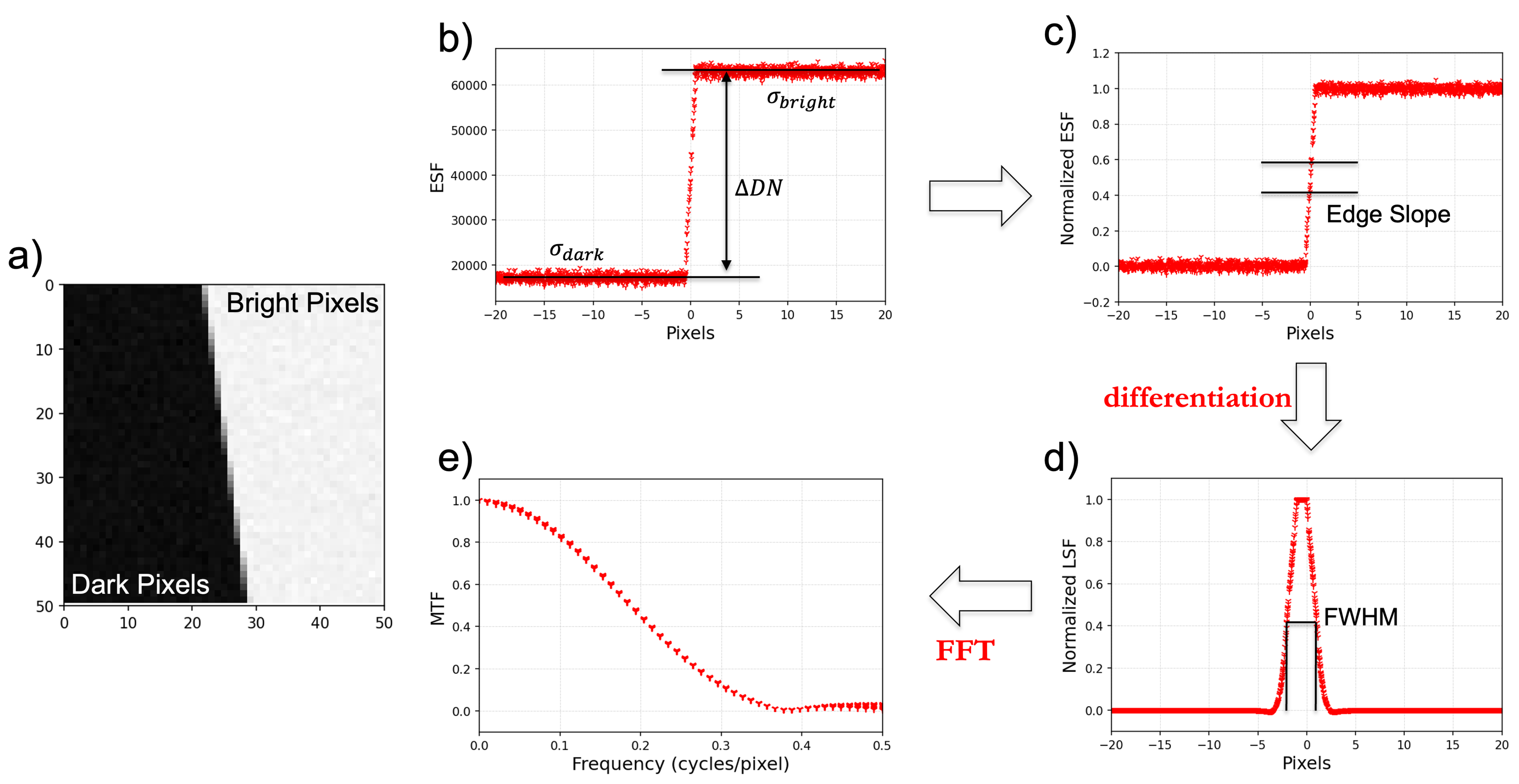
2.1. Theoretical Development

The spatial quality of an optical remote sensing instrument is closely related to the the GSD and the instantaneous field-of-view (IFOV) defined by the pixel size and focal length [12]. However, a more accurate representation of the spatial resolution, and in-turn, the geo-spatial quality of the sensor, should also consider the point spread function (PSF) and modulation transfer function (MTF) of the system [12]. The PSF, in the spatial domain, and the MTF, in the frequency domain, are good measures of the image quality or sharpness of linear, shift-invariant imaging systems [12,13,14]. The images obtained by optical sensors are represented by the convolution of the imaging system’s response, the PSF, and the object target [12,13]. The PSF of most linear, shift-invariant imaging systems is mathematically a spatial convolution of the different optical and detector components, as well as any effects due to the motion and electronics [13].
The ISO 12233 standard [15,16], which is also known as the slanted-edge method, is used in this work to determine the spatial characteristics of the TIRS-2 sensor both during pre- and post-launch. The edge spread function (ESF) is the system response to a slanted edge oriented in either the across- and along-direction of the sensor and is a representation of the one-dimensional integration of the PSF [5].
The construction of the ESF, using the ISO 12233 standard, for a slanted target is graphically represented in Figure 1 [17]. The first step involves identifying the edge within the image (1). A line is then built perpendicular to the edge (2). Each point or pixel (3) along the edge is projected onto the perpendicular line (4). This process is repeated for each row of the image data. The edge is sampled in a manner to allow sub-pixel reconstruction with respect to the sample grid. This results in a highly accurate estimation of an over-sampled edge spread function (5) of the system [17]. The line spread function (LSF), which is the system response to a high contrast line, is determined by the derivative of the ESF, while the Fourier Transform of the normalized LSF produces a one-dimensional slice of the MTF [17].

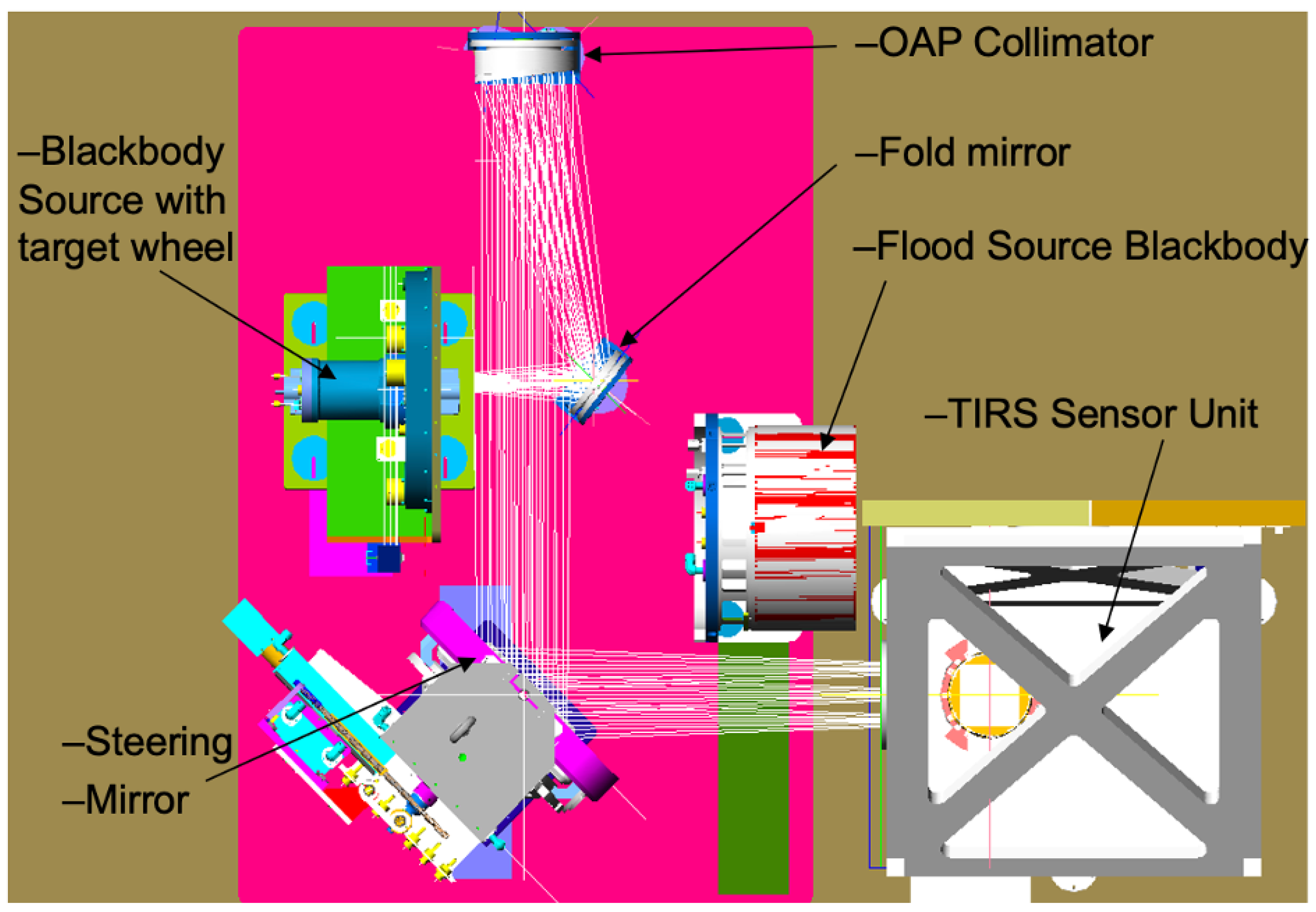
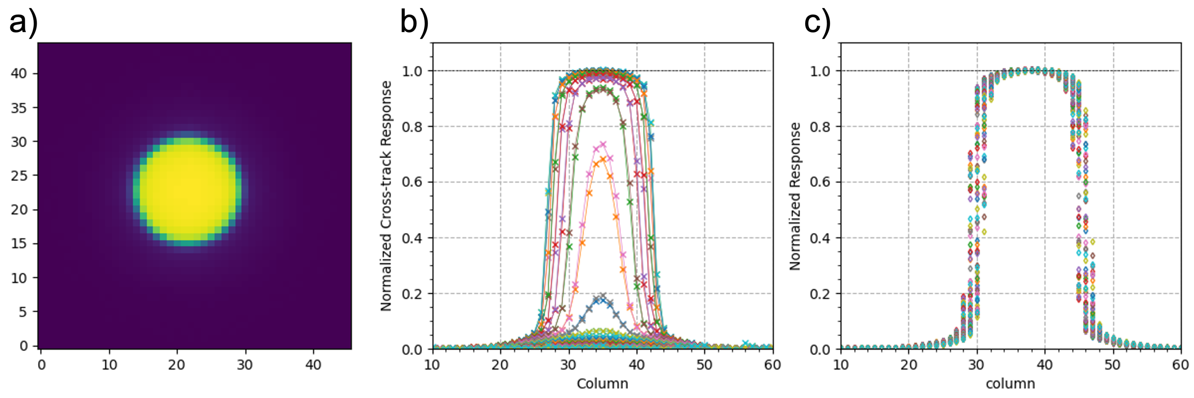
2.2. Pre-Launch Analysis

In this section, we detail the lab geometric characterization and calibration of the TIRS-2 sensor at the NASA GSFC facilities. The lab testing was performed in the GSFC thermal vacuum chamber (TVAC) to simulate the expected on-orbit environment of the instrument. The lab protocol to measure the spatial response of the TIRS-2 system is similar to the work detailed by Wenny et al. (2015) for L8 [5,18]. The TIRS-2 TVAC calibration used the same custom-built Calibration Ground Support Equipment (CGSE) system developed for the TIRS-1 sensor [8,19,20]. A schematic layout of the CGSE and TIRS-2 is shown in Figure 2. The CGSE system consists of a NIST traceable blackbody and a motorized filter wheel with numerous target-aperture shapes. The CGSE blackbody source was re-calibrated by Space Dynamics Laboratory (North Logan, UT) immediately prior to beginning the TVAC testing. The TVAC testing was conducted in three stages. During the first segment, TIRS-2 Imaging Performance and Cryoshell Evaluation (TIPCE) were primarily used to collect measurements to verify the mitigation of stray light, which was observed in TIRS-1 on L8, by the installation of mechanical baffles [8,21,22]. The stray-light-mitigation procedure for TIRS-2 is further detailed by Montanaro et al. (2022) [8]. The second (TVAC1) and third (TVAC2) segments included sets of data collections at a series of temperature plateaus to simulate the expected range of operational environments on orbit. These two segments were separated by the vibrational and electro-magnetic interference (EMI) testing. Data sets to assess the spatial characterization of TIRS-2 were collected during all three periods; however, only the TVAC1 and TVAC2 data were used for spatial requirement verification. The lab geometric characterization used the blackbody source with the target wheel and employed the steering mirror to point the edge target onto the desired location of the focal plane array (FPA). Figure 3 shows the CGSE mounted in the TVAC chamber.
For the spatial characterization, the blackbody was set to 300-K, and the target shapes used in the analysis were blank targets (for background correction): a 90 by 90 pixel square target (for flat-fielding) and a circular target with a 16-pixel diameter (the primary edge target). This approach was used successfully for TIRS-1 after it was determined that the extended knife-edge target typically used for spatial analysis had vignetting issues.
The test measurement procedure consisted of collecting multiple image frames of the circular target as it is moved in incremental sub-pixel (1/5) steps in both across-/along-track directions over 3 pixels. Figure 4a shows an example image of the circular target. The measurement was repeated for several locations in the across-track FOV (the three detector arrays) of the instrument and each band. The first step in determining the edge response involves performing a background correction and flat-fielding of the data collected. The background correction is performed by imaging multiple frames of the blank target and taking the average. Each frame of the circular target is subtracted by the average background image. The flat-fielding, which removes any pixel-to-pixel variations, is performed by taking multiple images of the square target and correcting for the background, similar to the circular target. Each frame of the background-corrected circular target is then divided by the average of all background-corrected square target frames.
Figure 4b shows all cross-section data of a background-corrected, flat-fielded circle image in the across-track direction, which has been normalized to the maximum value. The 80 maximum frames collected during the incremental sub-pixel (1/5) steps in the across-track direction are shown in Figure 4c. The edge response for each frame is then determined by fitting the data to a Fermi function [5,18,23]:
f ( x ) = d + a 1 + e ( x b ) / c
where d is the bias level, a is a scaling factor, b is the inflection point in the curve, and c represents the sharpness of the edge. The Fermi function is used to measure the subpixel edge location of the profile and shift the data to a common pixel reference, shown in Figure 5a. The shifted edge response is linearly interpolated to uniform pixel spacing (0.01 pixels), and the edge response/extent is determined. The left edge of the response is shown in Figure 5b. The LSF is obtained by first-order differentiation of the edge spread function. The MTF of the system is also calculated by applying a Fast Fourier Transformation to the LSF and normalizing by the value at the zeroth frequency (Figure 5c). This process is repeated for all the data collected in the across-/along-track direction and for each TIRS-2 band.
As per the TIRS-2 instrument requirement documentation, the edge slope is defined as the rate of increase in intensity from the 0.4 to 0.6 amplitude levels of the ESF, while the edge extent is the distance between the 0.1 and 0.9 amplitude levels of the ESF [5] (this is highlighted in Figure 5b). The TIRS-2 spatial requirement sets the edge slope to be greater than 0.47 and the edge extent to be less than 240 m for a 100 m TIRS-2 pixel. The TIRS-2 instrument edge slope and edge extent and the MTF value at Nyquist during the pre-launch lab characterization is reported.

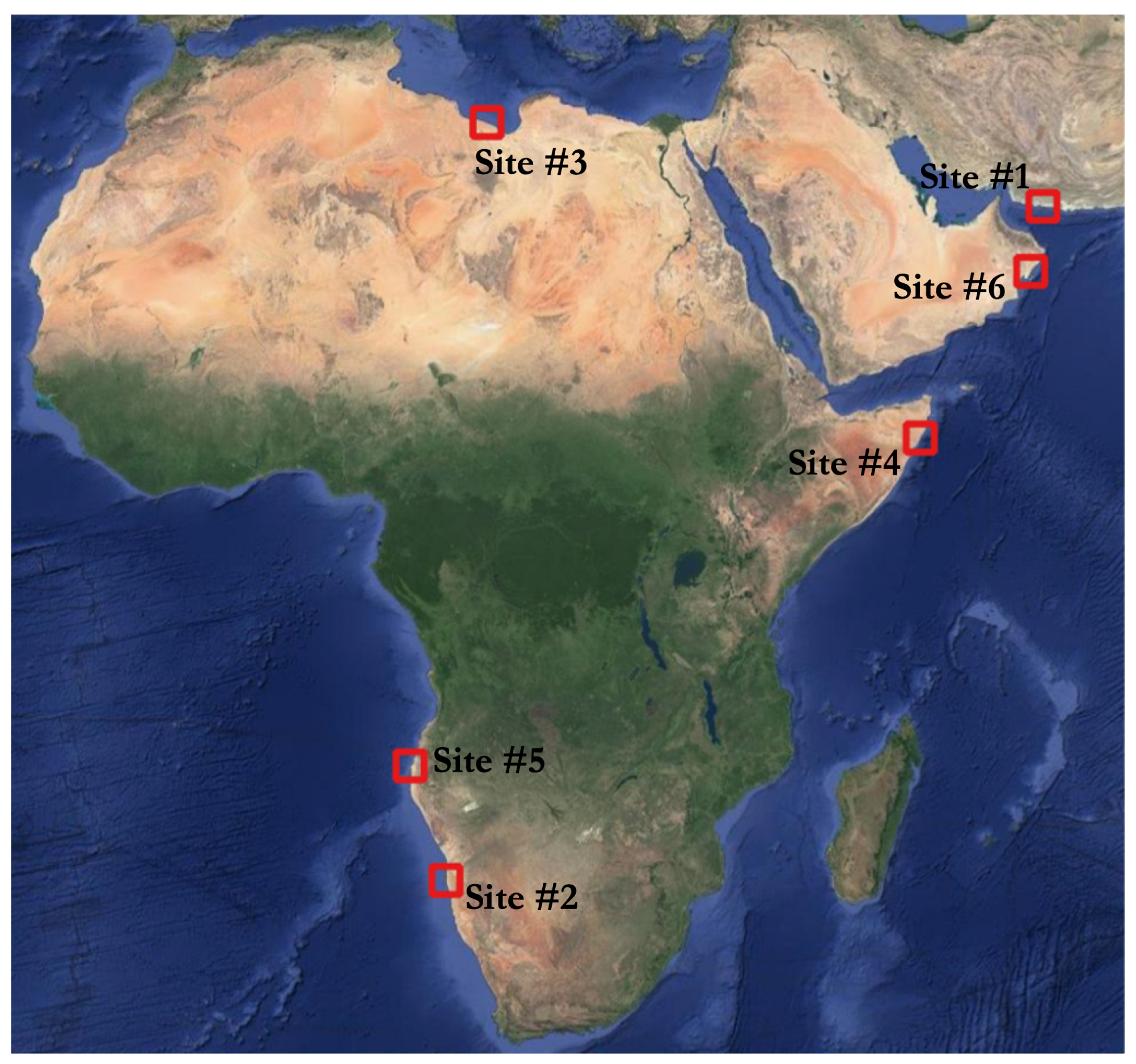
2.3. Post-Launch Analysis

The methodology to derive the PSF/MTF for the post-launch analysis is also similar to what was published by Wenny et al. (2015) for L8 [5,18]. This implementation requires the edge target to be at a proper orientation with respect to the orbit of the satellite. If not at the correct orientation, the edge data are non-uniformly distributed, i.e., data points along the edge are clustered together, which leads to poor estimations of the PSF/MTF [12]. The ideal edge target should be between 6 and 8 degrees with respect to the sampling grid of the instrument detectors [12]. The edge target also needs to span a sufficient number of rows/columns of the image for enough pixels to over-sample the edge for accurate reconstruction.
The workflow to perform the spatial analysis is shown in Figure 6 for a sinc function with random Gaussian noise added at an angle of 8 degrees. The first step is developing the over-sampled ESF by fitting the data to a modified Fermi function [5,18]:
f ( x ) = d + b d 1 + e s ( x e ) + g x
where x represents the pixel location for row f, d and b are the magnitudes for the dark and bright side of the edge, respectively, e is the edge location, and s represents the steepness of the edge. The Fermi function was modified by adding the linear term “gx” [5,18]. The term was added due to the non-uniformity associated with naturally occurring edge targets from satellite-borne systems. This modified Fermi function was fit to the data using an optimization algorithm, such as the Levenberg–Marquardt algorithm, to solve for the output parameters. The edge profiles are aligned based on the location of the edge to estimate the edge spread function. The ESF is normalized by subtracting the linear term of the modified Fermi function and normalized by dividing the height of the edge (b − d) [5]. The ESF is also simultaneously filtered, reducing high-frequency noises, by using a low-pass filter (Savitzky–Golay [24]). This outputs a uniformly over-sampled ESF, which has had any high-frequency noises removed, without significantly impacting any frequencies below Nyquist [12]. The LSF is obtained by first-order differentiation of the edge spread function. The final step is calculating the MTF of the system by applying a Fast Fourier Transformation to the LSF and normalizing by the value at the zeroth frequency.
The signal-to-noise ratio (SNR) is measured to evaluate the accuracy of the PSF/MTF estimations, which is defined as
S N R = Δ D N ( σ b r i g h t + σ d a r k ) / 2
where ΔDN is the edge height of the ESF and σ b r i g h t and σ d a r k are the averages of the standard deviation of the bright and dark side of the edge, respectively. In previous work, modeling has shown SNR > 50 produces accurate estimations of the PSF/MTF [5,12].
The development of a man-made target for TIRS-2 on-orbit ESF estimation is impractical due to the large IFOV of the Landsat thermal sensor. As a result, naturally occurring thermal edge targets were identified, specifically shorelines with high thermal contrast, to study the spatial performance of TIRS-2 on orbit. These sites were chosen based on various criteria described in detail by Wenny et al. (2015). The optimal naturally occurring edge target sites should be thermally uniform over both land and water and have a high thermal contrast (significant difference in temperature) between the land and water, a physically stable shoreline (minimal change over time and impact from tides) with a sharp transition between land and water, and a proper orientation with respect to the orbit of L8/L9 [5].
The focus of the optical system can be altered by changing the temperature of the telescope lenses [25]. During ground testing, the telescope temperature was set to its operational value of approximately 190 K and the distance between the telescope and the focal plane was fixed to put the detector arrays at the optimal focus position. During L9 commissioning, a characterization test was performed to purposely de-focus and re-focus the telescope system by acquiring image data at lens temperatures of ±4 K from the nominal value. The focusing test scheduled during the commissioning phase is detailed in Table 1.
Ultimately, the site-choosing criteria detailed by Wenny et al. (2015) [5], in conjunction with the orbit of L9 during the focusing test, were utilized to select six different sites to study the spatial performance of TIRS-2 post-launch. These naturally occurring edge target sites primarily consist of coastlines in the Middle East and Africa, where a significant thermal contrast exists between the cold ocean and the warm desert [5]. A target detection algorithm [26] was implemented to find shoreline edges for several L9 scenes over this region. Landsat is in a polar orbit with an inclination of 98°, and shorelines with an orientation as close as possible to 8 ± 8° from the cross-/along-track direction of the satellite were chosen for the analysis. For each pixel along the shoreline edge, we measured the SNR of the ESF and the Full-Width at Half-Maximum (FWHM) from the LSF. Pixels with a high SNR (showing high thermal contrast between land and water) and a low standard deviation of the FWHM (representing physically stable shorelines and sharp transitions between land/water) were chosen as “ideal” edge targets. This resulted in six optimal target sites to perform the spatial analysis. These sites are shown in Figure 7 and detailed in Table 2.
For the focusing test, the L9 TIRS-2’s spatial performance was compared against L8 TIRS-1 over the same site. Note that we tried to find the nearest L8 data to L9, i.e., they were not temporally coincidental. We also monitored how the spatial quality of these sites changed over time from November 2021 to April 2023. The analysis was performed on the standard L1T product released by USGS for each TIRS-2 band. The TIRS-2 has a GSD of 100 m, which is resampled to 30 m in the L1T product. A 50 by 50 pixel ROI image of the edge target was chosen to perform the analysis. We report the edge slope, FWHM, and MTF value at Nyquist for each edge target site.

3. Results and Discussion

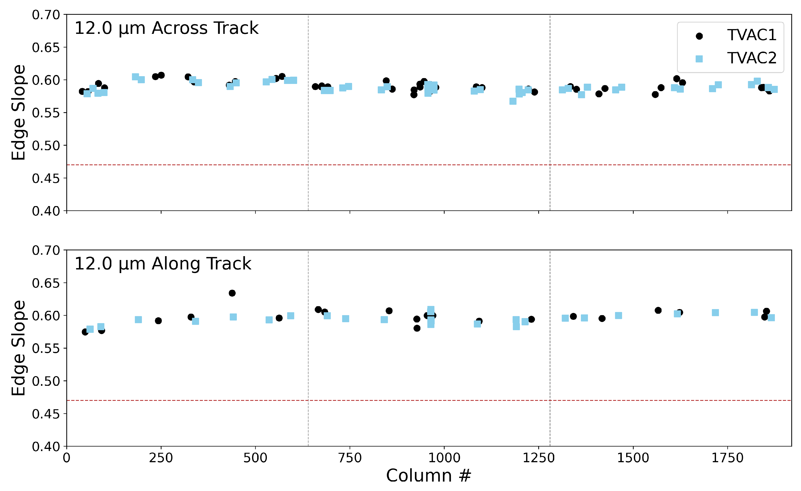
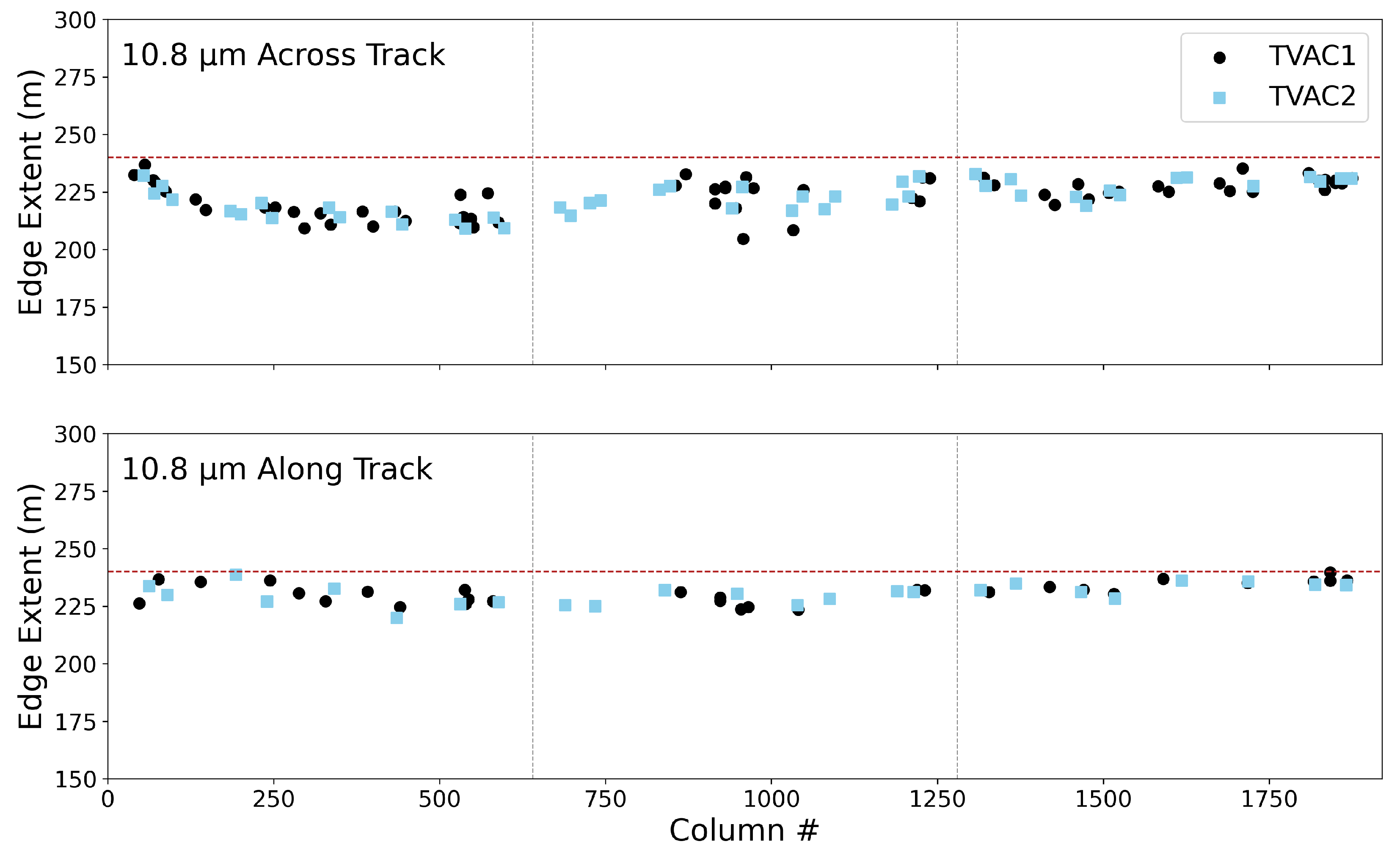
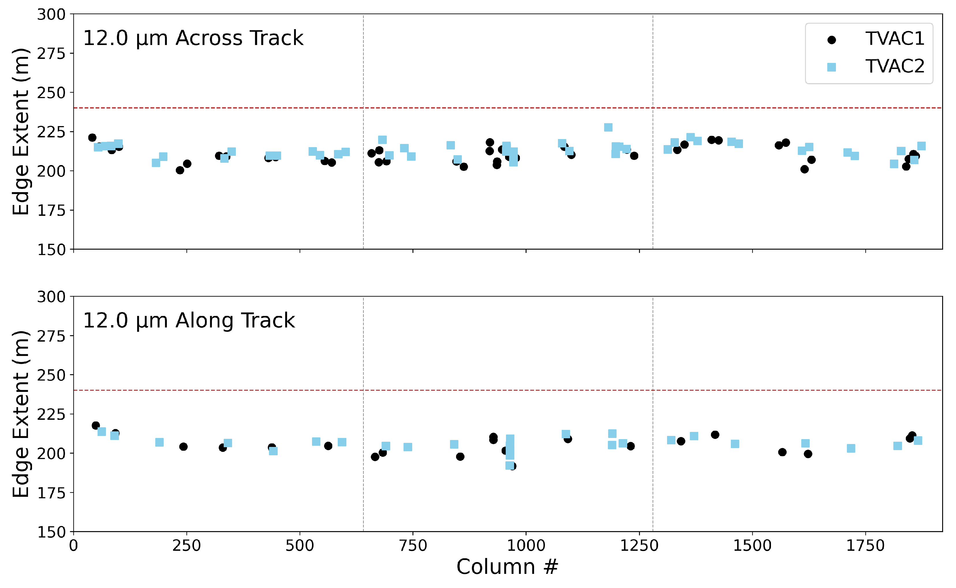
3.1. Pre-Launch Analysis

The spatial characterization data were collected during all three segments of TVAC. Over 150 data sets were collected covering locations across the full FOV for both TIRS-2 bands. The data collections occurred for every operational environmental thermal plateau during TVAC. Data at several of the locations in the FOV were collected multiple times at slightly different CGSE configurations to verify the repeatability of the measurement protocol. The data collected during the TIPCE TVAC segment were at the telescope–FPA assembly level and provided an initial assessment of the spatial performance. Only data collected at the full instrument level during TVAC1 and TVAC2 were used for spatial performance requirement verification.
The edge analysis was performed in both the across- and along-track directions. In order to have sufficient numbers of pixels on the dark side of the edge, the initial placement of the target image allowed only one edge to be analyzed in the along-track direction. For the across-track analysis, the edges on both sides of the circular target were available for analysis, effectively doubling the number of measurements. The lessons learned during the TIRS-1 pre-launch analysis indicated that it was not necessary to try to sample repeatedly at the same locations during each TVAC plateau. For TIRS-2, a more random set of locations across each band and SCA was selected, which allowed for a more thorough sampling across the complete FOV than what was performed for TIRS-1 when combining the results from TVAC1 and TVAC2.
The TIRS spatial requirements were written in terms of the edge slope and extent and their uniformity across the FOV, so this was the primary analysis performed during pre-launch. Figure 8 shows the overall results for the edge slope for band 10 in the across- and along-track directions. Figure 9 shows similar derived edge slopes for band 11. Both data collected during TVAC1 and TVAC2 are displayed. It is evident that the edge slopes all exceeded 0.55 across the whole FOV, which are well above the requirement of 0.47. Band 11 has marginally higher edge slopes than band 10, which is consistent with analysis performed on TIRS-1 [5]. The other noticeable feature is the slight “frown” where the edge slopes are lower at the extreme ends of the FOV. This behavior is not unexpected as the telescope focus is optimized for the center of the FOV. Figure 10 and Figure 11 display the results for the edge extent analysis for both bands and along- and across-track. As with the edge slopes, the spatial requirement is met across the full FOV, with the performance in band 11 slightly better than that of band 10. The edge slope and extent results are consistent between TVAC1 and TVAC2, providing confidence that the instrument did not suffer any detrimental effects during vibration testing.
An overall summary of the key spatial analysis metrics during the pre-launch analysis for TIRS-2 is detailed in Table 3. Similar values for TIRS-1 are included for comparison. The values presented are the mean and standard deviation for all points across the FOV in a given band and track direction. The mean edge slopes for TIRS-2 agree well with those of TIRS-1, with slightly better performance in band 11. The edge extents also show consistent behavior between TIRS-2 and TIRS-1. Again, band 11’s edge extent performance is better than that of band 10 for both instruments. The standard deviations for TIRS-1 are larger primarily due to a much lower number of data points collected. The MTF at Nyquist frequency is also included for TIRS-2, while Figure 5c shows an example of the normalized edge response and MTF measured in TVAC. The MTF analysis was not included as part of the requirement verification at pre-launch, but is included here for comparison with the on-orbit-derived MTF.

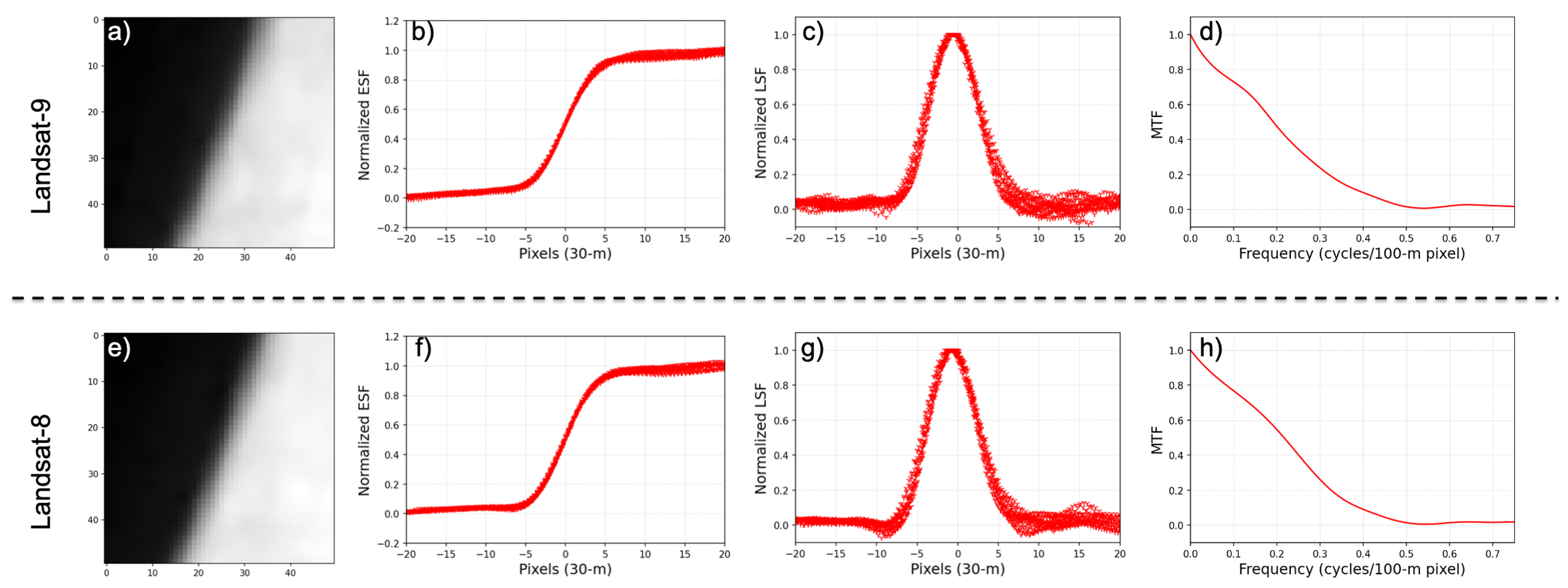
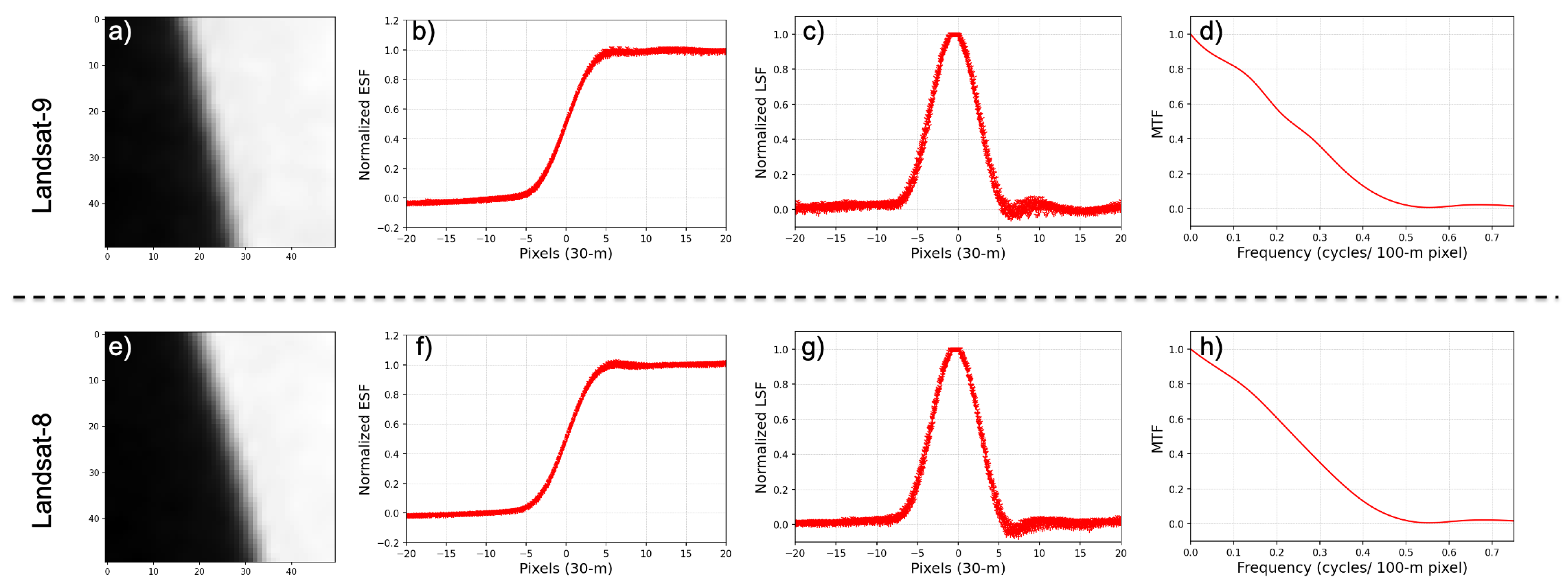
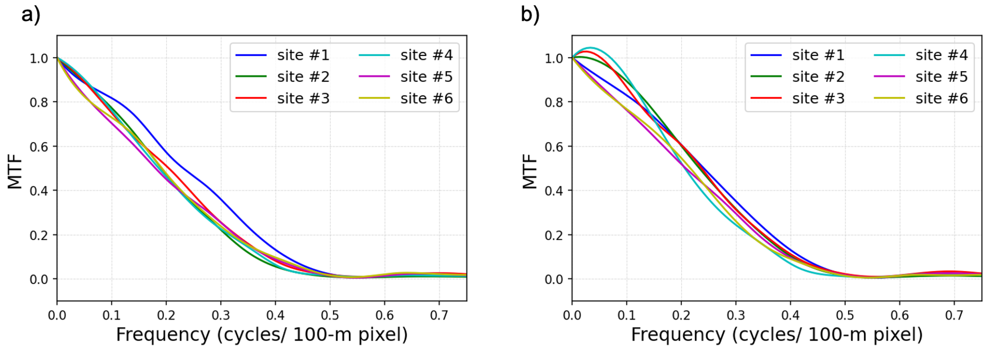
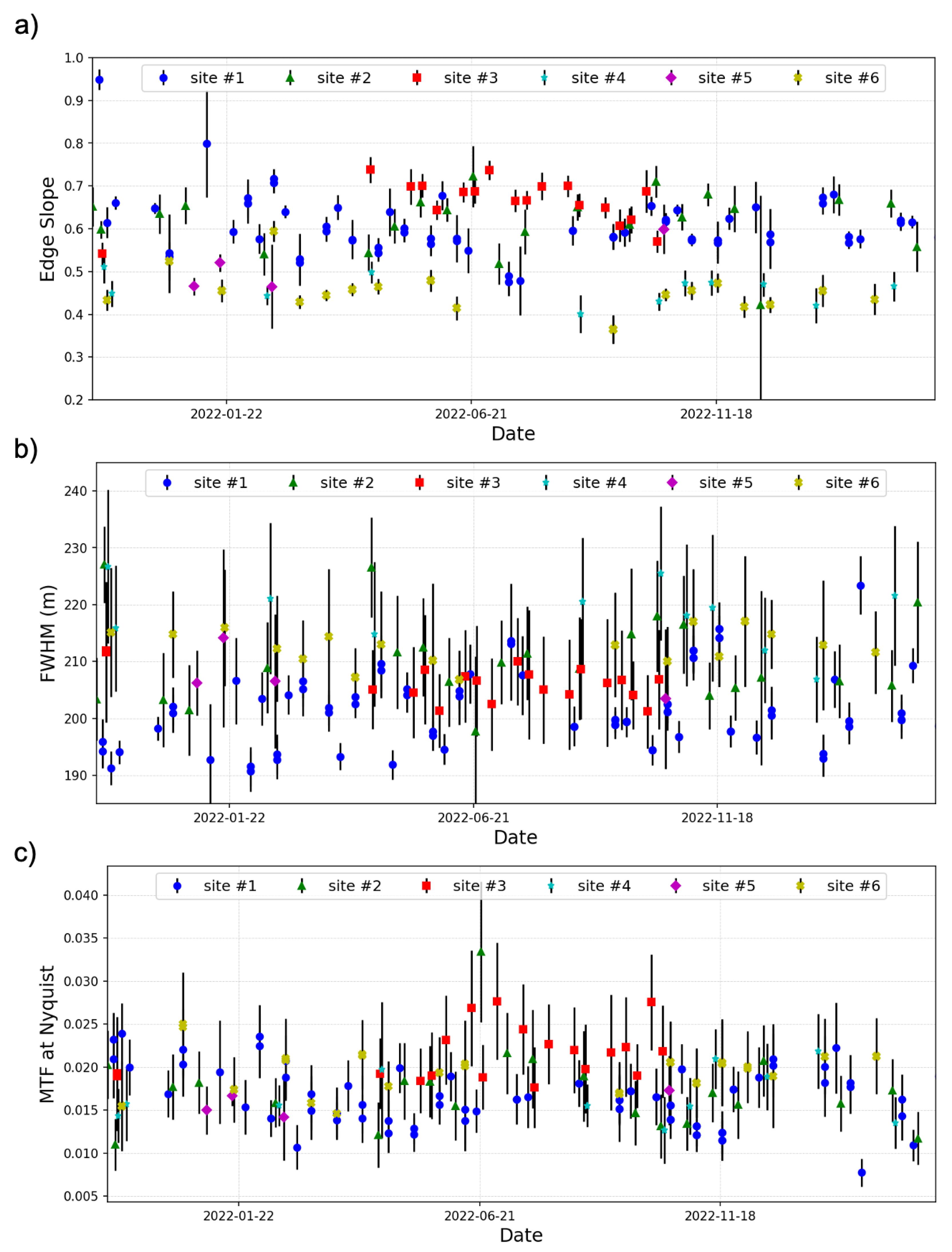
3.2. Post-Launch Analysis

The ESF, LSF, and MTF generated for the edge target site #6 (Table 2) for both L9 and L8 is shown in Figure 12. The results are reported for only band 10 of the TIRS instruments, since similar results were observed for both bands. The edge was oriented in the along-track direction for this particular site. The telescope was at the nominal temperature set-point for both L9/L8. The addition of the linear term, as described in Section 2.3, produced fairly uniform data on each side of the edge (Figure 12b,f). Note that we have limited the data to show only ±20 pixels. The measured SNR for L9 and L8 for site #6 is 54 and 67, respectively. Previous studies have shown that an SNR value of 50 or greater produced accurate estimations of the PSF/MTF. Despite the high SNR values, we still noticed significant noise/variability in the produced LSF function (Figure 12c,g). As expected, the noise was more prominent on the warmer, non-uniform land side of the edge target. The FWHM of L9/L8 was 7.210 and 7.095 pixels, respectively, for the L1T product at the 30 m GSD. If we consider the 100 m native resolution of the TIRS instrument, the FWHM translates to 216 m (std. dev. = 12.88 m) and 210 m (std. dev. = 10.33 m) for L9/L8, respectively, while the value of the MTF at Nyquist for both L9/L8 at the native 100 m GSD is 0.016 and 0.014 cycles/100-m pixel, respectively. The measured edge slope, FWHM, and MTF at Nyquist for the edge target site #6 is very similar for both TIRS instrument on L9/L8 at the nominal telescope temperature. This was a good early indicator of the spatial performance of L9 on orbit, when compared against L8, during the commissioning phase. Similar results were obtained for edges oriented in the across-track direction, which is shown in Figure 13 for site #1. The telescope was also at the nominal temperature set-point for both L9/L8.
A summary of the data for all six test sites for band 10 during the focusing test is detailed in Table 4. The mean and standard deviation of the edge slope, the FWHM at the 100 m native resolution, and the MTF at Nyquist for a 100 m pixel are reported. The MTF plots for all the edge targets are also shown in Figure 14. Similarly, the edge slope, FWHM, and MTF at Nyquist were produced between L9 and L8 during the commissioning phase when the telescope temperature was varied by ±4 K. Changing the telescope temperature by +4 K (sites #4 and #5) had an insignificant impact on the spatial performance. The biggest difference in the PSF/MTF estimations between L9 and L8 were noticed for sites #2 and #3, where the telescope temperature was changed by −4 K. Site #2 produced the worst performance for L9 when compared to L8 with a measured FWHM difference of 20 m. Although the differences were still within the uncertainty of what can be expected from naturally occurring edge target sites, we concluded that there was insufficient evidence of a focus shift through launch, and the telescope temperature was, therefore, kept at its pre-determined nominal set-point. Note the the images for L9/L8 were not collected coincidentally, which introduced a level of uncertainty to the measurement. The spatial quality was also fairly consistent between all sites, during the commissioning phase, which can be seen in the MTF plots in Figure 14.
The spatial performance of L9 on orbit was also monitored over time for the six mentioned sites. Figure 15 shows the change in the edge slope, FWHM, and MTF at Nyquist for these sites from November 2021 to April 2023. The accuracy of the PSF/MTF estimation remained fairly consistent across the six sites and over time. The measured uncertainty for the FWHM remained less than 2% for all the sites, while the average standard deviation of the edge slope and MTF at Nyquist across all sites was 0.02 and 0.003 cycles/100 m pixel, respectively. The highest variability was observed for site #4, which had the largest mean FWHM value of 219 m over the time span. The PSF/MTF estimations from site #1 consistently produced the best results. The average edge slope, FWHM, and MTF at Nyquist for site #1 were 0.613, 201 m, and 0.017, respectively. As these targets are not ideal “knife-edge” targets, there were inherent uncertainties associated with accurately estimating the PSF/MTF using on-orbit data. Despite the site selection criteria described in Section 2.3, the shorelines were still going through changes over time and introduced a level of error to the measurements. In the results from the post-launch analysis, we expected to see additional blurring in the along-track direction due to the orbital motion of the sensor. However, we did not notice significant differences in the PSF/MTF estimations between the along-track (sites #2, #4, #5, and #6) and across-track (sites #1 and #3) directions. Figure 15 only shows measurements for SNR > 50. This guideline seemed to hold for accurate measurements of the edge; however, a greater SNR did not always yield better results. The SNR measurement (Equation (3)) takes into account the uniformity of the water/land and the thermal contrast between them. It does not take into account the sharpness of the edge. A better measure of the SNR, in the future, should consider these factors.

4. Conclusions and Summary

The TIRS-2 instrument continues the thermal band observations of the Earth as part of the L9 mission. The spatial response of the TIRS-2 instrument is a crucial characteristic for assessing image performance and provides users with a metric to articulate the optical sharpness of the acquired data. This paper documents the effort to characterize the spatial performance of the TIRS-2 instrument in pre-launch testing under the TVAC condition. Additionally, we evaluated the spatial response on orbit using naturally occurring Earth edge targets to confirm that the optical system remained stable, thereby ensuring that image quality was not compromised due to any shifts during launch. The common metrics for spatial performance of the edge slope, edge extent, and MTF were carefully measured both pre-launch and on orbit.
The TIRS-2 spatial requirement sets the edge slope to be greater than 0.47 and the edge extent to be less than 240 m for a 100 m pixel. During ground testing, a controlled knife-edge target was swept across the FOV of the sensor to produce an over-sampled edge response function from which the ESF and MTF were derived. The measured edge slope, edge extent, and MTF for bands 10 and 11 of TIRS-2 in both the along- and across-track direction is summarized in Table 3. The measured spatial response metrics did meet the TIRS-2 spatial requirements at pre-launch. Table 3 also summarizes the edge slope and extent for the TIRS-1 sensor on L8. The results revealed similar optical performance between the two TIRS sensors on L8/L9, with the edge extent in the 200 to 230 m range. The MTF of TIRS-2 was also measured during the TVAC, which is shown in Figure 5c, while the MTF value at Nyquist for TIRS-2 is summarized in Table 3. The MTF value at Nyquist was approximately ∼0.54 cycles/pixel for the TIRS-2 instrument when measured in TVAC. The MTF analysis is not part of the spatial requirement for TIRS-2, but is included for comparison with the derived MTF on orbit.
To ensure no optical changes occurred during launch, spatial measurements were also repeated on orbit during instrument commissioning by utilizing high-contrast water/land boundaries as a substitute for knife-edge targets. The development of a man-made target for TIRS-2 on-orbit ESF estimation is impractical due to the large IFOV of the Landsat thermal sensor; thus, naturally occurring thermal edge targets were identified. The six chosen sites and the criteria to select them are detailed in Section 2.3. The spatial response of these sites was measured during a focusing test, during which the telescope temperature of TIRS-2 was changed by ±4 K from the nominal value of 190 K. The measured edge slope, edge extent, and MTF for bands 10 and 11 of TIRS-2 (L9) and TIRS-1 (L8) for these six naturally occurring sites is summarized in Table 4. Changing the telescope temperature of TIRS-2 had a minimal impact on the spatial performance when compared to TIRS-1. The differences were within the uncertainty of what can be expected from naturally occurring edge target sites. The consistency of the spatial performance for both TIRS-2 and TIRS-1 was also evident in the measured MTF across all six sites, as depicted in Figure 14. As a result, we concluded that the telescope temperature should be kept at its pre-determined nominal set-point. Given the minimal impact of telescope temperature changes on spatial performance, future designs can consider incorporating adaptive or more resilient optical systems that can further minimize the impact of environmental variables. The spatial performance of TIRS-2 post-launch was also monitored for the six mentioned sites from November 2021 to April 2023, which is shown in Figure 15. The accuracy of the PSF/MTF estimations remained consistent over time for all six sites. This served as a positive indication that TIRS-2 has been performing as intended in its nominal operational setting, with no discernible impact on the spatial quality over an approximately two-year period since launch.
It is difficult to directly compare the PSF/MTF measurements determined pre- and post-launch. The pre-launch analysis was performed on the raw imagery data from the TIRS-2 sensor, while the post-launch analysis was performed on the standard product produced by the Landsat Ground Processing System. Similar measurements of the edge extent were observed pre- and post-launch. The edge extent pre-launch estimate ranged between 200 and 230 m, while the post-launch estimate ranged between 195 and 226 m. The discrepancy in the pre- and post-launch estimates can be most seen in the measured MTF. The MTF value at Nyquist was approximately ∼0.54 cycles/pixel and ∼0.002 cycles/100 m pixel for the TIRS-2 instrument when measured in TVAC and post-launch, respectively. Note that the TIRS-2 detectors produce a GSD of approximately 100 m for each spectral band, which is spatially resampled from image sensor coordinates to a UTM grid and upsampled to 30 mpixels to be consistent with the OLI-2 sensor. The resampling process applied to the TIRS data on orbit is most likely the cause for the disparities between the measured MTF in TVAC and post-launch. Utilizing coastlines as naturally occurring slanted edge targets for the PSF/MTF assessment also introduced a degree of uncertainty into the post-launch measurements.
These variations between pre- and post-launch predominantly stemmed from uncertainties inherent in the estimation process, and there is likely no degradation of the TIRS-2 focus occurring over the timeframe between launch and operational imaging. This was also confirmed by the consistency in the spatial performance of TIRS-2 on L9 when compared against TIRS-1 on L8 over the same on-orbit target sites. Overall, users can expect very similar spatial performance between the two TIRS instruments on Landsat 8 and 9 with PSF widths of approximately 200 m. Additionally, the methodology outlined in this manuscript can be used as a template to track technological advancements and improvements in the spatial response and image quality of future Earth-observing missions.

Author Contributions

Conceptualization, R.E. and B.N.W.; Methodology, R.E. and B.N.W.; Validation, R.E. and B.N.W.; Formal analysis, R.E., B.N.W., E.P. and S.E.K.; Investigation, R.E. and B.N.W.; Data curation, B.N.W. and M.M.; Writing—original draft, R.E., B.N.W. and M.M.; Writing—review & editing, R.E., B.N.W., M.M. and A.G.; Supervision, A.G. and K.J.T.; Project administration, A.G. and K.J.T. All authors have read and agreed to the published version of the manuscript.

Funding

This material is based upon work supported by the National Aeronautics and Space Administration (NASA) under the Cooperative Agreement 80NSSC19K1694.

Data Availability Statement

Data available on request.

Conflicts of Interest

The authors declare no conflict of interest.

References

  1. Masek, J.G.; Wulder, M.A.; Markham, B.; McCorkel, J.; Crawford, C.J.; Storey, J.; Jenstrom, D.T. Landsat 9: Empowering open science and applications through continuity. Remote Sens. Environ. 2020, 248, 111968. [Google Scholar] [CrossRef]
  2. Choate, M.J.; Rengarajan, R.; Hasan, M.N.; Denevan, A.; Ruslander, K. Operational Aspects of Landsat 8 and 9 Geometry. Remote Sens. 2023, 16, 133. [Google Scholar] [CrossRef]
  3. Eon, R.; Gerace, A.; Falcon, L.; Poole, E.; Kleynhans, T.; Raqueño, N.; Bauch, T. Validation of Landsat-9 and Landsat-8 Surface Temperature and Reflectance during the Underfly Event. Remote Sens. 2023, 15, 3370. [Google Scholar] [CrossRef]
  4. Pagnutti, M.; Blonski, S.; Cramer, M.; Helder, D.; Holekamp, K.; Honkavaara, E.; Ryan, R. Targets, methods, and sites for assessing the in-flight spatial resolution of electro-optical data products. Can. J. Remote Sens. 2010, 36, 583–601. [Google Scholar] [CrossRef]
  5. Wenny, B.N.; Helder, D.; Hong, J.; Leigh, L.; Thome, K.J.; Reuter, D. Pre-and post-launch spatial quality of the Landsat 8 Thermal Infrared Sensor. Remote Sens. 2015, 7, 1962–1980. [Google Scholar] [CrossRef]
  6. Storey, J.C. Landsat 7 on-orbit modulation transfer function estimation. In Sensors, Systems, and Next-Generation Satellites V; SPIE: Bellingham, WA, USA, 2001; Volume 4540, pp. 50–61. [Google Scholar]
  7. Hair, J.; Reuter, D.; Tonn, S.; McCorkel, J.; Simon, A.; Djam, M.; Alexander, D.; Ballou, K.; Barclay, R.; Coulter, P.; et al. Landsat 9 Thermal Infrared Sensor 2 Architecture and Design. In Proceedings of the IEEE International Geoscience and Remote Sensing Symposium (IGARSS), Valencia, Spain, 22–27 July 2018; pp. 8841–8844. [Google Scholar] [CrossRef]
  8. Montanaro, M.; McCorkel, J.; Tveekrem, J.; Stauder, J.; Mentzell, E.; Lunsford, A.; Hair, J.; Reuter, D. Landsat Thermal Infrared Sensor 2 Stray Light Mitigation and Assessment. IEEE Trans. Geosci. Remote Sens. 2022, 60, 1–8. [Google Scholar] [CrossRef]
  9. Gerace, A.; Kleynhans, T.; Eon, R.; Montanaro, M. Towards an operational, split window-derived surface temperature product for the thermal infrared sensors onboard Landsat 8 and 9. Remote Sens. 2020, 12, 224. [Google Scholar] [CrossRef]
  10. Cawse-Nicholson, K.; Townsend, P.A.; Schimel, D.; Assiri, A.M.; Blake, P.L.; Buongiorno, M.F.; Campbell, P.; Carmon, N.; Casey, K.A.; Correa-Pabón, R.E.; et al. NASA’s surface biology and geology designated observable: A perspective on surface imaging algorithms. Remote Sens. Environ. 2021, 257, 112349. [Google Scholar] [CrossRef]
  11. Melton, F.S.; Huntington, J.; Grimm, R.; Herring, J.; Hall, M.; Rollison, D.; Erickson, T.; Allen, R.; Anderson, M.; Fisher, J.B.; et al. OpenET: Filling a critical data gap in water management for the western United States. JAWRA J. Am. Water Resour. Assoc. 2022, 58, 971–994. [Google Scholar] [CrossRef]
  12. Viallefont-Robinet, F.; Helder, D.; Fraisse, R.; Newbury, A.; van den Bergh, F.; Lee, D.; Saunier, S. Comparison of MTF measurements using edge method: Towards reference data set. Opt. Express 2018, 26, 33625–33648. [Google Scholar] [CrossRef] [PubMed]
  13. Choi, T.; Helder, D.L. Generic sensor modeling for modulation transfer function (MTF) estimation. In Proceedings of the Pecora, Sioux Falls, SD, USA, 23–27 October 2005; Volume 16, pp. 23–27. [Google Scholar]
  14. Forshaw, M.; Haskell, A.; Miller, P.; Stanley, D.; Townshend, J. Spatial resolution of remotely sensed imagery A review paper. Int. J. Remote Sens. 1983, 4, 497–520. [Google Scholar] [CrossRef]
  15. ISO 12233: 2000; Photography–Electronic Still Picture Cameras–Resolution Measurements. International Organization for Standardization: Geneva, Switzerland, 2000.
  16. Burns, P.D. Slanted-edge MTF for digital camera and scanner analysis. In Proceedings of the IS and Ts PICS Conference, Portland, OR, USA, 26–29 March 2000; pp. 135–138. [Google Scholar]
  17. Kohm, K. Modulation transfer function measurement method and results for the Orbview-3 high resolution imaging satellite. In Proceedings of the ISPRS, Istanbul, Turkey, 12–23 July 2004; Volume 35, pp. 12–23. [Google Scholar]
  18. Helder, D.; Choi, T.; Rangaswamy, M. In-flight characterization of spatial quality using point spread functions. In Post-Launch Calibration of Satellite Sensors; CRC Press: Boca Raton, FL, USA, 2004; pp. 159–198. [Google Scholar]
  19. McCorkel, J.; Montanaro, M.; Efremova, B.; Pearlman, A.; Wenny, B.; Lunsford, A.; Simon, A.; Hair, J.; Reuter, D. Landsat 9 thermal infrared sensor 2 characterization plan overview. In Proceedings of the IGARSS 2018—2018 IEEE International Geoscience and Remote Sensing Symposium, Valencia, Spain, 22–27 July 2018; pp. 8845–8848. [Google Scholar]
  20. Montanaro, M.; Levy, R.; Markham, B. On-orbit radiometric performance of the Landsat 8 Thermal Infrared Sensor. Remote Sens. 2014, 6, 11753–11769. [Google Scholar] [CrossRef]
  21. Montanaro, M.; Gerace, A.; Lunsford, A.; Reuter, D. Stray light artifacts in imagery from the Landsat 8 Thermal Infrared Sensor. Remote Sens. 2014, 6, 10435–10456. [Google Scholar] [CrossRef]
  22. Montanaro, M.; Gerace, A.; Rohrbach, S. Toward an operational stray light correction for the Landsat 8 Thermal Infrared Sensor. Appl. Opt. 2015, 54, 3963–3978. [Google Scholar] [CrossRef]
  23. Choi, T.; Xiong, X.; Wang, Z. On-orbit lunar modulation transfer function measurements for the moderate resolution imaging spectroradiometer. IEEE Trans. Geosci. Remote Sens. 2013, 52, 270–277. [Google Scholar] [CrossRef]
  24. Press, W.H.; Teukolsky, S.A. Savitzky-Golay smoothing filters. Comput. Phys. 1990, 4, 669–672. [Google Scholar] [CrossRef]
  25. Tanaka, T.; Sato, Y.; Kusakawa, Y.; Shimizu, K.; Tanaka, T.; Kim, S.K.; Komatsu, M.; Yoo, I.; Caesy, L.; Nakasuka, S. The operation results of earth image acquisitionusing extensible flexible optical telescope of “PRISM”. In Proceedings of the 27th International Symposium on Space Technology and Science (ISTS), Tsukuba, Japan, 5–12 July 2009. [Google Scholar]
  26. Shrivakshan, G.; Chandrasekar, C. A comparison of various edge detection techniques used in image processing. Int. J. Comput. Sci. Issues (IJCSI) 2012, 9, 269. [Google Scholar]
Figure 1. Graphical illustration to construct the oversampled ESF from a slanted-edge target.
Remotesensing 16 01065 g001
Figure 2. A schematic layout of the CGSE and TIRS-2.
Remotesensing 16 01065 g002
Figure 3. The CGSE mounted in the TVAC chamber during the lab geometric characterization and calibration of the TIRS-2 sensor at the NASA GSFC facilities.
Remotesensing 16 01065 g003
Figure 4. (a) TIRS-2 raw image of circular target used for spatial analysis, (b) normalized cross-sections of all rows through the target, (c) all peak response cross-sections for the 80 images acquired during the sub-pixel movement.
Remotesensing 16 01065 g004
Figure 5. (a) Cross-sections from Figure 4c shifted to a common reference frame, (b) the left edge of the response, and (c) the calculated MTF of the system.
Remotesensing 16 01065 g005
Figure 6. Workflow describing the estimation of the (b,c) ESF, (d) LSF and (e) MTF using the modified Fermi function applied to (a) simulated sinc function for on-orbit spatial assessment of the TIRS-2 sensor.
Remotesensing 16 01065 g006
Figure 7. The location of the 6 naturally occurring target edge sites to perform the spatial assessment of the TIRS-2 sensor on orbit.
Remotesensing 16 01065 g007
Figure 8. The measured edge slope for band 10 across the FOV of the sensor during TVAC1 and TVAC2 for both the across- (upper) and along- (lower) track direction. The edge slope requirement of 0.47 for TIRS-2 is shown by the dashed red line.
Remotesensing 16 01065 g008
Figure 9. The measured edge slope for band 11 across the FOV of the sensor during TVAC1 and TVAC2 for both the across- (upper) and along- (lower) track direction. The edge slope requirement of 0.47 for TIRS-2 is shown by the dashed red line.
Remotesensing 16 01065 g009
Figure 10. The measured edge extent for band 10 across the FOV of the sensor during TVAC1 and TVAC2 for both the across- (upper) and along- (lower) track direction. The edge extent requirement of 240-m for TIRS-2 is shown by the dashed red line.
Remotesensing 16 01065 g010
Figure 11. The measured edge extent for band 11 across the FOV of the sensor during TVAC1 and TVAC2 for both the across- (upper) and along- (lower) track direction. The edge extent requirement of 240-m for TIRS-2 is shown by the dashed red line.
Remotesensing 16 01065 g011
Figure 12. The ESF, LSF, and MTF measured for the edge site location #6 for the TIRS sensor on board L9 (ad) and L8 (eh).
Remotesensing 16 01065 g012
Figure 13. The ESF, LSF, and MTF measured for the edge site location #1 for the TIRS sensor on board L9 (ad) and L8 (eh).
Remotesensing 16 01065 g013
Figure 14. The measured MTF for the (a) L9 and (b) L8 TIRS sensor at the native 100 m resolution for all 6 target sites.
Remotesensing 16 01065 g014
Figure 15. The measured (a) edge slope, (b) FWHM, and (c) MTF at Nyquist for the TIRS-2 sensor on board L9 for the 6 selected sites from November 2021 to April 2023. The figure demonstrates the consistent performance of TIRS-2 spatial quality across various sites and over time.
Remotesensing 16 01065 g015
Table 1. Focusing test schedule for the TIRS-2 sensor during commissioning.
Focusing Test ScheduleTelescope Temperature (K)Edge Site Location
Before 5 November 2021 14:30 UTC190 (nominal focus)#1
Between 5 November 2021 17:30 and 7 November 2021 15:30 UTC186 (−4 K)#2 and #3
Between 7 November 2021 21:30 and 9 November 2021 14:50 UTC194 (+4 K)#4 and #5
After 9 November 2021 19:30 UTC190 (nominal focus)#6
Table 2. Detailed information on the 6 naturally occurring target edge sites during the focusing test.
Edge Site LocationPath/RowLat., Lon.DateDirectionTelescope Temperature (K)
#1157/04225.4489, 59.295 November 2021Across-Track190
#2179/077−27.736, 14.7526 November 2021Along-Track186
#3186/03830.997, 17.5607 November 2021Across-Track186
#4161/0548.700, 50.3828 November 2021Along-Track194
#5183/071−15.865, 11.7359 November 2021Along-Track194
#6157/04520.877, 58.74910 November 2021Along-Track190
Table 3. Summary of the edge slope, edge extent, and MTF at Nyquist pre-launch results for 10.8- μ m (band 10) and 12.0- μ m (band 11) in the across- and along-track directions for both TIRS-1 and TIRS-2. The MTF is reported for only TIRS-2.
Edge SlopeEdge Extent (m)MTF Value at Nyquist
TIRS-2TIRS-1TIRS-2TIRS-1TIRS-2
10.8 XT0.58 (0.01)0.59 (0.02)222.8 (7.4)202.8 (9.1)0.542 (0.01)
10.8 AT0.55 (0.01)0.53 (0.03)230.8 (4.4)234.0 (17.1)0.516 (0.04)
12.0 XT0.59 (0.01)0.61 (0.01)211.7 (4.9)197.6 (6.9)0.548 (0.01)
12.0 AT0.60 (0.01)0.63 (0.02)205.6 (5.2)184.3 (10.9)0.556 (0.02)
Table 4. Summary of the edge slope, FWHM, and MTF at Nyquist for all test sites for band 10 in L9/L8 during the focusing test.
Edge Site LocationSNREdge SlopeFWHM (m)MTF Value at Nyquist
L9 L8 L9 L8 L9 L8 L9 L8
#1931050.647 [0.027]0.654 [0.018]195 [3.54]196 [3.60]0.020 [0.004]0.019 [0.003]
#2731140.586 [0.022]0.636 [0.036]226 [7.21]206 [6.14]0.010 [0.004]0.015 [0.004]
#360990.507 [0.031]0.697 [0.035]215 [8.06]206 [4.55]0.018 [0.006]0.022 [0.005]
#490630.492 [0.034]0.531 [0.087]226 [13.75]228 [15.09]0.016 [0.004]0.013 [0.002]
#554680.377 [0.036]0.471 [0.010]213 [4.45]206 [6.58]0.015 [0.004]0.018 [0.004]
#654670.425 [0.023]0.480 [0.021]216 [12.88]212 [10.33]0.017 [0.005]0.014 [0.004]
Disclaimer/Publisher’s Note: The statements, opinions and data contained in all publications are solely those of the individual author(s) and contributor(s) and not of MDPI and/or the editor(s). MDPI and/or the editor(s) disclaim responsibility for any injury to people or property resulting from any ideas, methods, instructions or products referred to in the content.

