Article

High-Resolution Remote Sensing of the Gradient Richardson Number in a Megacity Boundary Layer

1
School of Geoscience and Technology, Zhengzhou University, Zhengzhou 450001, China
2
State Key Laboratory of Atmospheric Boundary Layer Physics and Atmospheric Chemistry, Institute of Atmospheric Physics, Chinese Academy of Sciences, Beijing 100029, China
3
Shanghai Investigation, Design, and Research Institute, Shanghai 200093, China
4
College of Earth and Planetary Sciences, University of Chinese Academy of Sciences, Beijing 100049, China
*
Author to whom correspondence should be addressed.
Remote Sens. 2024, 16(6), 1075; https://doi.org/10.3390/rs16061075
Submission received: 5 January 2024 / Revised: 9 March 2024 / Accepted: 10 March 2024 / Published: 19 March 2024

Abstract

:
The Gradient Richardson Number (Ri) is an important parameter for appraising the stability and turbulence exchange at the atmospheric boundary layer (ABL). However, high-resolution measurements of Ri profiles are rarely reported, especially in megacities. In this study, a Doppler wind lidar and a microwave radiometer were simultaneously utilized to measure the 2 km Ri vertical profile in downtown Beijing. These measurements were verified to have high accuracy compared with observations from a 325 m meteorological tower, with root-mean-square errors (RMSEs) of less than 1.66 K, 7.9%, and 1.45 m/s for the temperature, relative humidity, and wind speed (WS) for all altitudes and corresponding Pearson correlation coefficients (R) of 0.97, 0.93, and 0.81. The inter-comparisons of different spatial (25 m, 50 m, 100 m) and temporal resolutions (1 min, 30 min, 1 h) form a 3 × 3 resolution matrix of Ri, in which the 1 h temporal resolution of Ri overestimates the intensity and active area of turbulence. The Ri value retrieved from the 100 m spatial resolution data overestimates these by half as it misidentifies the height of the stable area at the near surface. There are significant differences between the data with a 1 min temporal resolution and a 25 m spatial resolution (defined as the standard resolution of Ri), and the rest of the data in the resolution matrix (defined as data at other resolutions), with an RMSE > 1 and an R < 0.8. The difference between data at the standard resolution and data at other resolutions increases with elevations, which results from frequent weather processes or from water-vapor blocking at higher altitudes. The Ri profiles reveal that the atmospheric layer at altitudes from 100 m to 500 m in daytime is unstable, with Ri < 0, while it is neutral, with 0 < Ri < 0.25, at night-time from 200 m to 400 m. The atmosphere above the ABL in a megacity is rather stable, with Ri > 0.25, whereas below the ABL, it is neutral or unstable, which is due to drastic changes in the WS and temperature that are affected by the topography and surface friction.

Graphical Abstract

1. Introduction

The Gradient Richardson Number (Ri), named after Lewis Fry Richardson, is a dimensionless number that is defined as the ratio of thermal buoyancy to wind shear. It is an important parameter for determining the generation of turbulence and the hydrostatic stability of a fluid. Therefore, the concept of Ri is widely applied in the field of atmospheric science [1,2,3], such as in the estimation of the atmospheric boundary-layer height (ABLH), the modeling of mixed layers [4], and the quantification of the night-time boundary layer [5]. In general, it is well recognized that the atmosphere is unstable when Ri is smaller than a certain critical value of 0.25, and the stability tends to be enhanced with the increase in Ri [6].
The ABL, a key transitional zone between the Earth’s surface and the free atmosphere, is directly affected by surface features, solar radiation, and WS, which can be theoretically classified as stable, neutral, and unstable according to the state of atmospheric stratification based on distinct physical properties [7]. An important feature of the atmospheric motion within the ABL is the ubiquitous turbulence that plays a vital role in the vertical transport of heat, momentum, and water vapor [8,9,10]. Therefore, probing the structural characteristics of the ABL is of great importance in improving the accuracy of prediction models of weather, climate, and atmospheric environmental quality, as well as for the development and extinction of clouds, convection, and atmospheric pollution.
Various approaches have been developed in the past decades for the investigation of the ABL. For example, layered observations from the 325 m tower were used to evaluate the influence of the urban boundary-layer structure on the accumulation of atmospheric pollutants [11], although these were only available at the near surface. Radio sounding has advantages in terms of the vertical resolution and range, making it an effective means for deriving the boundary-layer height [12]. However, the boundary-layer heights estimated from radio soundings have limitations in their temporal resolution because of the regularly fixed-time operations and also a horizontally large drift. Vertical temperature profiles retrieved from passive techniques such as infrared and microwave space-borne remote sensing technologies have a spatial resolution of 1–2 km, which is too coarse to meet the requirement for analyzing structural profiles of the ABL. In recent years, with the rapid development of in situ remote sensing instruments such as the Doppler wind lidar [13,14,15] and the microwave radiometer [16], it is achievable for us to accurately measure the meteorological data at finer spatiotemporal resolutions.
Beijing, the capital of China, is a typical megacity with a non-uniform complex underlying surface, and its ABL characteristics as a representative of megacities have become a hot issue in ABL research fields all over the world [17]. For the purpose of better exploring the characteristics of the ABL in downtown Beijing, Ri values retrieved from different resolution datasets have been analyzed, which will provide scientific references for the selection and application of different-resolution datasets in evaluating atmospheric stability and also deepen our understanding regarding urban ABL structures.

2. Sites, Instruments, and Methods

2.1. Introduction to the IAP Integrated Observatory

Figure 1a shows the geographic location of the observatory and its surrounding environment, and Figure 1b shows the urban landscape of downtown Beijing. The observation site is the State Key Laboratory of Atmospheric Boundary Layer Physics and Atmospheric Chemistry, Institute of Atmospheric Physics, Chinese Academy of Sciences (IAP, CAS: 39°58′N, 116°22′E, 49 m), hereafter referred to as the IAP integrated observatory. Measurements were performed during 1–25 January 2019 using the 325 m meteorological tower, a microwave radiometer, a Doppler wind lidar, and a CL51 ceilometer (Figure 1c–f) in order to measure the wintertime thermodynamic ABL.

2.2. Instruments

2.2.1. IAP 325 m Tower

The 325 m meteorological tower has the advantages of high accuracy and the simultaneous observation of multiple layers. The 325 m meteorological tower has seventeen levels of operating platforms, of which fifteen platforms are commonly used, i.e., those at 8, 15, 32, 47, 63, 80, 102, 120, 140, 160, 180, 200, 240, 280, and 320 m. Each level is equipped with two anemometers (wind cups), one anemometer (wind vane), one thermometer, one hygrometer, and one data collector. The platform is 0.7 m in width, and the protective railing is around 1 m in height. The 325 m meteorological tower is capable of measuring the multi-meteorological variables of temperature, relative humidity, horizontal WS, and horizontal wind direction (WD). To date, the IAP 325 m meteorological tower has accumulated meteorological data for more than 40 years, which can be regarded as a reference basis for other observational approaches.

2.2.2. Microwave Radiometer

The microwave radiometer (HATPRO-G5, RPG, Meckenheim, Germany) is a passive microwave remote sensing device that can continuously acquire atmospheric thermal parameters such as temperature and humidity in the vertical range of 0–10 km in real time [18]. The microwave radiometer has two receivers, including seven frequency channels for water-vapor absorption lines (K-band 22.24–31.40 GHz) and seven frequency channels for oxygen absorption lines (V-band 51.26–58.00 GHz). A large amount of atmospheric radiation at frequencies of 22.24–31.40 GHz is actively radiated by water-vapor molecules, while atmospheric radiation at frequencies of 51.26–58.00 GHz is radiated by remotely sensed oxygen molecules [19]. The microwave radiometer is available in two modes: the zenith mode and the boundary-layer multi-angle scanning mode. In the zenith observation mode, the radiometer takes measurements only in the vertical channels. In the boundary-layer mode, all channels are sampled, and more information can be obtained. The two modes work together to achieve spatial resolution (60–300 m spatial resolution up to 10,000 m) and the boundary layer (25–40 m spatial resolution), with up to ninety-three layers in the vertical direction and a time resolution of 1 s. For more details, see http://www.radiometer-physics.de (last accessed on 3 November 2023).

2.2.3. Doppler Wind Lidar

The Doppler wind lidar (Windcube100s, Leosphere, Paris, France) is an active remote sensing device based on light detection and ranging techniques. The instrument has three observation modes: 1. The vertical DBS (Doppler beam swinging) scanning mode, known as the vertical profile mode; 2. The horizontal PPI (plan position indicator) scanning mode, known as the constant zenith-angle mode; 3. The tangential RHI (range height indicator) scanning mode, known as the constant azimuth mode. The detectable range of the instrument is from 50 m to about 3 km, of which the bottom limit of 50 m is the detection blind zone. The vertical resolutions are 20 m from 50 m to 300 m and 25 m for 300–3000 m. The time resolution of the WS is 5 s, with an integration time from 0.5 s to 10 s (standard integration time: 1 s), and the accuracy of WS is 0.5 m/s. The observation range of the radial WS and WD is −30 m/s to 30 m/s and 0 to 360°, respectively. More information about the instrument can be found at www.leosphere.com (last accessed on 3 November 2023).

2.2.4. CL51 Ceilometer

In this study, a CL51 ceilometer was used to obtain the height of the boundary layer. The ceilometer lidar (CL51, Vaisala, Vantaa, Finland) is an active remote sensing device. It is capable of emitting laser pulses and then receiving back the scattered signals caused by haze, fog, precipitation, and clouds. Based on the time interval between the signal transmission and reception, the height of the cloud bottom and the height of the boundary layer can be calculated. The CL51 ceilometer has a spatial resolution of 10 m and a temporal resolution of 15–16 s. For more information, please refer to www.vaisala.com (last accessed on 3 November 2023).

2.3. Methodology

2.3.1. ABL Thermal Parameters

Atmospheric temperature and humidity data obtained by microwave radiometers enable the calculation of atmospheric thermal parameters. The formulas are as follows:
P 2 = P 1 exp [ 1 R Z 1 Z 2 g T d z ]
θ = T × ( p 0 P ) R c p
e s = 6.1078 exp [ 17.2693882 T 273.16 T 35.86 ]
e = R H 100 × e s
q = 0.622 e p 0.378 e
θ v = θ ( 1 + 0.608 q )
where P, Z, θ, and T denote the actual pressure, altitude, potential temperature, and the temperature, respectively. P0 is the reference pressure of 1000 hPa, R represents the gas constant, and cp is the constant-pressure specific heat capacity of the air. In addition, es, e, q, and θv are the saturation vapor pressure, actual water-vapor pressure, specific humidity, and the virtual potential temperature, respectively.

2.3.2. Temperature Inversion

The formula for calculating the temperature lapse rate is as follows:
T e m p . I n v e r s i o n   ( i ) = 100 ( T i + 1 T i ) / ( Z i + 1 Z i )
where Ti denotes the atmospheric temperature at the i-th altitude (Zi). Temp.Inversion is the temperature lapse rate (unit: K/100 m). A positive temperature lapse rate (TI) demonstrates a stable atmosphere, while negative values usually indicate unstable stratification. When the TI is close to or equal to 0, it represents a neutral environment [20].

2.3.3. Gradient Richardson Numbers

The Ri equation was calculated using thermal parameters and wind field data, as follows:
R i = g θ v ( θ v / z ) ( u / z ) 2 + ( v / z ) 2
where θv denotes the virtual temperature, g is the gravitational acceleration, and z is the altitude. In practical calculations, the gradient of Equation (8) is approximated by finite differences as ∆θv/∆z, ∆u/∆z, and ∆v/∆z, where the increments of θ, u, and v over the vertical distance ∆z are taken from either actual observations or numerically simulated vertical profiles [21]. The numerator reflects the buoyancy disruption through the entire boundary layer, and the denominator is the estimation of the overall shear generation. In an aerodynamically stable environment, turbulence is opposite to the recovery force of gravity in the fluid motion, so buoyancy tends to inhibit turbulence, and wind shear is tilted toward mechanically generated turbulence.

3. Results

3.1. Comparative Validations of Multi-Source Data

3.1.1. Wind-Field Assessment

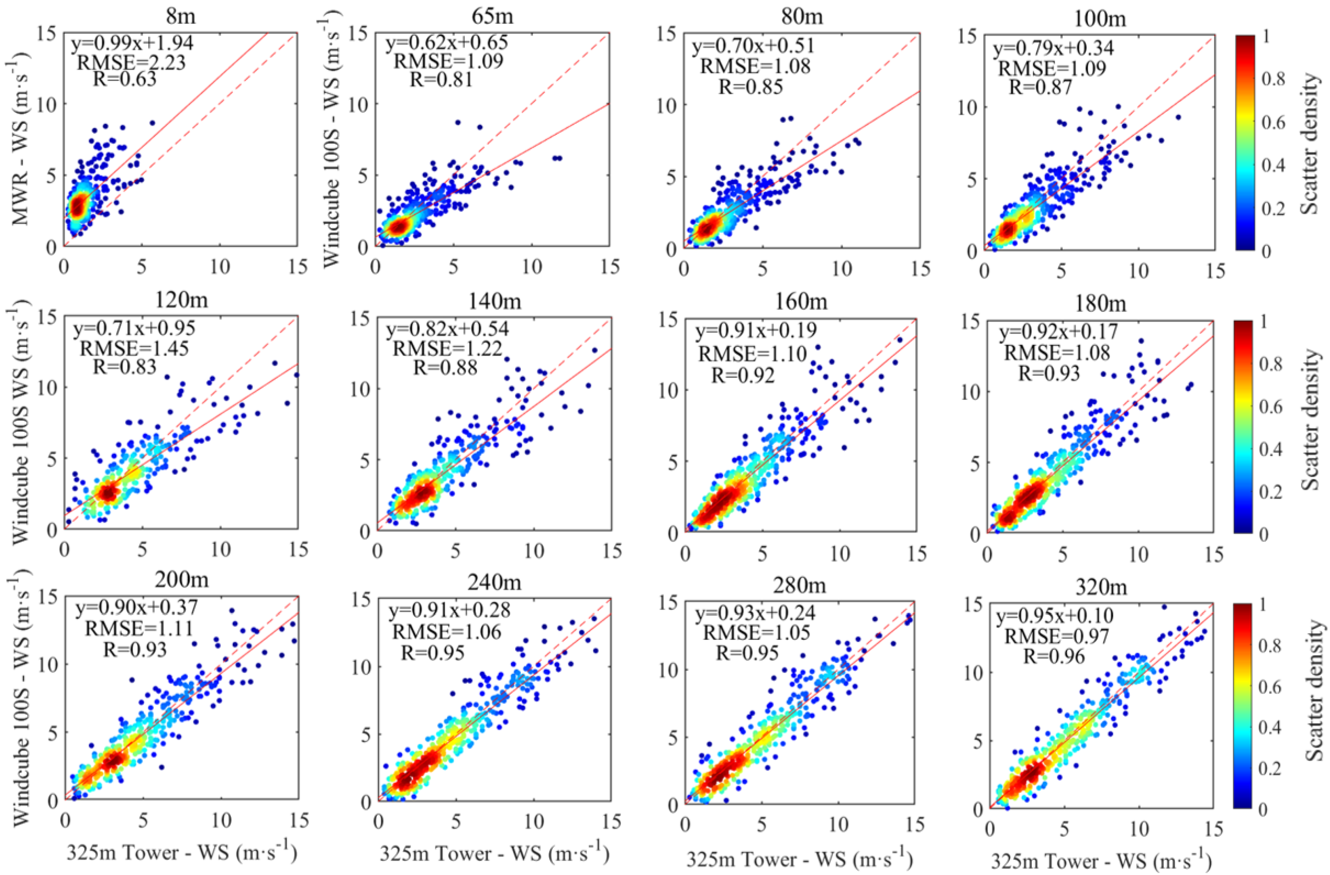
The horizontal WS measured by the Doppler wind lidar is similar to that measured by the 325 m tower at all vertical heights. As depicted in Figure 2, the WS observed by the Doppler wind lidar is slightly larger at low WS conditions, whereas it is underestimated compared with the tower observations in high WS scenarios.
The Pearson correlation coefficient (R) demonstrates an increasing trend with height, which indicates that the lidar observations are credible at higher altitudes. The R is around 0.9 at all heights except for that of 8 m. The Doppler wind lidar cannot measure the wind field below 50 m; therefore, we adopted the meteorological sensor mounted on the microwave radiometer for measuring the near-surface WS of 8 m. At this level, the surrounding buildings block the natural wind, leading to the smaller horizontal WS measured by the tower. Apart from the 8 m level, the horizontal WS measured by the Doppler wind lidar at an altitude of 120 m had the largest RMSE of 1.45 m/s compared with the tower observations. In summary, the detection bias of the Doppler lidar lies within an acceptable range, which proves that the Doppler wind lidar has a high degree of reliability.
Figure 3 shows the comparisons of the horizontal WS and WD detected by the Doppler wind lidar and the 325 m tower at various heights. The two similar curves are the averaged results of the Doppler wind lidar and the 325 m tower, respectively, which were obtained by dividing the WD into sixteen directions and averaging the WS into each WD bin at each height. Except for the blocked 8 m level, it is observed that the horizontal WS and WD detected by the Doppler wind lidar are in good agreement with those observed by the 325 m tower. Therefore, wind-field measured by the Doppler wind lidar has proven to be highly credible.

3.1.2. Temperature and Relative Humidity Assessment

According to Figure 4, the temperatures measured by the microwave radiometer at all heights are remarkably close to those measured by the 325 m tower, in which the Pearson correlation coefficient can be up to more than 0.97. In general, the temperature shows a decreasing trend with an increase in height, and the temperature measured by the microwave radiometer shows a cold deviation in comparison with the routine observation by the 325 m tower. The RMSE varies from 0.55 K at 8 m to 1.66 K at 320 m, with the median 0.94 K occurring at 140 m, so we can conclude that the difference between the two measuring approaches can be neglected and that the microwave radiometer also has a high degree of accuracy.
In Figure 5, the relative humidity (RH) measured by the microwave radiometer is likewise approximate to that measured by the 325 m tower, with the Pearson correlation coefficients ranging from 0.93 to 0.96. Generally, the RH tends to decrease with increasing elevations. The RMSE of the RH is 5.64% at 140 m, 7.9% at 80 m, and the median of 6.69% appears at 8 m. Moreover, the RH measured by the microwave radiometer exhibits a wet bias with respect to the 325 m tower observation below 120 m, and a dry bias in the range of 140–320 m. As the height increases, the deviation first decreases and then gradually increases, with the maximum deviation appearing at 320 m. In conclusion, the overall differences in the RH using these two technologies are rather small, and the microwave radiometer is capable of retrieving high-accuracy RH.

3.1.3. Comparison of Tower-Ri and Lidar-Ri

Figure 6 shows the inter-comparison of the calculated Lidar-Ri and Tower-Ri. It was found that the difference between the values of Lidar-Ri and Tower-Ri is large at 50 m, which then gradually decreases with increasing altitude. This phenomenon is mainly associated with the difference between the wind field observed by the Doppler wind lidar and the 325 m tower, as the temperature is highly consistent with each other. For humidity, this can only affect Ri indirectly through θv, and the effect is also minimal. Additionally, the positive and negative values of Lidar-Ri and Tower-Ri are approximately the same, and the trends of both Lidar-Ri and Tower-Ri are closer to each other with respect to elevation. Theoretical and experimental studies have shown that when Ri > 0, the atmosphere is always static and stable; when Ri < 0, turbulence starts to be active, and the atmosphere becomes unstable [22]. Therefore, below 300 m, Lidar-Ri can only qualitatively determine whether the atmosphere is stable or not, but it cannot accurately quantify the intensity of atmospheric stability.

3.2. Analysis of Gradient-Richardson-Number-Related Parameters

The variation in WS highly depends on the surface roughness and atmospheric stability [23]. The vertical variation in near-surface WS is mostly affected by surface roughness, and the larger the surface roughness is, the faster the WS decreases. Generally speaking, the variation in WS with height is smaller when the atmosphere is unstable because of the vertically turbulent transport of momentum [24]. Figure 7c shows the WD contour. The WD below 50 m is different from that above 50 m, which can be attributed to obstruction by the surrounding buildings. Changes in the WD at 500 m on 3, 6, and 11 January can be explained as being due to the influence of local circulations. Meanwhile, above 600 m, the WD remains unchanged.
Figure 8a shows the temperature observed by the microwave radiometer at a 25 m spatial resolution and 1 s temporal resolution. There is a roughly gradual increasing trend in the temperature from 1 to 25 January. The temperature reaches its maximum at noon on the 22nd and then suddenly drops on the 24th, which is probably due to the rainfall that occurred in the morning (Figure 8d). Figure 8c shows that the temperature inversions occur frequently at the near ground, as well as at the height of 1–2 km. Temperature inversion plays a vital role in determining cloud formation, precipitation, and visibility. The near-surface temperature inversion is possibly associated with the cooling properties of vegetation, water, and building shade inside the urban canopy. With regard to the temperature inversion present at 1–2 km, this always occurs when the WD is southwest (Figure 8b), which can be explained by the fact of the confrontation of warm and cold air masses. When warm air transported from the south over Beijing meets the cold air overhead of the city, the warm air is lifted up and forms a stratification of the cold lower layer and warm upper layer, which results in an advection temperature inversion at a certain height [25].
To further investigate the vertical structure of the temperature inversion, the variable “virtual potential temperature lapse rate” is introduced (∆θv = 2θ1) 100 ) using two neighboring layers on a vertical gradient, as shown in Figure 8e. The more continuous the zone of ∆θv > 0 is, the thicker the temperature-inverted layer is. The strength of the temperature inversion can be indicated by the magnitude of the value of ∆θv, with a larger ∆θv representing a stronger temperature inversion [26]. It was found that the temperature inversion occurs above 600 m and below 100 m, and that the intensity of inversion appears to be largest near the surface. The area of the temperature inversion region indicated by ∆θv is larger than that indicated by using TI.

3.3. Gradient-Richardson-Number Characterization

The Gradient Richardson Number (Ri) can be used to analyze the structure of the ABL and to estimate the height of the ABL [27,28]. The principle of identifying the height of the ABL is based on the difference in turbulent properties between the boundary layer and the free atmosphere, where the disappearance height of continuous turbulence can be identified as the height of the ABL [29]. Theoretical and experimental studies have proved that turbulence starts to appear when Ri < 0.25, and turbulence disappears when Ri > 0.25, so the height at Ri = 0.25 is chosen as the ABL height.
Generally, a critical value Ri = 0.25 is selected to determine the stability of the ABL. As shown in Figure 9, Ri < 0.25 represents the presence of turbulence;, otherwise there is no turbulence. Most of the Ri values are close to zero, demonstrating a frequent neutral atmosphere with minimal turbulent motions. In addition, turbulence persistently exists below a height of 500 m, and the strongest turbulence appears at around 300 m. Turbulence is very active during the midday to evening, mainly due to the high solar radiation during this period, which results in very strong atmospheric motions. Another phenomenon is that there are turbulent motions at night between 200 and 300 m, which is probably generated by local wind shear within the night-time boundary layer [30].
In Figure 9, the warm-tone fills correspond to stable layers with Ri > 0.25. It is interesting to find that there is a frequent temperature inversion existing at around 100 m. Above 500 m, it starts to be stable, and then the stability extends to a maximum of up to 1000 m. The buoyancy force dominates in this region, and the turbulence from wind shear is suppressed by laminar flow. However, a thin unsteady layer appears at around 1500 m. This is because the airflow above the maximum WS layer slows down faster; at the same time, the maximum WS layer oscillates with the decelerated airflow layer, leading to an increase in directional shear and a decrease in local Ri, thus increasing the probability of turbulence occurrence. These trends make the definition of the turbulent boundary layer more ambiguous, and the depth of the turbulent layer derived from Ri is significantly increased [31,32].
Ri is influenced by the temporal and spatial resolution. For the purpose of clarifying the differences in characterizing the ABL structure at different resolution datasets of Ri, nine resolution datasets of Ri are calculated and shown in Figure 9a–i. Among them, Figure 9c has a temporal resolution of 1 h and a spatial resolution of 100 m, with very few data dots that show the overall trend, while Figure 9g has a temporal resolution of 1 min and a spatial resolution of 25 m with plenty of data dots, allowing us to identify the precise values of Ri at each location. A lower temporal resolution overestimates the intensity of turbulence; for example, the blue unstable zone in Figure 9a becomes darker than that in Figure 9g. Moreover, it is difficult to capture the short-term change in Ri with a low time resolution, but it is easier to present the daily variations in Ri with a lower time resolution. For example, it can be clearly seen from Figure 9a that the daily change in Ri is more obvious from the 17th to the 21st. Similarly, lower spatial resolution would lead to larger altitude intervals, making it impossible to accurately estimate Ri at individual altitudes or even misidentifying the atmospheric stability. For example, at the same temporal resolution, Ri with a spatial resolution of 100 m is greater near the ground than that at 25 m, and Ri at a spatial resolution of 100 m overestimates the height of the turbulence onset by about 50% compared with that at 25 m.
In order to investigate the specific differences between different spatiotemporal resolution datasets of Ri, the 25 m/1 min-resolution Ri was adopted as the benchmark reference, and then we compared the Ri calculated from the remaining eight resolution datasets with the benchmark reference Ri to make the plots in Figure 10, where the horizontal and vertical axes represent the standard deviations, and the brown dashed lines represent the RMSE. In general, the RMSE of each resolution Ri versus the benchmark resolution Ri was greater than 1, and R was less than 0.8. It is thus evidenced that using a coarse-resolution Ri to characterize the atmosphere is not reliable.
The RMSEs of each resolution dataset of Ri to the benchmark resolution Ri is less than 2 below 600 m, with R in the range of 0.3 to 0.7, and the RMSE is greater than 2 from 800 m to 1500 m, with the correlation gradually weakening. This shows that the difference in Ri between the eight resolution datasets and the standard resolution dataset increasing with elevation is due to water vapor and cloud masking at high altitude. The differences in Ri among the three different spatial resolution datasets of inversions are smaller at altitudes from 600 m to 1000 m, because the atmosphere is neutral in this region and Ri is around 0. The 50 m/1 min resolution datasets of Ri have the smallest RMSEs with the benchmark resolution dataset at all altitudes, and the 1 h resolution datasets have the largest RMSEs with the benchmark resolution dataset of Ri, except for the 100 m/30 min resolution dataset of Ri at 100 m. This suggests that temporal resolution has a greater effect on Ri.
The standard deviations of Ri from different resolution datasets increase with elevation. For example, the standard deviation is less than 2 below 800 m and greater than 2 or even 2.5 above 800 m. The dramatic variations in Ri indicate rapid changes in atmospheric stability that are perturbed by frequent weather processes and large-scale circulations. Furthermore, the Ri values with low spatial but high temporal resolutions can show the changing trend of atmospheric stability, but it cannot accurately characterize the intensity of atmospheric stability. For example, at 600 m, the 100 m/1 min resolution has a better correlation of 0.7 with the baseline resolution, but it has a larger RMSE of 1.3 with the baseline resolution, which proves that the values are more different.
The daily averaging ABL structure is shown in Figure 11. The red solid line is the boundary-layer height measured by the CL51 ceilometer (CL51-BLH), while the black dashed line is the boundary-layer height determined using Ri (Ri-BLH). It was found that Ri-BLH is lower than CL51-BLH, but the trends of the two BLHs are highly consistent, which is mainly due to the decisive role of temperature changes in thermal turbulence. The difference between Ri-BLH and CL51-BLH gradually increases from 12:00 p.m., and the difference is maximum at 15:00 p.m.; this is due to the strong daytime convection, whereby convective motions lift the aerosols up to a high altitude, resulting in a rapid increase in the ABL height probed by CL51.
According to Figure 11, we observe the presence of a stable layer during winter, with its occurrence primarily attributed to the temperature inversion that suppresses turbulence. The turbulence is active in the region where the altitudes range from 100 m to 500 m; it was found that the wind-field changes in this region are not significant, which is mainly due to the fact that the variation in the virtual potential temperature plays a decisive role in thermal turbulence. During the clear daytime, with high temperatures and low humidity, the height of the boundary layer gradually increases and reaches its peak at around 14:00; meanwhile, the turbulence increases with the increasing height of the ABL. The turbulence intensity is the strongest during the period of 12:00–18:00 p.m. From 500 m to 1500 m, the wind shear is weak where the atmosphere is in a stable state. Above 1500 m, there appears a thin, neutral layer due to the high WS and strong wind shear with low temperature.
The limitation of this study is the uncertainty in the selection of the critical value of Ri. The critical value for determining the presence or absence of turbulence using Ri may rise with clear-sky radiative cooling and decline with the downward transport of water vapor. The use of Ri as a dynamic stability criterion can be explained as follows: Laminar flow becomes turbulent when Ri < Rc (Rc denotes the critical value of turbulence change), and turbulent flow transits to be laminar when Ri > Rc. Experiments have shown that Rc values varying between 0.21 and 0.25 work well, but the exact value of Rc remains in question [33]. It is generally acknowledged that dynamic instability occurs when Ri < 1, but the motion of turbulence commonly requires two conditions, i.e., instability and a triggering mechanism. If there is only unstable stratification in the atmosphere, Ri should be reduced to Rc to meet the requirement of turbulence generation. Then, the active turbulence generated can exist until Ri > 1. When instability and triggering mechanisms exist at the same time, Ri only needs to be less than 1 for turbulence to be generated [34].

4. Conclusions

In this study, the reliability of the microwave radiometer and the Doppler wind lidar was validated by comparing their observations with the data from a 325 m tower, and then the stability parameter Ri was derived based on the high-resolution meteorological datasets detected by these two instruments.
Temperature inversion inhibits the generation of turbulence below 100 m overhead of the city, leading to the emergence of a stable atmospheric layer. Turbulence is always present in the 100–500 m range, but the wind field in this region does not vary significantly, suggesting that temperature variations are decisive for turbulence in this zone. Turbulence is the strongest at around 300 m and stable at above 500 m, and the stability is at its highest at around 1000 m, but a thin unstable layer develops at around 1500 m.
The Ri of nine different spatial and temporal resolution datasets was cross-compared. An Ri of low temporal resolution will overestimate the intensity of turbulence, and the range of turbulence existence and lower spatial resolution may lead to misidentification. The differences between different resolution datasets of Ri and the baseline resolution Ri are large, in which the temporal resolution has a greater effect on Ri. The biases between the Ri of each resolution and the baseline resolution Ri increases along with altitude positively. Finally, Ri with a low spatial resolution and high temporal resolution can be used to represent the change trend in the atmospheric state, but it cannot characterize the accurate stability of the atmosphere.
The results of the study show that the high-resolution detection of the Ri within the ABL is of great significance, providing a new way of thinking to deepen our knowledge regarding the formation mechanism of turbulent motions. It also offers a scientific basis for a better understanding of the impact of urbanization on the atmospheric environment.

Author Contributions

Methodology, S.Y., Y.M. (Yongjing Ma), W.Z., X.R., K.P., D.Z. and J.X.; Software, S.Y., Y.M. (Yongjing Ma), X.R., K.P., D.J. and Y.M. (Yining Ma); Investigation, S.Y., M.A. and L.K.; Writing—original draft, S.Y., Y.M. (Yongjing Ma) and J.X. All authors have read and agreed to the published version of the manuscript.

Funding

This research was funded by [the Ministry of Science and Technology of China] grant number [2022YFF0802501], [the National Natural Science Foundation of China] grant number [42305090; 42307144], [the China Postdoctoral Foundation] grant number [2022TQ0332], and [the CAS Strategic Priority Research Program] grant number [XDA23020301].

Data Availability Statement

The data underlying this article will be shared upon reasonable request to the corresponding author. The data are not publicly available due to privacy.

Conflicts of Interest

The authors declare no conflicts of interest.

References

  1. Businger, J.A. Note on the critical Richardson number(s). Q. J. R. Meteorol. Soc. 1969, 95, 653–654. [Google Scholar] [CrossRef]
  2. Brutsaert, W. Radiation, evaporation and the maintenance of turbulence under stable conditions in the lower atmosphere. Bound. Layer Meteorol. 1972, 2, 309–325. [Google Scholar] [CrossRef]
  3. Ottersten, H.; Hardy, K.R.; Little, C.G. Radar and sodar probing of waves and turbulence in statically stable clear-air layers. Bound. Layer Meteorol. 1973, 4, 47–89. [Google Scholar] [CrossRef]
  4. Pollard, R.T.; Rhines, P.B.; Thompson, R.O. The deepening of the wind-mixed layer. Geophys. Fluid Dyn. 1973, 4, 381–404. [Google Scholar] [CrossRef]
  5. Canadillas, B.A.; Bégué, A.; Neumann, T. Comparison of turbulence spectra derived from LiDAR and sonic measurements at the offshore platform FINO1. In Proceedings of the 10th German Wind Energy Conference 2010, Bremen, Germany, 17–18 November 2010. [Google Scholar]
  6. Ren, X.; Zhao, L.; Ma, Y.; Wu, J.; Zhou, F.; Jia, D.; Zhao, D.; Xin, J. Remote Sensing of Planetary Boundary Layer Thermodynamic and Material Structures over a Large Steel Plant, China. Remote Sens. 2023, 15, 5104. [Google Scholar] [CrossRef]
  7. Liu, S.; Liang, X.Z. Observed diurnal cycle climatology of planetary boundary layer height. J. Clim. 2010, 23, 5790–5809. [Google Scholar] [CrossRef]
  8. Kaimal, J.C.; Wyngaard, J.C.; Haugen, D.A.; Coté, O.R.; Izumi, Y.; Caughey, S.J.; Readings, C.J. Turbulence structure in the convective boundary layer. J. Atmos. Sci. 1976, 33, 2152–2169. [Google Scholar] [CrossRef]
  9. Wang, Y.; Yu, M.; Wang, Y.; Tang, G.; Song, T.; Zhou, P.; Liu, Z.; Hu, B.; Ji, D.; Wang, L.; et al. Rapid formation of intense haze episodes via aerosol–boundary layer feedback in Beijing. Atmos. Chem. Phys. 2020, 20, 45–53. [Google Scholar] [CrossRef]
  10. Tian, P.; Cao, X.; Zhang, L.; Sun, N.; Sun, L.; Logan, T.; Shi, J.; Wang, Y.; Ji, Y.; Lin, Y.; et al. Aerosol vertical distribution and optical properties over China from long-term satellite and ground-based remote sensing. Atmos. Chem. Phys. 2017, 17, 2509–2523. [Google Scholar] [CrossRef]
  11. Wang, L.; Wang, H.; Liu, J.; Gao, Z.; Yang, Y.; Zhang, X.; Li, Y.; Huang, M. Impacts of the near-surface urban boundary layer structure on PM2.5 concentrations in Beijing during winter. Sci. Total Environ. 2019, 669, 493–504. [Google Scholar] [CrossRef]
  12. Seibert, P.; Beyrich, F.; Gryning, S.E.; Joffre, S.; Rasmussen, A.; Tercier, P. Review and intercomparison of operational methods for the determination of the mixing height. Atmos. Environ. 2000, 34, 1001–1027. [Google Scholar] [CrossRef]
  13. Manninen, A.J.; Marke, T.; Tuononen, M.; O’Connor, E.J. Atmospheric boundary layer classification with Doppler lidar. J. Geophys. Res. Atmos. 2018, 123, 8172–8189. [Google Scholar] [CrossRef]
  14. Banakh, V.A.; Smalikho, I.N.; Falits, A.V. Estimation of the height of the turbulent mixing layer from data of Doppler lidar measurements using conical scanning by a probe beam. Atmos. Meas. Tech. 2021, 14, 1511–1524. [Google Scholar] [CrossRef]
  15. Ma, Y.; Xin, J.; Tian, Y.; Yue, C.; Zhou, X.; Ren, Y.; Hao, F.; Wang, P.; Xie, F.; Ren, X.; et al. The interactions of aerosol and planetary boundary layer over a large city in the Mongolian Plateau. Sci. Total Environ. 2023, 907, 167985. [Google Scholar] [CrossRef]
  16. Berg, L.K.; Newsom, R.K.; Turner, D.D. Year-long vertical velocity statistics derived from Doppler lidar data for the continental convective boundary layer. J. Appl. Meteorol. Climatol. 2017, 56, 2441–2454. [Google Scholar] [CrossRef]
  17. Xin, J.; Ma, Y.; Zhao, D.; Gong, C.; Ren, X.; Tang, G.; Xia, X.; Wang, Z.; Cao, J.; Vilà-Guerau de Arellano, J.; et al. The feedback effects of aerosols from different sources on the urban boundary layer in Beijing China. Environ. Pollut. 2023, 325, 121440. [Google Scholar] [CrossRef] [PubMed]
  18. Zhang, L.; Xin, J.; Yin, Y.; Chang, W.; Xue, M.; Jia, D.; Ma, Y. Understanding the major impact of planetary boundary layer schemes on simulation of vertical wind structure. Atmosphere 2021, 12, 777. [Google Scholar] [CrossRef]
  19. Ahn, M.H.; Won, H.Y.; Han, D.; Kim, Y.H.; Ha, J.C. Characterization of downwelling radiance measured from a ground-based using numerical weather prediction model data. Atmos. Meas. Tech. 2016, 9, 281–293. [Google Scholar] [CrossRef]
  20. Zhao, D.; Xin, J.; Gong, C.; Quan, J.; Wang, Y.; Tang, G.; Ma, Y.; Dai, L.; Wu, X.; Liu, G.; et al. The impact threshold of the aerosol radiative forcing on the boundary layer structure in the pollution region. Atmos. Chem. Phys. 2021, 21, 5739–5753. [Google Scholar] [CrossRef]
  21. Maryon, R.H.; Smith, F.B.; Conway, B.J.; Goddard, D.M. The UK nuclear accident model. Prog. Nucl. Energy 1991, 26, 85–104. [Google Scholar] [CrossRef]
  22. Abarbanel, H.D.; Holm, D.D.; Marsden, J.E.; Ratiu, T. Richardson number criterion for the nonlinear stability of three-dimensional stratified flow. Phys. Rev. Lett. 1984, 52, 2352. [Google Scholar] [CrossRef]
  23. Stull, R.B. An Introduction to Boundary Layer Meteorology; Kluwer Academic Publishers: Dordrecht, The Netherlands, 1988; pp. 381–383. [Google Scholar]
  24. Oke, T.R.; Mills, G.; Christen, A.; Voogt, J.A. Urban Climates; Cambridge University Press: Cambridge, UK, 2017; pp. 100–103. [Google Scholar]
  25. Zhang, X.; Zhong, J.; Wang, J.; Wang, Y.; Liu, Y. The interdecadal worsening of weather conditions affecting aerosol pollution in the Beijing area in relation to climate warming. Atmos. Chem. Phys. 2018, 18, 5991–5999. [Google Scholar] [CrossRef]
  26. Górska, M.; de Arellano, J.V.G.; LeMone, M.A.; Van Heerwaarden, C.C. Mean and flux horizontal variability of virtual potential temperature, moisture, and carbon dioxide: Aircraft observations and LES study. Mon. Meather Rev. 2008, 136, 4435–4451. [Google Scholar] [CrossRef]
  27. Troen, I.B.; Mahrt, L. A simple model of the atmospheric boundary layer; sensitivity to surface evaporation. Bound. Layer Meteorol. 1986, 37, 129–148. [Google Scholar] [CrossRef]
  28. Vogelezang, D.H.P.; Holtslag, A.A.M. Evaluation and model impacts of alternative boundary-layer height formulations. Bound. Layer Meteorol. 1996, 81, 245–269. [Google Scholar] [CrossRef]
  29. Cheng-Ying, D.; Zhi-Qiu, G.; Qing, W.; Gang, C. Analysis of atmospheric boundary layer height characteristics over the Arctic Ocean using the aircraft and GPS soundings. Atmos. Ocean. Sci. Lett. 2011, 4, 124–130. [Google Scholar] [CrossRef]
  30. Smeda, M.S. Incorporation of planetary boundary-layer processes into numerical forecasting models. Bound. Layer Meteorol. 1979, 16, 115–129. [Google Scholar] [CrossRef]
  31. Zilitinkevich, S.S. On the determination of the height of the Ekman boundary layer. Bound. Layer Meteorol. 1972, 3, 141–145. [Google Scholar] [CrossRef]
  32. Mahrt, L. Modelling the depth of the stable boundary-layer. Bound. Layer Meteorol. 1981, 21, 3–19. [Google Scholar] [CrossRef]
  33. Kim, J.; Mahrt, L.J.T.A. Simple formulation of turbulent mixing in the stable free atmosphere and nocturnal boundary layer. Tellus A 1992, 44, 381–394. [Google Scholar] [CrossRef]
  34. Woods, J.D. On Richardson’s number as a criterion for laminar-turbulent-laminar transition in the ocean and atmosphere. Radio Sci. 1969, 4, 1289–1298. [Google Scholar] [CrossRef]
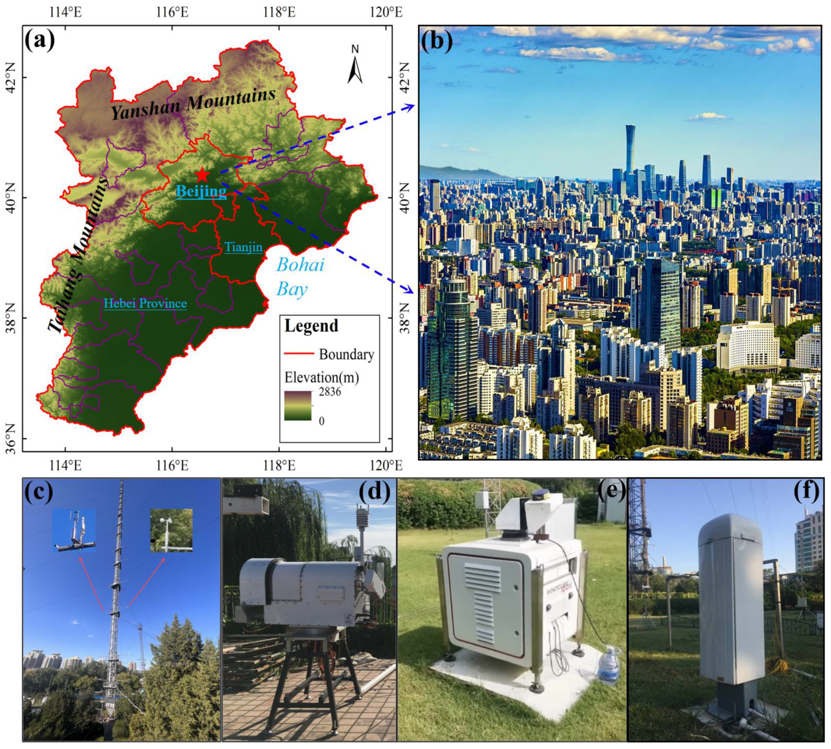
Figure 1. (a) Location of observation stations, (b) Landscape around observation stations, (c) The 325 m tower, (d) the microwave radiometer, (e) the Doppler wind lidar, and (f) the CL51 ceilometer.
Remotesensing 16 01075 g001
Figure 2. Scatter plots of WS measured by the Doppler wind lidar from 1−25 January 2019 versus that of the IAP 325 m tower.
Remotesensing 16 01075 g002
Figure 3. Comparison of horizontal wind vectors observed by the Doppler wind lidar and the 325 m tower at different heights.
Remotesensing 16 01075 g003
Figure 4. Same as Figure 2 but for temperature, T.
Remotesensing 16 01075 g004
Figure 5. Same as Figure 2 but for relative humidity, RH.
Remotesensing 16 01075 g005
Figure 6. The Ri values calculated from the lidar−radiometer and the 325 m tower data at different altitudes.
Remotesensing 16 01075 g006
Figure 7. The horizontal WS (a), vertical WS (b), horizontal WD (c), u−component of the horizontal WS (d), and v−component of the horizontal WS (e) measured by the Doppler wind lidar from 1 to 25 January 2019.
Remotesensing 16 01075 g007
Figure 8. Temperature (a), horizontal WD (b), temperature lapse rate (c), relative humidity (d), and virtual potential temperature lapse rate (e) from 1 to 25 January 2019.
Remotesensing 16 01075 g008
Figure 9. Ri images (ai) from different spatial (25 m, 50 m, 100 m) and temporal resolution (1 min, 30 min, 1 h) datasets for the period 1−25 January 2019.
Remotesensing 16 01075 g009
Figure 10. Taylor diagram of Ri from different spatial and temporal resolution datasets for the period 1–25 January 2019.
Remotesensing 16 01075 g010
Figure 11. The daily average values for Ri, wind field, and boundary layer height for the period 1−25 January 2019.
Remotesensing 16 01075 g011
Disclaimer/Publisher’s Note: The statements, opinions and data contained in all publications are solely those of the individual author(s) and contributor(s) and not of MDPI and/or the editor(s). MDPI and/or the editor(s) disclaim responsibility for any injury to people or property resulting from any ideas, methods, instructions or products referred to in the content.