
Multistage Interaction Network for Remote Sensing Change Detection

Abstract
:1. Introduction
- We introduce a multistage interaction network that allows our network to leverage the advantages of both early fusion and late fusion for effective change extraction;
- We introduce the spatial and channel interactions to overcome challenges posed by background diversity and pseudo-changes;
- Extensive experiments on LEVIR-CD, WHU-CD, and CLCD datasets showcase promising performance with F1 (we provide the definition in Section 3.1), with scores of 91.47%, 93.73%, and 76.60%, respectively.
2. The Proposed Method
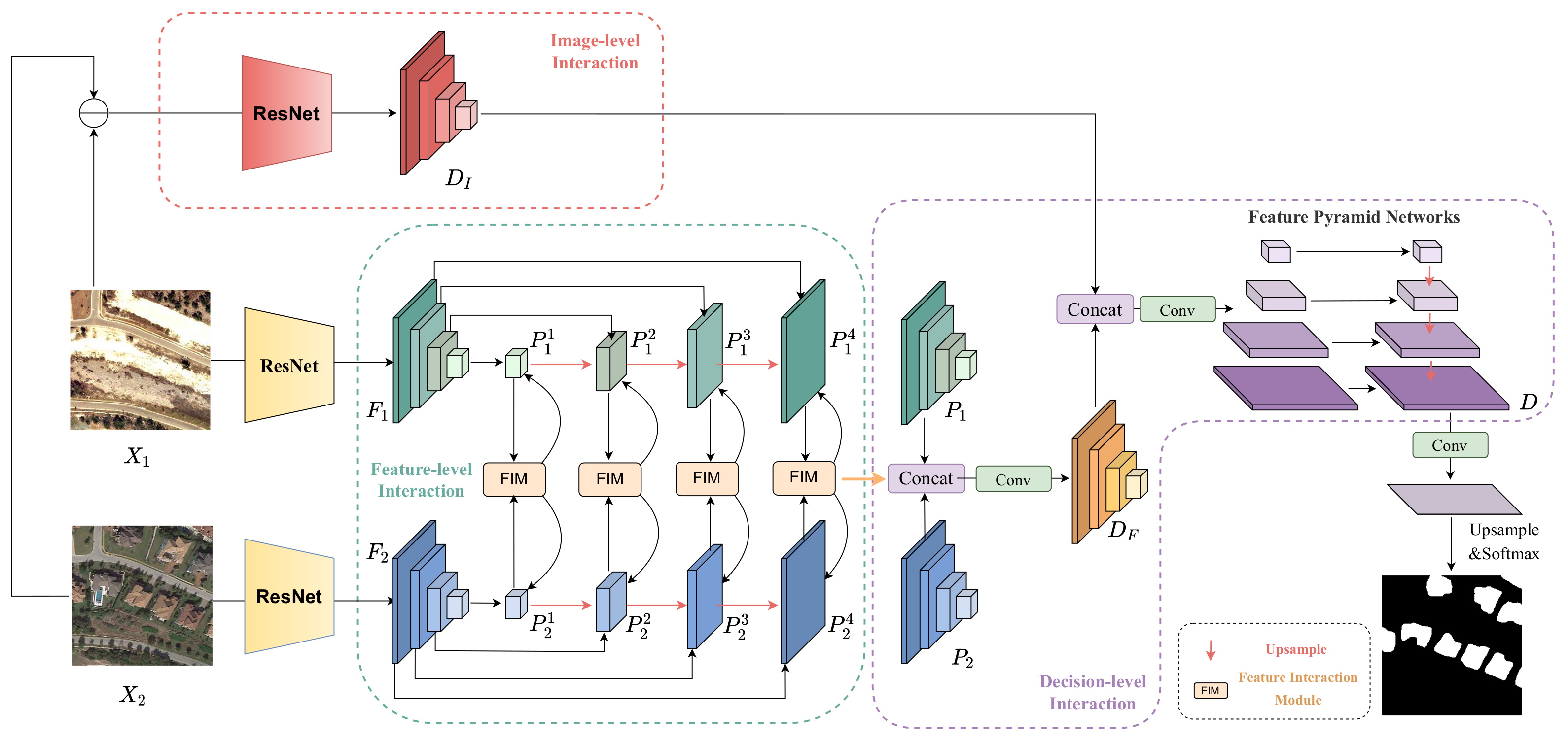
2.1. Overall Framework
2.2. Image-Level Interaction
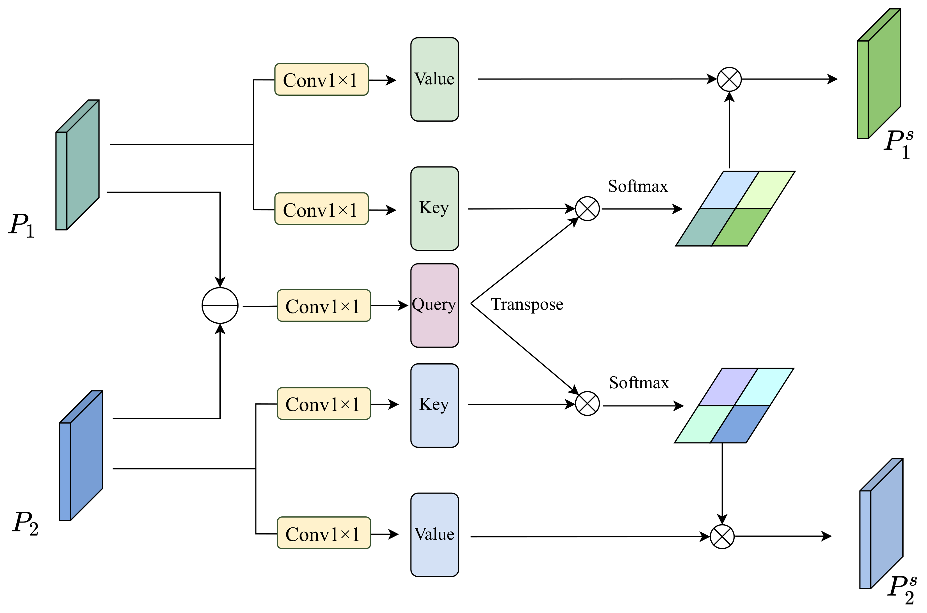
2.3. Feature-Level Interaction
2.4. Decision-Level Interaction
3. Experimental Results
3.1. Experimental Setting
- LEVIR-CD [15] is a large-scale dataset for building change detection, consisting of 637 pairs of high-resolution images from Google Earth. Each image is pixels with a spatial resolution of 0.5 m. The dataset spans 20 different regions from 2002 to 2018. Following [15], images are segmented into non-overlapping patches of pixels, resulting in a total of 7120/1024/2048 samples for training, validation, and testing, respectively;
- WHU-CD [46] is a publicly available building change detection dataset. It comprises one pair of aerial images covering the area of Christchurch, New Zealand, for the years 2012 and 2016. The image dimensions are pixels with a spatial resolution of 0.075 m. Similar to LEVIR-CD, the dataset is divided into non-overlapping patches of pixels. The dataset is randomly split into 6096/762/762 samples for training, validation, and testing, respectively;
- CLCD [47] is a dataset designed for cropland change detection, collected by Gaofen-2 in Guangdong Province, China, in 2017 and 2019. It consists of 600 pairs of cropland change samples, each with dimensions of pixels and varying spatial resolutions from 0.5 to 2 m. Following the methodology in [47], we allocate 360 pairs for training, 120 pairs for validation, and 120 pairs for testing.
- OA calculates the ratio of correctly classified pixels to the total number of pixels in the dataset, defined by
- Precision measures the fraction of detections that were actually changed among all the instances predicted as changed, defined by
- Recall measures the ability of the model to capture all the actual changes, defined by
- F1 combines recall and precision together, defined by
- IoU computes the overlap between the predicted and actual change regions, defined by
3.2. Comparisons with State-of-the-Art
3.2.1. Results on LEVIR-CD Dataset
3.2.2. Results on WHU-CD Dataset
3.2.3. Results on CLCD Dataset
3.3. Ablation Study
3.3.1. Effectiveness of Different Modules
3.3.2. Effectiveness of Spatial and Channel Interaction Blocks
3.4. Discussion
4. Conclusions
Author Contributions
Funding
Data Availability Statement
Conflicts of Interest
References
- Shafique, A.; Cao, G.; Khan, Z.; Asad, M.; Aslam, M. Deep learning-based change detection in remote sensing images: A review. Remote Sens. 2022, 14, 871. [Google Scholar] [CrossRef]
- Jiang, H.; Peng, M.; Zhong, Y.; Xie, H.; Hao, Z.; Lin, J.; Ma, X.; Hu, X. A survey on deep learning-based change detection from high-resolution remote sensing images. Remote Sens. 2022, 14, 1552. [Google Scholar] [CrossRef]
- Bruzzone, L.; Prieto, D. Automatic analysis of the difference image for unsupervised change detection. IEEE Trans. Geosci. Remote Sens. 2000, 38, 1171–1182. [Google Scholar] [CrossRef]
- Du, B.; Wang, Y.; Wu, C.; Zhang, L. Unsupervised scene change detection via latent Dirichlet allocation and multivariate alteration detection. IEEE J. Sel. Top. Appl. Earth Observ. Remote Sens. 2018, 11, 4676–4689. [Google Scholar] [CrossRef]
- Deng, J.; Wang, K.; Deng, Y.; Qi, G. PCA-based land-use change detection and analysis using multitemporal and multisensor satellite data. Int. J. Remote Sens. 2008, 29, 4823–4838. [Google Scholar] [CrossRef]
- Shi, W.; Zhang, M.; Zhang, R.; Chen, S.; Zhan, Z. Change detection based on artificial intelligence: State-of-the-art and challenges. Remote Sens. 2020, 12, 1688. [Google Scholar] [CrossRef]
- Jaturapitpornchai, R.; Matsuoka, M.; Kanemoto, N.; Kuzuoka, S.; Ito, R.; Nakamura, R. Newly built construction detection in SAR images using deep learning. Remote Sens. 2019, 11, 1444. [Google Scholar] [CrossRef]
- Li, Y.; Peng, C.; Chen, Y.; Jiao, L.; Zhou, L.; Shang, R. A Deep Learning Method for Change Detection in Synthetic Aperture Radar Images. IEEE Trans. Geosci. Remote Sens. 2019, 57, 5751–5763. [Google Scholar] [CrossRef]
- Liu, J.; Gong, M.; Qin, K.; Zhang, P. A Deep Convolutional Coupling Network for Change Detection Based on Heterogeneous Optical and Radar Images. IEEE Trans. Neural Netw. Learn. Syst. 2018, 29, 545–559. [Google Scholar] [CrossRef]
- Zhang, P.; Gong, M.; Su, L.; Liu, J.; Li, Z. Change detection based on deep feature representation and mapping transformation for multi-spatial-resolution remote sensing images. ISPRS J. Photogramm. Remote Sens. 2016, 116, 24–41. [Google Scholar] [CrossRef]
- Daudt, R.C.; Le Saux, B.; Boulch, A. Fully convolutional siamese networks for change detection. In Proceedings of the IEEE International Conference on Image Processing (ICIP), Athens, Greece, 7–10 October 2018; pp. 4063–4067. [Google Scholar]
- Wang, M.; Tan, K.; Jia, X.; Wang, X.; Chen, Y. A deep siamese network with hybrid convolutional feature extraction module for change detection based on multi-sensor remote sensing images. Remote Sens. 2020, 12, 205. [Google Scholar] [CrossRef]
- Wu, J.; Xie, C.; Zhang, Z.; Zhu, Y. A deeply supervised attentive high-resolution network for change detection in remote sensing images. Remote Sens. 2022, 15, 45. [Google Scholar] [CrossRef]
- Xiong, F.; Li, T.; Chen, J.; Zhou, J.; Qian, Y. Mask-Guided Local–Global Attentive Network for Change Detection in Remote Sensing Images. IEEE J. Sel. Top. Appl. Earth Observ. Remote Sens. 2024, 17, 3366–3378. [Google Scholar] [CrossRef]
- Chen, H.; Shi, Z. A spatial-temporal attention-based method and a new dataset for remote sensing image change detection. Remote Sens. 2020, 12, 1662. [Google Scholar] [CrossRef]
- Song, K.; Jiang, J. AGCDetNet:An Attention-Guided Network for Building Change Detection in High-Resolution Remote Sensing Images. IEEE J. Sel. Top. Appl. Earth Observ. Remote Sens. 2021, 14, 4816–4831. [Google Scholar] [CrossRef]
- Peng, X.; Zhong, R.; Li, Z.; Li, Q. Optical Remote Sensing Image Change Detection Based on Attention Mechanism and Image Difference. IEEE Trans. Geosci. Remote Sens. 2021, 59, 7296–7307. [Google Scholar] [CrossRef]
- Shi, Q.; Liu, M.; Li, S.; Liu, X.; Wang, F.; Zhang, L. A Deeply Supervised Attention Metric-Based Network and an Open Aerial Image Dataset for Remote Sensing Change Detection. IEEE Trans. Geosci. Remote Sens. 2022, 60, 5604816. [Google Scholar] [CrossRef]
- Liu, M.; Huang, J.; Ma, L.; Wan, L.; Guo, J.; Yao, D. A Spatial-Temporal-Channel Attention Unet++ for High Resolution Remote Sensing Image Change Detection. In Proceedings of the IEEE International Geoscience and Remote Sensing Symposium (IGARSS), Brussels, Belgium, 11–16 July 2021; pp. 4344–4347. [Google Scholar]
- Eftekhari, A.; Samadzadegan, F.; Javan, F.D. Building change detection using the parallel spatial-channel attention block and edge-guided deep network. Int. J. Appl. Earth Obs. Geoinf. 2023, 117, 103180. [Google Scholar] [CrossRef]
- Wang, D.; Chen, X.; Jiang, M.; Du, S.; Xu, B.; Wang, J. ADS-Net: An Attention-Based deeply supervised network for remote sensing image change detection. Int. J. Appl. Earth Obs. Geoinf. 2021, 101, 102348. [Google Scholar]
- Li, Z.; Tang, C.; Liu, X.; Zhang, W.; Dou, J.; Wang, L.; Zomaya, A.Y. Lightweight Remote Sensing Change Detection with Progressive Feature Aggregation and Supervised Attention. IEEE Trans. Geosci. Remote Sens. 2023, 61, 5602812. [Google Scholar] [CrossRef]
- Chen, H.; Qi, Z.; Shi, Z. Remote sensing image change detection with transformers. IEEE Trans. Geosci. Remote Sens. 2021, 60, 5607514. [Google Scholar] [CrossRef]
- Zhang, C.; Wang, L.; Cheng, S.; Li, Y. SwinSUNet: Pure Transformer Network for Remote Sensing Image Change Detection. IEEE Trans. Geosci. Remote Sens. 2022, 60, 1–13. [Google Scholar] [CrossRef]
- Zheng, Z.; Zhong, Y.; Tian, S.; Ma, A.; Zhang, L. ChangeMask: Deep multi-task encoder-transformer-decoder architecture for semantic change detection. ISPRS J. Photogramm. Remote Sens. 2022, 183, 228–239. [Google Scholar] [CrossRef]
- Tang, X.; Zhang, T.; Ma, J.; Zhang, X.; Liu, F.; Jiao, L. WNet: W-Shaped Hierarchical Network for Remote-Sensing Image Change Detection. IEEE Trans. Geosci. Remote Sens. 2023, 61, 5615814. [Google Scholar] [CrossRef]
- Li, Q.; Zhong, R.; Du, X.; Du, Y. TransUNetCD: A Hybrid Transformer Network for Change Detection in Optical Remote-Sensing Images. IEEE Trans. Geosci. Remote Sens. 2022, 60, 5622519. [Google Scholar] [CrossRef]
- Bai, B.; Fu, W.; Lu, T.; Li, S. Edge-Guided Recurrent Convolutional Neural Network for Multitemporal Remote Sensing Image Building Change Detection. IEEE Trans. Geosci. Remote Sens. 2022, 60, 5610613. [Google Scholar] [CrossRef]
- Ding, L.; Zhu, K.; Peng, D.; Tang, H.; Yang, K.; Bruzzone, L. Adapting Segment Anything Model for Change Detection in VHR Remote Sensing Images. IEEE Trans. Geosci. Remote Sens. 2024, 62, 5611711. [Google Scholar] [CrossRef]
- Feng, Y.; Xu, H.; Jiang, J.; Liu, H.; Zheng, J. ICIF-Net: Intra-Scale Cross-Interaction and Inter-Scale Feature Fusion Network for Bitemporal Remote Sensing Images Change Detection. IEEE Trans. Geosci. Remote Sens. 2022, 60, 1–13. [Google Scholar] [CrossRef]
- Liang, S.; Hua, Z.; Li, J. Enhanced Feature Interaction Network for Remote Sensing Change Detection. IEEE Geosci. Remote Sens. Lett. 2023, 20, 1–5. [Google Scholar] [CrossRef]
- Feng, Y.; Jiang, J.; Xu, H.; Zheng, J. Change Detection on Remote Sensing Images Using Dual-Branch Multilevel Intertemporal Network. IEEE Trans. Geosci. Remote Sens. 2023, 61, 3241257. [Google Scholar] [CrossRef]
- Zhang, C.; Yue, P.; Tapete, D.; Jiang, L.; Shangguan, B.; Huang, L.; Liu, G. A deeply supervised image fusion network for change detection in high resolution bi-temporal remote sensing images. ISPRS J. Photogramm. Remote Sens. 2020, 166, 183–200. [Google Scholar] [CrossRef]
- Zhang, M.; Shi, W. A feature difference convolutional neural network-based change detection method. IEEE Trans. Geosci. Remote Sens. 2020, 58, 7232–7246. [Google Scholar] [CrossRef]
- Xiang, S.; Wang, M.; Jiang, X.; Xie, G.; Zhang, Z.; Tang, P. Dual-task semantic change detection for remote sensing images using the generative change field module. Remote Sens. 2021, 13, 3336. [Google Scholar] [CrossRef]
- Zheng, Z.; Wan, Y.; Zhang, Y.; Xiang, S.; Peng, D.; Zhang, B. CLNet: Cross-layer convolutional neural network for change detection in optical remote sensing imagery. ISPRS J. Photogramm. Remote Sens. 2021, 175, 247–267. [Google Scholar] [CrossRef]
- Ma, H.; Zhao, L.; Li, B.; Niu, R.; Wang, Y. Change Detection Needs Neighborhood Interaction in Transformer. Remote Sens. 2023, 15, 5459. [Google Scholar] [CrossRef]
- Lyu, H.; Lu, H.; Mou, L. Learning a transferable change rule from a recurrent neural network for land cover change detection. Remote Sens. 2016, 8, 506. [Google Scholar] [CrossRef]
- Mou, L.; Bruzzone, L.; Zhu, X.X. Learning spectral-spatial-temporal features via a recurrent convolutional neural network for change detection in multispectral imagery. IEEE Trans. Geosci. Remote Sens. 2018, 57, 924–935. [Google Scholar] [CrossRef]
- Song, A.; Choi, J.; Han, Y.; Kim, Y. Change detection in hyperspectral images using recurrent 3D fully convolutional networks. Remote Sens. 2018, 10, 1827. [Google Scholar] [CrossRef]
- Zheng, J.; Tian, Y.; Yuan, C.; Yin, K.; Zhang, F.; Chen, F.; Chen, Q. MDESNet: Multitask Difference-Enhanced Siamese Network for Building Change Detection in High-Resolution Remote Sensing Images. Remote Sens. 2022, 14, 3775. [Google Scholar] [CrossRef]
- Zhang, L.; Hu, X.; Zhang, M.; Shu, Z.; Zhou, H. Object-level change detection with a dual correlation attention-guided detector. ISPRS J. Photogramm. Remote Sens. 2021, 177, 147–160. [Google Scholar] [CrossRef]
- Cheng, G.; Wang, G.; Han, J. ISNet: Towards Improving Separability for Remote Sensing Image Change Detection. IEEE Trans. Geosci. Remote Sens. 2022, 60, 5623811. [Google Scholar] [CrossRef]
- Fang, S.; Li, K.; Li, Z. Changer: Feature Interaction is What You Need for Change Detection. IEEE Trans. Geosci. Remote Sens. 2023, 61, 5610111. [Google Scholar] [CrossRef]
- Wang, Y.; Huang, W.; Sun, F.; Xu, T.; Rong, Y.; Huang, J. Deep multimodal fusion by channel exchanging. In Proceedings of the 34th Conference on Neural Information Processing Systems (NeurIPS 2020), Vancouver, BC, Canada, 6–12 December 2020; pp. 4835–4845. [Google Scholar]
- Ji, S.; Wei, S.; Lu, M. Fully Convolutional Networks for Multisource Building Extraction From an Open Aerial and Satellite Imagery Data Set. IEEE Trans. Geosci. Remote Sens. 2019, 57, 574–586. [Google Scholar] [CrossRef]
- Liu, M.; Chai, Z.; Deng, H.; Liu, R. A CNN-transformer network with multiscale context aggregation for fine-grained cropland change detection. IEEE J. Sel. Top. Appl. Earth Observ. Remote Sens. 2022, 15, 4297–4306. [Google Scholar] [CrossRef]
- Liu, Y.; Pang, C.; Zhan, Z.; Zhang, X.; Yang, X. Building change detection for remote sensing images using a dual-task constrained deep siamese convolutional network model. IEEE Geosci. Remote Sens. Lett. 2020, 18, 811–815. [Google Scholar] [CrossRef]
- Bandara, W.G.C.; Patel, V.M. A transformer-based siamese network for change detection. In Proceedings of the IEEE International Geoscience and Remote Sensing Symposium, Kuala Lumpur, Malaysia, 17–22 July 2022; pp. 207–210. [Google Scholar]


| Method | Architecture | Interaction | Params | FLOPs |
|---|---|---|---|---|
| FC-EF | CNN | Image-level | 1.351 M | 3.577 G |
| FC-Siam-Diff | CNN | Feature-level | 1.350 M | 4.727 G |
| FC-Siam-Conc | CNN | Feature-level | 1.546 M | 5.331 G |
| STANet | CNN | Feature-level | 16.892 M | 26.022 G |
| DTCDSCN | CNN | Feature-level | 31.257 M | 13.224 G |
| ChangeFormer | Transformer | Feature-level | 41.027 M | 202.788 G |
| BIT | Transformer | Feature-level | 3.496 M | 10.633 G |
| ICIF-Net | Transformer+CNN | Feature-level | 23.843 M | 25.410 G |
| DMINet | CNN | Feature-level | 6.242 M | 14.551 G |
| WNet | Transformer+CNN | Feature-level | 43.07 M | 19.20 G |
| MIN-Net (Ours) | CNN | Multistage | 42.12 M | 15.37 G |
| Method | P | R | F1 | IoU | OA |
|---|---|---|---|---|---|
| FC-EF [11] | 86.91 | 80.17 | 83.40 | 71.53 | 98.39 |
| FC-Siam-Diff [11] | 89.53 | 83.31 | 86.31 | 75.92 | 98.67 |
| FC-Siam-Conc [11] | 91.99 | 76.77 | 83.69 | 71.96 | 98.49 |
| STANet [15] | 83.81 | 91.00 | 87.26 | 77.40 | 98.66 |
| DTCDSCN [48] | 88.53 | 86.83 | 87.67 | 78.05 | 98.77 |
| ChangeFormer [49] | 92.05 | 88.80 | 90.40 | 82.48 | 99.04 |
| BIT [23] | 89.24 | 89.37 | 89.31 | 80.68 | 98.92 |
| ICIF-Net [30] | 91.39 | 89.24 | 90.38 | 82.31 | 98.99 |
| DMINet [32] | 92.52 | 88.86 | 90.70 | 82.99 | 99.07 |
| WNet [26] | 91.23 | 89.62 | 90.42 | 82.51 | 99.03 |
| MIN-Net (Ours) | 92.04 | 90.91 | 91.47 | 84.29 | 99.14 |
| Method | P | R | F1 | IoU | OA |
|---|---|---|---|---|---|
| FC-EF [11] | 83.54 | 73.85 | 78.39 | 64.47 | 98.21 |
| FC-Siam-Diff [11] | 85.92 | 78.89 | 82.26 | 69.86 | 98.50 |
| FC-Siam-Conc [11] | 82.46 | 85.24 | 83.83 | 72.16 | 98.55 |
| STANet [15] | 85.10 | 79.40 | 82.20 | 69.70 | 98.50 |
| DTCDSCN [48] | 91.42 | 87.60 | 89.47 | 80.94 | 99.09 |
| ChangeFormer [49] | 92.06 | 83.46 | 87.55 | 77.86 | 98.96 |
| BIT [23] | 93.91 | 87.84 | 90.78 | 83.11 | 99.21 |
| ICIF-Net [30] | 91.19 | 85.92 | 88.48 | 79.34 | 99.01 |
| DMINet [32] | 82.87 | 87.54 | 85.14 | 74.12 | 98.65 |
| WNet [26] | 94.17 | 83.94 | 88.76 | 79.79 | 99.06 |
| MIN-Net (Ours) | 95.26 | 92.25 | 93.73 | 88.20 | 99.46 |
| Method | P | R | F1 | IoU | OA |
|---|---|---|---|---|---|
| FC-EF [11] | 58.88 | 56.32 | 57.57 | 40.42 | 93.82 |
| FC-Siam-Diff [11] | 59.27 | 62.38 | 60.79 | 43,66 | 94.31 |
| FC-Siam-Conc [11] | 61.71 | 65.29 | 63.00 | 45.99 | 94.85 |
| STANet [15] | 55.80 | 68.00 | 61.30 | 38.40 | 93.60 |
| DTCDSCN [48] | 61.25 | 59.11 | 60.16 | 43.02 | 94.18 |
| ChangeFormer [49] | 58.29 | 47.25 | 52.19 | 35.31 | 93.56 |
| BIT [23] | 64.18 | 58.63 | 61.28 | 44.18 | 94.48 |
| ICIF-Net [30] | 66.84 | 54.02 | 58.75 | 42.60 | 94.58 |
| DMINet [32] | 70.30 | 46.40 | 55.90 | 38.79 | 94.55 |
| WNet [26] | 68.45 | 57.82 | 62.69 | 45.66 | 94.88 |
| MIN-Net (Ours) | 77.53 | 75.70 | 76.60 | 62.08 | 96.56 |
| Dataset | Method | P | R | F1 | IoU | OA |
|---|---|---|---|---|---|---|
| LEVIR-CD | BaseLine | 90.82 | 90.80 | 90.81 | 83.16 | 99.06 |
| w/Image | 92.17 | 90.04 | 91.09 | 83.64 | 99.10 | |
| w/Feature | 91.81 | 90.82 | 91.32 | 84.02 | 99.12 | |
| Ours | 92.04 | 90.91 | 91.47 | 84.29 | 99.14 | |
| WHU-CD | BaseLine | 95.02 | 90.23 | 92.57 | 86.16 | 99.36 |
| w/Image | 94.72 | 92.21 | 93.45 | 87.70 | 99.43 | |
| w/Feature | 95.26 | 91.64 | 93.41 | 87.64 | 99.43 | |
| Ours | 95.26 | 92.25 | 93.73 | 88.20 | 99.46 | |
| CLCD | BaseLine | 75.06 | 74.45 | 74.75 | 59.69 | 96.26 |
| w/Image | 76.20 | 74.91 | 75.54 | 60.70 | 96.39 | |
| w/Feature | 78.12 | 73.48 | 75.73 | 60.94 | 96.50 | |
| Ours | 77.52 | 75.70 | 76.60 | 62.08 | 96.56 |
| Dataset | Method | P | R | F1 | IoU | OA |
|---|---|---|---|---|---|---|
| LEVIR-CD | w/o spatial | 92.01 | 90.20 | 91.10 | 83.65 | 99.10 |
| w/o channel | 91.60 | 90.66 | 91.13 | 83.70 | 99.10 | |
| Ours | 91.81 | 90.82 | 91.32 | 84.02 | 99.12 | |
| WHU-CD | w/o spatial | 94.65 | 91.54 | 93.07 | 87.04 | 99.40 |
| w/o channel | 94.73 | 91.15 | 92.90 | 86.75 | 99.39 | |
| Ours | 95.26 | 91.64 | 93.41 | 87.64 | 99.43 | |
| CLCD | w/o spatial | 80.38 | 70.77 | 75.27 | 60.35 | 96.54 |
| w/o channel | 78.36 | 72.77 | 75.46 | 60.59 | 96.48 | |
| Ours | 78.12 | 73.48 | 75.73 | 60.94 | 96.50 |
Disclaimer/Publisher’s Note: The statements, opinions and data contained in all publications are solely those of the individual author(s) and contributor(s) and not of MDPI and/or the editor(s). MDPI and/or the editor(s) disclaim responsibility for any injury to people or property resulting from any ideas, methods, instructions or products referred to in the content. |
© 2024 by the authors. Licensee MDPI, Basel, Switzerland. This article is an open access article distributed under the terms and conditions of the Creative Commons Attribution (CC BY) license (https://creativecommons.org/licenses/by/4.0/).
Share and Cite
Zhou, M.; Qian, W.; Ren, K. Multistage Interaction Network for Remote Sensing Change Detection. Remote Sens. 2024, 16, 1077. https://doi.org/10.3390/rs16061077
Zhou M, Qian W, Ren K. Multistage Interaction Network for Remote Sensing Change Detection. Remote Sensing. 2024; 16(6):1077. https://doi.org/10.3390/rs16061077
Chicago/Turabian StyleZhou, Meng, Weixian Qian, and Kan Ren. 2024. "Multistage Interaction Network for Remote Sensing Change Detection" Remote Sensing 16, no. 6: 1077. https://doi.org/10.3390/rs16061077
APA StyleZhou, M., Qian, W., & Ren, K. (2024). Multistage Interaction Network for Remote Sensing Change Detection. Remote Sensing, 16(6), 1077. https://doi.org/10.3390/rs16061077