
Characterizing the Accelerated Global Carbon Emissions from Forest Loss during 1985–2020 Using Fine-Resolution Remote Sensing Datasets


Abstract
1. Introduction
2. Materials and Methods
2.1. Materials
2.1.1. Global Land Cover Dataset
2.1.2. Global Biomass Datasets
2.1.3. Global SOC Dataset
2.1.4. Other Data
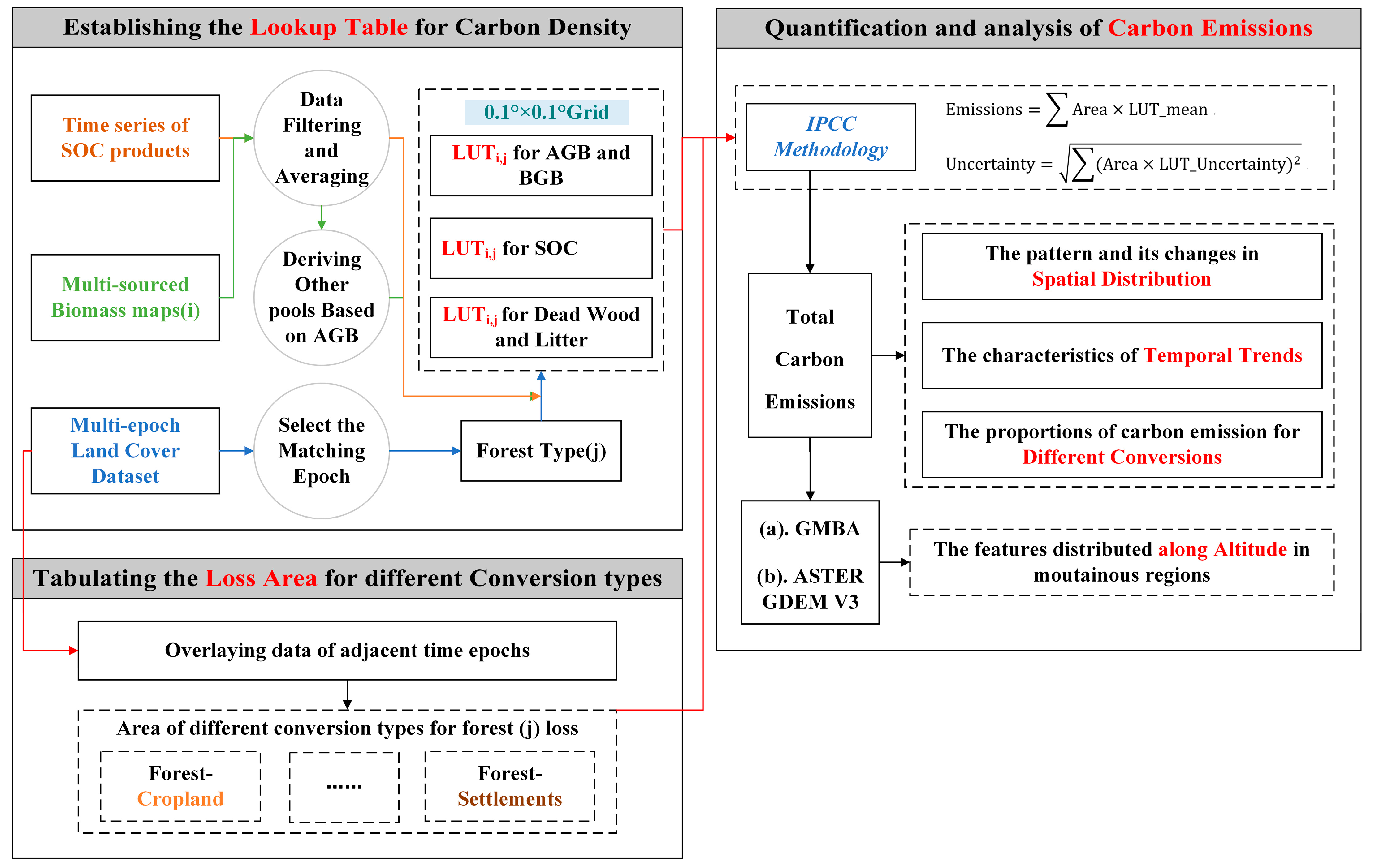
2.2. Methods
2.2.1. Establishing the LUT of Carbon Density
2.2.2. Assessing the Area of Forest Converted to other Land Cover Categories
2.2.3. Quantifying Carbon Emissions Due to Forest Loss and Associated Uncertainties
2.2.4. Determining the Variation in Carbon Emissions with Altitude in Mountainous Regions
3. Results
3.1. Characteristics of Global Forest Loss over the Past 35 Years
3.2. Patterns of Global Carbon Emissions during the Period 1985–2020
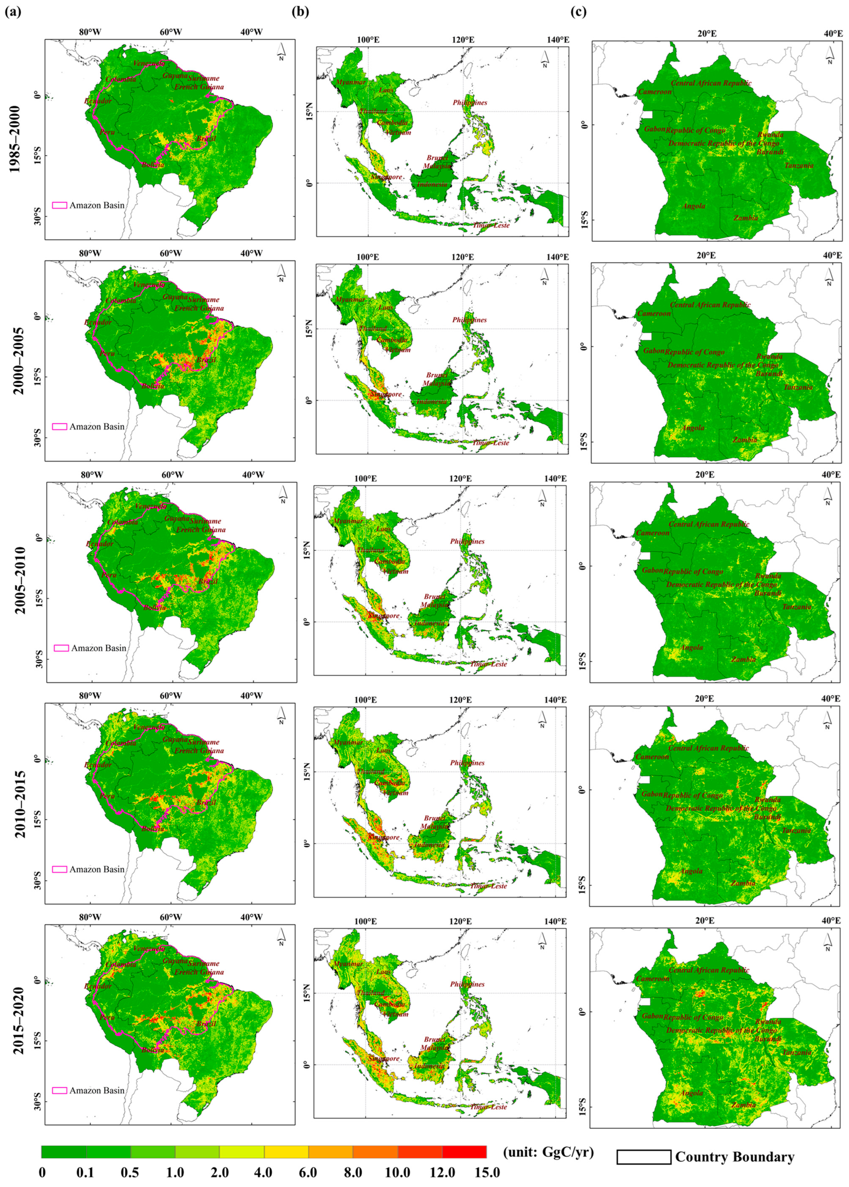
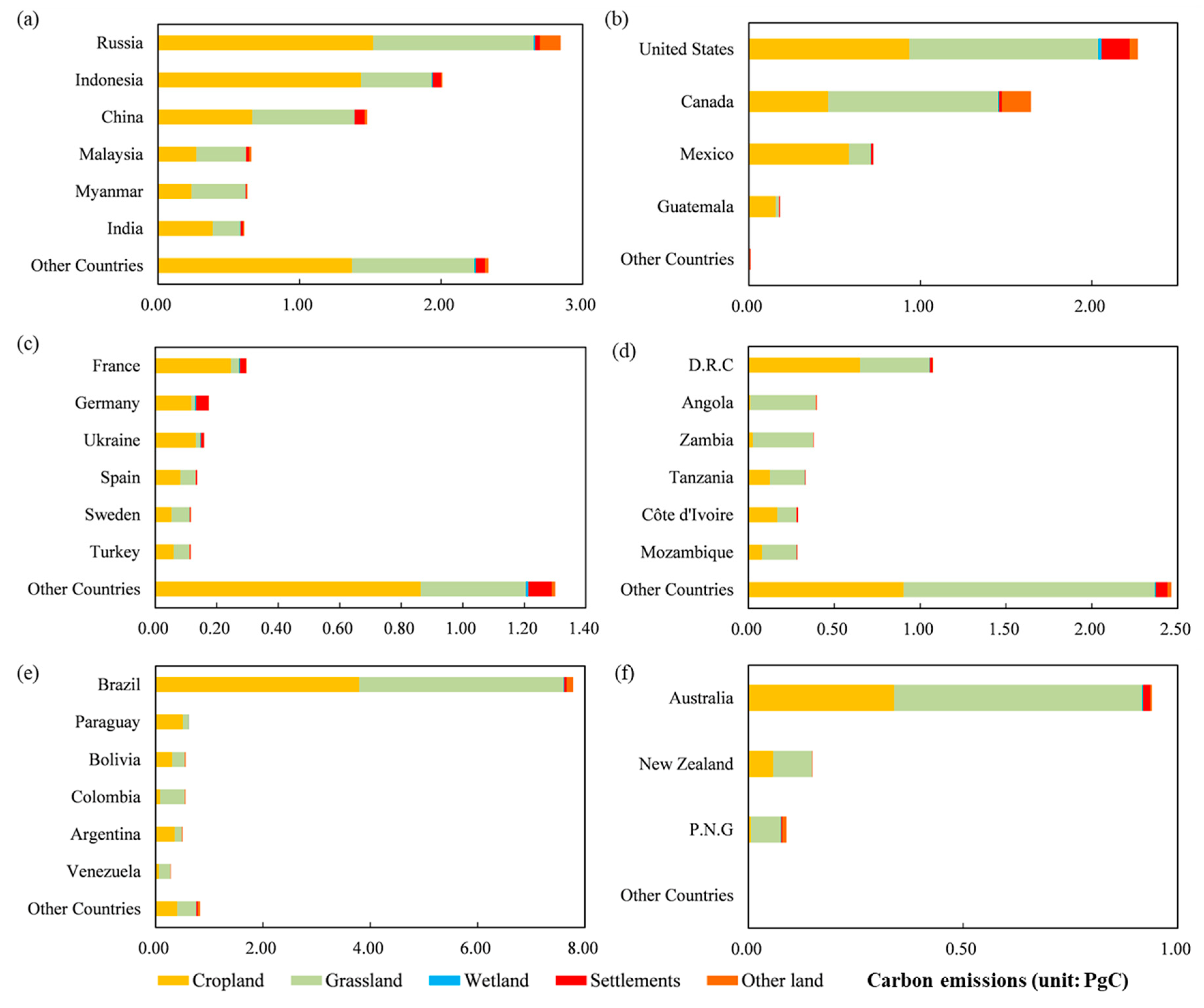
3.2.1. Spatial Distribution of Global Carbon Emissions
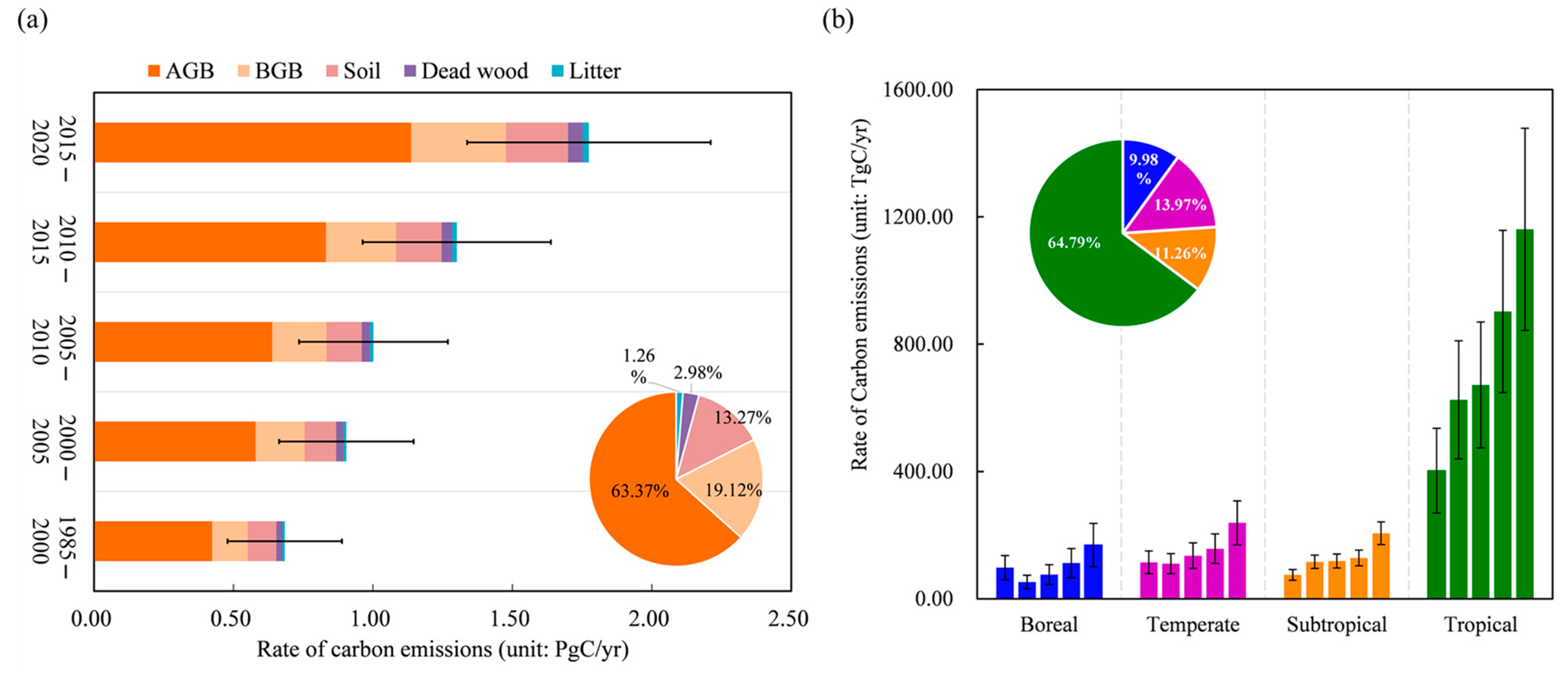
3.2.2. Temporal Trends in Global Carbon Emissions
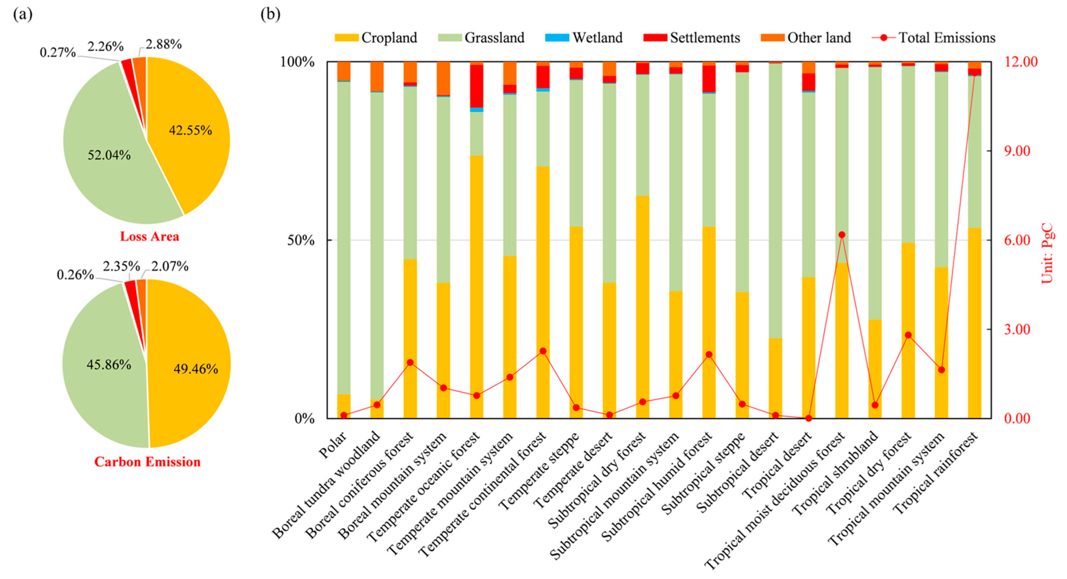
3.3. Contributions of Various Forest Conversion Types to Global Carbon Emissions
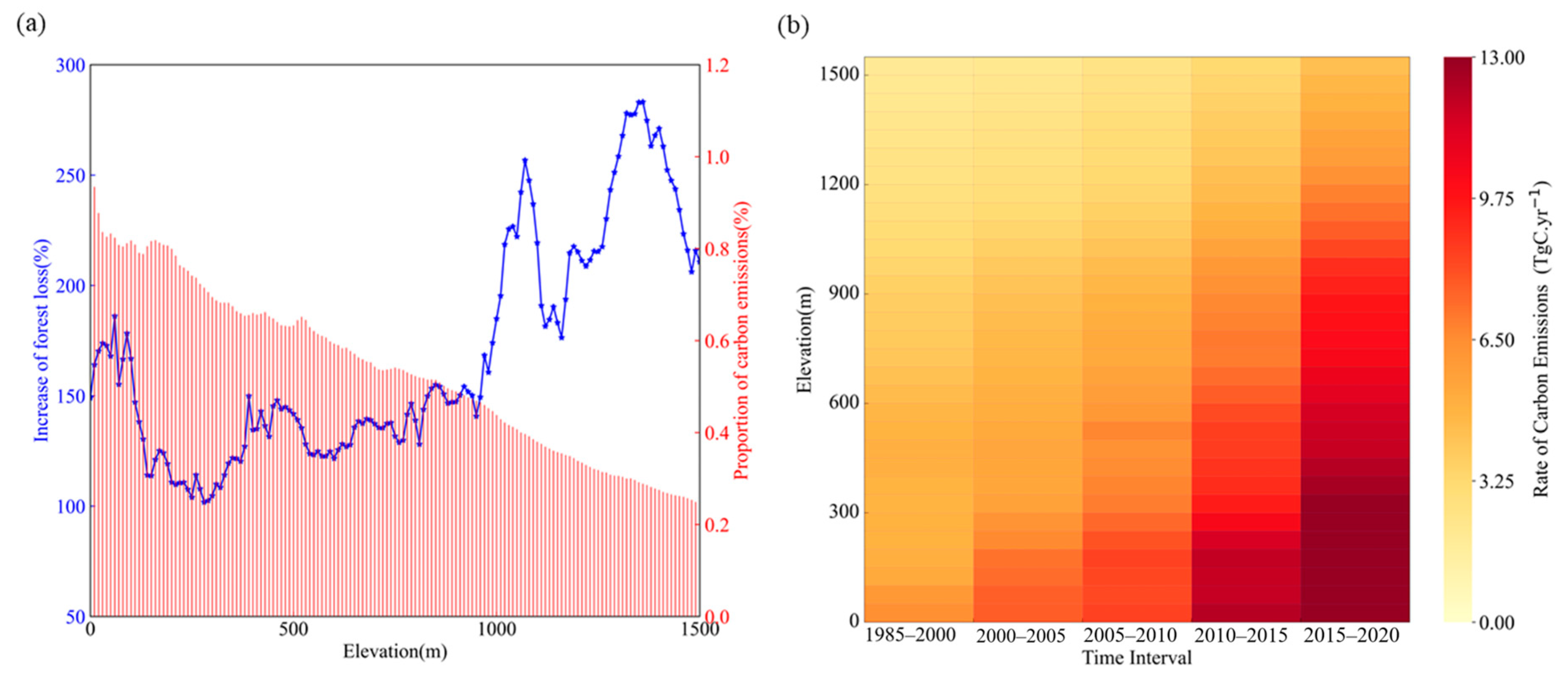
3.4. Trends of Carbon Emissions in Mountainous Regions during 1985–2020
4. Discussion
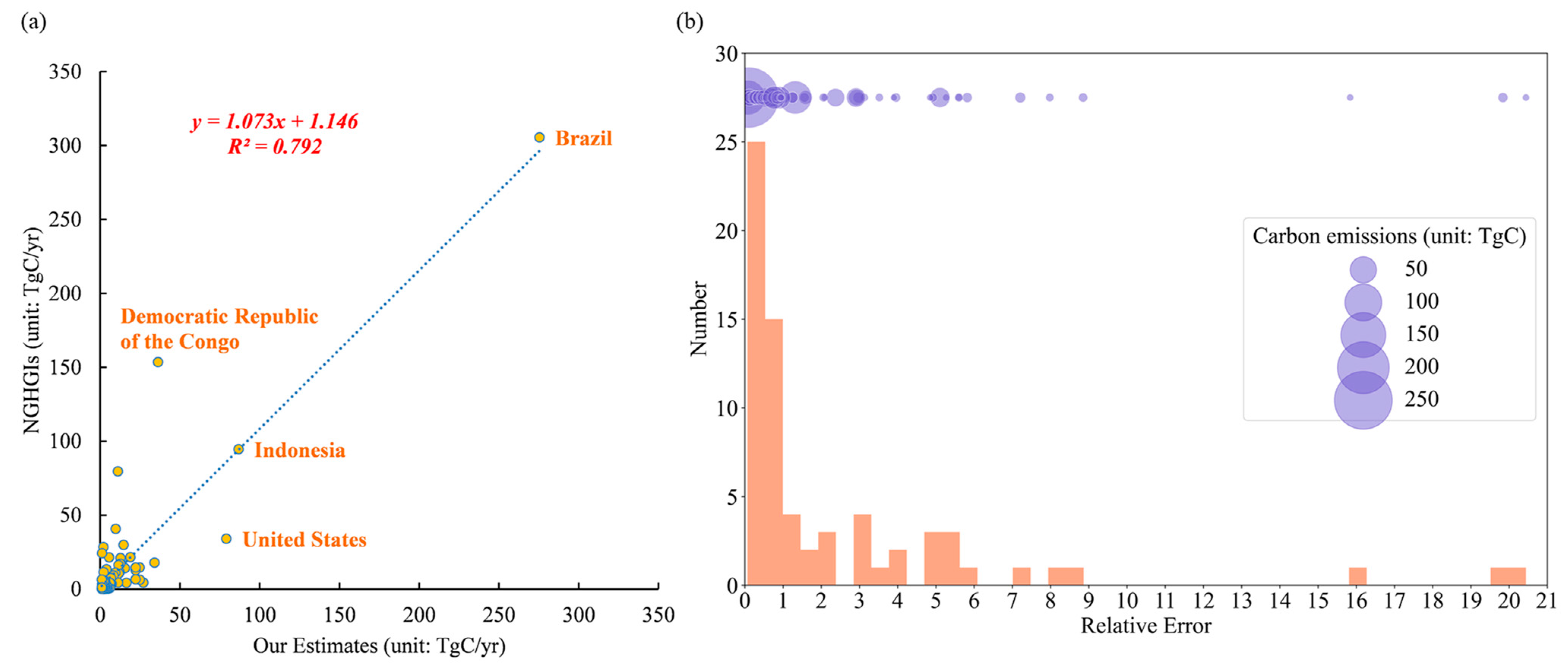
4.1. Comparisons with Previous Estimations
4.2. Limitations and Uncertainties
4.3. Implications for Slowing Global Carbon Emissions from Forest Loss
5. Conclusions
Author Contributions
Funding
Data Availability Statement
Acknowledgments
Conflicts of Interest
Appendix A

| Fine-Resolution Classification System | Land Cover Code | IPCC Category | Percentage of SOC Emissions |
|---|---|---|---|
| Rainfed cropland | 10 | Cropland | 20% |
| Herbaceous cover | 11 | ||
| Tree or shrub cover (Orchard) | 12 | ||
| Irrigated cropland | 20 | ||
| Open evergreen broad-leaved forest | 51 | Forest land | 0% |
| Closed evergreen broad-leaved forest | 52 | ||
| Open deciduous broad-leaved forest (0.15 < fc < 0.4) | 61 | ||
| Closed deciduous broad-leaved forest (fc > 0.4) | 62 | ||
| Open evergreen needle-leaved forest (0.15 < fc < 0.4) | 71 | ||
| Closed evergreen needle-leaved forest (fc > 0.4) | 72 | ||
| Open deciduous needle-leaved forest (0.15 < fc < 0.4) | 81 | ||
| Closed deciduous needle-leaved forest (fc > 0.4) | 82 | ||
| Open mixed leaf forest (broad-leaved and needle-leaved) | 91 | ||
| Closed mixed leaf forest (broad-leaved and needle-leaved) | 92 | ||
| Shrubland | 120 | Grassland | 11% |
| Evergreen shrubland | 121 | ||
| Deciduous shrubland | 122 | ||
| Grassland | 130 | ||
| Lichens and mosses | 140 | ||
| Sparse vegetation (fc < 0.15) | 150 | ||
| Sparse shrubland (fc < 0.15) | 152 | ||
| Sparse herbaceous (fc < 0.15) | 153 | ||
| Swamp | 181 | Wetlands | 5% |
| Marsh | 182 | ||
| Flooded flat | 183 | ||
| Saline | 184 | ||
| Mangrove | 185 | ||
| Salt marsh | 186 | ||
| Tidal flat | 187 | ||
| Impervious surfaces | 190 | Settlements | 20% |
| Bare areas | 200 | Other land | 5% |
| Consolidated bare areas | 201 | ||
| Unconsolidated bare areas | 202 | ||
| Permanent ice and snow | 220 | ||
| Water body | 210 |
| Code | Name | Climate Zone | Ratio of Dead Wood to AGB | Ratio of Litter to AGB |
|---|---|---|---|---|
| 1 | Polar | Boreal | 8% | 4% |
| 2 | Boreal tundra woodland | 8% | 4% | |
| 3 | Boreal coniferous forest | 8% | 4% | |
| 4 | Boreal mountain system | 8% | 4% | |
| 5 | Water | - | - | |
| 6 | Temperate oceanic forest | Temperate | 8% | 4% |
| 7 | Temperate mountain system | 8% | 4% | |
| 8 | Temperate continental forest | 8% | 4% | |
| 9 | Temperate steppe | 8% | 4% | |
| 10 | Temperate desert | 8% | 4% | |
| 11 | Subtropical dry forest | Subtropical | 2% | 4% |
| 12 | Subtropical mountain system | 7% | 1% | |
| 13 | Subtropical humid forest | 1% | 1% | |
| 14 | Subtropical steppe | 2% | 4% | |
| 15 | Subtropical desert | 2% | 4% | |
| 16 | Tropical desert | Tropical | 2% | 4% |
| 17 | Tropical moist deciduous forest | 1% | 1% | |
| 18 | Tropical shrubland | 2% | 4% | |
| 19 | Tropical dry forest | 2% | 4% | |
| 20 | Tropical mountain system | 7% | 1% | |
| 21 | Tropical rainforest | 6% | 1% |
References
- FAO. Global Forest Resources Assessment 2020: Main Report; Food and Agriculture Organization of the United Nations: Rome, Italy, 2020. [Google Scholar] [CrossRef]
- Winkler, K.; Fuchs, R.; Rounsevell, M.; Herold, M. Global land use changes are four times greater than previously estimated. Nat. Commun. 2021, 12, 2501. [Google Scholar] [CrossRef] [PubMed]
- Avissar, R.; Werth, D. Global Hydroclimatological Teleconnections Resulting from Tropical Deforestation. J. Hydrometeorol. 2005, 6, 134–145. [Google Scholar] [CrossRef]
- Harris, N.L.; Brown, S.; Hagen, S.C.; Saatchi, S.S.; Petrova, S.; Salas, W.; Hansen, M.C.; Potapov, P.V.; Lotsch, A. Baseline map of carbon emissions from deforestation in tropical regions. Science 2012, 336, 1573–1576. [Google Scholar] [CrossRef] [PubMed]
- Friedlingstein, P.; O’Sullivan, M.; Jones, M.W.; Andrew, R.M.; Bakker, D.C.E.; Hauck, J.; Landschützer, P.; Le Quéré, C.; Luijkx, I.T.; Peters, G.P.; et al. Global Carbon Budget 2023. Earth Syst. Sci. Data 2023, 15, 5301–5369. [Google Scholar] [CrossRef]
- Houghton, R.A. Revised estimates of the annual net flux of carbon to the atmosphere from changes in land use and land management 1850–2000. Tellus B Chem. Phys. Meteorol. 2003, 55, 378–390. [Google Scholar]
- Bullock, E.L.; Woodcock, C.E. Carbon loss and removal due to forest disturbance and regeneration in the Amazon. Sci. Total Environ. 2021, 764, 142839. [Google Scholar] [CrossRef]
- Tang, X.; Woodcock, C.E.; Olofsson, P.; Hutyra, L.R. Spatiotemporal assessment of land use/land cover change and associated carbon emissions and uptake in the Mekong River Basin. Remote Sens. Environ. 2021, 256, 112336. [Google Scholar] [CrossRef]
- Houghton, R.A.; House, J.I.; Pongratz, J.; Van Der Werf, G.R.; Defries, R.S.; Hansen, M.C.; Le Quéré, C.; Ramankutty, N. Carbon emissions from land use and land-cover change. Biogeosciences 2012, 9, 5125–5142. [Google Scholar] [CrossRef]
- Lai, L.; Huang, X.; Yang, H.; Chuai, X.; Zhang, M.; Zhong, T.; Chen, Z.; Chen, Y.; Wang, X.; Thompson, J.R. Carbon emissions from land-use change and management in China between 1990 and 2010. Sci. Adv. 2016, 2, e1601063. [Google Scholar] [CrossRef]
- Zhu, E.; Deng, J.; Zhou, M.; Gan, M.; Jiang, R.; Wang, K.; Shahtahmassebi, A. Carbon emissions induced by land-use and land-cover change from 1970 to 2010 in Zhejiang, China. Sci. Total Environ. 2019, 646, 930–939. [Google Scholar] [CrossRef]
- Baccini, A.; Walker, W.; Carvalho, L.; Farina, M.; Sulla-Menashe, D.; Houghton, R. Tropical forests are a net carbon source based on aboveground measurements of gain and loss. Science 2017, 358, 230–234. [Google Scholar] [CrossRef]
- Ciais, P.; Bastos, A.; Chevallier, F.; Lauerwald, R.; Poulter, B.; Canadell, J.G.; Hugelius, G.; Jackson, R.B.; Jain, A.; Jones, M. Definitions and methods to estimate regional land carbon fluxes for the second phase of the REgional Carbon Cycle Assessment and Processes Project (RECCAP-2). Geosci. Model Dev. 2022, 15, 1289–1316. [Google Scholar] [CrossRef]
- Klein Goldewijk, K.; Beusen, A.; de Vos, M.; van Drecht, G. The HYDE 3.1 spatially explicit database of human induced land use change over the past 12,000 years. Glob. Ecol. Biogeogr. 2011, 20, 73–86. [Google Scholar] [CrossRef]
- Hurtt, G.C.; Chini, L.; Sahajpal, R.; Frolking, S.; Bodirsky, B.L.; Calvin, K.; Doelman, J.C.; Fisk, J.; Fujimori, S.; Klein Goldewijk, K. Harmonization of global land use change and management for the period 850–2100 (LUH2) for CMIP6. Geosci. Model Dev. 2020, 13, 5425–5464. [Google Scholar] [CrossRef]
- FAOSTAT. FAOSTAT: Food and Agriculture Organization Statistics Division. Available online: http://faostat.fao.org/ (accessed on 25 September 2023).
- Bastos, A.; Ciais, P.; Sitch, S.; Aragão, L.E.; Chevallier, F.; Fawcett, D.; Rosan, T.M.; Saunois, M.; Günther, D.; Perugini, L. On the use of Earth Observation to support estimates of national greenhouse gas emissions and sinks for the Global stocktake process: Lessons learned from ESA-CCI RECCAP2. Carbon Balance Manag. 2022, 17, 15. [Google Scholar] [CrossRef] [PubMed]
- Brinck, K.; Fischer, R.; Groeneveld, J.; Lehmann, S.; Dantas De Paula, M.; Pütz, S.; Sexton, J.O.; Song, D.; Huth, A. High resolution analysis of tropical forest fragmentation and its impact on the global carbon cycle. Nat. Commun. 2017, 8, 14855. [Google Scholar] [CrossRef] [PubMed]
- Hansen, M.C.; Wang, L.; Song, X.-P.; Tyukavina, A.; Turubanova, S.; Potapov, P.V.; Stehman, S.V. The fate of tropical forest fragments. Sci. Adv. 2020, 6, eaax8574. [Google Scholar] [CrossRef] [PubMed]
- Reiner, F.; Brandt, M.; Tong, X.; Skole, D.; Kariryaa, A.; Ciais, P.; Davies, A.; Hiernaux, P.; Chave, J.; Mugabowindekwe, M. More than one quarter of Africa’s tree cover is found outside areas previously classified as forest. Nat. Commun. 2023, 14, 2258. [Google Scholar] [CrossRef] [PubMed]
- Curtis, P.G.; Slay, C.M.; Harris, N.L.; Tyukavina, A.; Hansen, M.C. Classifying drivers of global forest loss. Science 2018, 361, 1108–1111. [Google Scholar] [CrossRef] [PubMed]
- Riva, F.; Martin, C.J.; Millard, K.; Fahrig, L. Loss of the world’s smallest forests. Glob. Chang. Biol. 2022, 28, 7164–7166. [Google Scholar] [CrossRef] [PubMed]
- Gong, P.; Wang, J.; Yu, L.; Zhao, Y.; Zhao, Y.; Liang, L.; Niu, Z.; Huang, X.; Fu, H.; Liu, S. Finer resolution observation and monitoring of global land cover: First mapping results with Landsat TM and ETM+ data. Int. J. Remote Sens. 2013, 34, 2607–2654. [Google Scholar] [CrossRef]
- Chen, J.; Chen, J.; Liao, A.; Cao, X.; Chen, L.; Chen, X.; He, C.; Han, G.; Peng, S.; Lu, M. Global land cover mapping at 30 m resolution: A POK-based operational approach. ISPRS J. Photogramm. Remote Sens. 2015, 103, 7–27. [Google Scholar] [CrossRef]
- Mi, J.; Liu, L.; Zhang, X.; Chen, X.; Gao, Y.; Xie, S. Impact of geometric misregistration in GlobeLand30 on land-cover change analysis, a case study in China. J. Appl. Remote Sens. 2022, 16, 014516. [Google Scholar] [CrossRef]
- Friedl, M.A.; Woodcock, C.E.; Olofsson, P.; Zhu, Z.; Loveland, T.; Stanimirova, R.; Arevalo, P.; Bullock, E.; Hu, K.-T.; Zhang, Y. Medium spatial resolution mapping of global land cover and land cover change across multiple decades from landsat. Front. Remote Sens. 2022, 3, 894571. [Google Scholar] [CrossRef]
- Hansen, M.C.; Potapov, P.V.; Moore, R.; Hancher, M.; Turubanova, S.A.; Tyukavina, A.; Thau, D.; Stehman, S.V.; Goetz, S.J.; Loveland, T.R.; et al. High-Resolution Global Maps of 21st-Century Forest Cover Change. Science 2013, 342, 850–853. [Google Scholar] [CrossRef] [PubMed]
- Harris, N.L.; Gibbs, D.A.; Baccini, A.; Birdsey, R.A.; de Bruin, S.; Farina, M.; Fatoyinbo, L.; Hansen, M.C.; Herold, M.; Houghton, R.A.; et al. Global maps of twenty-first century forest carbon fluxes. Nat. Clim. Chang. 2021, 11, 234–240. [Google Scholar] [CrossRef]
- Zhang, X.; Zhao, T.; Xu, H.; Liu, W.; Wang, J.; Chen, X.; Liu, L. GLC_FCS30D: The first global 30-m land-cover dynamic monitoring product with a fine classification system from 1985 to 2022 using dense time-series Landsat imagery and continuous change-detection method. Earth Syst. Sci. Data Discuss. 2023, 2023, 1–32. [Google Scholar]
- Liu, L. GLC_FCS30D: Global 30-m Land-Cover Dynamic Monitoring Product with a Fine Classification System from 1985 to 2022; International Research Center of Big Data for Sustainable Development Goals: Beijing, China, 2023. [Google Scholar] [CrossRef]
- IPCC. 2006 IPCC Guidelines for National Greenhouse Gas Inventories, Prepared by the National Greenhouse Gas Inventories Programme; Eggleston, H.S., Buendia, L., Miwa, K., Ngara, T., Tanabe, K., Eds.; IGES: Hayama, Japan, 2006. [Google Scholar]
- UNFCCC. Methodological Tool: Estimation of Carbon Stocks and Change in Carbon Stocks in Dead Wood and Litter in A/R CDM Project Activities. 2020. Available online: https://cdm.unfccc.int/methodologies/ARmethodologies/tools/ar-amtool-12-v3.0.pdf (accessed on 27 June 2023).
- Duncanson, L.; Kellner, J.R.; Armston, J.; Dubayah, R.; Minor, D.M.; Hancock, S.; Healey, S.P.; Patterson, P.L.; Saarela, S.; Marselis, S. Aboveground biomass density models for NASA’s Global Ecosystem Dynamics Investigation (GEDI) lidar mission. Remote Sens. Environ. 2022, 270, 112845. [Google Scholar] [CrossRef]
- Gibbs, H.K.; Ruesch, A. New IPCC Tier-1 Global Biomass Carbon Map for the Year 2000; CDIAC, ESS-DIVE Repository: USA, 2008. [Google Scholar] [CrossRef]
- Santoro, M.; Cartus, O.; Carvalhais, N.; Rozendaal, D.M.A.; Avitabile, V.; Araza, A.; de Bruin, S.; Herold, M.; Quegan, S.; Rodríguez-Veiga, P.; et al. The global forest above-ground biomass pool for 2010 estimated from high-resolution satellite observations. Earth Syst. Sci. Data 2021, 13, 3927–3950. [Google Scholar] [CrossRef]
- Avitabile, V.; Herold, M.; Heuvelink, G.B.; Lewis, S.L.; Phillips, O.L.; Asner, G.P.; Armston, J.; Ashton, P.S.; Banin, L.; Bayol, N. An integrated pan-tropical biomass map using multiple reference datasets. Glob. Chang. Biol. 2016, 22, 1406–1420. [Google Scholar] [CrossRef]
- Spawn, S.A.; Sullivan, C.C.; Lark, T.J.; Gibbs, H.K. Harmonized global maps of above and belowground biomass carbon density in the year 2010. Sci. Data 2020, 7, 112. [Google Scholar] [CrossRef]
- Zhang, Y.; Liang, S. Fusion of multiple gridded biomass datasets for generating a global forest aboveground biomass map. Remote Sens. 2020, 12, 2559. [Google Scholar] [CrossRef]
- Veldkamp, E.; Schmidt, M.; Powers, J.S.; Corre, M.D. Deforestation and reforestation impacts on soils in the tropics. Nat. Rev. Earth Environ. 2020, 1, 590–605. [Google Scholar] [CrossRef]
- Nachtergaele, F.; Velthuizen, H.; Verelst, L.; Wiberg, D. Harmonized World Soil Database (Hwsd); Food and Agriculture Organization of the United Nations: Rome, Italy, 2009. [Google Scholar]
- Hengl, T.; Mendes de Jesus, J.; Heuvelink, G.B.; Ruiperez Gonzalez, M.; Kilibarda, M.; Blagotić, A.; Shangguan, W.; Wright, M.N.; Geng, X.; Bauer-Marschallinger, B. SoilGrids250m: Global gridded soil information based on machine learning. PLoS ONE 2017, 12, e0169748. [Google Scholar] [CrossRef]
- Xie, E.; Zhang, X.; Lu, F.; Peng, Y.; Chen, J.; Zhao, Y. Integration of a process-based model into the digital soil mapping improves the space-time soil organic carbon modelling in intensively human-impacted area. Geoderma 2022, 409, 115599. [Google Scholar] [CrossRef]
- Zhang, X.; Liu, L.; Chen, X.; Gao, Y.; Xie, S.; Mi, J. GLC_FCS30: Global land-cover product with fine classification system at 30 m using time-series Landsat imagery. Earth Syst. Sci. Data 2021, 13, 2753–2776. [Google Scholar] [CrossRef]
- Zhang, X.; Liu, L.; Zhao, T.; Chen, X.; Lin, S.; Wang, J.; Mi, J.; Liu, W. GWL_FCS30: A global 30 m wetland map with a fine classification system using multi-sourced and time-series remote sensing imagery in 2020. Earth Syst. Sci. Data 2023, 15, 265–293. [Google Scholar] [CrossRef]
- Zhang, X.; Liu, L.; Zhao, T.; Gao, Y.; Chen, X.; Mi, J. GISD30: Global 30 m impervious-surface dynamic dataset from 1985 to 2020 using time-series Landsat imagery on the Google Earth Engine platform. Earth Syst. Sci. Data 2022, 14, 1831–1856. [Google Scholar] [CrossRef]
- Roy, D.P.; Wulder, M.A.; Loveland, T.R.; Woodcock, C.E.; Allen, R.G.; Anderson, M.C.; Helder, D.; Irons, J.R.; Johnson, D.M.; Kennedy, R. Landsat-8: Science and product vision for terrestrial global change research. Remote Sens. Environ. 2014, 145, 154–172. [Google Scholar] [CrossRef]
- Yang, L.; Liang, S.; Zhang, Y. A new method for generating a global forest aboveground biomass map from multiple high-level satellite products and ancillary information. IEEE Journal of Selected Topics in Applied Earth Observations and Remote Sensing 2020, 13, 2587–2597. [Google Scholar] [CrossRef]
- Dubayah, R.; Armston, J.; Healey, S.; Yang, Z.; Patterson, P.; Saarela, S.; Stahl, G.; Duncanson, L.; Kellner, J. GEDI L4B Gridded Aboveground Biomass Density; Version 2; ORNL DAAC: Oak Ridge, TN, USA, 2022. [Google Scholar] [CrossRef]
- Fujisada, H.; Bailey, G.B.; Kelly, G.G.; Hara, S.; Abrams, M.J. Aster dem performance. IEEE Trans. Geosci. Remote Sens. 2005, 43, 2707–2714. [Google Scholar] [CrossRef]
- Fujisada, H.; Urai, M.; Iwasaki, A. Advanced methodology for ASTER DEM generation. IEEE Trans. Geosci. Remote Sens. 2011, 49, 5080–5091. [Google Scholar] [CrossRef]
- Körner, C.; Jetz, W.; Paulsen, J.; Payne, D.; Rudmann-Maurer, K.; Spehn, E.M. A global inventory of mountains for bio-geographical applications. Alp. Bot. 2017, 127, 1–15. [Google Scholar] [CrossRef]
- FAO. Global Ecological Zones for FAO Forest Reporting: 2010 Update; Forest Resources Assessment Working Paper N; FAO: Rome, Italy, 2012. [Google Scholar]
- Xu, L.; Saatchi, S.S.; Yang, Y.; Yu, Y.; Pongratz, J.; Bloom, A.A.; Bowman, K.; Worden, J.; Liu, J.; Yin, Y. Changes in global terrestrial live biomass over the 21st century. Sci. Adv. 2021, 7, eabe9829. [Google Scholar] [CrossRef]
- Zarin, D.J.; Harris, N.L.; Baccini, A.; Aksenov, D.; Hansen, M.C.; Azevedo-Ramos, C.; Azevedo, T.; Margono, B.A.; Alencar, A.C.; Gabris, C. Can carbon emissions from tropical deforestation drop by 50% in 5 years? Glob. Chang. Biol. 2016, 22, 1336–1347. [Google Scholar] [CrossRef]
- Feng, Y.; Zeng, Z.; Searchinger, T.D.; Ziegler, A.D.; Wu, J.; Wang, D.; He, X.; Elsen, P.R.; Ciais, P.; Xu, R.; et al. Doubling ofannual forest carbon loss over the tropics during the early twenty-first century. Nat. Sustain. 2022, 5, 444–451. [Google Scholar] [CrossRef]
- Davis, S.J.; Burney, J.A.; Pongratz, J.; Caldeira, K. Methods for attributing land-use emissions to products. Carbon Manag. 2014, 5, 233–245. [Google Scholar] [CrossRef]
- Guo, L.B.; Gifford, R.M. Soil carbon stocks and land use change: A meta analysis. Glob. Chang. Biol. 2002, 8, 345–360. [Google Scholar] [CrossRef]
- Don, A.; Schumacher, J.; Freibauer, A. Impact of tropical land-use change on soil organic carbon stocks–a meta-analysis. Glob. Chang. Biol. 2011, 17, 1658–1670. [Google Scholar] [CrossRef]
- Zeng, Z.; Estes, L.; Ziegler, A.D.; Chen, A.; Searchinger, T.; Hua, F.; Guan, K.; Jintrawet, A.; Wood, E.F. Highland cropland expansion and forest loss in Southeast Asia in the twenty-first century. Nat. Geosci. 2018, 11, 556–562. [Google Scholar] [CrossRef]
- Yang, C.; Liu, H.; Li, Q.; Wang, X.; Ma, W.; Liu, C.; Fang, X.; Tang, Y.; Shi, T.; Wang, Q. Human expansion into Asian highlands in the 21st Century and its effects. Nat. Commun. 2022, 13, 4955. [Google Scholar] [CrossRef]
- Abrams, M.; Crippen, R.; Fujisada, H. ASTER global digital elevation model (GDEM) and ASTER global water body dataset (ASTWBD). Remote Sens. 2020, 12, 1156. [Google Scholar] [CrossRef]
- Xu, Y.; Yu, L.; Ciais, P.; Li, W.; Santoro, M.; Yang, H.; Gong, P. Recent expansion of oil palm plantations into carbon-rich forests. Nat. Sustain. 2022, 5, 574–577. [Google Scholar] [CrossRef]
- Grassi, G.; House, J.; Kurz, W.A.; Cescatti, A.; Houghton, R.A.; Peters, G.P.; Sanz, M.J.; Viñas, R.A.; Alkama, R.; Arneth, A. Reconciling global-model estimates and country reporting of anthropogenic forest CO2 sinks. Nat. Clim. Chang. 2018, 8, 914–920. [Google Scholar] [CrossRef]
- Hansis, E.; Davis, S.J.; Pongratz, J. Relevance of methodological choices for accounting of land use change carbon fluxes. Glob. Biogeochem. Cycles 2015, 29, 1230–1246. [Google Scholar] [CrossRef]
- Houghton, R.A.; Nassikas, A.A. Global and regional fluxes of carbon from land use and land cover change 1850–2015. Glob. Biogeochem. Cycles 2017, 31, 456–472. [Google Scholar] [CrossRef]
- Gasser, T.; Crepin, L.; Quilcaille, Y.; Houghton, R.A.; Ciais, P.; Obersteiner, M. Historical CO2 emissions from land use and land cover change and their uncertainty. Biogeosciences 2020, 17, 4075–4101. [Google Scholar] [CrossRef]
- Friedlingstein, P.; O’Sullivan, M.; Jones, M.W.; Andrew, R.M.; Gregor, L.; Hauck, J.; Le Quéré, C.; Luijkx, I.T.; Olsen, A.; Peters, G.P.; et al. Global Carbon Budget 2022. Earth Syst. Sci. Data 2022, 14, 4811–4900. [Google Scholar] [CrossRef]
- Grassi, G.; Schwingshackl, C.; Gasser, T.; Houghton, R.A.; Sitch, S.; Canadell, J.G.; Cescatti, A.; Ciais, P.; Federici, S.; Friedlingstein, P. Harmonising the land-use flux estimates of global models and national inventories for 2000–2020. Earth Syst. Sci. Data 2023, 15, 1093–1114. [Google Scholar] [CrossRef]
- Tropek, R.; Sedláček, O.; Beck, J.; Keil, P.; Musilová, Z.; Šímová, I.; Storch, D. Comment on “High-resolution global maps of 21st-century forest cover change”. Science 2014, 344, 981. [Google Scholar] [CrossRef]
- Xu, Y.; Yu, L.; Li, W.; Ciais, P.; Cheng, Y.; Gong, P. Annual oil palm plantation maps in Malaysia and Indonesia from 2001 to 2016. Earth Syst. Sci. Data 2020, 12, 847–867. [Google Scholar] [CrossRef]
- Hansen, M.C.; Potapov, P.; Tyukavina, A. Comment on “Tropical forests are a net carbon source based on aboveground measurements of gain and loss”. Science 2019, 363, eaar3629. [Google Scholar] [CrossRef] [PubMed]
- Hoesly, R.M.; Smith, S.J.; Feng, L.; Klimont, Z.; Janssens-Maenhout, G.; Pitkanen, T.; Seibert, J.J.; Vu, L.; Andres, R.J.; Bolt, R.M.; et al. Historical (1750–2014) anthropogenic emissions of reactive gases and aerosols from the Community Emissions Data System (CEDS). Geosci. Model Dev. 2018, 11, 369–408. [Google Scholar] [CrossRef]
- Tyukavina, A.; Potapov, P.; Hansen, M.C.; Pickens, A.H.; Stehman, S.V.; Turubanova, S.; Parker, D.; Zalles, V.; Lima, A.; Kommareddy, I. Global trends of forest loss due to fire from 2001 to 2019. Front. Remote Sens. 2022, 3, 825190. [Google Scholar] [CrossRef]
- Chang, X.; Xing, Y.; Wang, J.; Yang, H.; Gong, W. Effects of land use and cover change (LUCC) on terrestrial carbon stocks in China between 2000 and 2018. Resour. Conserv. Recycl. 2022, 182, 106333. [Google Scholar] [CrossRef]
- Olofsson, P.; Foody, G.M.; Herold, M.; Stehman, S.V.; Woodcock, C.E.; Wulder, M.A. Good practices for estimating area and assessing accuracy of land change. Remote Sens. Environ. 2014, 148, 42–57. [Google Scholar] [CrossRef]
- Zhao, T.; Zhang, X.; Gao, Y.; Mi, J.; Liu, W.; Wang, J.; Jiang, M.; Liu, L. Assessing the Accuracy and Consistency of Six Fine-Resolution Global Land Cover Products Using a Novel Stratified Random Sampling Validation Dataset. Remote Sens. 2023, 15, 2285. [Google Scholar] [CrossRef]
- Li, Y.; Brando, P.M.; Morton, D.C.; Lawrence, D.M.; Yang, H.; Randerson, J.T. Deforestation-induced climate change reduces carbon storage in remaining tropical forests. Nat. Commun. 2022, 13, 1964. [Google Scholar] [CrossRef]


| Dataset Name | Data source | Spatial Resolution | Year | Carbon Pools |
|---|---|---|---|---|
| GFW | ① Ground-measured biomass plots ② GLAS-based observations ③ Variables of Landsat imagery and several vegetation indexes such as NDVI, NDII, etc. | 30 m | 2000 | AGB |
| Gibbs and Ruesch | Field measurements | 1 km | 2000 | AGB, BGB |
| GLASS | ① LiDAR-based AGB datasets ② High-level satellite products ③ Auxiliary datasets, including GLAS-based canopy height | 1 km | 2005 | AGB |
| GlobBiomass | Observations of SAR backscatter from ALOS PALSAR and Envisat ASAR | 100 m | 2010 | AGB |
| GEDI-L4B | ① GEDI-based observations ② Field measurements ③ Simulated GEDI waveforms | 1 km | 2020 | AGB |
| Period | Previous Studies | This Study | |
|---|---|---|---|
| 2012–2021 | Legacy | 1.8 ± 0.4 [67] | 1.54 ± 0.39 |
| 2000–2020 | Legacy | 1.96 [64] | 1.23 ± 0.32 |
| 1.41 [65] | |||
| 2.17 [66] | |||
| Committed | 2.21 ± 0.68 [28] | ||
| 1.7 * [53] | 0.80 ± 0.24 * | ||
Disclaimer/Publisher’s Note: The statements, opinions and data contained in all publications are solely those of the individual author(s) and contributor(s) and not of MDPI and/or the editor(s). MDPI and/or the editor(s) disclaim responsibility for any injury to people or property resulting from any ideas, methods, instructions or products referred to in the content. |
© 2024 by the authors. Licensee MDPI, Basel, Switzerland. This article is an open access article distributed under the terms and conditions of the Creative Commons Attribution (CC BY) license (https://creativecommons.org/licenses/by/4.0/).
Share and Cite
Liu, W.; Zhang, X.; Xu, H.; Zhao, T.; Wang, J.; Li, Z.; Liu, L. Characterizing the Accelerated Global Carbon Emissions from Forest Loss during 1985–2020 Using Fine-Resolution Remote Sensing Datasets. Remote Sens. 2024, 16, 978. https://doi.org/10.3390/rs16060978
Liu W, Zhang X, Xu H, Zhao T, Wang J, Li Z, Liu L. Characterizing the Accelerated Global Carbon Emissions from Forest Loss during 1985–2020 Using Fine-Resolution Remote Sensing Datasets. Remote Sensing. 2024; 16(6):978. https://doi.org/10.3390/rs16060978
Chicago/Turabian StyleLiu, Wendi, Xiao Zhang, Hong Xu, Tingting Zhao, Jinqing Wang, Zhehua Li, and Liangyun Liu. 2024. "Characterizing the Accelerated Global Carbon Emissions from Forest Loss during 1985–2020 Using Fine-Resolution Remote Sensing Datasets" Remote Sensing 16, no. 6: 978. https://doi.org/10.3390/rs16060978
APA StyleLiu, W., Zhang, X., Xu, H., Zhao, T., Wang, J., Li, Z., & Liu, L. (2024). Characterizing the Accelerated Global Carbon Emissions from Forest Loss during 1985–2020 Using Fine-Resolution Remote Sensing Datasets. Remote Sensing, 16(6), 978. https://doi.org/10.3390/rs16060978