Abstract
Radar emitter signal sorting (RESS) is a crucial process in contemporary electronic battlefield situation awareness. Separating pulses belonging to the same radar emitter from interleaved radar pulse sequences with a lack of prior information, high density, strong overlap, and wide parameter distribution has attracted increasing attention. In order to improve the accuracy of RESS under scenarios with limited labeled samples, this paper proposes an RESS model called TR-RAGCN-AFF-RESS. This model transforms the RESS problem into a pulse-by-pulse classification task. Firstly, a novel weighted adjacency matrix construction method was proposed to characterize the structural relationships between pulse attribute parameters more accurately. Building upon this foundation, two networks were developed: a Transformer(TR)-based interleaved pulse sequence temporal feature extraction network and a residual attention graph convolutional network (RAGCN) for extracting the structural relationship features of attribute parameters. Finally, the attention feature fusion (AFF) algorithm was introduced to fully integrate the temporal features and attribute parameter structure relationship features, enhancing the richness of feature representation for the original pulses and achieving more accurate sorting results. Compared to existing deep learning-based RESS algorithms, this method does not require many labeled samples for training, making it better suited for scenarios with limited labeled sample availability. Experimental results and analysis confirm that even with only 10% of the training samples, this method achieves a sorting accuracy exceeding 93.91%, demonstrating high robustness against measurement errors, lost pulses, and spurious pulses in non-ideal conditions.
1. Introduction
Radar reconnaissance, a crucial method for perceiving intelligence information from enemy radar emitters, is progressively becoming significant in contemporary electronic warfare [1]. Radar emitter signal sorting (RESS) is an essential component of radar reconnaissance signal processing [2], mainly used to separate interleaved radar emitter signals and provide a reliable data basis for subsequent working modes recognition, status recognition, and interference decision-making [3]. Typically, the pulse descriptive word (PDW) sequence output from the reconnaissance receiver is used as the input for the task of signal sorting from radar emitters [4]. Each PDW includes five parameters: direction of arrival (DOA), time of arrival (TOA), pulse width (PW), radio frequency (RF), and pulse amplitude (PA) [4,5,6,7,8,9,10].
With the rapid development of the modern military industry and radar technology, the widespread application of various emitter equipment has made the task of signal sorting from radar emitters increasingly challenging [5]. This is mainly reflected in the following aspects: (1) Lack of prior information. The signals processed by the task of RESS are often non-cooperative radar signals, and the number of labeled samples is limited [11]. (2) The crowded electromagnetic environment. The increase in the number of types of emitters has caused the pulse stream density to increase sharply, with the number of pulses per second reaching millions [6]. The high-density pulse environment further increases the probability of lost and spurious pulses, making it challenging to extract signal characteristics effectively [5]. (3) The complexity of radar emitter signals is increasing. The number of multifunctional and cognitive radars with agile parameter change characteristics is constantly growing on the modern battlefield. The multi-domain dispersion characteristics of different radar emitter signals are more prominent, and the boundaries are more blurred [4]. In addition, intentional or unintentional interference in the actual reconnaissance environment, coupled with the constraints of signal acquisition software and hardware, further exacerbates the complexity of RESS.
The existing methods for RESS can be broadly classified into two categories: single-parameter and multi-parameter RESS methods. The pulse repetition interval (PRI) is defined as the first-order difference result of the radar pulse parameter TOA, which is often used as the main characteristic parameter of the first-class method due to its inherent regularity, apparent features, and ease of distinguishing [5]. There are currently numerous methods for RESS based on PRI, including the cumulative difference histogram (CDIF) [12], the sequential difference histogram (SDIF) [13,14], the PRI transform [15], pulse correlation [16], and pulse allocation [17]. Most of these methods initially extract the typical PRI within the pulse sequence, subsequently utilizing the PRI to execute pulse searches within the interleaved pulse sequence, thereby classifying distinct radar emitter pulses [7]. Nevertheless, these methods are profoundly impacted by the measurement precision of TOA within the pulse sequence, making it challenging to achieve satisfactory sorting outcomes with a low signal-to-noise ratio. The multi-parameter-based radar signal sorting method can be divided into two categories contingent upon whether labeled samples are required: the unsupervised clustering method and the supervised method. The unsupervised clustering method for RESS mainly utilizes the characteristics of pulse data to classify pulse sequences based on a certain similarity measure and evaluation accuracy. Representative studies include partition clustering [18,19,20], hierarchical clustering [21], density clustering [22], and grid clustering [23]. Despite the clustering sorting approach necessitating minimal prior information and exhibiting robust adaptability to the scenario, it fundamentally employs the low-dimensional attributes of the pulse parameters, thereby constraining the algorithm’s capability. For multifunctional radar signal sorting scenarios with complex interpulse modulation types and a large number of overlapping attributes, it is evident that the requirements cannot be met. In recent years, with the rapid development of deep learning, supervised deep neural network-based RESS methods have gradually become a research hotspot in the radar community. The recurrent neural network (RNN) method inherently excels at learning nonlinear features of sequence data, so it was first introduced into the field of RESS [24]. Building upon this foundation, numerous RESS algorithms have emerged, which are based on improved versions of RNNs, such as gated recurrent units (GRUs) and bi-directional long short-term memory (Bi-LSTM) [7,8]. Under specific scenarios, the RNN-based radar signal sorting method can yield superior sorting results. Still, due to its intrinsic network structure, it also has certain drawbacks, including low processing efficiency and high spurious pulse sensitivity [5]. In order to address the challenges above, a depth pixel-level segmentation network is incorporated into the field of radar signal sorting [25,26,27], offering a novel approach for RESS. The effect of the aforementioned supervised radar emitter signal classification algorithm heavily relies on a large number of labeled training samples. However, in practical scenarios, due to the non-cooperative nature of radar reconnaissance targets, there is often a limitation on the availability of labeled samples or even a complete absence of labeled samples. Consequently, the algorithm above becomes challenging to apply. To address the problem of radar emitter signal classification under zero-shot conditions, it typically requires substantial support from publicly available approximate datasets. Given the current absence of publicly accessible datasets specifically tailored for radar emitter signal processing, the task of radar emitter signal classification under zero-shot conditions remains particularly difficult. Therefore, this study primarily focuses on radar emitter signal classification methods in scenarios where the availability of labeled samples is restricted.
In scenarios with limited labeled samples, the number of samples used for supervised training is small, making it difficult for deep neural network algorithms to train fully and extract differential features between different radar emitter signals. Due to the working characteristics of the radar itself, the pulses belonging to the same radar emitter have a strict temporal relationship constrained by the PRI modulation type [8], and the attribute parameters of the pulse (RF, PW, PA, DOA) have an inherent structural relationship in the high-dimensional space [10]. Therefore, if we can fully explore the temporal features in the interleaved pulse sequence and the structural relationship of the attribute parameters, it will significantly improve the difficulty of effective feature extraction caused by insufficient model training in scenarios with limited labeled samples, thereby considerably improving the accuracy of RESS.
In recent years, graph representation learning and graph neural networks have been widely used in handling non-Euclidean data [28,29,30,31]. Graph convolutional networks (GCN) can capture information between nodes through a limited number of labeled samples and the input adjacency matrix, realize the propagation and aggregation of limited label information in the network, and complete the adequate labeling of unlabeled samples [32]. Inspired by this, to effectively improve the low accuracy of RESS in scenarios with limited labeled samples, this paper proposes an RESS model that integrates pulse temporal features and attribute parameter structural relationship features, TR-RAGCN-AFF-RESS. This method transforms the problem of RESS into a pulse classification problem. First, the interleaved pulse sequences are preprocessed into sliced pulse sequences and undirected graphs; then, a Transformer (TR) [33] and a residual attention graph convolutional network (RAGCN) are used to mine the temporal features in the interleaved pulse sequences and the structural relationship information of the pulse attribute parameters, respectively; finally, the attention feature fusion (AFF) algorithm is introduced to fully integrate different features, significantly improving the representation ability of the original data. Better sorting results were achieved in the tests under multiple non-ideal scenarios with limited labeled samples.
The main innovations of this paper can be summarized as follows:
- (1)
- An RESS model, TR-RAGCN-AFF-RESS, which integrates temporal features and the attribute parameter structural relationship features, has been proposed. Simultaneously mining the temporal features and attribute parameter structural relationship information in the interleaved pulse sequence, the AFF method is introduced to fully fuse different feature information, achieving complementarity between different feature information and reducing redundant features. Compared with the RESS method based on a single feature, this model performs better in sorting under the condition of a limited number of labeled samples.
- (2)
- A GCN is introduced into the radar signal sorting task, and a weighted adjacency matrix construction method, which more accurately represents the structural relationship of pulse attribute parameters, is proposed. Compared to the existing graph data construction methods for interleaved radar pulse sequences, this method considers the distance information of pulse attribute parameters in high-dimensional space, improving the intra-class aggregation of pulses from the same radar emitter in high-dimensional space.
- (3)
- A radar signal feature extraction method based on RAGCN is proposed. The final feature expression of embedding vectors in the graph convolutional network is optimized using self-attention and residual connections. Compared with existing methods, this method provides a richer feature representation.
The remainder of this paper is organized as follows: Section 2 provides a detailed description of the RESS model. Section 3 elaborates on the critical steps of the TR-RAGCN-AFF-RESS model. Section 4 presents the simulation experiments and analysis of the results. Finally, the conclusions of this study are given in Section 5.
2. Problem Formulation
2.1. Radar Emission Signal Model
The radar emission signal can be represented in the following form:
where is the carrier frequency of the radar emission signal; is the complex modulation function, and A is the amplitude of the power density of the radar signal. In modern radar, pulse compression signals are often used to improve the energy of the emitted signal and the target resolution at the same time. Common pulse compression signals include linear frequency modulation (LFM), nonlinear frequency modulation, phase-coded signals, etc. Among them, the most commonly used emission signal is the linear frequency modulation signal, and its corresponding mathematical expression is as follows:
where is the rectangular function, is the LFM slope, B is the signal bandwidth, is the number of pulses, and is the pulse repetition period. Figure 1 shows the time domain waveform and time-frequency diagram of the LFM signal emitted by the radar system. After the reconnaissance system intercepts the pulse signal emitted by the radar emitter, it processes it into a PDW sequence through the parameter measurement module for subsequent signal sorting and identification processing.
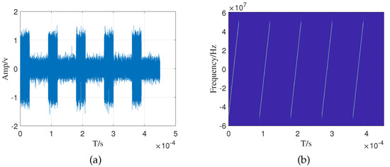
Figure 1.
The simulation results of linear frequency modulation signal. (a) Time domain waveform. (b) Time-frequency diagram.
2.2. Characterization of the RESS Model
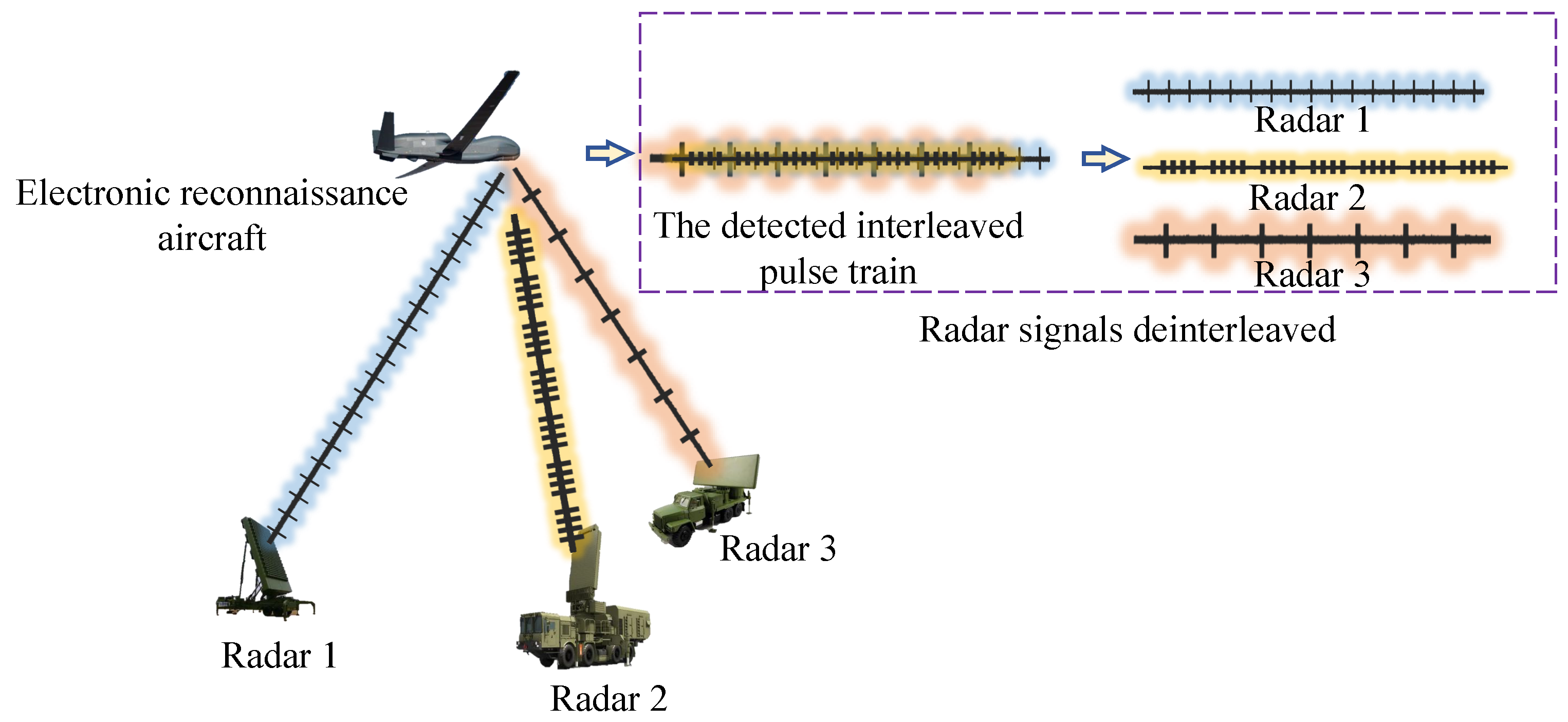
Radar reconnaissance systems generally function within intricate electromagnetic environments characterized by open spatial and frequency domains. Consequently, the data acquired by radar reconnaissance systems frequently encompass radar signals from diverse systems, varying frequency bands, and distinct signal styles. These signals interweave in the time domain, spatial domain, and frequency domain, thereby forming a complex interleaved signal flow [3]. Figure 2 depicts the process of a reconnaissance aircraft intercepting interleaved signals from three radar emitters and sorting them.
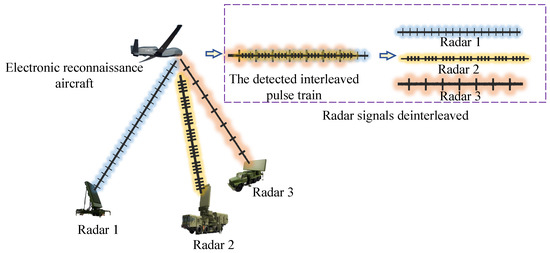
Figure 2.
The process of a radar reconnaissance aircraft intercepting and sorting signals.
To reduce radar signal sorting processing data volume and improve sorting efficiency, radar reconnaissance systems typically convert intercepted signals into interleaved PDW sequences via a measurement module. The PDW of the pulse from the radar emitter can be expressed as follows:
where represents the TOA of the pulse, represents the RF of the pulse, represents the PW of the pulse, represents the PA of the pulse, and represents the DOA of the pulse. The interleaved radar pulse sequence can be expressed as follows:
where M represents the length of the interleaved pulse sequence, and , , ( represents the number of pulses from the radar emitter and K represents the number of radar emitters), indicates that the pulse in the interleaved pulse sequence originates from the pulse of the radar emitter.
Therefore, the mathematical model of radar signal sorting can be expressed as: solving a mapping relationship that classifies the interleaved pulses according to their respective radar emitter categories. The expression is as follows:
where represents the index set corresponding to the pulses of the radar emitter in the interleaved pulse sequence. For instance, . is an indicator function used to determine whether m belongs to the set , and the corresponding expression is as follows:
2.3. Analysis of Temporal Features and Attribute Parameter Structural Relationships in Interleaved Pulse Sequences
Radar emitters usually emit pulse sequences to the target airspace in a specific timing mode (PRI modulation type) to achieve target detection [3]. Different radar emitters have particular differences in signal parameters, technical systems, and relative positions with the reconnaissance receiver. Therefore, in the interleaved pulse sequence intercepted by reconnaissance, there is a strict timing relationship between each pulse belonging to the same radar emitter, and the attribute parameter structure relationship is relatively similar.
From the perspective of pulse distribution, each pulse from the same radar emitter is strictly constrained by a certain timing mode (PRI modulation type) and runs through the sequence at all times [8]. Therefore, the temporal feature is essential in separating signals from different radar emitters. Figure 3 shows an interleaved PDW sequence diagram intercepted by the reconnaissance receiver. In this interleaved sequence, PDW1, PDW4, and PDW7 come from Radar1, and the time interval between them is ; PDW2 and PDW5 come from Radar2, and the time interval between them is ; PDW3 and PDW6 come from Radar3, and the time interval between them is .

Figure 3.
Interleaved pulse PDW time-domain distribution.
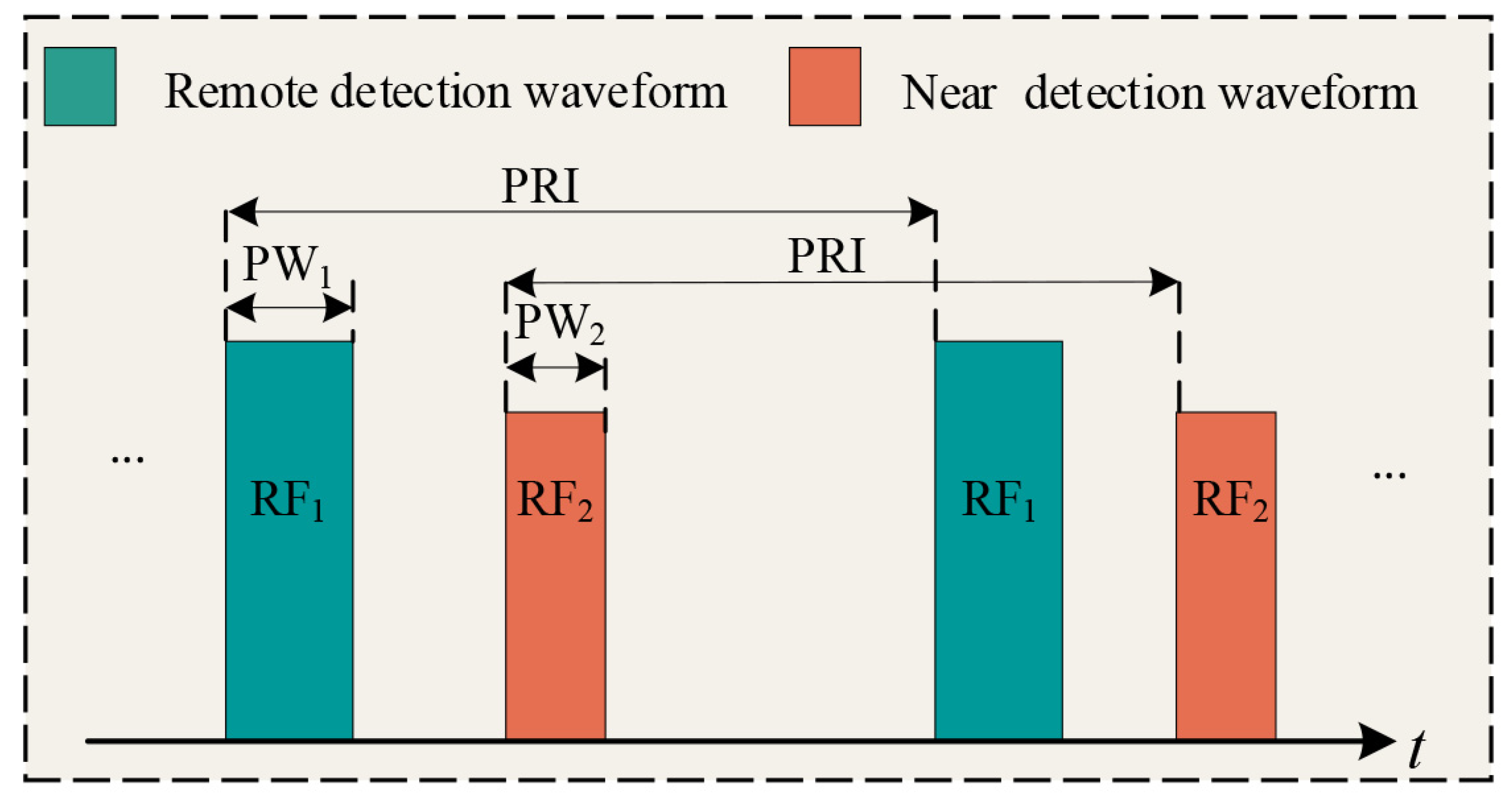
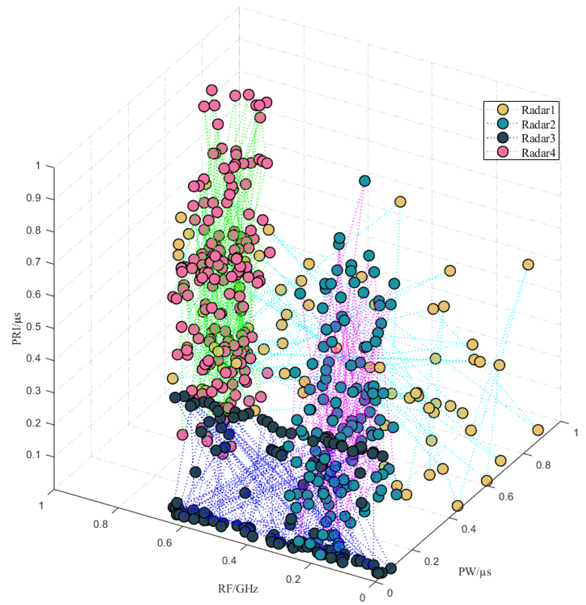
From the perspective of the structural relationship of attribute parameters, each attribute parameter from the same radar emitter is influenced by factors such as the corresponding radar system, mission, and type of target detected, and each attribute parameter’s values have inherent rules. For example, to simultaneously consider seeing targets in far and near areas, as shown in Figure 4, some radars usually alternate between emitting two signal waveforms. Typical pulse attribute parameter relationships include PRI modulation types, RF modulation types, etc. Common PRI inter-pulse relationships include fixed, jittered, sliding, staggered, dwell, etc.; common RF inter-pulse relationships include fixed, agile, diversity, step, sine, etc. Figure 5 is a structural relationship distribution diagram of attribute parameters (RF, PW, PRI) in high-dimensional space for an interleaved pulse sequence containing four radar emitters.
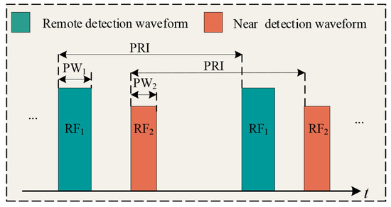
Figure 4.
Radar transmitting waveform that takes into account both far and near area detection.

Figure 5.
Visualization of pulse attribute parameters of interleaved PDW sequence.
3. Method
3.1. Overall Structure
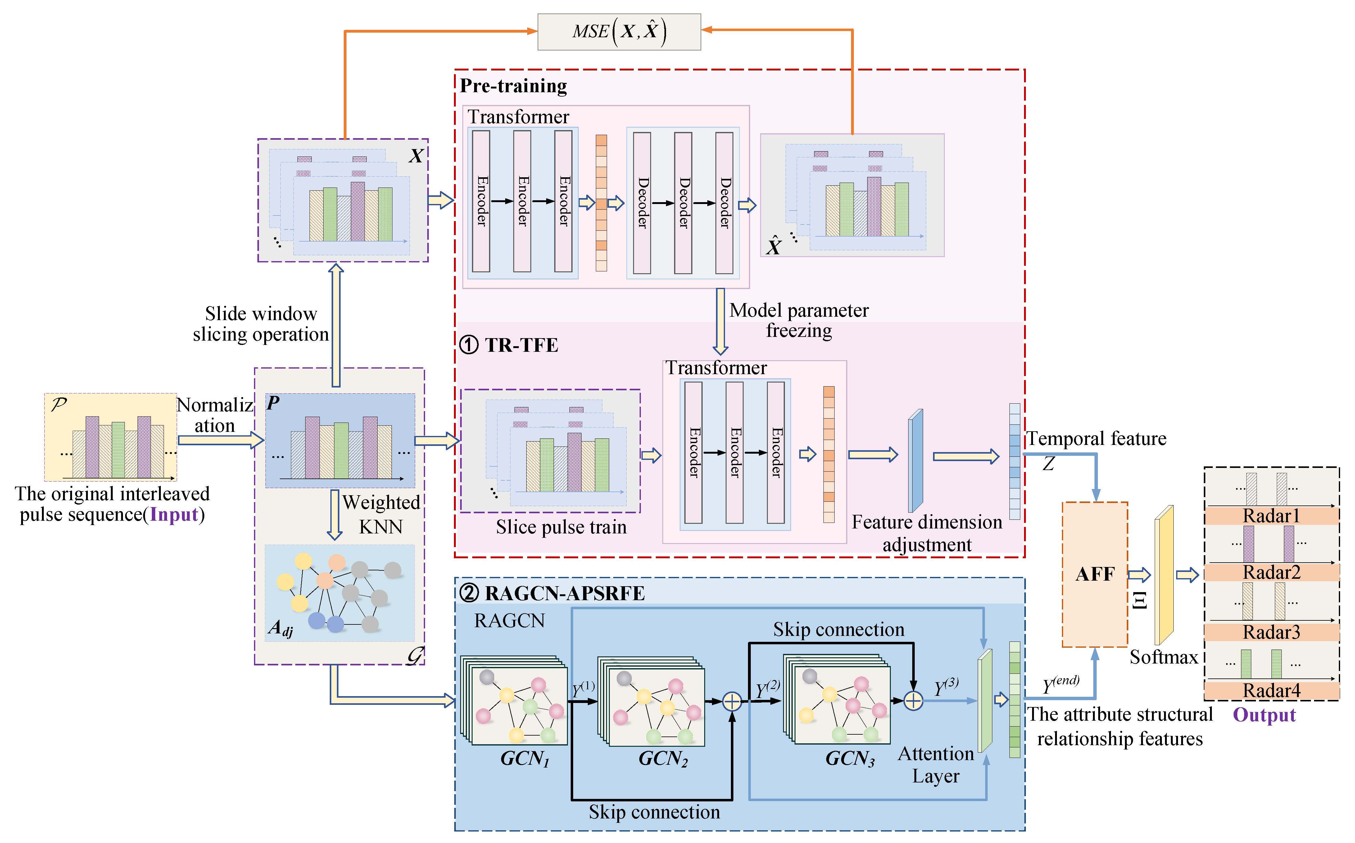
The structure of this paper’s proposed TR-RAGCN-AFF-RESS model is illustrated in Figure 6. This model primarily consists of the Transformer-based temporal feature extraction (TR-TFE) module and the RAGCN-based attribute parameter structural relationship feature extraction module (RAGCN-APSRFE). The specific process is as follows: Firstly, the original interleaved pulse sequence is normalized to obtain the pulse sequence . Using sliding window slicing and weighted KNN preprocessing methods, is preprocessed into a set of sliced pulse sequences and an undirected graph , respectively. Secondly, is input into the TR-TFE module for self-supervised pre-training. During this process, the TR-TFE network is iteratively optimized using the mean squared error loss function until it fully converges. Subsequently, the parameters of the TR-TFE network are frozen, and both and its corresponding node set are separately used as inputs to the RAGCN-APSRFE module and the TR-TFE module. The RAGCN-APSRFE module extracts pulse attribute structural relationship features from interleaved pulse sequences, while the encoder in the TR-TFE module extracts temporal features from the interleaved pulse sequences. Simultaneously, the AFF is employed to fuse the interleaved pulse sequences’ temporal features and structural relationship features. The fused features are input into the Softmax layer for pulse classification. The model is iteratively optimized using the cross-entropy loss function to achieve convergence. Finally, the test set is input into the converged model for testing, achieving precise sorting of radar emitter signals.
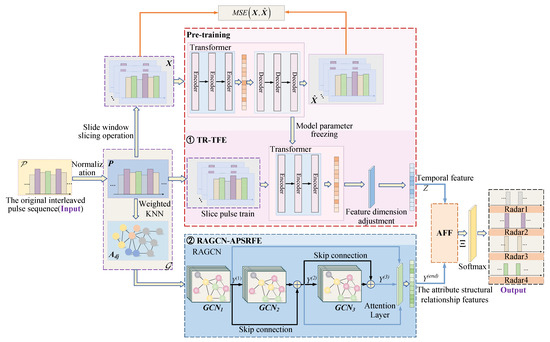
Figure 6.
The overall framework of the TR-RAGCN-AFF-RESS model.
3.2. Data Preprocessing
3.2.1. Normalization Process
The dimensions of different parameters in the PDW usually vary greatly. For instance, the unit of RF is typically GHz, while the unit of PW is usually s. Therefore, to eliminate the influence of different parameter dimensions and improve the convergence speed of the subsequent network and the sorting accuracy, it is necessary to normalize each parameter in the interleaved pulse sequence according to the expression as follows:
where x represents the parameter vector that needs to be normalized.
3.2.2. Generation of Graph Data for the Interleaved Pulse Sequence
In order to characterize the structural relationships of pulse attribute information in the interleaved pulse sequence, this paper represents the interleaved pulse sequence as an undirected graph. Specifically, in the interleaved radar emitter pulse sequence , each pulse is considered a node, with the PDW parameters of each pulse serving as the node’s attributes. Therefore, an undirected graph of an interleaved pulse sequence can be represented as , where represents the node set, and represents the edge set. is usually represented by an adjacency matrix . For any two nodes and in the undirected graph, where , . If there is a mutual connection between them, then , otherwise , and it holds that . Therefore, computation of the adjacency matrix is the key to generating graph structure data for the interleaved pulse sequence.
Traditionally, when constructing an adjacency matrix, it is assumed that the connection weights between all nodes are the same. However, in the task of RESS, there will be errors in the attribute parameters of each node due to the presence of measurement errors. When attribute information with significant errors propagates and aggregates in the neural network, it will severely affect the sorting effect of RESS. In order to increase the proportion of attribute information closely related to the current radar emitter emission signal, effectively propagating and aggregating in the neural network, and at the same time suppress the adverse effects brought by attribute information with significant measurement errors, this paper proposes a method for generating a weighted adjacency matrix. The process is as follows: Firstly, the k-nearest neighbor (KNN) algorithm is used to calculate the K most adjacent samples for each pulse in the interleaved pulse sequence, and the initial adjacency matrix is constructed based on the calculation results. Secondly, the Euclidean distance is used to measure the approximate relationship between the current pulse in the high-dimensional parameter space and its corresponding K-nearest neighbor pulses. Suppose the K nearest samples corresponding to the pulse are . The Euclidean distance from the pulse to any of its nearest samples is defined as follows:
where represents the parameter of the nearest pulse, L represents the number of attribute parameters in the pulse, and represents the parameter of the pulse . Thirdly, we use weights to characterize the importance of the approximate relationship between the current pulse and its corresponding K-nearest neighbor pulses. The expression for this weight is as follows:
Finally, a weight matrix is introduced to correct the initial adjacency matrix . The expression for the weight matrix is as follows:
where the subscript k represents the index of pulse in the k-nearest samples of pulse . Then, the expression for the corrected weighted adjacency matrix is as follows:
where ⊙ represents the Hadamard product of matrices.
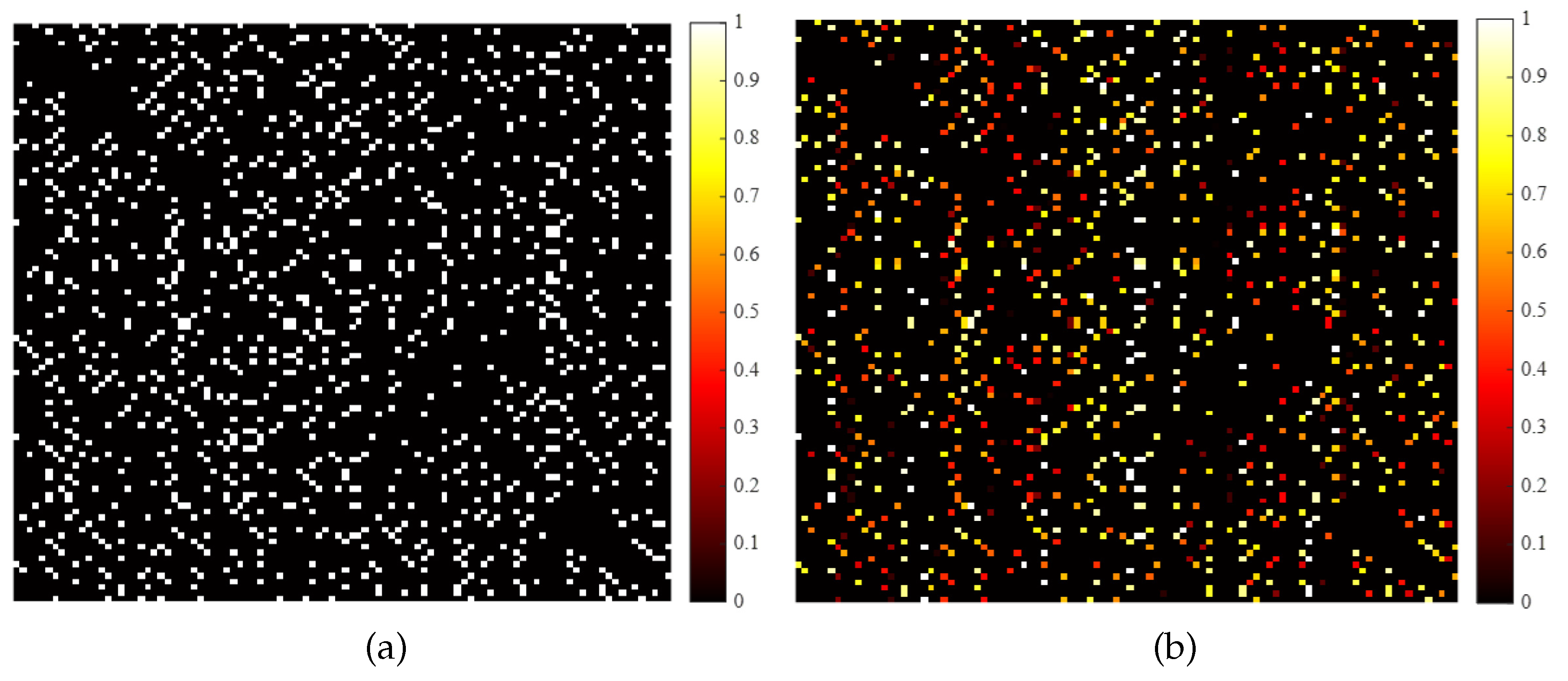
Figure 7a,b represent the unweighted and weighted adjacency matrices corresponding to 100 interleaved pulses. In the unweighted adjacency matrix, the connection weights between neighboring node pulses with a connection relationship are the same. Therefore, its visualization of the adjacency matrix only contains two types of relationships, black and white, where black indicates no connection relationship and white indicates that two pulses have a connection relationship with a weight of 1. The connection relationships between neighboring node pulses are allocated according to certain weights in the weighted adjacency matrix. Therefore, its corresponding visualization contains multiple colors, allowing pulses with close connection relationships to play a more significant role in the sorting task.
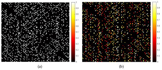
Figure 7.
Visualization results of adjacency matrix. (a) Unweighted adjacency matrix. (b) Weighted adjacency matrix.
3.3. Temporal Feature Extraction Based on Transformer
In order to effectively extract the temporal features of the interleaved pulse sequence in scenarios with a limited number of labeled samples, this paper uses a complete Transformer as the feature extraction network and constructs an encoder–decoder structure for the feature extractor.
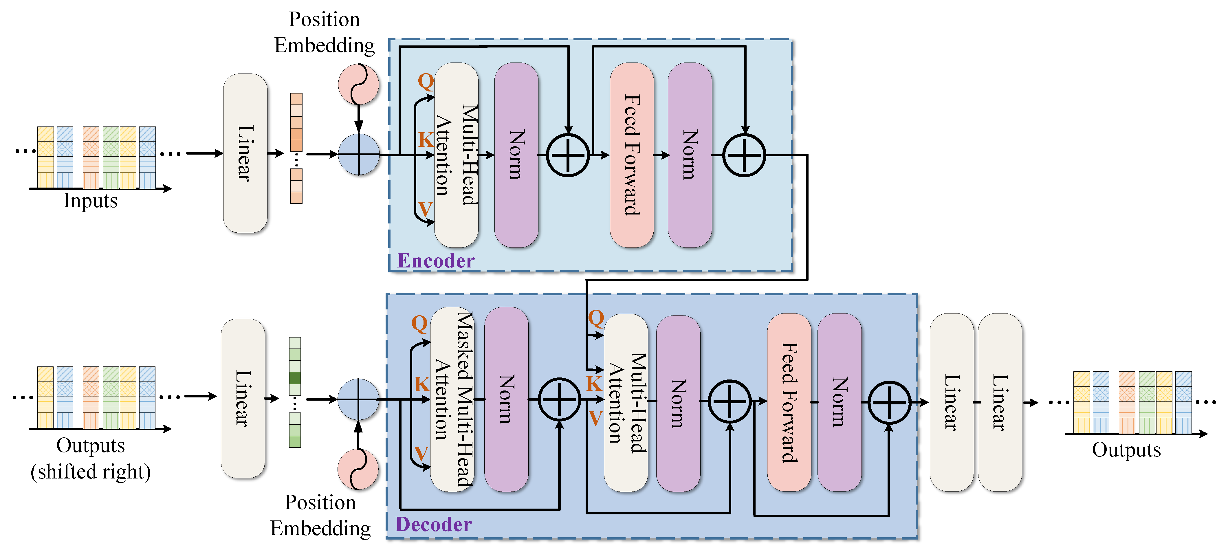
Transformer [33] is an exceptional network for temporal feature extraction [34,35]. Figure 8 illustrates the complete structure of the Transformer, which is composed of two elements: the encoder and the decoder. The encoder’s role is to map the input data into a feature space, while the decoder utilizes these features to reconstruct the original sequence. The encoder and decoder comprise modules like multi-head attention mechanisms, feed-forward neural networks, and residual connections. The multi-head attention mechanism is responsible for extracting parallel features from the input data, while the positional encoding mechanism records the data’s positional information, thereby ensuring feature correlation.
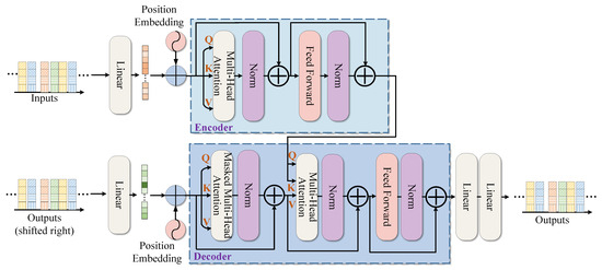
Figure 8.
The complete structure of the Transformer.
- (1)
- Positional Encoding
Radar pulse sequences exhibit strict temporal relationships. However, since the Transformer does not extract features from input data sequentially, it cannot effectively utilize the temporal relationships within sequence data. To fully leverage the temporal information in pulse sequences, position encoding is commonly employed in Transformers to record the positional information of pulse sequence data. For an input pulse sequence , the position encoding formula [33] can be expressed as follows:
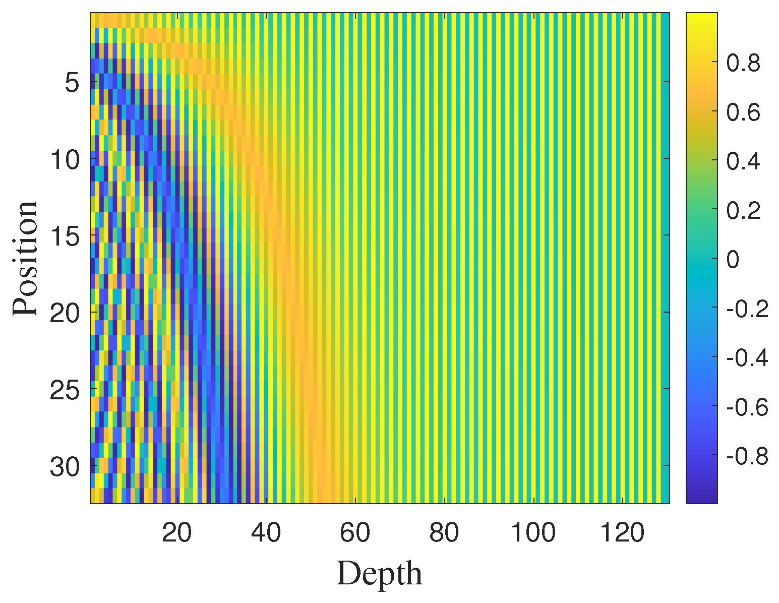
where represents the position encoding, represents the actual position of the current pulse in the input pulse sequence, is the dimension of the position encoding, and and , respectively, represent even and odd positions. The adoption of the above form of position encoding formula implies that each dimension of the position encoding corresponds to a sine wave, which can make be represented as a linear function of for any fixed offset k, thereby making it easier for the neural network to learn the position information [33]. For instance, for a pulse sequence containing 32 pulses, an embedding is learned using a fully connected layer. The corresponding position encoding results are depicted in Figure 9.

Figure 9.
Position encoding results for the pulse sequence .
- (2)
- Multi-Head Attention Mechanism
The self-attention mechanism is the core structure of the Transformer. Its principle is as follows: Firstly, three types of linear transformations are performed on the input data to obtain the (Query), (Key), and (Value) matrices. Then, the dot product of and is calculated to obtain the weight matrix . The weight matrix is divided by a scaling factor to prevent the inner product from becoming too large. Finally, the Softmax function is used to normalize the results, which are then multiplied by to obtain the final result. The mathematical expression of the self-attention mechanism is as follows:
The multi-head attention mechanism is composed of multiple self-attention mechanisms in parallel. For a multi-head attention mechanism with n heads, its expression can be expressed as follows:
where represents the attention head, and , , , and represent the parameter matrices [33]. Using a multi-head attention mechanism facilitates the thorough integration of information from various attention heads, consequently enhancing the feature representation of the initial data.
The process of temporal feature extraction based on Transformer can be described as follows: Let represent the encoder in the Transformer, and represent the decoder. For the input interleaved pulse sequence , the encoding and decoding process can be expressed as follows:
where Z represents the hidden features output by the encoder, represents the weight coefficients of the neural network, represents the bias coefficients of the neural network, represents the input sample space, represents the feature space, and represents the pulse samples generated by the decoder. The key to extracting effective temporal features with an encoder–decoder structure is minimizing the difference between the input and regenerated samples. Since both the input and output of the model are normalized pulse sequences, the mean square error function is chosen as the optimization objective function, which is expressed as follows:
where represents the mean squared error function, represents the normalized pulse input, and represents the recovered normalized pulse. By iterative training and minimizing the minimum mean square error between the input and output, a network that accurately extracts the temporal features of the interleaved pulse sequence can be obtained.
3.4. Pulse Attribute Parameter Structural Relationship Feature Extraction Based on RAGCN
Once the interleaved radar pulse sequence is converted to graph-structured data, the problem of deinterleaving the pulse sequence can be transformed into a node classification problem. The corresponding mathematical model can be expressed as follows:
where represents the graph neural network model, and represents the classification result. In order to better achieve the above goals, we propose the RAGCN model, mainly composed of graph convolutional layers, residual connections, and layer attention.
Graph convolutional layers can aggregate the features of neighboring nodes based on the given graph structure to obtain the feature representation of the node. This process mainly includes three steps: aggregation, update, and loop iteration. For the graph , its corresponding weighted adjacency matrix is , and the propagation process of the layer graph convolution layer can be expressed as follows:
where represents the activation function, represents the feature representation of the current node in the layer, is the degree matrix of the current node and is a diagonal matrix, represents the weight of the layer, , and I is a unit matrix. Although graph convolutional layers can learn the feature representation of node data well, there is also the problem of over-smoothing. In order to avoid this problem, skip connections are created between layers 1 and 2 and between layers 2 and 3. This allows layers 2 and 3 to engage in residual learning behavior, which accelerates convergence speed and alleviates the problem of over-smoothing caused by the network being too deep. In addition, to improve the feature representation of nodes in graph convolutional neural networks, a layer attention mechanism is introduced to embed the outputs of different graph convolutional layers into the final feature expression according to specific weight coefficients. The expression for the weight coefficient of the layer output feature in the final feature expression is shown in Equation (22).
By embedding the output features of each graph convolution layer into the final feature expression according to a certain weight, the attribute parameter structural relationship features extracted by RAGCN can be finally expressed in the following form:
where U represents the number of layers in the graph convolutional layer, represents the attribute parameter structural relationship features extracted by RAGCN, and represents the output features of the layer in RAGCN.
Finally, the attribute parameter structural relationship features extracted by RAGCN and the temporal features extracted by Transformer are fused using the AFF method. The fused features are then input into the classification layer to achieve the sorting of radar emitter signals.
3.5. AFF
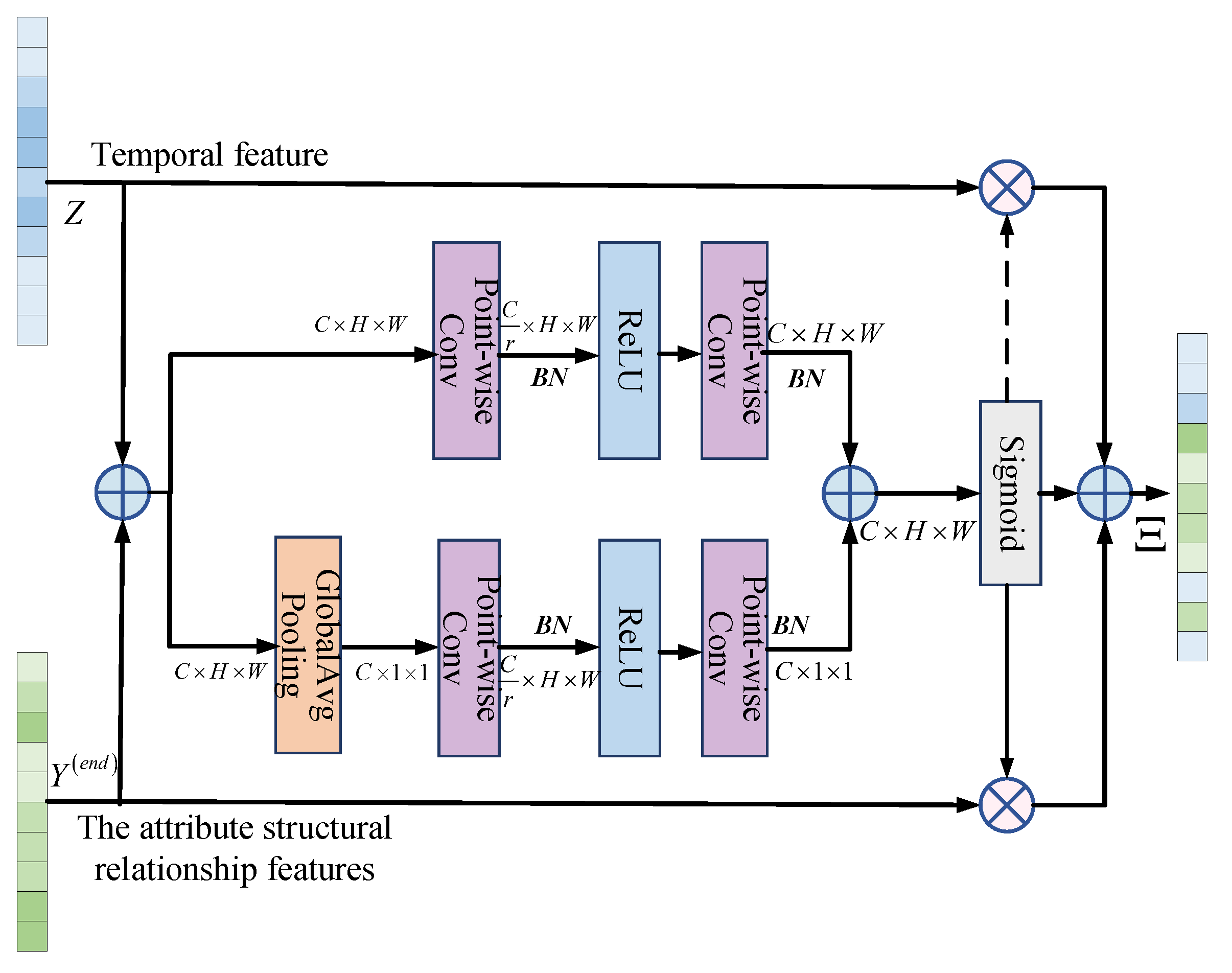
AFF is mainly used to fuse features of different scales from different networks, and it is a plug-and-play method for multi-feature fusion [36]. In this paper, AFF is used to fuse the temporal features Z extracted from Transformer and the attribute parameter structural relationship features from RAGCN. The structure diagram of AFF is shown in Figure 10.
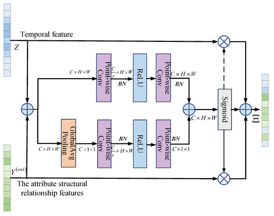
Figure 10.
AFF structure diagram.
The specific process of AFF is as follows: Firstly, add and merge the input temporal features Z and the attribute parameter structural relationship features . Secondly, the result after addition is divided into two branches: global attention and local attention extraction. Thirdly, the extracted global and local features are added again. Finally, the weights of Z and are calculated separately through the Sigmoid function, and the weighted average feature is obtained. By inputting the fused feature into the Softmax classifier and predicting according to Equation (24), the final node classification result can be obtained.
To endow the feature extractor with good feature mining performance, optimizing the model by incorporating the predicted classification error into the cost function is necessary. As this paper converts the task of sorting radar emitter signals into a multi-classification task of graph data nodes, the cross-entropy loss function is chosen as the cost function to measure the accuracy of the model’s predicted classification results. The expression for the cost function is shown in Equation (25).
4. Experiment
4.1. Setting
4.1.1. Dataset
Because the parameters of radar emitter signals are military secrets of various countries, it is not easy to obtain the corresponding datasets. In order to verify the effectiveness of the algorithm’s effectiveness proposed in this paper, we test the algorithm using a simulated dataset. This paper simulates the PDW data of four radar emitters based on the parameter settings in reference [10], where each radar has 1 to 3 working modes. Table 1 shows the detailed simulation parameter settings, where the ‘number’ represents the number of pulses emitted by each radar emitter in the corresponding working mode. In the simulated interleaved pulse sequence, each pulse signal is characterized by a PDW, which includes five parameters: DOA, PW, RF, PRI, and TOA.

Table 1.
Simulation parameter settings.
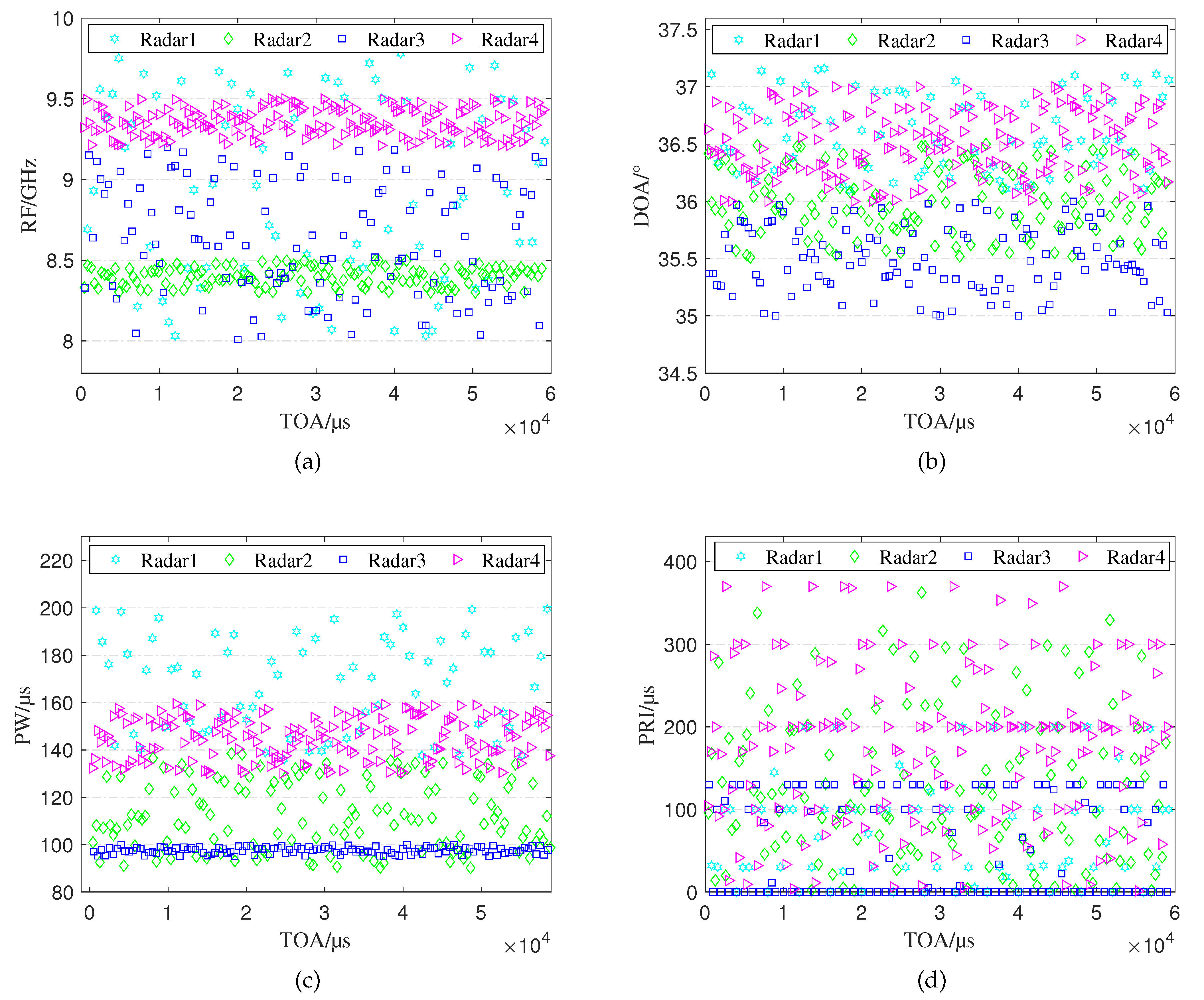
The distribution of the interleaved pulse PDW train of the four radar emitters is shown in Figure 11, where Figure 11a is the distribution of RF, Figure 11b is the DOA distribution, Figure 11c is the PW distribution, and Figure 11d is the PRI distribution. To simulate the intercepted interleaved pulse trains as realistically as possible, we set the parameter value range and the pulse interval modulation type of different radar emitters to have a certain degree of overlap. The simulation dataset will eventually be divided into a training set, a validation set, and a test set according to a certain ratio.
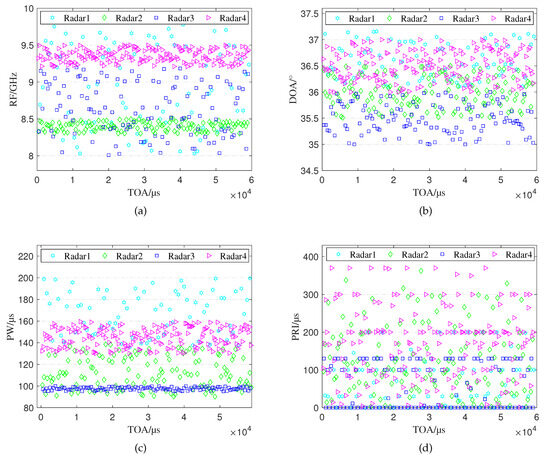
Figure 11.
The distribution of simulation data. (a) The distribution of RF. (b) The distribution of DOA. (c) The distribution of PW. (d) The distribution of PRI.
4.1.2. Simulation Settings
The experiments in this paper were conducted on a high-performance desktop workstation equipped with the Windows 11 operating system and an RTX 3090 GPU from NVIDIA Corporation in Santa Clara, CA, USA. The network structure was built in the integrated development environment PyCharm 2019.3, with the necessary environment, including PyTorch 1.120 and Python 3.8.13. The parameter settings for pre-training the Transformer network are shown in Table 2, and the parameters for training RAGCN are shown in Table 3.

Table 2.
Parameter settings of Transformer.

Table 3.
Parameter settings of RAGCN.
Due to the limitations of radar signal reconnaissance conditions in actual electronic warfare, the pulse sequence that the reconnaissance receives will typically contain a certain percentage of measurement errors, lost pulses, and spurious pulses, among other non-ideal situations. To test the deinterleaving performance of the proposed algorithm under the aforementioned non-ideal conditions, we have constructed experimental scenarios that include different measurement errors, lost pulse ratios, and spurious pulse ratios. The parameter settings are shown in Table 4. Specifically, the measurement error of a pulse is simulated by adding Gaussian noise with a mean of zero and a variance of to the pulse train [37]. The spurious pulse is simulated by randomly inserting random pulse into the original interleaved pulse train [37]. The lost pulse condition is simulated by randomly deleting of the pulses in the original interleaved pulse train [37].

Table 4.
Parameter settings for different experimental scenarios.
4.1.3. Baseline Methods
To further evaluate the effectiveness of the proposed method, this paper selects several representative radar signal sorting methods for comparison. The descriptions of each method are as follows:
- (1)
- ResGCN [10]: This method adopts a semi-supervised learning approach, transforming the problem of deinterleaving radar emitter signals into a graph data node classification problem, providing a new perspective for RESS.
- (2)
- Bi-LSTM [38]: This method adopts two long-term memory network structures, forward and backward, which can better learn the sequential dependence of sequence data and obtain a better classification effect.
- (3)
- TCN [39]: The core of this method consists of dilated causal convolution and residual modules, which can simultaneously combine the advantages of convolutional neural networks and recurrent neural networks, effectively overcoming the problems of high memory usage and poor parallelism during the training of recurrent neural networks. It has been widely used in the processing of radar pulse sequences [8,40].
- (4)
- GRU [41]: This network is a variant of LSTM, with fewer parameters and a more straightforward network structure than LSTM. Moreover, it can perform similarly to LSTM in processing time series data.
- (5)
- PSO-K [42]: This method is an unsupervised approach that effectively combines the particle swarm optimization algorithm, which has excellent global optimization capabilities, with the k-means clustering method. It can effectively overcome the problem of the k-means algorithm quickly falling into local optima, significantly improving the clustering effect.
- (6)
- DBSCAN [43]: This method is also a classic unsupervised density clustering algorithm that has been used to solve the problem of RESS. However, this method suffers from the issue of clustering parameter settings that heavily rely on expert experience, which often leads to unsatisfactory clustering results.
4.1.4. Evaluation Metrics
In order to quantitatively evaluate the performance of the algorithm proposed in this paper in the task of RESS, the following evaluation metrics are used to describe the results quantitatively:
- (1)
- Mean Accuracy: The mean accuracy measures the proportion of correctly sorted pulses in the total number of pulses in the test set. Suppose the number of pulses in the test set is ; then, the mean accuracy can be expressed as follows:where represents the number of radar emitter, c represents the label corresponding to the current radar emitter, and [8] represents the true positive prediction results of the radar emitter with label c.
- (2)
- Precision: Precision reflects the proportion of true positive samples in the predicted positive results. The expression for the prediction precision of the radar emitter is as follows:where [8] represents the false positives of the corresponding category. The mean precision of the radar emitter sorting results can be expressed as follows:
- (3)
- Recall: Recall describes the proportion of samples predicted as positive in the actual positive samples. The recall of the radar emitter with label c is defined as follows:where [8] represents the false negatives of this category. The mean recall of RESS results can be expressed as follows:
4.2. Experimental Results and Analysis
4.2.1. Comparative Experiment
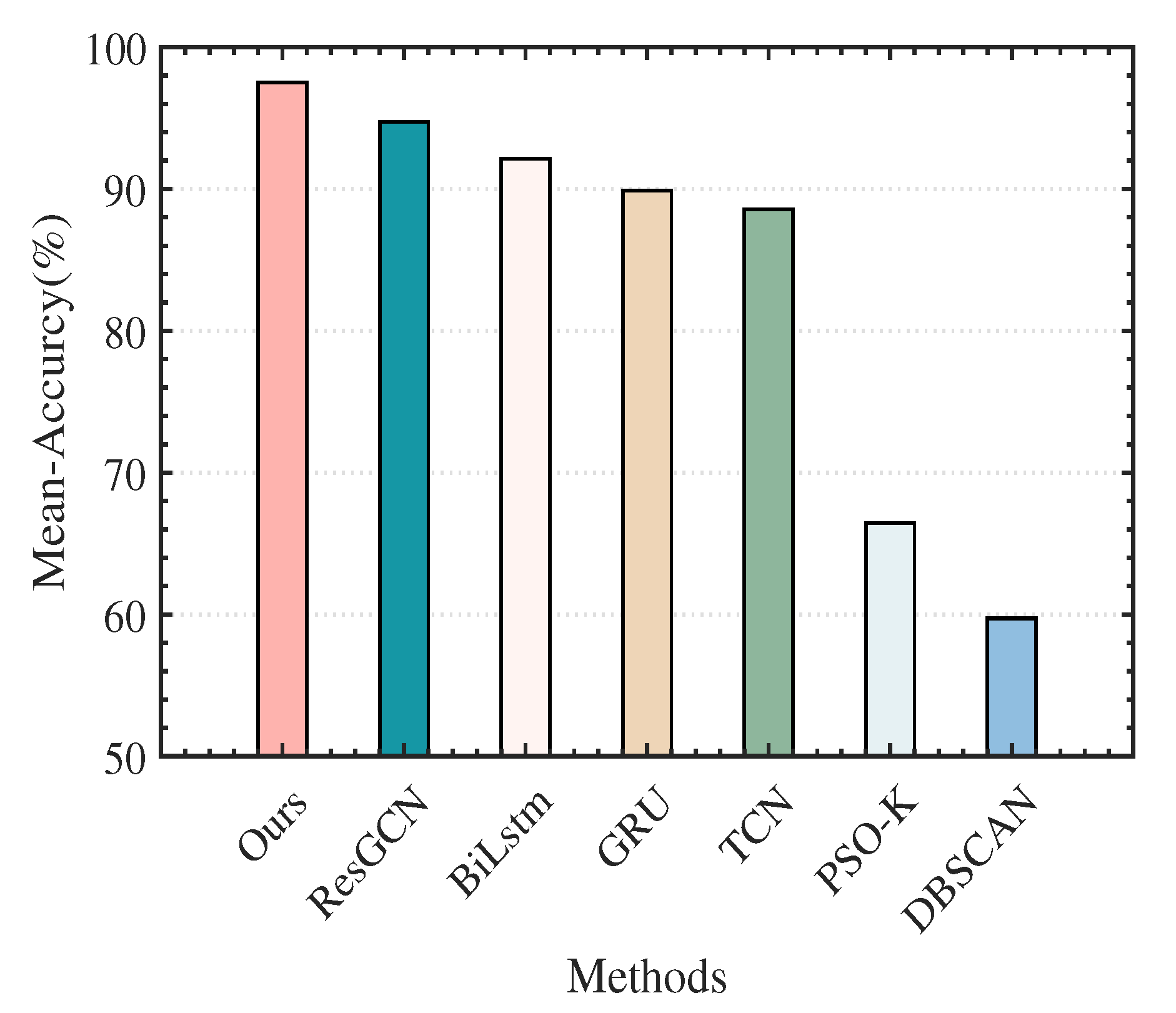
The validity of our method was tested by using 10% of the pulses without measurement errors, lost pulses, and spurious pulses as the training set; 45% of pulses as the verification set; and another 45% of pulses as the testing set. The sorting precision, recall rate, and mean accuracy of different algorithms are shown in Table 5 and Table 6, and Figure 12.

Table 5.
Precision of different RESS methods.

Table 6.
Recall of different RESS methods.
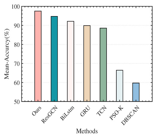
Figure 12.
Mean accuracy of different RESS methods.
The results of the experiments show that our method not only realized excellent sorting precision and recall rates on Radar 1, Radar 2, Radar 3, and Radar 4 but also achieved the highest mean accuracy on the total sorting results, exceeding those of any other baseline methods. This because the proposed method fully integrates the temporal and attribute parameter structural relationship features of the interleaved pulse sequence, enriches the feature expression of the original pulse, and improves the separability of the pulse. In contrast, the sorting results of ResGCN, Bi-LSTM, GRU, TCN, PSO-K, and DBSCAN are relatively poor. The underlying reason for this is that these methods can only extract a single feature (temporal or attribute parameter structural relationship feature) from the radar pulse sequence. Specifically, the ResGCN algorithm transforms the task of RESS into a graph structure data node classification problem, only utilizing the attribute parameter structural relationship features of the interleaved pulse sequence. Bi-LSTM, GRU, and TCN are all methods for handling time series data. In particular, because Bi-LSTM uses both forward and backward LSTM structures, it extracts richer temporal features; thus, its sorting results are better than those of TCN and GRU. However, when the number of training samples is small, the sorting results are greatly affected. The PSO-K algorithm and the DBSCAN algorithm use the similarity between pulse parameters and the local density of data to sort the radar emitter signals, respectively. The sorting effect is unsuitable for this interleaved pulse situation with severe parameter attribute overlap.
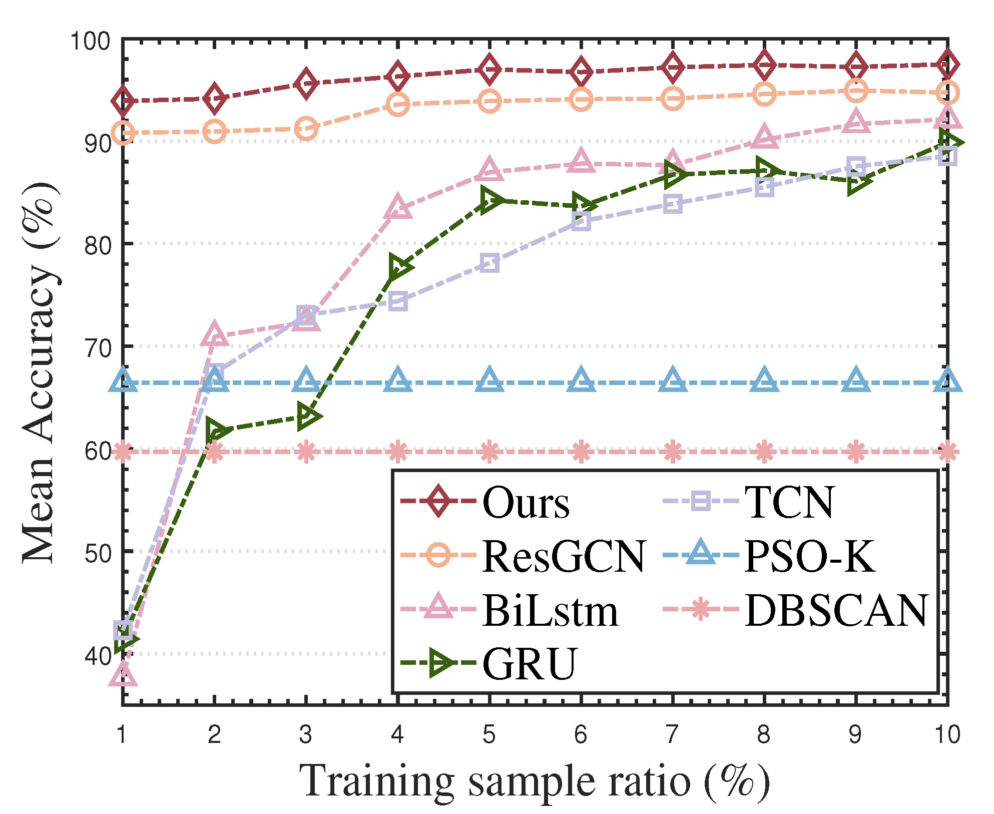
In order to further test the effectiveness of our proposed algorithm at different levels of labeled sample quantities, we set the number of training samples in different proportions under the completely ideal interleaved pulse sequence. We obtained the sorting results in Figure 13. As the number of training samples gradually decreases, the mean accuracy of sorting by all methods has different degrees of decline. However, the decline speed of our method is the slowest, and the mean sorting accuracy in all cases is better than 93.91%. The above results prove that the sorting effect of our proposed algorithm under the scenario of limited labeled sample quantity is better than the existing supervised sorting methods and unsupervised clustering methods.
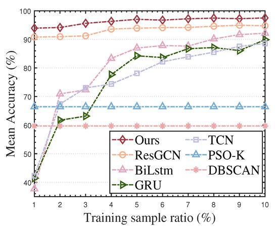
Figure 13.
Mean accuracy of various RESS algorithms under different proportions of training samples.
4.2.2. Robustness Experiment
In the actual received radar interleaved pulse sequence, there will inevitably be non-ideal situations such as a certain degree of measurement error, lost pulses, and spurious pulses. In order to test the robustness of the proposed method in this paper, we tested the algorithm in various scenarios: only measurement errors, lost pulses, spurious pulses, and a complex scenario that includes all three non-ideal conditions. In each experimental scenario, 10% of the samples were selected as the training set, 45% of the samples were selected as the validation set, and 45% of samples were selected as the test set.
- (1)
- Situation with Only Measurement Error
By adding different levels of measurement error to the ideal radar interleaved pulse sequence (as shown in Table 4), we test the sensitivity of the method proposed in this paper to measurement error. Figure 14a–c shows the experimental results under different levels of measurement error. As the measurement error situation worsens, the mean accuracy of RESS shows a certain downward trend. The reason for this may be that the measurement error causes further overlap of the parameter attributes of the radar emitter, and the attribute parameter structural relationship features or temporal features of the signal belonging to the same radar emitter are damaged to a certain extent. However, the mean accuracy of the sorting method proposed in this paper does not drop rapidly with the increase in the measurement error level; the overall fluctuation range is less than 2%, and even in the case of the highest level of measurement error, it can still achieve a mean correct sorting rate of 89.75%. The result indicates that the TR-RAGCN-AFF model has good robustness to measurement errors.

Figure 14.
The result of RESS under different levels of measurement error. (a) Precision. (b) Recall. (c) Mean Accuracy.
- (2)
- Situation with Only Lost Pulses
In practice, the high pulse flow density of the environment can easily cause lost pulses. To test the sorting ability of our method at different lost pulse levels, we construct this environment by deleting a certain proportion (as shown in Table 4) of the original pulses in the ideal radar interleaved pulse sequence. Figure 15a–c shows the sorting results of each radar emitter signal under different lost pulse levels. As the proportion of lost pulses increases from 10% to 50%, the sorting effect continues to decline. The potential reason may be that, on the one hand, as the proportion of lost pulses continues to increase, the number of training samples further decreases, and it is difficult for the feature extractor to learn effective features; on the other hand, the lost pulses destroy the temporal regularity of the original pulse sequence. However, the fluctuation ratio of the mean sorting accuracy of our algorithm in all cases is less than 4%, and even when the lost pulse ratio reaches 50%, it can still achieve an average sorting accuracy of 88.19%. The result shows that the method we proposed has good applicability to the situation of lost pulses.

Figure 15.
The result of RESS under different proportions of lost pulses. (a) Precision. (b) Recall. (c) Mean Accuracy.
- (3)
- Situation with Only Spurious Pulses
Due to pulse splitting and pulse overlapping, there is a certain proportion of spurious pulses in the received pulse train. We simulate different levels of spurious pulse situations by randomly replacing 10% to 50% of the pulses in the ideal interleaved pulse sequence. Figure 16a–c shows the sorting results under different proportions of spurious pulses. As the proportion of spurious pulses increases from 10% to 50%, the sorting results significantly decline. The reason may be that with the augmentation of the spurious pulses, the temporal relationship and attribute parameter structural relationship features of pulses from the same radar emitter become badly damaged, which makes it hard for the sorting algorithm to obtain useful differential features. However, because the method proposed in this paper simultaneously integrates the different features of the pulse sequence, the feature information is complemented to a certain extent. Therefore, when the proportion of spurious pulses is less than or equal to 40%, the mean sorting accuracy is better than 62%, indicating that our algorithm still has good applicability under extreme spurious pulse conditions.

Figure 16.
The result of RESS under different proportions of spurious pulses. (a) Precision. (b) Recall. (c) Mean Accuracy.
- (4)
- Complex Situation with Measurement Error, Lost Pulses, and Spurious Pulses Simultaneously
In the intercepted radar pulse sequence, non-ideal situations such as measurement errors, lost pulses, and spurious pulses often exist simultaneously. This section aimed to test the algorithm proposed in this paper in complex situations. We construct five complex non-ideal scenarios that simultaneously contain measurement errors, lost pulses, and spurious pulses at different levels (as shown in Table 4). The sorting results are shown in Figure 17a–c. As the complexity of the scenario continues to increase, the performance of all algorithms has declined to a certain extent. However, the mean accuracy, precision, and recall of the algorithm we proposed have reached their best in various complex scenarios. Despite the time-domain measurement error being at most 2 s, the frequency-domain measurement error is no more than 2 MHz, the angle measurement error not exceeding , and the combined proportion of lost and spurious pulses being up to 40%, the mean accuracy, precision, and recall values remain above 60%. The result above indicates that the method proposed in this paper has good applicability in complex electromagnetic environments, which is of obvious significance for the practical application of this method.

Figure 17.
The result of different RESS methods in complex scenarios. (a) Mean accuracy. (b) Mean precision. (c) Mean recall.
4.2.3. Ablation Experiment
In order to verify the effectiveness of the sub-modules, such as the weighted adjacency matrix, residual attention, and temporal feature fusion in TR-RAGCN-AFF, we conducted experiments using the ideal radar interleaved pulse sequence as samples. We used 10% of the samples as the training set, 45% of the samples as the validation set, and another 45% of the samples as the test set and tested the effectiveness of each module under four different scenarios.
Table 7 presents the experimental results for four scenarios, where “✔” denotes the inclusion of a sub-module in the current experiment, and “×” signifies its removal. The mean sorting accuracy, precision, and recall rate of scenario 2 improved by 0.27%, 0.53%, and 0.93%, respectively, compared to scenario 1. The reason is that the weighted adjacency matrix in scenario 2 can enhance the aggregation of pulses belonging to the same class in the graph structure data, enabling the GCN to extract more distinct structural features. The mean sorting accuracy, precision, and recall rate of scenario 3 improved by 1.58%, 1.51%, and 2.58%, respectively, compared to scenario 1. The fundamental reason for this is that scenario 3 not only adds a weighted adjacency matrix but also introduces a residual attention structure in the GCN. By embedding the features extracted from different graph convolution layers into the final feature layer using residual attention, the feature representation of the interleaved radar pulse sequence can be enriched to a certain extent, thereby improving the node classification accuracy. Compared to scenario 1, the mean sorting accuracy, precision, and recall rate of scenario 4 improved by 2.76%, 2.64%, and 4.47%, respectively. This indicates that the integration of temporal features plays a significant role in the sorting effect of radar emitter signals. In converting the interleaved pulse sequence into graph structure data, the temporal features in the pulse sequence will be lost, which is disadvantageous when the number of training samples is small. However, by adopting AFF to integrate some temporal features based on extracting attribute parameter structural relationship features, it is possible to achieve complementary features in different domains, thereby raising the upper limit of accuracy. When not using modules such as the weighted adjacency matrix, residual attention, and temporal feature fusion, instead adopting ResGCN [10], as shown in scenario 1, the mean sorting accuracy, precision, and recall rate are all at their worst. This is because, compared to the ResGCN algorithm, our algorithm, on the one hand, introduces an attention residual structure when extracting attribute parameter structural relationship features from the interleaved pulse sequence, effectively enriching the final feature expression and proposes a data preprocessing method for the weighted adjacency matrix and allowing attribute parameters closely related to the radar emitter signal features to be more effectively propagated and aggregated in the neural network. On the other hand, we consider the temporal features in the interleaved pulse sequence and construct an encoder–decoder structure for the temporal feature extractor. In addition, the AFF algorithm is introduced to fuse features from different domains (temporal features and attribute parameter structural relationship features) fully, promoting complementarity between features and reducing feature redundancy. The results and analysis confirm that the sub-modules (weighted adjacency matrix, residual attention, temporal feature fusion) introduced in our proposed method all have tangible performance improvements for RESS.

Table 7.
Ablation experiment results.
5. Conclusions
This paper proposes a method for RESS that integrates temporal features and pulse attribute parameter structural relationship features. We propose a method for constructing a weighted adjacency matrix, which improves the accuracy of describing the attribute parameter structural relationship in the interleaved pulse sequence. On this basis, an attribute parameter structural relationship feature extraction network based on RAGCN and a temporal feature extraction network based on Transformer are constructed, respectively. Finally, the AFF algorithm is introduced to fully fuse features from different domains, effectively raising the upper limit of the sorting accuracy of RESS. Simulation results under various non-ideal conditions show that, compared with existing methods, our method has higher mean sorting accuracy, precision, recall rate, and robustness in complex electromagnetic environments with limited labeled sample numbers. This is of significant practical importance for cognitive electronic warfare systems for precision jamming. It is worth noting that the objects of radar reconnaissance may be completely unknown targets, leading the emitter source signal sorting task to face zero-sample situations. Our model currently struggles to cope with the above situation. Solving the radar emitter signal sorting problem in the absence of prior information is the focus of our future research.
Author Contributions
Conceptualization, Z.Z.; methodology, Z.Z. and X.G.; validation, Z.Z.; investigation, X.S. and X.G.; resources, Z.Z.; data curation, X.G.; writing—original draft, Z.Z.; writing—review and editing, Z.Z. and X.S.; Funding acquisition, F.Z. All authors have read and agreed to the published version of the manuscript.
Funding
This work was supported in part by the National Natural Science Foundation of China under Grant 61201418 and Grant 62101412; in part by the Postdoctoral Science Research Projects of Shaanxi Province under Grant 2018BSHEDZZ39; and in part by the Fundamental Research Funds for the Central Universities under Grant ZDRC2207 and ZYTS23146.
Data Availability Statement
Data sharing is not applicable to this article.
Conflicts of Interest
The authors declare no conflicts of interest.
References
- Feng, H.; Tang, B.; Wan, T. Radar pulse repetition interval modulation recognition with combined net and domain-adaptive few-shot learning. Digit. Signal Process. 2022, 127, 103562–103573. [Google Scholar] [CrossRef]
- Chi, K.; Shen, J.; Li, Y.; Wang, S. Multi-Function Radar Signal Sorting Based on Complex Network. IEEE Signal Process. Lett. 2021, 28, 91–95. [Google Scholar] [CrossRef]
- Liu, Z. Intelligent Processing of Radar Singals in Reconnaissance System; National Defense Industry Press: Beijing, China, 2023; pp. 9–120. [Google Scholar]
- Zhu, M.; Wang, S.; Li, Y. Model-Based Representation and Deinterleaving of Mixed Radar Pulse Sequences with Neural Machine Translation Network. IEEE Trans. Aerosp. Electron. Syst. 2022, 58, 1733–1752. [Google Scholar] [CrossRef]
- Li, X.; Liu, Z.; Huang, Z. Deinterleaving of Pulse Streams with Denoising Autoencoders. IEEE Trans. Aerosp. Electron. Syst. 2020, 56, 4767–4778. [Google Scholar] [CrossRef]
- Liu, Y.; Zhang, Q. Improved Method for Deinterleaving Radar Signals and Estimating PRI Values. IET Radar Sonar Navig. 2018, 12, 506–514. [Google Scholar] [CrossRef]
- Liu, Z. Pulse Deinterleaving for Multifunction Radars with Hierarchical Deep Neural Networks. IEEE Trans. Aerosp. Electron. Syst. 2021, 57, 3585–3599. [Google Scholar] [CrossRef]
- Wang, C.; Sun, L.; Liu, Z.; Huang, Z. A Radar Signal Deinterleaving Method Based on Semantic Segmentation with Neural Network. IEEE Trans. Signal. Process. 2022, 70, 5806–5821. [Google Scholar]
- Xiang, H.; Shen, F.; Zhao, J. Deep ToA Mask-Based Recursive Radar Pulse Deinterleaving. IEEE Trans. Aerosp. Electron. Syst. 2023, 59, 989–1006. [Google Scholar] [CrossRef]
- Lang, P.; Fu, X.; Dong, J.; Yang, H.; Yang, J. A Novel Radar Signals Sorting Method via Residual Graph Convolutional Network. IEEE Signal Process. Lett. 2023, 30, 753–757. [Google Scholar]
- Kishore, R.; Rao, K.D. Automatic Intrapulse Modulation Classification of Advanced LPI Radar Waveforms. IEEE Trans. Aerosp. Electron. Syst. 2017, 53, 901–914. [Google Scholar] [CrossRef]
- Mardia, H.K. New Techniques for the Deinterleaving of Repetitive Sequences. IEE Proc. F Radar Signal Process. 1989, 136, 149–154. [Google Scholar] [CrossRef]
- Milojevic, D.J.; Popovic, B.M. Improved Agorithm for the Deinterleaving of Radar Pulses. IEE Proc. F Radar Signal Process. 1992, 139, 98–104. [Google Scholar] [CrossRef]
- Xi, Y.; Wu, Y.; Wu, X.; Jiang, K. An Improved SDIF Algorithm for Anti-radiation Radar Using Dynamic Sequence Search. In Proceedings of the 2017 36th Chinese Control Conference (CCC), Dalian, China, 26–28 July 2017; pp. 5596–5601. [Google Scholar]
- Nishiguchi, K.; Masaaki, K. Improved Algorithm for Estimating Pulse Repetition Intervals. IEEE Trans. Aerosp. Electron. Syst. 2000, 36, 407–421. [Google Scholar] [CrossRef]
- Ge, Z.; Sun, X.; Ren, W. Improved Algorithm of Radar Pulse Repetition Interval Deinterleaving Based on Pulse Correlation. IEEE Access 2019, 7, 30126–30134. [Google Scholar] [CrossRef]
- Young, J.; Madsen, H.A.; Nosal, E. Deinterleaving of Mixtures of Renewal Processes. IEEE Trans. Signal Process. 2019, 67, 885–898. [Google Scholar] [CrossRef]
- Zhang, W.; Fan, F.; Tan, Y. Application of Cluster Method to Radar Signal Sorting. Radar Sci. Technol. 2004, 2, 219–223. [Google Scholar]
- Cao, S.; Wang, S.; Zhang, Y. Density-Based Fuzzy C-means Multicenter Re-clustering Radar Signal Sorting Algorithm. In Proceedings of the 2018 Eighth International Conference on Instrumentation & Measurement, Computer, Communication and Control (IMCCC), Harbin, China, 19–21 July 2018; pp. 891–896. [Google Scholar]
- Wang, J.; Hou, C.; Qu, F. Multi-threshold Fuzzy Clustering Sorting Algorithm. In Proceedings of the 2017 Progress in Electromagnetics Research Symposium—Spring (PIERS), St. Petersburg, Russia, 22–25 May 2017; pp. 889–892. [Google Scholar]
- Jian, W.; Song, W. A New Radar Signal Sorting Method Based on Data Field. Appl. Mech. Mater. 2014, 610, 401–406. [Google Scholar] [CrossRef]
- Yu, Z.; Wang, Y.; Chen, C. Radar Emitter Signal Sorting Method Based on Density Clustering Algorithm of Signal Aliasing Degree Judgment. In Proceedings of the 2020 15th IEEE Conference on Industrial Electronics and Applications (ICIEA), Kristiansand, Norway, 9–13 November 2020; pp. 1027–1031. [Google Scholar]
- Zhao, Z.; Zhang, H.; Gan, L. A Multi-station Signal Sorting Method Based on TDOA Grid Clustering. In Proceedings of the 2021 IEEE 6th International Conference on Signal and Image Processing (ICSIP), Nanjing, China, 22–24 October 2021; pp. 773–778. [Google Scholar]
- Liu, Z.; Yu, P. Classification, Denoising, and Deinterleaving of Pulse Streams With Recurrent Neural Networks. IEEE Trans. Aerosp. Electron. Syst. 2019, 55, 1624–1639. [Google Scholar] [CrossRef]
- Kang, Z.; Zhong, Y.; Wu, Y.; Cai, Y. Signal Deinterleaving Based on U-Net Networks. In Proceedings of the 2023 8th International Conference on Computer and Communication Systems (ICCCS), Guangzhou, China, 21–24 April 2023; pp. 62–67. [Google Scholar]
- Nuhoglu, M.A.; Alp, Y.K.; Ulusoy, M.E.C.; Cirpan, H.A. Image Segmentation for Radar Signal Deinterleaving Using Deep Learning. IEEE Trans. Aerosp. Electron. Syst. 2023, 59, 541–554. [Google Scholar] [CrossRef]
- Han, J.W.; Park, C.H. A Unified Method for Deinterleaving and PRI Modulation Recognition of Radar Pulses Based on Deep Neural Networks. IEEE Access 2021, 9, 89360–89375. [Google Scholar] [CrossRef]
- Gori, M.; Monfardini, G.; Scar, S.F. A New Model for Learning in Graph Domains. In Proceedings of the 2005 IEEE International Joint Conference on Neural Networks (IJCNN), Montreal, QC, Canada, 31 July–4 August 2005; pp. 729–734. [Google Scholar]
- Wu, Z.; Pan, S.; Chen, F.; Long, G.; Zhang, C.; Yu, P. A Comprehensive Survey on Graph Neural Networks. IEEE Trans. Neural Netw. Learn. Syst. 2021, 32, 4–24. [Google Scholar] [CrossRef] [PubMed]
- Xia, F.; Sun, K.; Yu, S.; Aziz, A.; Wan, L.; Pan, S.; Liu, H. Graph Learning: A Survey. IEEE Trans. Artif. Intell. 2021, 2, 109–127. [Google Scholar] [CrossRef]
- Oloulade, B.M.; Gao, J.; Chen, J.; Lyu, T.; Al-Sabri, R. Graph Neural Architecture Search: A Survey. Tsinghua Sci. Technol. 2022, 27, 692–708. [Google Scholar] [CrossRef]
- Kipf, T.N.; Welling, M. Semi-Supervised Classification with Graph Convolutional Networks. In Proceedings of the International Conference on Learning Representations (ICRL), Toulon, France, 24–26 April 2017; pp. 208–211. [Google Scholar]
- Vaswani, A.; Shazeer, N.; Parmar, N.; Uszkoreit, J.; Jones, L.; Gomez, A.N.; Kaiser, L.; Polosukhin, I. Attention Is All You Need. In Proceedings of the 31st International Conference on Neural Information Processing Systems (NIPS’17), New York, NY, USA, 4–9 December 2017; pp. 6000–6010. [Google Scholar]
- Yang,, M.; Wang,, K.; Li, C.; Qian, R.; Chen, X. IEEG-HCT: A Hierarchical CNN-Transformer Combined Network for Intracranial EEG Signal Identification. IEEE Sensor Lett. 2024, 8, 1–4. [Google Scholar]
- Huo, G.; Zhang, Y.; Wang, B.; Gao, J.; Hu, Y.; Yin, B. Hierarchical Spatio Temporal Graph Convolutional Networks and Transformer Network for Traffic Flow Forecasting. IEEE Trans. Intell. Transp. Syst. 2023, 24, 3855–3867. [Google Scholar] [CrossRef]
- Dai, Y.; Gieseke, F.; Oehmcke, S.; Wu, Y.; Barnard, K. Attentional Feature Fusion. In Proceedings of the IEEE/CVF Winter Conference on Applications of Computer Vision (WACV), Waikoloa, HI, USA, 3–8 January 2021; pp. 3560–3569. [Google Scholar]
- Zhang, Z.; Li, Y.; Zhai, Q.; Li, Y.J. Mode Recognition of Multi-function Radars for Few-shot Learning Based on Compound Alignments. IEEE Trans. Aerosp. Electron. Syst. 2022, 58, 5860–5874. [Google Scholar] [CrossRef]
- Huang, Z.; Xu, W.; Yu, K. Bidirectional LSTM-CRF Models for Sequence Tagging. Computer Science. arXiv 2015, arXiv:1508.01991. [Google Scholar]
- Bai, S.; Kolter, J.Z.; Kolter, V. An Empirical Evaluation of Generic Convolutional and Recurrent Networks for Sequence Modeling. arXiv 2018, arXiv:1803.01271. [Google Scholar]
- Chuong, D.; Poole, Z.; Montlouis, W. Range Estimation of Radar Targets Using a Temporal Convolutional Network. In Proceedings of the 2022 5th International Conference on Signal Processing and Information Security (ICSPIS), Dubai, United Arab Emirates, 7–8 December 2022; pp. 143–147. [Google Scholar]
- Chung, J.; Gulcehre, C.; Cho, K.H.; Bengio, Y. Empirical Evaluation of Gated Recurrent Neural Networks on Sequence Modeling. arXiv 2014, arXiv:1412.3555. [Google Scholar]
- Wang, X.; Fu, X.; Dong, J.; Jiang, J. Dynamic Modified Chaotic Particle Swarm Optimization for Radar Signal Sorting. IEEE Access 2021, 9, 88452–88466. [Google Scholar] [CrossRef]
- Wang, X.; Chen, X.; Zhou, Y.; Chen, Y.; Xiao, B.; Wang, H. A Radar Signal Sorting Algorithm Based on Improved DBSCAN Algorithm. J. Air Force Eng. Univ. 2021, 22, 47–54. [Google Scholar]
Disclaimer/Publisher’s Note: The statements, opinions and data contained in all publications are solely those of the individual author(s) and contributor(s) and not of MDPI and/or the editor(s). MDPI and/or the editor(s) disclaim responsibility for any injury to people or property resulting from any ideas, methods, instructions or products referred to in the content. |
© 2024 by the authors. Licensee MDPI, Basel, Switzerland. This article is an open access article distributed under the terms and conditions of the Creative Commons Attribution (CC BY) license (https://creativecommons.org/licenses/by/4.0/).


