Statistical Characteristics of Spread F in the Northeastern Edge of the Qinghai-Tibet Plateau during 2017–2022

Abstract

Spread F (SF) in the ionosphere can be observed frequently in mid-latitude regions. It is suggested that atmospheric gravity waves play a significant role for the seeding of mid-latitude SF. Previous research suggested that the source of travelling ionospheric disturbances (TIDs) over China is in the southeastern and northeastern edge of the Qinghai-Tibet Plateau, however, until now there have been no ground-based observations of the ionosphere in this region. Recently, an advanced digital ionosonde was installed at Zhangye station (39.2°N, 100.54°E, Dip Lat 29.6°N) in the northeastern edge of the Qinghai-Tibet Plateau. It is an opportunity to verify the effect of gravity waves on the formation of mid-latitude SF by comparing it with observations in other regions of the Chinese sector. In this study, statistical analysis of SF recorded at Zhangye station during 2017–2022 was carried out. Results show that diurnal, seasonal and solar cycle characteristics of the occurrence rate of SF are similar with previous studies. At Zhangye station, the maximum occurrence rate of SF is during the post-midnight period in summer and winter. The occurrence rate of SF events have a negative relationship with solar activity. There is no obvious relationship between the occurrence rate of SF and geomagnetic activity. Comparing observations of other stations in the mid-latitude region, we found that the occurrence rates of SF (the annual maximum rates are from 33.83% to 53.29%) are much higher at Zhangye station. Further studies show that ionospheric disturbances can be observed frequently at Zhangye station, especially in autumn and winter. Gravity waves/TIDs in the northeast of the Qinghai-Tibet Plateau are suggested to explain the abnormal higher occurrence rate of SF at Zhangye station.

1. Introduction

Spread F (SF) is a typical irregularity in the F layer of the ionosphere, which is manifested as the diffuse or spread echoes on ionograms recorded by ionosondes. The scale of SF irregularities ranges from several centimeters to several hundred kilometers [1]. SF events usually occur during the nighttime and seldom occur after sunrise with obviously diurnal variation. SF was first discovered by Booker and Wells [2] and has been extensively studied for several decades. The formation mechanism of equatorial SF has been attributed to Rayleigh–Taylor (RT) instability. As for mid-latitude SF, Perkins instability [3] usually plays a significant role in the formation mechanism. Medium-scale travelling ionospheric disturbances (TIDs) can be a seeding source of mid-latitude SF [4,5], which is originated from gravity waves [6]. Kelley et al. [7] studied two cases associated with the coupling process between E and F regions in the ionosphere, and concluded that there was a correlation between sporadic E (Es) and mid-latitude SF. In addition, equatorial ionization anomaly [8] and particle precipitation of polar regions [9] might influence mid-latitude ionosphere.

There are many statistical studies about the characteristics of SF over the past decades. Studies [10,11,12,13] show that SF events have diurnal, seasonal, solar cycle variations. It is well known that SF events occurred frequently only in equatorial low- and high-latitude regions, however, some studies found that the occurrence probability of SF is also high in mid-latitude regions over recent decades [11,14]. Igarashi and Kato [15] had analyzed the data of five ionosonde stations in mid-latitude regions. Results indicated that the maximum occurrence rate of SF is in summer and winter, and the occurrence rate depends on the latitudes. In addition, they found that the occurrence rate of SF has a negative relationship with sunspot number. Paul et al. [16] found that the occurrence rate of mid-latitude SF decreased with solar activity. Bhaneja et al. [17] used ionospheric observations over Virginia (37.95°N, 284.53°E) during a full solar cycle to study mid-latitude SF. Results show that mid-latitude SF occurred more frequently during a solar minimum period and suggested that enhanced auroral activity might affect the occurrence rate of SF events. Huang et al. [11] conducted a comparative analysis of mid-latitude SF over Changchun (43.8°N, 125.3°E) and Urumqi (43.7°N, 87.6°E) with the results showing that there are some obvious differences on diurnal and seasonal variations. They concluded that the differences between the two stations are due to gravity waves.

Many studies have investigated the diurnal, seasonal, and solar cycle variations of mid-latitude SF, however, the formation mechanism of mid-latitude SF still require studying. This study carried out a statistical characteristic of mid-latitude SF recorded at Zhangye in the northeastern edge of the Qinghai-Tibet Plateau. Furthermore, Wan et al. [18] suggested that this region is the source of TIDs observed in the central China. It gives an opportunity to study and verify the relationship between atmospheric gravity waves and mid-latitude SF from observations at Zhangye station.

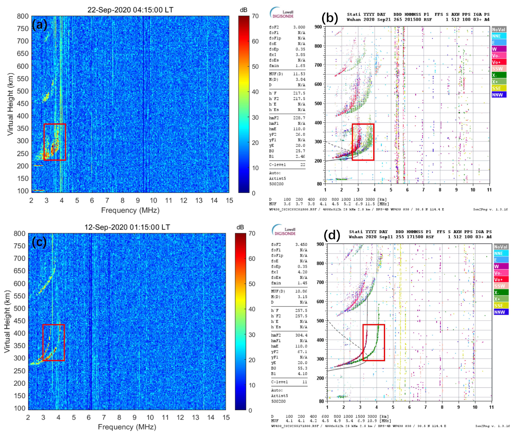
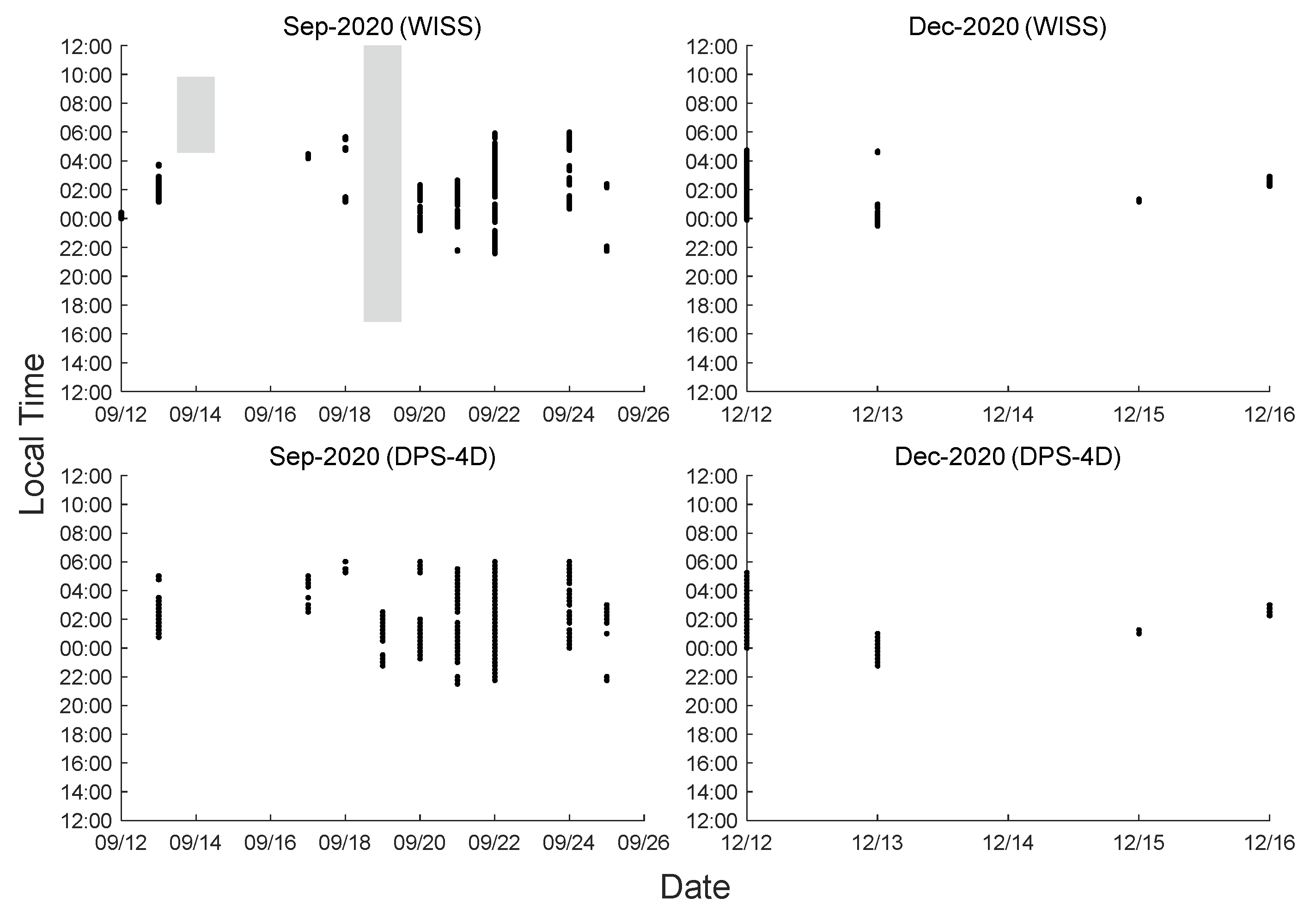
2. Data and Methodology

The ionospheric data used in this study are recorded by Wuhan Ionospheric Sounder System (WISS) at Zhangye station (39.21°N, 100.54°E, Dip Lat 29.6°N), which was installed jointly by the Ionospheric Laboratory of Wuhan University and the Space Center of Chinese Academy of Sciences in 2016. Data resolution of the ionosonde is 5 min. The ionogram data from 2017 to 2022 were selected, and a detailed distribution of the data is shown in

Table 1. Distribution of ionogram data at Zhangye.

Year	Number of Effective Days	Number of Missing Days	Specific Date of the Missing Data (Day/Month)
2017	335	30	5 June–6 July
2018	343	22	1 February–7 February; 9 February; 12 February–14 February; 18 March–20 March; 14 April–18 April; 28 April–30 April
2019	365	0
2020	343	23	22 November–14 December
2021	361	4	28 March–31 March
2022	360	5	11 June–15 June

. A software tool, ionoScaler v2.0 [19], was used to manually scale ionograms. Moreover, ionograms recorded by DPS-4D [20] at Beijing station (40.25°N, 116.25°E, Dip Lat 30.9°N) in 2018 were used to compare with observations at Zhangye station in this study. Figure 1 shows the geographical location of Zhangye and Beijing stations, where Zhangye station is at the edge of the Qinghai-Tibet Plateau. The data of solar 10.7 fluxes and Ap index used in this study was downloaded from ftp://ftp.gfzpotsdam.de/pub/home/obs/Kp_ap_A p_SN_F107 (accessed on 21 March 2023).

To study the effects of different systems on SF observations, a comparison of the data from WISS and DPS-4D at Wuhan station on several days in 2020 was carried out. There are several differences between WISS and DPS-4D. The DPS-4D is equipped with a dual-channel receiver, whereas WISS features a single-channel receiver which cannot separate O-waves and X-waves. Data resolution of DPS-4D is 15 min, and the antennas of the two ionosondes are also different. The elevation of antennas can affect returned echoes from different positions in the ionosphere over the transmitter and then lead to some slightly different echoes on ionograms. Therefore, to test the difference of observations from these two ionosondes, Figure 2 shows ionograms recorded by WISS and DPS-4D at Wuhan. We marked ionograms with SF according with the Handbook of Ionogram Interpretation and Reduction [21], with the red rectangles marking the trace of the F2 layer. For the operator, Figure 2a,b was identified as SF, however, there are no SF for Figure 2c,d. To further study the differences between these two systems, Figure 3 shows the comparison of SF observations on some days in September and December in 2020. The black bars indicate the occurrences of SF events and grey parts indicate the data missed in Figure 3. The two digital ionosondes have similar results for SF observation.

In this study, the occurrence rate of SF is calculated by Equation (1).

$$P\left(Y,M,LT\right)=\frac{n(Y,M,LT)}{N(Y,M,LT)}\times 100\%$$

(1)

where $Y$ (Year) = 2017–2022, $M$ (Month) = 1–12, $LT$ (local Time) = 1–24, $n$ is the number of SF occurrences at $LT$-th time of the $M$-th month of $Y$-th year. $N$ is the number of ionograms recorded by the ionosonde in the corresponding time.

3. Result

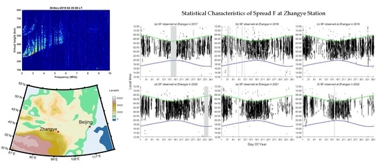
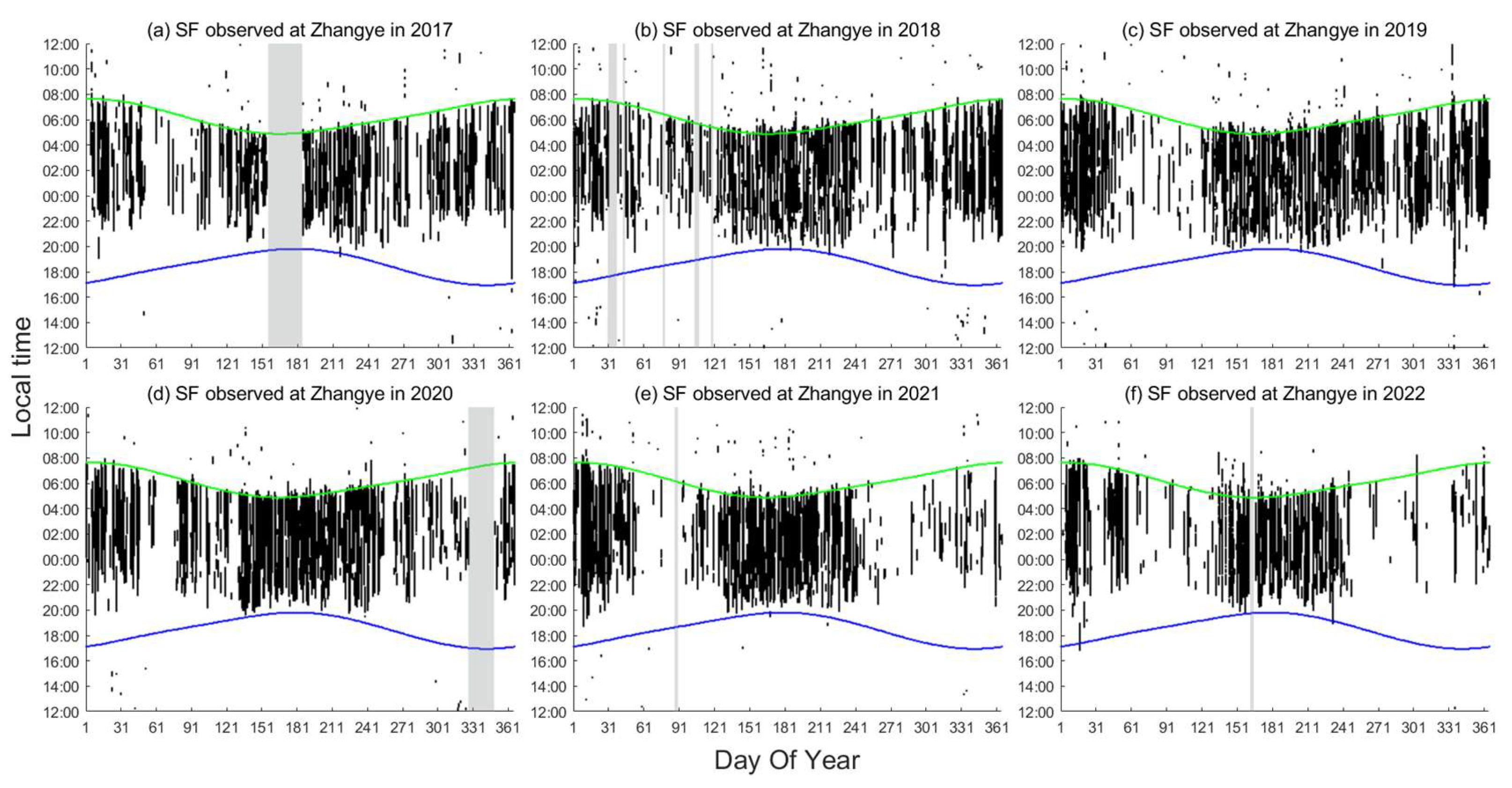
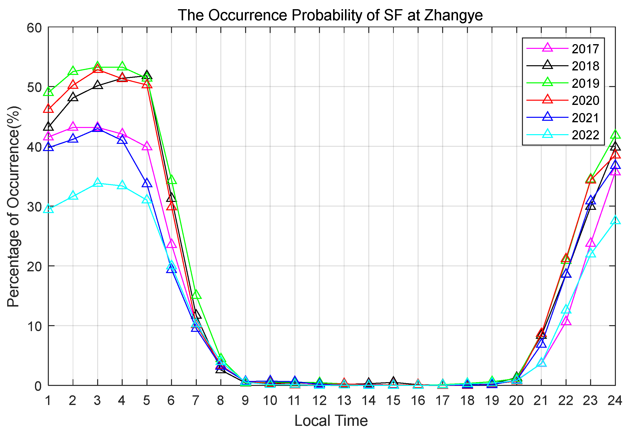
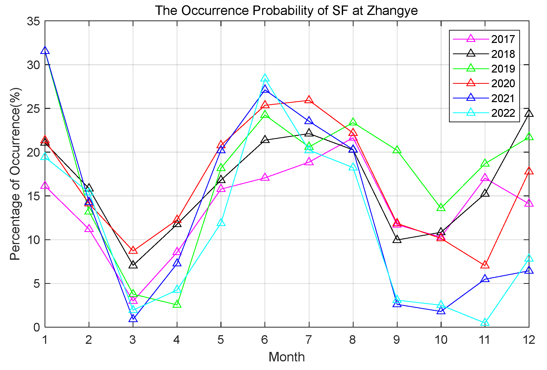
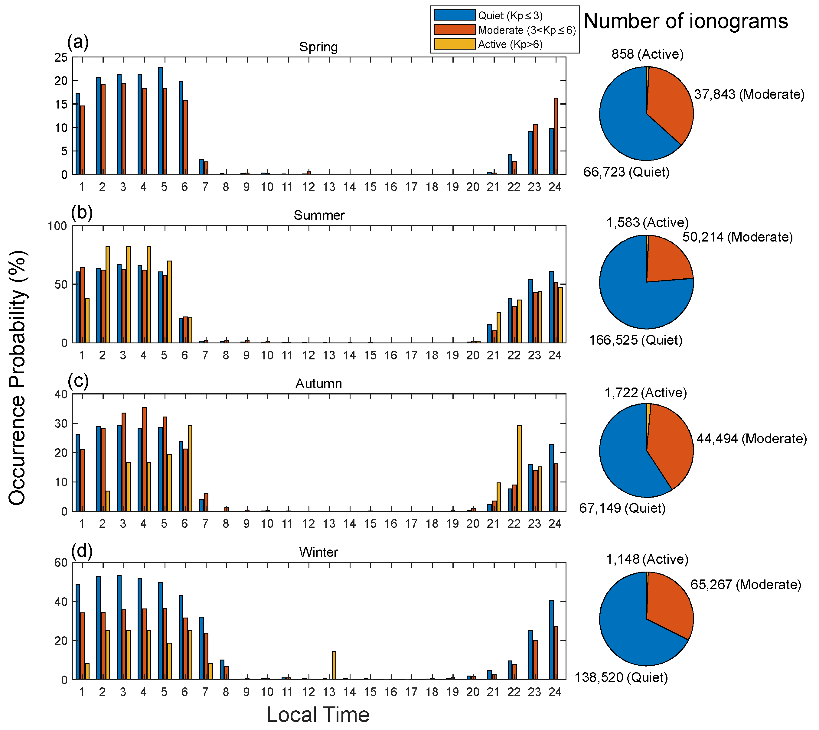
3.1. Diurnal and Seasonal Variations of Spread F

In this study, SF has not been categorized to establish different types, but instead to distinguish whether it occurs or not. Figure 4 shows variations of SF as a function of local time and day of year. The x-axis is the day of the year, and the y-axis represents the local time of day. Similar to Figure 3, the grey parts in Figure 4 indicate the missed data and the black bars indicate the occurrence of SF events. The green and blue lines in Figure 4 indicate the local time of sunrise and sunset, respectively. It can be seen from Figure 4 that SF events occurred almost every day. Results are similar with the occurrence of SF in Moscow (55.5°N, 37.3°E) [12]. It can be found that the effect of solar terminator on SF is more evident at the sunrise time than sunset time except summer, which is similar as the results over Nicosia (35.19°N, 33.38°E) [12]. It can be seen from Figure 4 that SF can be observed occasionally during daytime. However, in this study, we focused on the characteristics of nighttime SF.

Figure 5 shows an average probability of the occurrence of SF at different local times from 2017 to 2022. It can be seen from Figure 5 that the maximum of the occurrence probability is around post-midnight. Moreover, for the effect of solar activity, the maximum value of the occurrence is during the low solar activity years (2018–2020). The diurnal variations of SF are similar to observations made by Huang et al. [11]. However, compared with observations over other mid-latitude stations (maximum values were around 16% at Changchun (43.8°N, 125.3°E) and around 9% at Urumqi (43.7°N, 87.6°E) [11]), the occurrence probabilities of SF in this study are much higher. They are 43.2% (2017, between 01 LT to 02 LT), 51.8% (2018, between 04 LT to 05 LT), 53.3% (2019, between 02 LT to 03 LT), 53.0% (2020, between 02 LT to 03 LT), 43.0% (2021, between 02 LT to 03 LT) and 33.8% (2022, between 02 LT to 03 LT), respectively.

In this study, one year was divided into four seasons: spring (months 3–4), summer (months 5–8), autumn (months 9–10) and winter (months 11–12 and 1–2) to study seasonal characteristics of SF. Figure 6 shows seasonal variations of SF. It was found that the occurrence rate of SF in each year almost has similarly seasonal characteristics. In winter and summer, SF has a higher occurrence rate, while the occurrence probability of SF is relatively lower in spring and autumn. The greatest differences are in autumn and winter. It can be found that the occurrence rate of SF in 2021 and 2022 are lower than other years in autumn and winter (especially in early winter), while the occurrence probability in 2019 is much higher. The monthly occurrence probabilities of SF from 2017 to 2022 are in the range of 2.98–21.63% (2017), 8.82–22.12% (2018), 2.54–31.54% (2019), 7.04–25.92% (2020) and 0.88–31.53% (2021) and 0.48–28.40% (2022), respectively. It is interesting that the maximal values of monthly probabilities are in January in 2019 and 2021, which are not similar with other years.

Figure 7 presents the occurrence probabilities of SF as a function of local time and month from 2017 to 2022. In summer, the occurrence probabilities of SF can reach approximately 80% or higher. The occurrence probability of SF is higher during nighttime in summer and winter but lower in spring and autumn. The occurrence rates of SF are very low in March during 2021 and 2022. The maximum rates of each year are around the midnight in summer and the secondary peak value appeared around the midnight in winter, but opposite in 2019. Guo et al. [13] shows similar characteristics of SF over Changchun and Urumqi and the occurrence probabilities have a similar pattern but with a lower level (less than 45%).

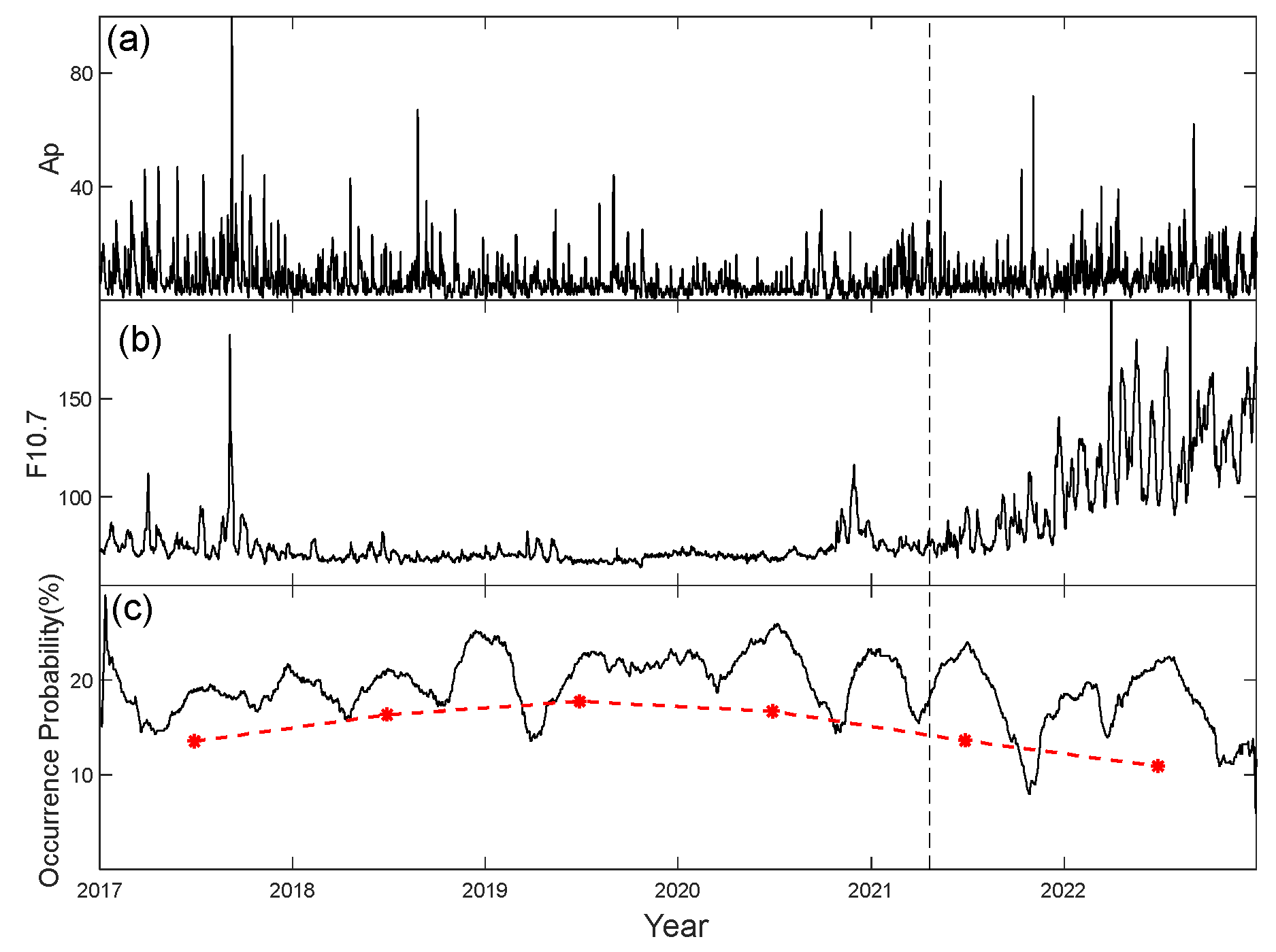
3.2. Dependence of Solar and Geomagnetic Activity

In order to study the correlation between SF and solar activity, Figure 8b,c show the solar radio fluxes at 10.7 cm (F10.7) and daily probability of SF from 2017 to 2022 (the probability curve has been smoothed). The Ap index is also drawn for a more comprehensive analysis (Figure 8a). In Figure 8c, the red dotted line indicates the average annual probability of SF. It is found from Figure 8 that the occurrence probability value decreases when the F10.7 increases.

It can be seen in Figure 6 that the occurrence rates of SF are lower in spring and autumn compared to other seasons. However, there are some slight differences. Therefore, to further analyze the effect of solar activity on the SF, Figure 9 shows the diurnal variation of SF in different seasons in 2019 and 2022. It can be seen from Figure 9 that the occurrence probabilities of SF are both high in summer of these two years. However, the occurrence probability of SF in 2019 is higher than 2022 in autumn and winter.

Recent studies show that during geomagnetic disturbed periods equatorial plasma bubbles can reach mid-latitudes [8,22]. To study the effect of geomagnetic activity on the occurrence of SF, Figure 10 shows the distribution of the occurrence rates of SF with local time and geomagnetic activity in different seasons during 2017–2022. The color bars indicate occurrence rates under geomagnetic quiet (blue), moderate (orange) and active (yellow) conditions, and the pie chart (right panel) represents the corresponding number of ionograms. The maximum value of Kp on the very day was used to represent geomagnetic activity. In spring, it can be seen from Figure 10 that there is no positive relationship between geomagnetic activity and the occurrence of SF during 00:00 LT to 06:00 LT. However, there are some slightly positive relationships during 22:00 LT to 24:00 LT. In summer, the occurrence rate of SF increased during the post-midnight period under geomagnetically active condition. There are no positive effects on SF during the pre-midnight period. In autumn, the occurrence rate of SF is slightly higher under the geomagnetic moderate and active conditions than the quiet condition during 03:00 LT to 06:00 LT (21:00 LT to 22:00 LT). In winter, there are no positive effects on SF at nighttime during geomagnetically active condition. Previous studies [23,24,25] found that there is a negative relationship between SF and geomagnetic activity. However, Su et al. [26] suggested that the occurrence of mid-latitude irregularities is not affected by the magnetic condition. The present study further suggests that the relationship between SF and geomagnetic condition might depend on the season and local time.

4. Discussion

Results in this study show that the diurnal, seasonal and solar activity characteristics of SF at Zhangye stations are similar to previous statistical studies at mid-latitude regions [11,14,25]. Wang et al. [14] studies characteristics of SF at Beijing (39.6°N, 116.3°E) and Kezhou (39.7°N, 76.2°E) station in China. The latitudes of these two stations are close to Zhangye station. Reasonably, diurnal variations are similar at these three stations. However, the maximum probabilities of SF at Beijing and Kezhou (both around 22% in 2011) were lower than Zhangye (around 33.83% in 2022) during the high solar activity.

In terms of seasonal variations, similar to previous studies at mid-latitude stations [11,13,14,15], there are double peaks (in summer and winter) on the occurrence probabilities of SF. However, the occurrence rate of SF at Zhangye station is much higher than other mid-latitude stations, especially in winter. The maximum values are around 12% and 15% in winter and summer (Beijing and Kezhou, 2011) while the corresponding peak values are around 19.4% and 28.4% at Zhangye (2022). Although the year is different for observations at Beijing (Kezhou) and Zhangye, the level of solar activity is comparable. During the minimum solar activity period (1995–1997), the peak values of local time are 44.1% (38.7%) in winter and 30.1% (26.7%) in summer at Changchun (Urumqi), however, the corresponding peak values at Zhangye during the minimum solar activity period (2017–2019) are above 60% and 70% in winter and summer, respectively.

Figure 11 shows comparison of the occurrence probability between Zhangye and Beijing stations in 2018. The solid and dotted lines represent the occurrence probability of SF at Beijing and Zhangye stations. At Beijing station, the occurrence probability in 2011 [14] is comparable with that of 2018. Figure 11a shows that the maximum occurrence probability of SF at Beijing is approximately 30.3% and lower than that at Zhangye (approximately 51.8%). The maximum values are both located between 04:00 LT to 05:00 LT at Beijing and Zhangye stations. The occurrence probabilities at Zhangye are higher than which at Beijing for all local times. In Figure 11b, the occurrence probability of SF at Beijing is in the range of 2.2–22.3% and the trend of seasonal variation is similar with Zhangye. It also can be seen from Figure 11b that the occurrence probabilities are comparable at Zhangye and Beijing in spring and summer seasons. However, in autumn and winter, they are much higher at Zhangye than Beijing.

In mid-latitude regions, there is an electrodynamical coupling process between E and F regions in the ionosphere [7,27] which might affect the occurrence of SF. Zhou et al. [28] analyzed the occurrences of Es layers and SF over Wuhan and found that there is a positive relationship between diffused Es and SF during nighttime. Interestingly, Wang et al. [29] studied the Es layer over Zhangye and Beijing stations in 2018. The statistical results show the occurrence probabilities of Es at Zhangye are higher than that at Beijing, especially in autumn and winter. However, the occurrence of Es in winter is much lower than that in summer at Zhangye station. On the other hand, the different occurrence rates of Es between Beijing and Zhangye stations is not as large as that for SF. Therefore, the E-F region coupling cannot explain the high occurrence rate of SF at Zhangye station. Wang et al. [29] concluded that gravity waves might play an important role on the formation of the Es layer. At the same location, it is reasonable to consider that gravity waves might be a main driver for the abnormal high probabilities of SF in autumn and winter.

Gravity waves can play an important role on the occurrence of SF at middle latitudes over recent decades. The neutral particle density perturbations induced by gravity waves are usually considered as a seeding source of SF. Kelley [30] proposed that gravity waves created a finite structure firstly then were amplified by plasma instability, which cause ionospheric irregularities. Bowman [31] suggested that seasonal variation of SF might be associated with neutral particle density. Results show that there is a negative relationship between the occurrence of SF and neutral particle density in the upper atmosphere. Hines [32] found that the amplitude of gravity waves increased with a low neutral particle density, therefore, gravity waves may play key roles on seasonal variation of SF. Furthermore, gravity waves mainly originate in the lower atmosphere and are greatly affected by the topographic conditions. Compared with the plain region [33], gravity waves in the plateau region can propagate up to a higher altitude.

Wan et al. [18] statistically analyzed the traveling ionospheric disturbance above the Qinghai-Tibet Plateau and suggested that TIDs might be related to the special topography. According to the observational results by Wan et al. [18], TIDs observed in central China mainly propagated in the northeastward and southeastward direction. The two sources of TIDs were right in the southeastern and northeastern edges of the Qinghai-Tibet Plateau. Because of the tropospheric westerlies, there are a lot of vortexes in lee side which might excite gravity waves [34]. Coincidentally, Zhangye station is just located at the northeastern edge of the Qinghai-Tibet Plateau. The effects of gravity waves are long-lasting because of the unchanging topography. Therefore, the high occurrence probabilities of SF at Zhangye may be attributed to the presence of strong gravity waves.

In terms of seasonal variations, there are some seasonal abnormalities of SF at Zhangye station. During the autumn and winter periods from 2017 to 2020, the occurrence probabilities of SF events at Zhangye are comparable to, if not higher than, the occurrences in summer. Notably, the probabilities in winter are higher than that in summer for the year of 2019 and 2021. Figure 3 in Wan et al. [18] studied seasonal characteristics of TID sources and tropospheric vortexes and found that TID sources in the southeastern and northeastern edge of the Qinghai-Tibet Plateau occurred mainly in autumn and winter. It is well known that mid-latitude SF is mainly caused by TIDs [4,5]. Moreover, TIDs are the manifestation of gravity waves in the ionosphere [1,35,36]. To further study the relationship between SF and TIDs/gravity waves, Figure 12 shows variations of the virtual heights at various frequencies on some typical days (15 January, 11 March and 12 October in 2017 and 18 January in 2019). The black lines in Figure 12 indicate the downward movement of the phase velocity of TIDs in the ionosphere, and gray parts represent the duration of SF. TIDs can occur frequently during the occurrence of SF. To show ionospheric disturbances in different months, the virtual height histograms of monthly mean of ionograms have been drawn by image projection technique [37,38,39] as Figure 13. For virtual height histograms of ionograms, we sum up all pixels including noise for all frequencies at each height on ionograms, and then we can get the height histogram of ionograms along the height. A virtual height-time display is obtained by converting the height histogram into a single vertical line and plotting this line obtained from each successive ionogram as a function of time [39]. January, December, March and October were selected to represent winter, spring and autumn, respectively. Compared with observations in other regions, the occurrence rates of SF are mostly similar in summer. This study focused on the abnormal phenomena of the occurrence rate in spring, autumn and winter. Therefore, the summer months were not shown in Figure 13. The maximum values marked by black lines are close to the base virtual height of ionograms. Virtual height increases are associated with wave-like structures in the ionosphere. It is well known that wave-like structures in the ionosphere are associated with gravity waves [4]. Therefore, the disturbances of black curves can represent ionospheric disturbances. In this study, ionospheric disturbances during the pre-midnight period are considered (red rectangles in Figure 13). It can be seen from Figure 13 that the black lines changed slightly in March (red rectangles) and dramatically in the other three months, indicating the fact that ionospheric disturbances are stronger in autumn and winter at Zhangye. In other words, gravity waves at Zhangye station are more active in these two seasons. Therefore, more active gravity waves can cause higher occurrence rate of SF in autumn and winter, which further lead to seasonal abnormalities of SF. The results of Wang et al. [29] showed a small difference in the occurrence probabilities of Es layer between Zhangye and Beijing in summer, however, the occurrence probabilities of Es are higher (around 10%) at Zhangye station than Beijing in autumn and winter. In Figure 11b, seasonal variation of the occurrence probability of SF has the similar trend with the Es. The power spectrum of gravity waves in the Qinghai-Tibet Plateau are stronger in midnight [40], which might result in a larger effect of gravity waves on SF than on Es. In autumn and winter of 2021 and 2022, especially for 2022, the occurrence probabilities are lower than other years, which might be because of solar activity. It is apparent that solar activity become more active since the latter half of 2021 (Figure 8) in autumn and winter. Gravity waves might vary with solar activity. Vadas [41] suggested that gravity waves have larger amplitudes at F region during the minimum solar activity but at higher altitudes during the maximum solar activity. Liu et al. [42] found a significant negative response between gravity waves and F10.7. As a result, the solar activity has a significant effect on the occurrence of SF in autumn and winter. However, the occurrence probabilities of SF in summer (and spring) are similar in this study and seem to not be influenced by solar activity. Paul et al. [12] also showed that there is no negative dependence of solar activity in summer and equinox period over Nicosia from 2009 to 2020, however, the physical mechanism is still not clear. It is reasonable to think that gravity waves might not be active in spring and summer. As a result, the effect of solar activity cannot be shown in the occurrence of SF in summer and spring.

5. Conclusions

In this study, we carried out statistical analysis of spread F recorded at Zhangye station in the mid-latitude region of China. The data are recorded from 2017 to 2022, which cover half of a solar cycle. In addition, comparisons of SF at Zhangye and Beijing stations were conducted. The main results can be summarized as follows:

(1)

Statistical results show that the diurnal, seasonal and solar activity variations are consistent with previous studies. The maximum occurrence rates of SF are mostly during post-midnight. As for seasonal variation, the occurrence probabilities of SF are higher in summer and winter, and the highest value is in summer (except 2019). In this study, there is a negative relationship between solar activity and SF. However, the relationship between SF and geomagnetic condition might depend on the specified season and local time.

(2)

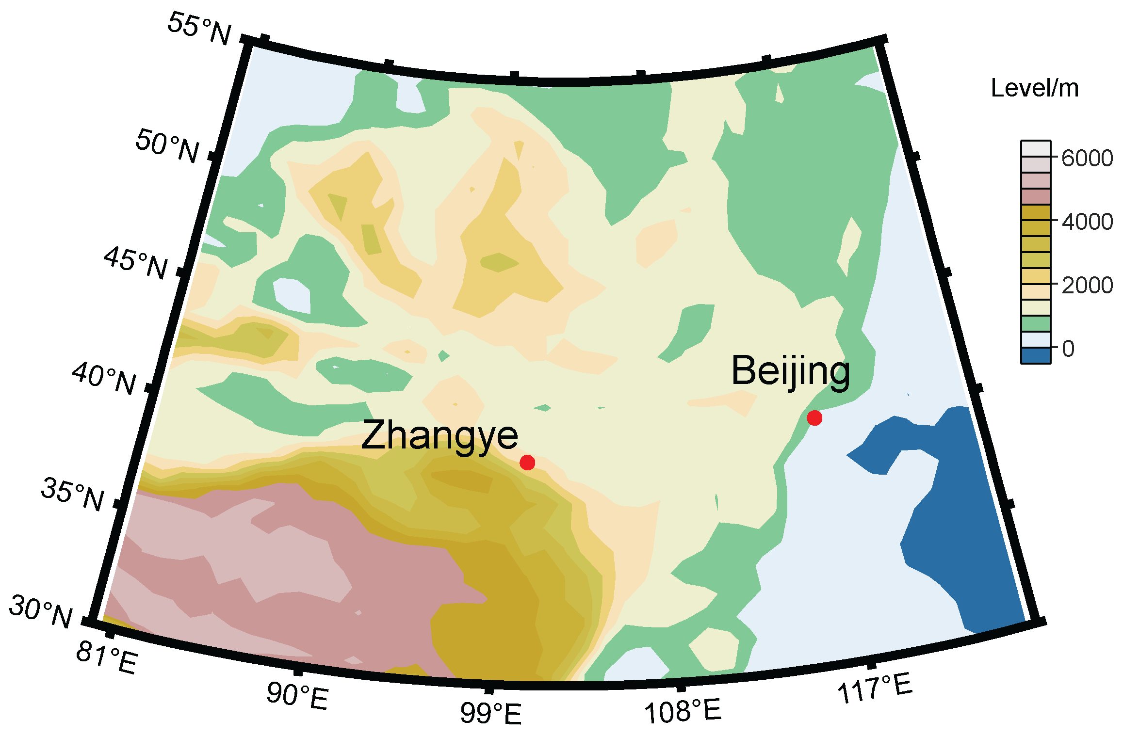
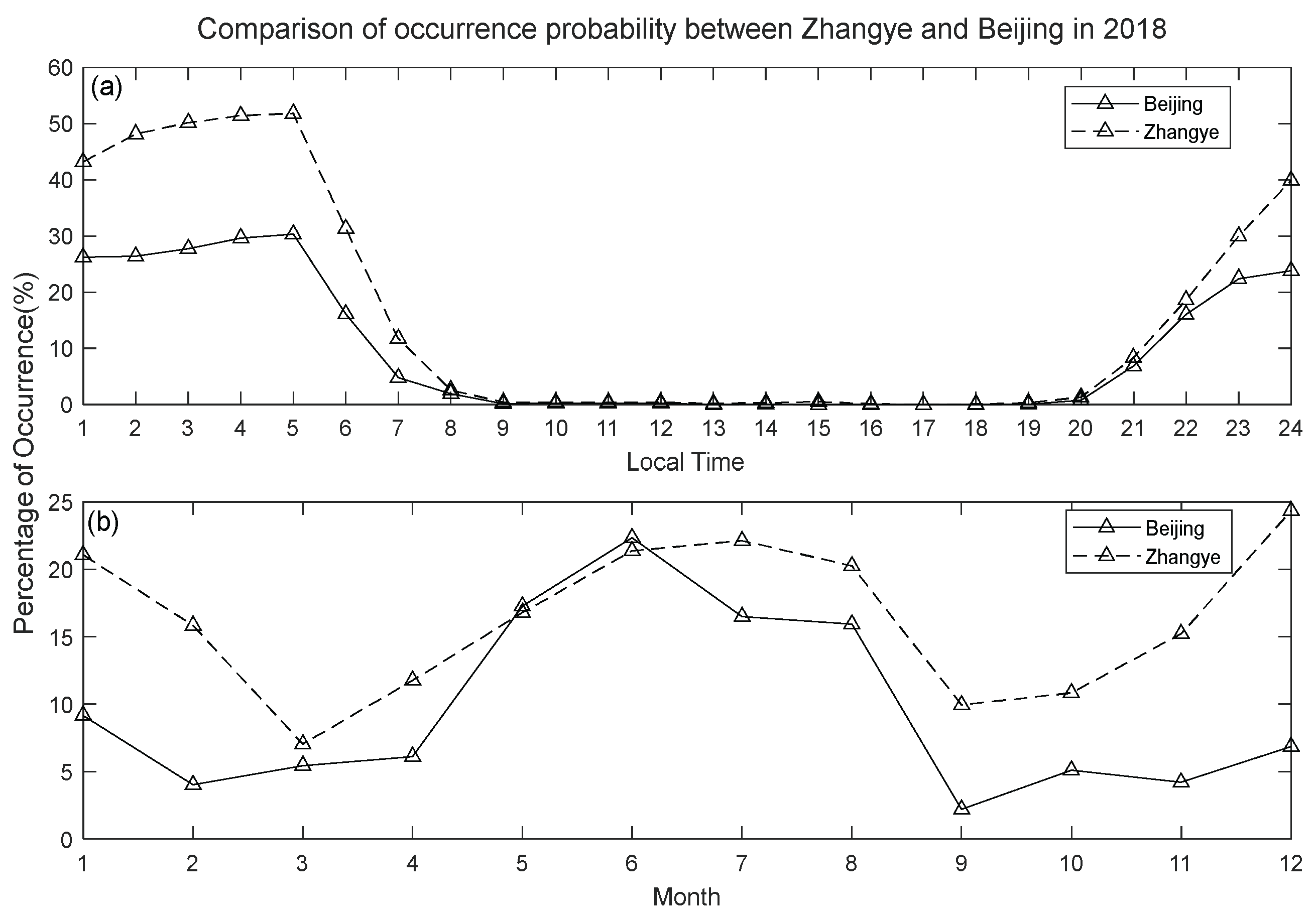
We found that there are several anomalies for the occurrence rate of SF in this study. First, the occurrence probabilities of SF are higher than other mid-latitude stations (Beijing station). Second, the occurrence probabilities of SF are abnormal higher in autumn and winter from 2017 to 2020, but lower in 2021 and 2022 (except January 2021).

(3)

The anomalies mentioned above might be attributed to gravity waves in the northeast of the Qinghai-Tibet Plateau and the effect of solar activity. Gravity waves in the Qinghai-Tibet Plateau are more active in autumn and winter which might cause the higher occurrence probability of SF. The solar activity might have an influence on gravity waves, which lead to the lower occurrence probabilities of SF in 2021 and 2022.

References

1. Abdu, M.A.; Muralikrishna, P.; Batista, I.S.; Sobral, J.H.A. Rocket observation of equatorial plasma bubbles over Natal, Brazil, using a high-frequency capacitance probe. J. Geophys. Res. Space Phys. 1991, 96, 7689–7695. [Google Scholar] [CrossRef]
2. Booker, H.G.; Wells, H.W. Scattering of radio waves by the F-region of the ionosphere. Terr. Magn. Atmos. Electr. 1938, 43, 249–256. [Google Scholar] [CrossRef]
3. Perkins, F. Spread F and ionospheric currents. J. Geophys. Res. 1973, 78, 218–226. [Google Scholar] [CrossRef]
4. Bowman, G.G. A review of some recent work on mid-latitude spread-F occurrence as detected by ionosondes. J. Geomagn. Geoelectr. 1990, 42, 109–138. [Google Scholar] [CrossRef]
5. Paul, K.S.; Haralambous, H.; Oikonomou, C.; Singh, A.K.; Gulyaeva, T.L.; Panchenko, V.A.; Altadill, D.; Buresova, D.; Mielich, J.; Verhulst, T. Mid-latitude spread F over an Extended European area. J. Atmos. Sol. Terr. Phys. 2023, 248, 106093. [Google Scholar] [CrossRef]
6. Xu, S.; Yue, J.; Xue, X.; Vadas, S.L.; Miller, S.D.; Azeem, I.; Straka, W., III; Hoffmann, L.; Zhang, S. Dynamical coupling between Hurricane Matthew and the middle to upper atmosphere via gravity waves. J. Geophys. Res. Space Phys. 2019, 124, 3589–3608. [Google Scholar] [CrossRef]
7. Kelley, M.C.; Haldoupis, C.; Nicolls, M.J.; Makela, J.J.; Belehaki, A.; Shalimov, S.; Wong, V.K. Case studies of coupling between the E and F regions during unstable sporadic-E conditions. J. Geophys. Res. 2003, 108, 1447. [Google Scholar] [CrossRef]
8. Jiang, C.; Wei, L.; Yang, G.; Aa, E.; Lan, T.; Liu, T.; Liu, J.; Zhao, Z. Large-Scale Ionospheric Irregularities Detected by Ionosonde and GNSS Receiver Network. IEEE Geosci. Remote Sens. Lett. 2021, 18, 940–943. [Google Scholar] [CrossRef]
9. Paulikas, G.A. Precipitation of particles at low and middle latitudes. Rev. Geophys. 1975, 13, 709–734. [Google Scholar] [CrossRef]
10. Dabas, R.S.; Das, R.M.; Sharma, K.; Garg, S.C.; Devasia, C.V.; Subbarao, K.S.V.; Rama, R.P.V.S. Equatorial and low latitude spread-F irregularity characteristics over the Indian region and their prediction possibilities. J. Atmos. Sol. Terr. Phys. 2007, 69, 685–696. [Google Scholar] [CrossRef]
11. Huang, W.Q.; Xiao, Z.; Xiao, S.G.; Zhang, D.H.; Hao, Y.Q.; Suo, Y.C. Case study of apparent longitudinal differences of spread F occurrence for two midlatitude stations. Radio Sci. 2011, 46, 1–8. [Google Scholar] [CrossRef]
12. Paul, K.S.; Haralambous, H.; Singh, A.K.; Gulyaeva, T.L.; Panchenko, V.A. Mid-latitude Spread F long-term occurrence characteristics as a function of latitude over Europe Adv. Space Res. 2022, 70, 710–722. [Google Scholar] [CrossRef]
13. Guo, B.; Xiao, S.G.; Shi, J.K.; Xiao, Z.; Wang, G.J.; Cheng, Z.W.; Shang, S.P.; Wang, Z.; Suo, Y.C. Comparative study on characteristics of spread-F at low and mid-latitudes during high and low solar activities over East Asia. Chinese J. Geophys. 2017, 60, 3289–3300. (In Chinese) [Google Scholar]
14. Wang, Y.G.; Mao, T.; Lü, J.; Mei, D. Characteristics of spread-F occurrence in China region in low solar cycle. Prog. Geophys. 2020, 35, 0050–0054. (In Chinese) [Google Scholar] [CrossRef]
15. Igarashi, K.; Kato, H. Solar Cycle Variations and Latitudinal Dependence on the Mid-Latitude Spread-F Occurrence around Japan; XXIV General Assembly: Kyoto, Japan, 1993. [Google Scholar]
16. Paul, K.S.; Haralambous, H.; Oikonomou, C.; Paul, A.; Belehaki, A.; Ioanna, T.; Kouba, D.; Buresova, D. Multi-station investigation of spread F over Europe during low to high solar activity. J. Space Weather Space Clim. 2018, 8, A27. [Google Scholar] [CrossRef]
17. Bhaneja, P.; Earle, G.D.; Bishop, R.L.; Bullett, T.W.; Mabie, J.; Redmon, R. A statistical study of midlatitude spread F at Wallops Island, Virginia. J. Geophys. Res. 2009, 114, A04301. [Google Scholar] [CrossRef]
18. Wan, W.; Yuan, H.; Ning, B.; Liang, J.; Ding, F. Traveling ionospheric disturbances associated with the tropospheric vortexes around Qinghai-Tibet Plateau. Geophys. Res. Lett. 1998, 25, 3775–3778. [Google Scholar] [CrossRef]
19. Jiang, C.; Yang, G.; Zhou, Y.; Zhu, P.; Lan, T.; Zhao, Z.; Zhang, Y. Software for scaling and analysis of vertical incidence ionograms-ionoScaler. Adv. Space Res. 2017, 59, 968–979. [Google Scholar] [CrossRef]
20. Reinisch, B.W.; Galkin, I.A.; Khmyrov, G.M.; Kozlov, A.V.; Lisysyan, I.A.; Bibl, K.; Cheney, G.; Kitrosser, D.F.; Stelmash, S.; Roche, K.; et al. Advancing Digisonde technology: The DPS-4D, in Radio Sounding and Plasma Physics. AIP Conf. Proc. 2008, 974, 127–143. [Google Scholar] [CrossRef]
21. Piggott, W.R.; Rawer, K.U.R.S.I. Handbook of Ionogram Interpretation and Reduction; World Data Center A for Solar-Terrestrial Physics NOAA: Boulder, CO, USA, 1972; pp. 17–18. [Google Scholar]
22. Katamzi-Joseph, Z.T.; Habarulema, J.B.; Hernández-Pajares, M. Midlatitude postsunset plasma bubbles observed over Europe during intense storms in April 2000 and 2001. Space Weather 2017, 15, 1177–1190. [Google Scholar] [CrossRef]
23. Chandra, H.; Rastogi, R.G. Equatorial spread-F over a solar cycle. Ann. Geophys. 1972, 28, 709–716. [Google Scholar]
24. Bowman, G.G. Short-term delays in ionogram-recorded equatorial spread F occurrence of equatorial spread F. Ann. Geophys. 1995, 11, 624–663. [Google Scholar]
25. Wang, G.J.; Shi, J.K.; Wang, X.; Shang, S.P.; Zherebtsov, G.; Pirog, O.M. The statistical properties of spread F observed at Hainan station during the declining period of the 23rd solar cycle. Ann. Geophys. 2010, 28, 1263–1271. [Google Scholar] [CrossRef]
26. Su, S.Y.; Liu, C.H.; Ho, H.H.; Chao, C.K. Distribution characteristics of topside ionospheric density irregularities: Equatorial versus midlatitude regions. J. Geophys. Res. 2006, 111, A06305. [Google Scholar] [CrossRef]
27. Cosgrove, R.B.; Tsunoda, R.T. Instability of the E-F coupled nighttime midlatitude ionosphere. J. Geophys. Res. 2004, 109, A04305. [Google Scholar] [CrossRef]
28. Zhou, C.; Tang, Q.; Huang, F.; Liu, Y.; Gu, X.; Lei, J.; Ni, B.; Zhao, Z. The simultaneous observations of nighttime ionospheric E region irregularities and F region mediumscale traveling ionospheric disturbances in midlatitude China. J. Geophys. Res. Space Phys. 2018, 123, 5195–5209. [Google Scholar] [CrossRef]
29. Wang, W.; Jiang, C.; Wei, L.; Tang, Q.; Huang, W.; Shen, H.; Liu, T.; Yang, G.; Zhou, C.; Zhao, Z. Comparative Study of the Es Layer between the Plateau and Plain Regions in China. Remote Sens. 2022, 14, 2871. [Google Scholar] [CrossRef]
30. Kelley, M.C.; Fukao, S. Turbulent upwelling of the mid-latitude ionosphere: 2. Theoretical framework. J. Geophys. Res. 1991, 96, 3747–3753. [Google Scholar] [CrossRef]
31. Bowman, G.G. Spread-F in the ionosphere and the neutral particle density of the upper atmosphere. Nature 1964, 201, 564–566. [Google Scholar] [CrossRef]
32. Hines, C.O. The upper atmosphere in motion. Q. J. R. Meteorol. Soc. 1963, 89, 1–42. [Google Scholar] [CrossRef]
33. Zeng, X.; Xue, X.; Dou, X.; Liang, C.; Jia, M. COSMIC GPS observations of topographic gravity waves in the stratosphere around the Tibetan Plateau. Sci. China Earth Sci. 2017, 60, 188–197. [Google Scholar] [CrossRef]
34. Medvedev, A.S.; Gavrilov, N.M. The nonlinear mechanism of gravity wave generation by meteorological motions in the atmosphere. J. Atmos. Terr. Phys. 1995, 57, 1221–1231. [Google Scholar] [CrossRef]
35. Mandal, S.; Pallamraju, D.; Karan, D.K.; Phadke, K.A.; Singh, R.P.; Suryawanshi, P. On deriving gravity wave characteristics in the daytime upper atmosphere using radio technique. J. Geophys. Res. Space Phys. 2019, 124, 6985–6997. [Google Scholar] [CrossRef]
36. Kotake, N.; Otsuka, Y.; Ogawa, T.; Tsugawa, T.; Saito, A. Statistical study of medium-scale traveling ionospheric disturbances observed with the GPS networks in Southern California. Earth Planet Spaces 2007, 59, 95–102. [Google Scholar] [CrossRef]
37. Igi, S.; Minakoshi, H.; Yoshida, M. Automatic ionogram processing system. II: Automatic ionogram scaling. J. Commun. Res. Lab. 1992, 39, 367–379. [Google Scholar]
38. Jiang, C.; Yang, G.; Zhao, Z.; Zhang, Y.; Zhu, P.; Sun, H. An automatic scaling technique for obtaining F2 parameters and F1 critical frequency from vertical incidence ionograms. Radio Sci. 2013, 48, 739–751. [Google Scholar] [CrossRef]
39. Lynn, K.J. Histogram-based ionogram displays and their application to autoscaling. Adv. Space Res. 2018, 61, 1220–1229. [Google Scholar] [CrossRef]
40. Qian, T.; Zhang, F.; Wei, J.; He, J.; Lu, Y. Diurnal Characteristics of Gravity Waves over the Tibetan Plateau in 2015 Summer Using 10-km Downscaled Simulations from WRF-EnKF Regional Reanalysis. J. Atmos. 2020, 11, 631. [Google Scholar] [CrossRef]
41. Vadas, S.L. Horizontal and vertical propagation and dissipation of gravity waves in the thermosphere from lower atmospheric and thermospheric sources. J. Geophys. Res. 2007, 112, A06305. [Google Scholar] [CrossRef]
42. Liu, X.; Yue, J.; Xu, J.; Garcia, R.R.; Russell, J.M., III; Mlynczak, M.; Wu, D.L.; Nakamura, T. Variations of global gravity waves derived from 14 years of SABER temperature observations. J. Geophys. Res. Atmos. 2017, 122, 6231–6249. [Google Scholar] [CrossRef]
Figure 1. Locations of Zhangye (39.21°N, 100.54°E, Dip Lat 29.6°N) and Beijing (40.25°N, 116.25°E, Dip Lat 30.9°N) stations.
Remotesensing 16 01142 g001
Figure 2. Ionograms recorded by WISS and DPS-4D at Wuhan, ionograms with SF (a) (WISS, 22 September 04:15 UTC + 8) and (b) (DPS-4D, 21 September 20:15 UTC), without SF in (c) (WISS, 12 September 01:15 UTC + 8) and (d) (DPS-4D, 11 September 17:15 UTC).
Remotesensing 16 01142 g002
Figure 3. Comparison of SF occurrence over Wuhan between WISS and DPS-4D. Black bars indicate occurrences of SF events and grey parts indicate missed data.
Remotesensing 16 01142 g003
Figure 4. Occurrence of SF as a function of local time and day of year in 2017 (a), 2018 (b), 2019 (c), 2020 (d), 2021 (e) and 2022 (f). Grey parts indicate missed data and black bars indicate occurrences of SF events. Green and blue lines indicate local time of sunrise and sunset.
Remotesensing 16 01142 g004
Figure 5. Diurnal variations of SF at Zhangye in 2017 (pink), 2018 (black), 2019 (green), 2020 (red), 2021 (blue) and 2022 (cyan).
Remotesensing 16 01142 g005
Figure 6. Monthly variations of SF at Zhangye in 2017 (pink), 2018 (black), 2019 (green), 2020 (red), 2021 (blue) and 2022 (cyan).
Remotesensing 16 01142 g006
Figure 7. Occurrence probabilities of SF at Zhangye as a function of local time and month from 2017 to 2022.
Remotesensing 16 01142 g007
Figure 8. Ap Index (a), solar 10.7 fluxes (b) and SF occurrence probabilities (c) from 2017 to 2022. The black vertical dotted line indicates solar 10.7 fluxes increase apparently after that time.
Remotesensing 16 01142 g008
Figure 9. Diurnal variations of SF in different seasons in 2019 (solid line) and 2022 (dotted line).
Remotesensing 16 01142 g009
Figure 10. Distribution of occurrence probabilities of SF with local time and geomagnetic activity in spring (a), summer (b), autumn (c) and winter (d). Pie charts show number of ionograms in different seasons and geomagnetic conditions.
Remotesensing 16 01142 g010
Figure 11. Diurnal (a) and seasonal variations (b) of SF at Zhangye and Beijing stations in 2018.
Remotesensing 16 01142 g011
Figure 12. Variations of virtual heights at various frequencies at Zhangye station during 17:00 LT to 06:00 LT (next day) of several days. Black lines indicate downward movement of phase velocity of TIDs in ionosphere, gray parts represent duration of SF.
Remotesensing 16 01142 g012
Figure 13. Virtual height histogram of monthly mean of ionograms in January, March, October and December from 2017 to 2022.
Remotesensing 16 01142 g013