Technical Note

Effects of Equatorial Plasma Bubbles on Multi-GNSS Signals: A Case Study over South China

1
Planetary Environmental and Astrobiological Research Laboratory (PEARL), School of Atmospheric Sciences, Sun Yat-sen University, Zhuhai 519082, China
2
Key Laboratory of Tropical Atmosphere-Ocean System, Ministry of Education, Zhuhai 519082, China
3
Aerospace Information Research Institute (AIR), Chinese Academy of Sciences (CAS), Beijing 100094, China
4
Mengcheng National Geophysical Observatory, University of Science and Technology of China, Hefei 230026, China
5
CAS Key Laboratory of Geospace Environment, School of Earth and Space Sciences, University of Science and Technology of China, Hefei 230026, China
6
School of Petroleum, China University of Petroleum-Beijing at Karamay, Karamay 834000, China
7
Shanghai Radio Equipment Research Institute, Shanghai 201109, China
*
Author to whom correspondence should be addressed.
Remote Sens. 2024, 16(8), 1358; https://doi.org/10.3390/rs16081358
Submission received: 13 March 2024 / Revised: 9 April 2024 / Accepted: 10 April 2024 / Published: 12 April 2024

Abstract

:
Equatorial plasma bubbles (EPBs) occur frequently in low-latitude areas and have a non-negligible impact on navigation satellite signals. To systematically analyze the effects of a single EPB event on multi-frequency signals of GPS, Galileo, GLONASS, and BDS, all-sky airglow images over South China are jointly used to visually determine the EPB structure and depletion degree. The results reveal that scintillations, or GNSS signal fluctuations, are directly linked to EPBs and that the intensity of scintillation is positively correlated with the airglow depletion intensity. The center of the airglow depletion often corresponds to stronger GNSS scintillation, while the edge of the bubble, which is considered to have the largest density gradient, corresponds to relatively smaller scintillation instead. This work also systematically analyzes the responses of multi-constellation and multi-frequency signals to EPBs. The results show that the L2 and L5 frequencies are more susceptible than the L1 frequency is. For different constellations, Galileo’s signal has the best tracking stability during an EPB event compared with GPS, GLONASS, and BDS. The results provide a reference for dual-frequency signal selection in precise positioning or TEC calculation, that is, L1C and L2L for GPS, L1C and L5Q for Galileo, L1P and L2C for GLONASS, and L1P and L5P for BDS. Notably, BDS-2 is significantly weaker than BDS-3. And inclined geosynchronous orbit (IGSO) satellites have abnormal data error rates, which should be related to the special signal path trajectory of the IGSO satellite.

Graphical Abstract

1. Introduction

Ionospheric irregularities are the main source of fluctuations and degradation in GNSS signal quality. When an electromagnetic wave passes through ionospheric irregularities, the amplitude and phase of the signal flutter up and down violently due to fluctuations in the refractive index, which is called scintillation [1,2]. Fluctuations or even interruptions in signals can lead to tremendous increases in errors in precise point positioning (PPP) or real-time kinematic (RTK) methods [3,4,5,6].
At low latitudes and in equatorial regions, equatorial plasma bubbles (EPBs), which are larger-scale plasma depletion structures developed from the bottom of the F2 layer through Rayleigh–Taylor instability after sunset, are the most common ionospheric irregularities [7,8,9,10]. The interior of an EPB contains various small-scale irregularities due to a cascade of secondary instability processes and pre-reversal enhancement [8,11]. Generally, EPBs can extend thousands of kilometers along magnetic field lines in the north–south direction, drift hundreds to thousands of kilometers in the east–west direction, and reach an apex height of 2500 km [12,13]. The part of the EPB corresponding to the L-band Fresnel scale of 300–400 m will cause enormous degradation in the GNSS signal intensity and loss of lock [14,15].
As one of the first known effects of space weather, the impact of irregularities on GNSS has been observed worldwide [16,17]. As early as 1988, Basu et al. [18] analyzed the global distribution of L-band scintillations. Studies on the Brazilian region showed that scintillation follows the seasonal distribution of EPBs [19,20]. From another perspective, the features of carrier phase cycle slip (CS) and GNSS signals loss of locks (LoLs) over local time, season, spatial distribution, and solar activity dependences closely resemble the characteristics of ionospheric irregularities/EPBs at low latitudes [21,22,23,24,25,26]. Many studies have focused on the spatiotemporal relationship between EPBs and GNSS scintillation in the climatological scale. However, how the detailed center and edge parts of the EPB structure affect GNSS signals, and the relationship between the degree of EPB depletion and the GNSS signal quality, are still not well understood.
As more GNSS frequencies and ranging signals have become available recently, the response of new frequencies/signal types to the ionosphere has been evaluated to some extent. Biswas et al. [27] noted that cycle slips occur more frequently and last longer under strong scintillation (S4 > 0.6) conditions; moreover, GPS L5 is the most robust, and L2 is the least robust for signal tracking. GPS L2 and L5 are likely to experience deeper signal fading than L1 is [28,29]. GNSS signals with lower frequencies are more susceptible to strong scintillations, but the S4 index increases linearly with frequency under weak scintillation, which has been verified for both the GPS L1, L2, and L5, and the BDS B1, B2, and B3 frequencies [30,31]. The type of signal modulation may also affect the scintillation performance, as Galileo E5, which uses Alternative Binary Offset Carrier (AltBOC) modulation, has the smallest noise level [32,33]. Studies have shown that GLONASS L1 is better than L2, and Galileo has the best stability [34,35]. However, there is still a lack of comprehensive and systematic research about the effects of EPBs on multiple GNSS frequencies/signal types.
In the present work, we directly use all-sky airglow images to visually determine the EPB structure and depletion degree, and use GNSS measurements to characterize the corresponding signal quality effects, to investigate the direct correspondence between EPBs and GNSS signals. The responses of multi-constellation and multi-frequency signals to EPBs are comprehensively compared and discussed.

2. Data and Methods

In this study, data from an all-sky airglow imager and a GNSS receiver at Zhuhai (22.35°N, 113.58°E) in southern China are used. The all-sky airglow imager is KEO Sentry 4 monochromatic imager. The imager is equipped with five filters, including a 630 nm filter for imaging the ionospheric density in the F2 region. The 630 nm airglow intensity image is obtained with an exposure time of 60 s and an acquisition interval of 5.8 min. Assuming an airglow height of 300 km, each data grid point is projected onto geographic latitude and longitude coordinates based on the distance and azimuth from the zenith. The radius range of the valid airglow image is approximately 400 km (approximately 120° field of view). To remove interference from background light sources, the average of the previous seven images is subtracted from each image. A negative value in the final airglow image means that the ionospheric density is depleted. Figure 1 shows an example of a post-processed airglow image at 15:24 UT on 3 April 2022. The unit of the post-processed airglow image is the same with the intensity value of the original airglow image (from 0 to 65,536, 16 bit), and we focus on the relative magnitude of airglow value. The characteristics of the EPBs are clear, and the airglow value can be extracted at a fixed location and compared with GNSS observations at the ionospheric pierce point (IPP) location at an effective height of 300 km.
The GNSS receiver is a Septentrio PolaRx5S ionospheric scintillation monitoring receiver (ISMR), which records signal messages from multi-frequency and multi-GNSS constellations; generates carrier phase, pseudorange, and carrier-to-noise ratio measurements with a temporal resolution of 1 s in rinex observation data file; and outputs the S4 scintillation index with a temporal resolution of 60 s. The STEC is obtained from dual-frequency carrier-phase observations and converted to vertical TEC (VTEC) [36]. The differential code bias (DCB) is assumed to be constant daily. The observed TEC is assumed to be equal to the TEC from the IGS ionospheric TEC map, after which the DCB is obtained [37]. Observations with elevation angles less than 20 degrees are discarded to mitigate observation errors. The trend of the daily VTEC variation (VTEC baseline) is obtained by the Savitzky–Golay filter [38], which is a least-squares smoothing filter to filter high-frequency signal components, and the deviation VTEC (dVTEC) is subsequently extracted after removing the trend.
In addition, variations in the loss of phase observation and phase cycle slip (CS) are used to assess the GNSS signal quality. Loss of phase observation is identified as the absence of a recorded carrier phase due to the low signal strength [39]. Moreover, the G-nut Anubis v3.6 tool (https://gnutsoftware.com/, accessed on 1 March 2024) has been used to detect cycle slips [40]. The principles of the cycle slip detection algorithm in G-nut Anubis tool are based on independent linear combinations of triple-frequency undifferenced GNSS observations [41]. Losses of phase and cycle slips are identified as error epochs in this study.
The EPB events on 3 April 2022 are selected, with a mean Kp of 1.75 and F10.7 of 140.2, suggesting quiet geomagnetic conditions.

3. Comparison of GNSS and Airglow Data

All-sky 630 nm airglow images can visually display the morphology and motion state of EPBs [42]. In this section, the combined observations of airglow images and GNSS measurements are used to investigate the detailed influence of the spatial distribution and depletion degree of EPBs on GNSS signals.
Figure 2 shows the comparison results of the airglow depletion, S4 index, and deviation VTEC (dVTEC) for the Galileo and GPS constellations during 12–20 UT on 3 April 2022. Considering that low elevation data may cause positional uncertainty between the GNSS signal path and airglow intensity, we select the observations with the highest elevation angle at each epoch in the airglow image coverage, as shown in Figure 2a,b. Relative airglow values less than 0, which have been discussed in the data processing section, are considered to indicate density depletion (i.e., an EPB) and are manually identified to ensure accuracy. The center of the EPB is with the strongest airglow depletion, while the edge of the EPB is the start and end of the airglow depletion. As shown in Figure 2c,d, when the airglows presented depletions, the S4 scintillation index increased obviously and the dVTEC showed prominent oscillation. Airglow depletions with larger magnitudes generally resulted in greater S4 values and dVTEC oscillations. In addition, when there was no airglow depletion, both the S4 index and dVTEC were relatively low. In Figure 2d, the airglow depletion at 13–14 UT was contaminated by an external light source near nightfall, which made it difficult to calculate the correct airglow depletion value; this value is not shown.
The above results in Figure 2 reflect the relationship between EPBs and scintillation to some extent. However, uncertainties could be introduced from the movement of IPP trajectories of MEO satellites. Due to the orbital design of geostationary orbit (GEO) satellites, the IPP is considered to be in a fixed state, which provides advantageous conditions for further comparison with airglow images [43].
Figure 3 shows a comparison between the airglow depletion, S4 index, and dVTEC observed by GEO satellites. According to the longitude of the IPP, as shown in Figure 3a, the eight GEO satellites are arranged from east to west. The S4 and dVTEC results of the GEO satellites also show good agreement with the airglow depletion, as airglow depletion corresponds to a greater S4 index and stronger dVTEC oscillation. At ~14.5 UT, as shown in Figure 3b–d, the airglow depletion seems to be interrupted, but scintillations still continue to appear. After confirmation from the original airglow image, it is found that this actually corresponds to two separate branch structures of the EPB tens of kilometers apart. The continuous unbroken scintillations may be due to the tilt of the signal path, which causes the signal to pass through the upper or lower part of the EPB, even though the IPP is located between the two branches. Therefore, the duration of airglow depletion is always less than the duration of scintillation because the signal path may pass through the EPB at various heights. The combined observations of airglow images and GEO satellite data clearly reveal the east-to-west zonal motion, depletion evolution, and lifetime of the EPB. Based on the spatial distribution and motion observed from airglow depletion, the core part of the EPB structure generally produced a greater S4 value, while the outer part of the EPB produced a smaller S4 value. For the EPB structure during 16–18 UT in Figure 3b–f and during 17.5–19 UT in Figure 3g,h, the depletion degree of the EPB gradually decreased. Correspondingly, the S4 index value and the dVTEC oscillation decreased. Near the end of the EPB lifetime at ~18 UT in Figure 3e,f or ~18.5 UT in Figure 3g,h, although the airglow still showed obvious depletion, the S4 index and dVTEC only presented slight changes. This might be because the irregularity scale sizes of the EPB changed during different life periods, and the L-band sensitive scale size of 300–400 m might not be dominant near the end of the EPB lifetime.
Benefiting from the almost fixed position of the GEO satellite, joint observations reveal some detailed relationships between EPBs and scintillation. The center of the EPB depletion often corresponds to stronger scintillation, while the edge of the bubble, which is considered to have the largest density gradient, corresponds to relatively smaller scintillation instead. From the perspective of the dVTEC obtained from phase observations, the sharp fluctuations also correspond to the center of the airglow depletion.

4. Signal Quality Assessment

The above results indicate that EPB could induce greater S4 values and TEC oscillations, and in this section, the influences of EPB on GNSS signal quality are analyzed quantitatively.
Note that the second and third generation BDS are both in operation, and the constellation design for BDS consists of satellites in three different orbits, geostationary orbit (GEO), inclined geosynchronous orbit (IGSO) and Medium Earth orbits (MEOs). The signal quality for BDS is further assessed according to different generations and satellite orbits in this section. Table 1 and Table 2 show the detailed information of the satellite lists for BDS-2 and BDS-3, respectively.
Figure 4 shows several parameters for the BDS-C03 GEO satellite at B3 frequency band (1268.52 MHz, C6I, L6I, and S6I). Figure 4a,b show the S4 index, airglow depletion, and dVTEC, and Figure 4c–e show the carrier-to-noise ratio (C/N0), cycle slip, and loss of lock. Here, the numbers of CSs and LoLs are classified in 5 min intervals. Apparently, there was a large fluctuation in the signal as it passed through the EPB. The signal strength decreased significantly, and many cycle slips and losses of lock events occurred. At the center of the EPB, the signal experiences more cycle slips and loss of locks.
The above results showed a strong correlation between the S4 index and EPB. Thus, the S4 index with a certain threshold is used to identify scintillation events during which the satellite signal passes through the EPB, i.e., only observations during scintillation events are analyzed. Since the actual S4 index is dependent on the observed elevation, PRN code features, and type of signal modulation, the S4 threshold value should be set carefully. After excluding the 20° elevation data, the S4 mean values of three GPS signal types on a day without scintillation events correspond to L1C equal to 0.12, L2W equal to 0.14, and L5Q equal to 0.08. The three signal types of Galileo L1C, L5Q, and L6C correspond to 0.13, 0.10, and 0.21 respectively. Due to the difference quiet time S4 for different GNSS constellations and signal modulations, the threshold here is chosen to be 1.5 times the mean value of the S4 index for each satellite and signal type instead of a specific value.
Figure 5 shows the number of error epochs and scintillation events with a 1 min time bin at a single frequency of L1 (GPS, Galileo, GLONASS-1575.42 MHz, and BDS-1561.098 MHz). The BDS is divided into BDS-2 and BDS-3, since the signal features are different between these two generations. Each constellation has been subjected to a mass of scintillation events for more than four hours with a high number of error epochs. Apparently, there were almost no errors during non-scintillation or quiet periods (10–12 UT). According to the scintillation intensity (yellow bar), error epochs tended to occur during strong scintillation periods, which may be caused by large signal intensity fluctuations and attenuations. For the traditional L1 frequency band as shown in Figure 5, the Galileo and GLONASS signals provide better stability for signal tracking. Although there are differences in the number of visible satellites between each constellation, the BDS clearly has more error epochs. In addition, the performance of BDS-2 was worse than that of BDS-3.
Figure 6 shows the MEO, GEO, and IGSO results for the BDS. Clearly, IGSO exhibited the worst stability compared with MEO and GEO, which implies that IGSO signals may be interrupted in large numbers during EPB transit. This poor quality of IGSO signal might be related to the signal path trajectory of the IGSO satellite (please refer Figure 10 in [43]); the signal path reaches latitudes closer to the equator and could suffer significant EPB depletion. And the orientation of IGSO signal path is easily parallel to the geomagnetic field direction, which results in strong phase slips [44]. In addition, the performance of the GEO signals was comparable to that of MEO, although there were more scintillation events in the GEO signals.
To better assess the impact of EPBs on each GNSS constellation and frequency, we defined a parameter, the error epoch occurrence rate. A scintillation event is thought to be a signal path crossing the EPB, and the occurrence rate is defined as the total number of error epochs divided by the number of total epochs during a scintillation event in 1 min.
Figure 7 shows the occurrence rates of the error epochs for the four GNSS constellations. In general, the traditional L1 frequency is better than the L2 and L5 frequencies. The scintillation behavior of L1, L2, and L5 is generally consistent with strong scattering theories, which indicate that low-frequency scintillation saturates earlier than high-frequency scintillation [45,46,47]. Studies have shown that the average deep fading values of L2 and L5 are almost twice that of L1, which also indicates that L1 has better stability in a strong scintillation scenario [29]. However, the sensitivity to scintillations is also dependent on the signal modulation features. We can also see that the L5 (L5Q, L7Q, L8Q) of Galileo was better than L1 (L1C) and L2 (L6C), which may be due to the different coding and AltBOC signal modulation used in Galileo. The signal tracking of GPS-L2L was superior to that of GPS-L2W, even though they have the same frequency. Among the four constellations, Galileo performed significantly better than the others, while BDS showed an unusually high incidence of error epochs. For GLONASS, the occurrence rates were relatively lower, which is consistent with the findings of previous studies indicating that GLONASS has a lower hourly occurrence probability of cycle slip than do GPS and BDS [48].
Figure 8 shows the occurrence rates of the error epochs for BDS-2 and BDS-3 and for different satellite orbits. According to Figure 8a,b, from the results of the common observation codes L2I and L6I, BDS-3 was significantly better than BDS-2. The unique observation codes (L1P, L7D) of BDS-3 were also better than the BDS-2/3 common observation codes (L2I, L6I). For satellites with different orbits, Figure 8c–e show that the error epoch occurrence rate of IGSO was significantly greater than those of MEO and GEO. Therefore, the main contribution to the higher occurrence rate of BDS error epochs in Figure 7 is from the IGSO satellites. As mentioned in Figure 6, the orbital characteristics of IGSO determine wide latitude coverage and narrow longitude coverage for the signal path trajectory (please refer to Figure 10 in [43]). On the one hand, the signal path reaches latitudes closer to the equator and could suffer significant EPB depletion. On the other hand, the signal path of IGSO is influenced by varying elevations, while the wide latitude coverage makes it more susceptible to scintillations because the signal path could be nearly parallel to the geomagnetic field line [44,49]. During EPB events, data from IGSO satellites need to be used carefully for positioning purposes. However, the new BDS-3 signals L1P and L5P on IGSO satellites still provide great control of signal tracking (Figure 8e). Overall, the performance of BDS signal quality is dependent on both the signal modulation and satellite orbits.

5. Conclusions

In this work, all-sky airglow images over South China are used to visually determine the EPB structure and depletion degree, and GNSS measurements are used to characterize the corresponding signal quality effects. We systematically analyze the effects of a single EPB event on navigation constellations, including the multi-frequency signals of GPS, Galileo, GLONASS, and BDS. The results are summarized as follows:
(1)
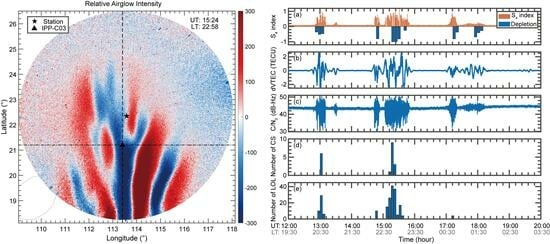
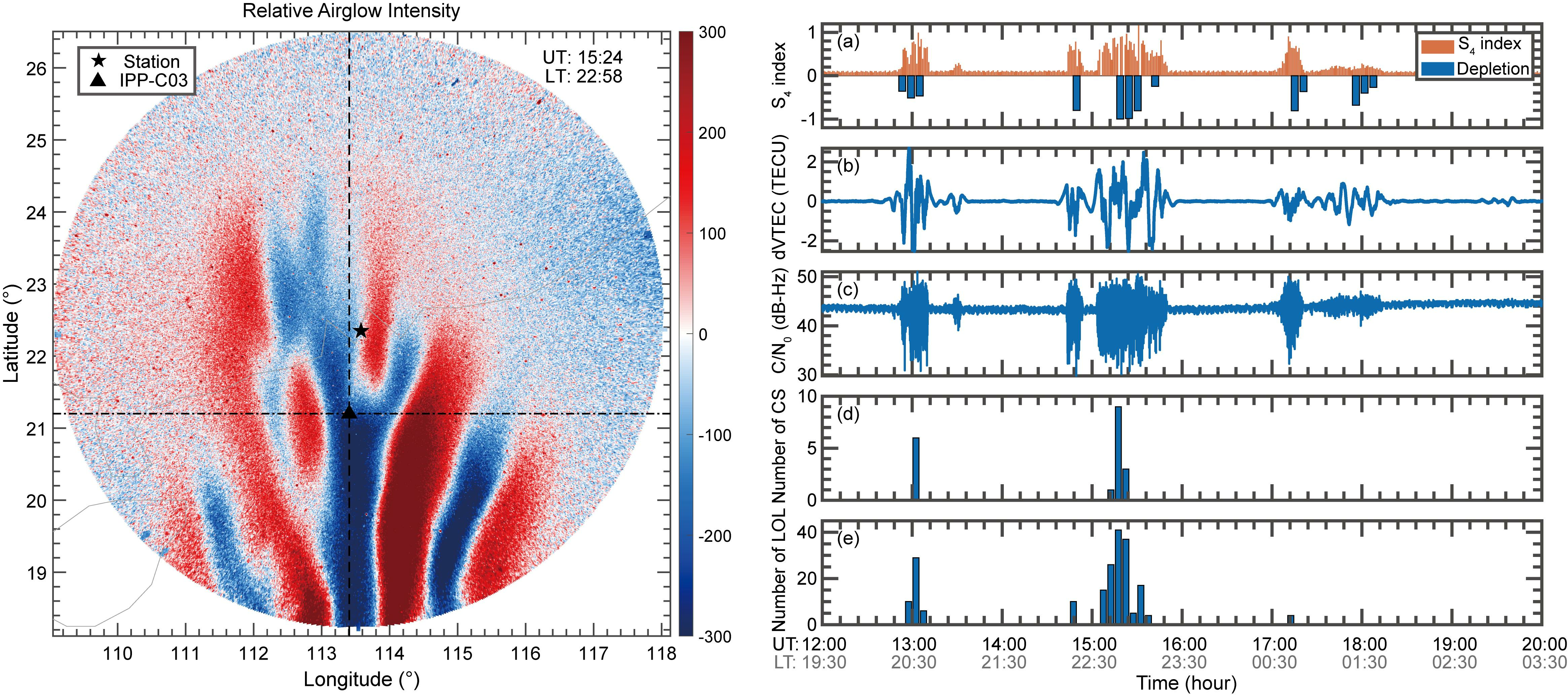
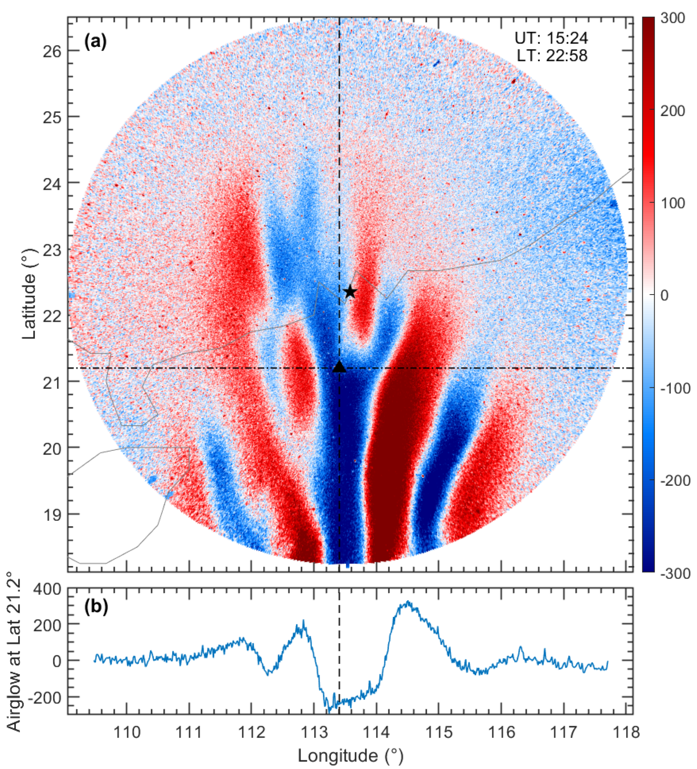
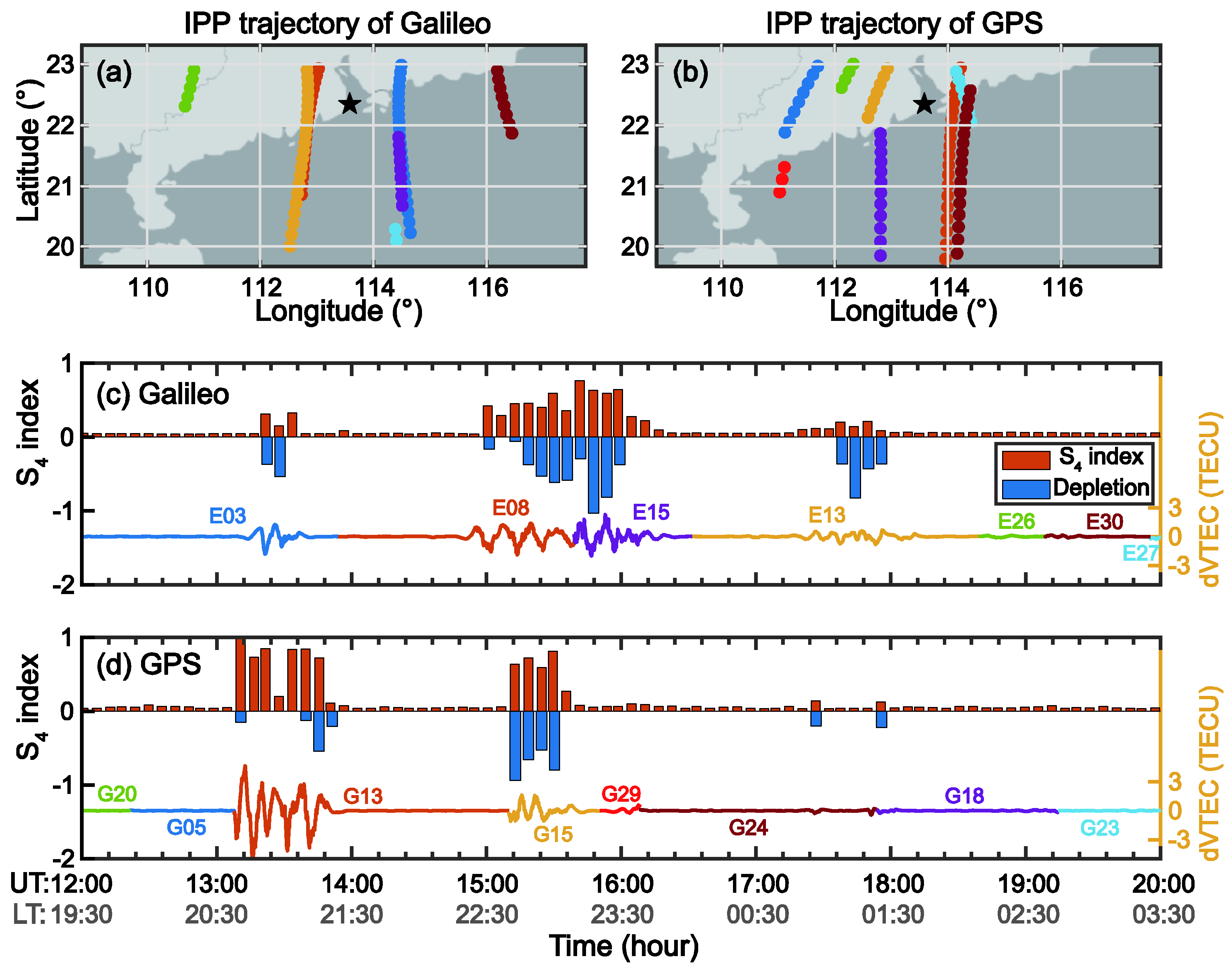
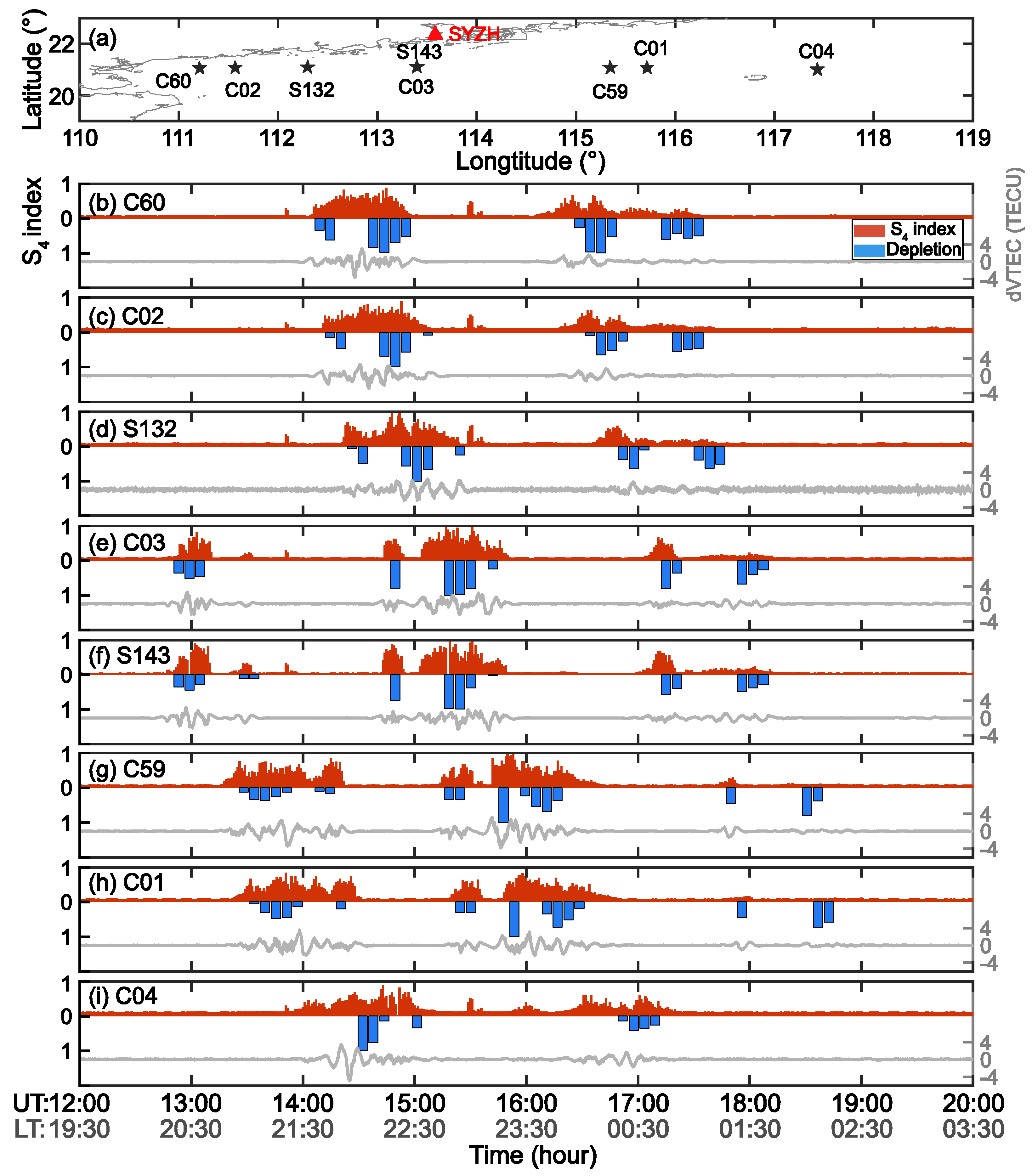
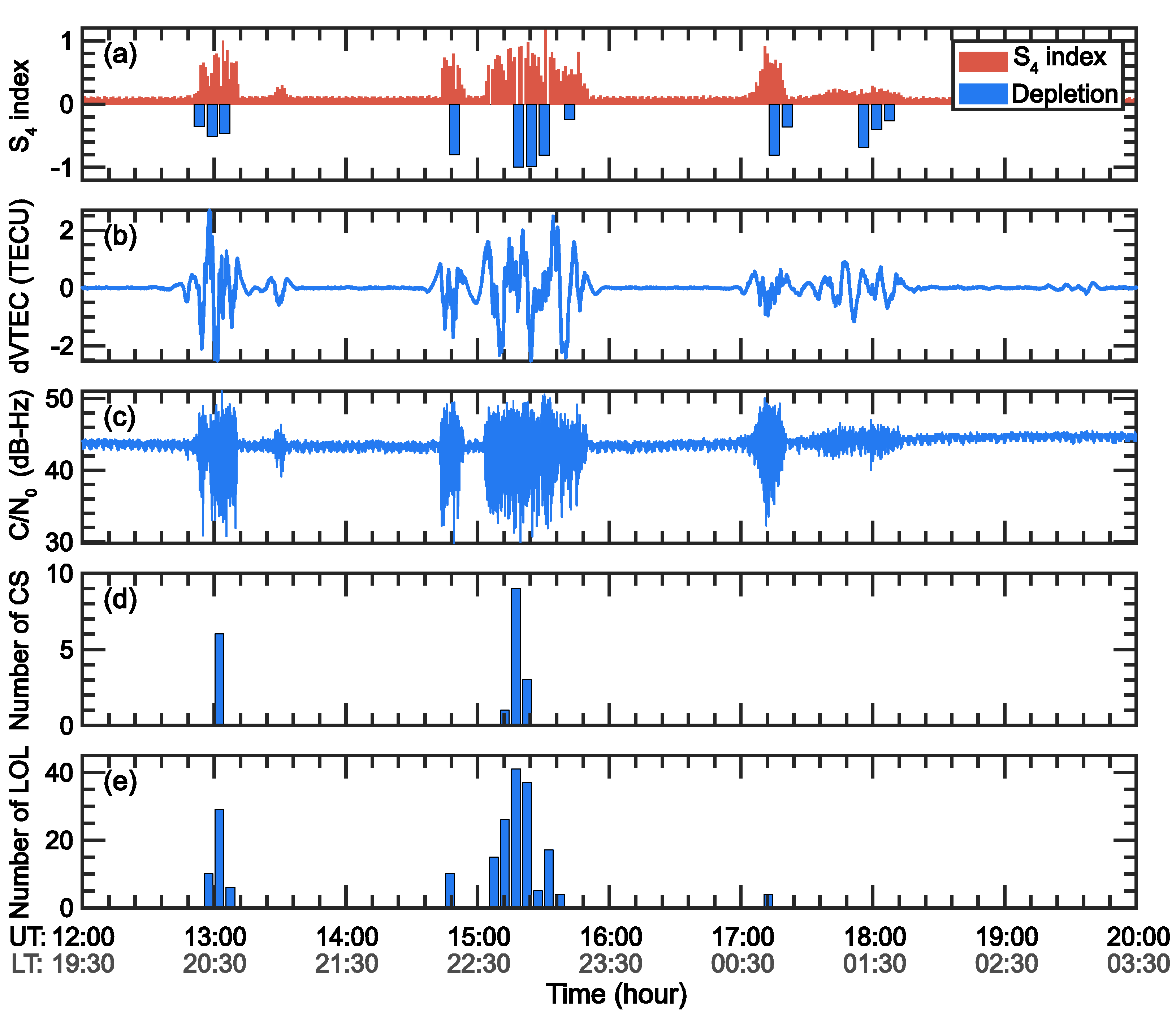
The joint airglow-GNSS observations reveal that the center part of the airglow depletion often corresponds to stronger GNSS scintillation, while the edge part of the bubble, which is considered to have the largest density gradient, corresponds to relatively smaller scintillation instead. The sharp fluctuations in dVTEC also correspond to the center of the airglow depletion.
(2)
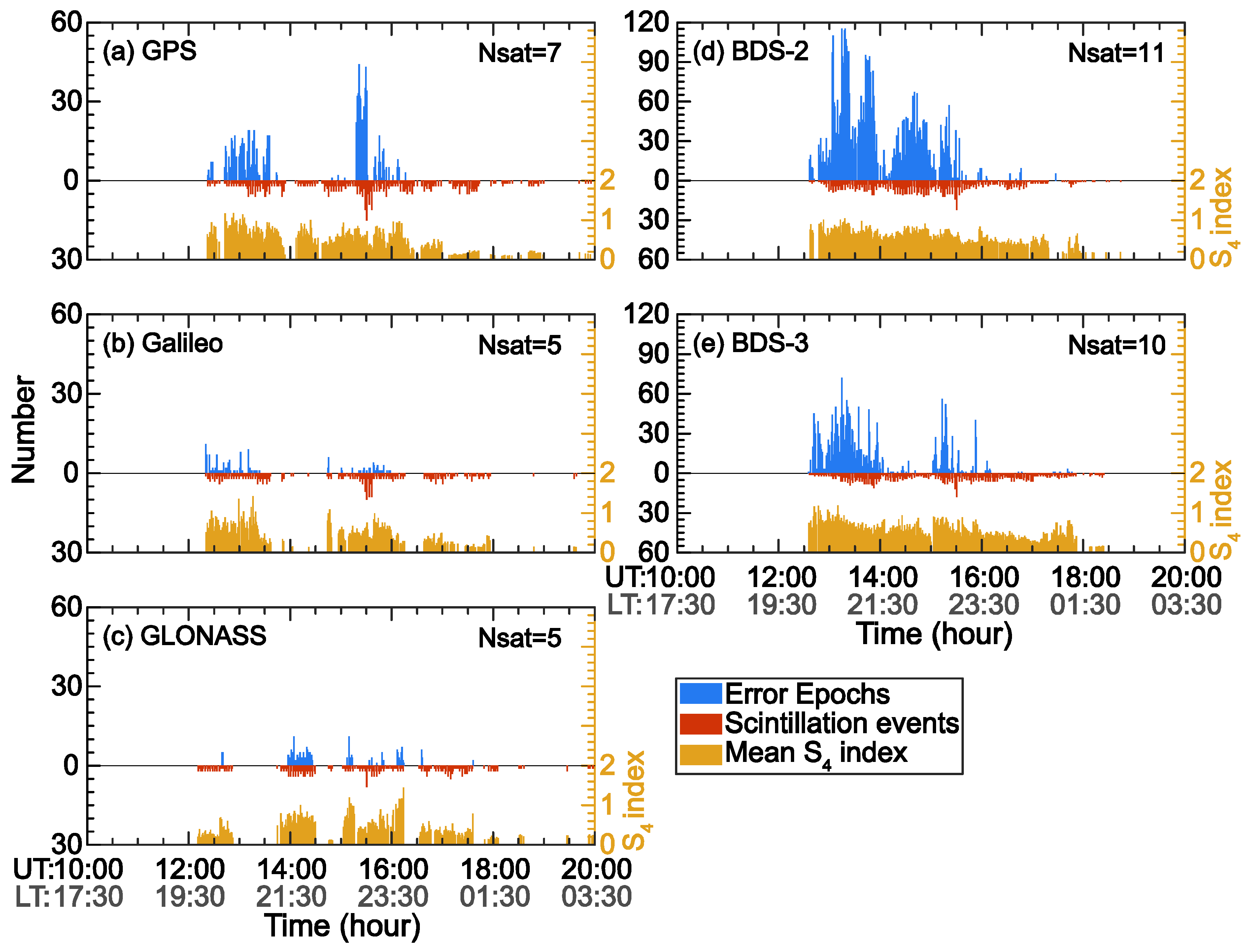
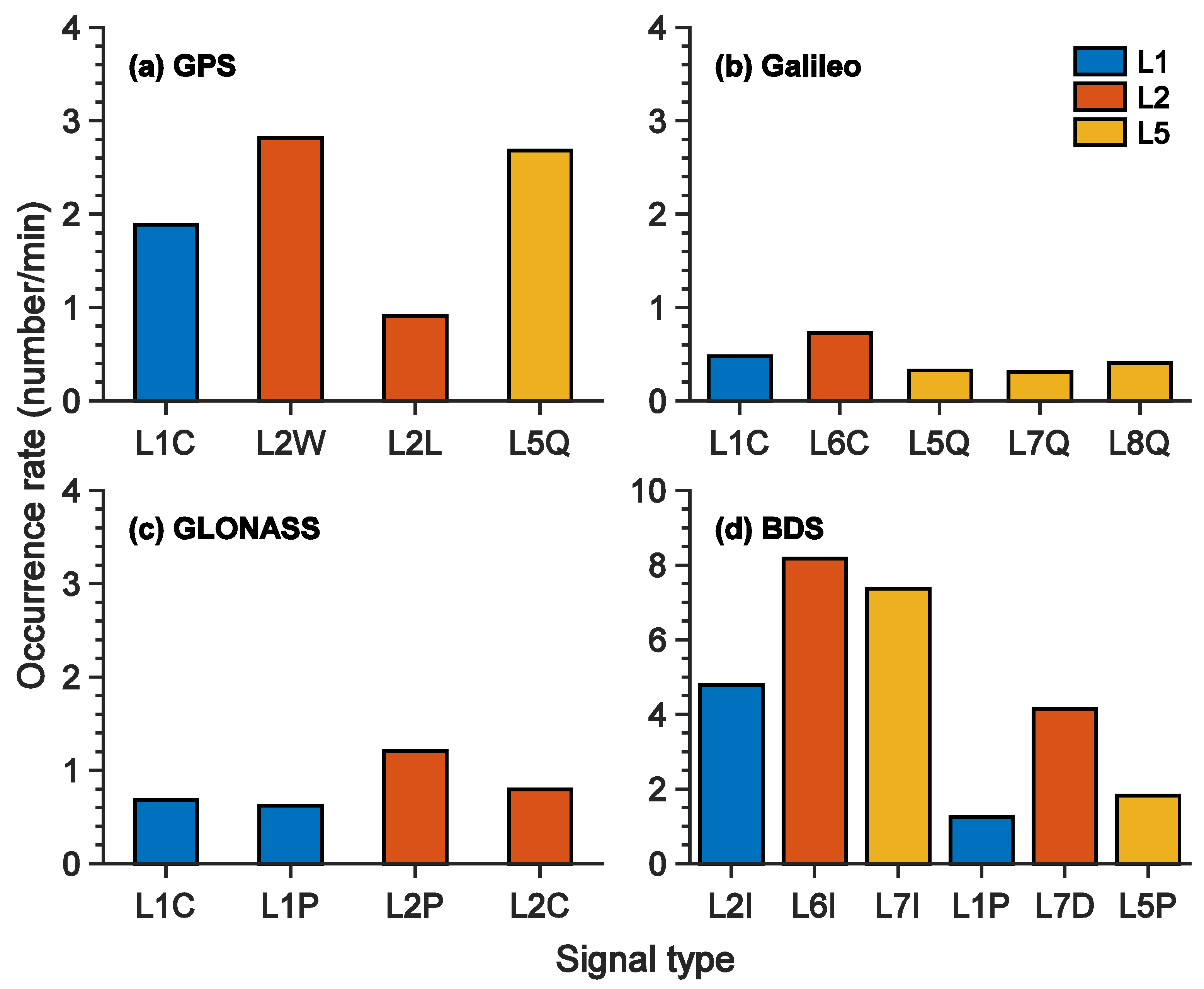
EPBs have significant impacts on GNSS signals, including signal strength degradation, loss of lock, and cycle slip, and these impacts are dependent on signal modulation for different GNSS constellations. The overall stability of the L1 band is better than that of the L2 and L5 bands, and signal tracking stability of Galileo is better than that of the others. For frequency selection in dual-frequency positioning, L1C and L2L for GPS, L1C and L5Q for Galileo, L1P and L2C for GLONASS, and L1P and L5P for BDS exhibit great signal tracking stability and could be better combinations during EPB events.
(3)
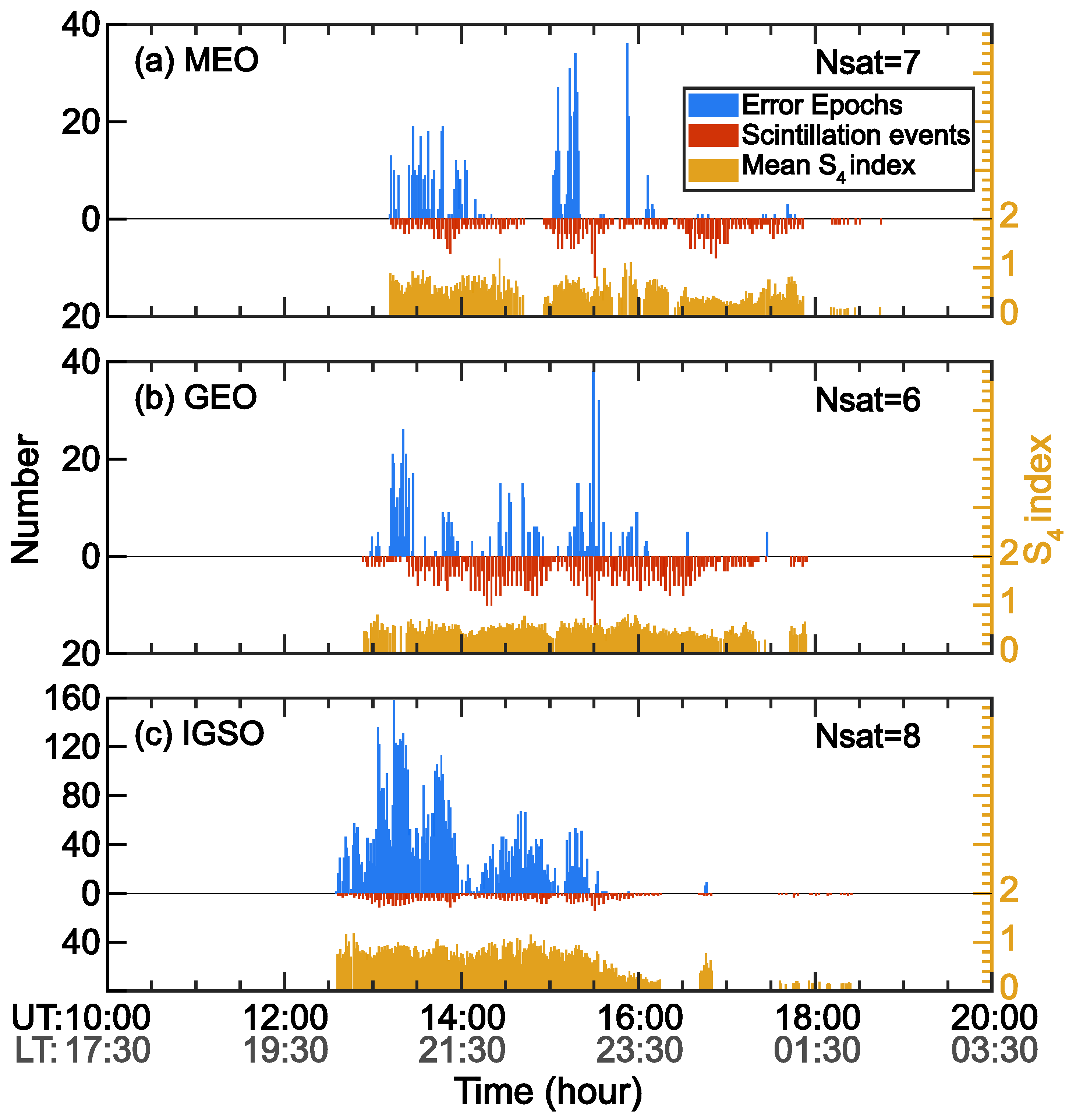
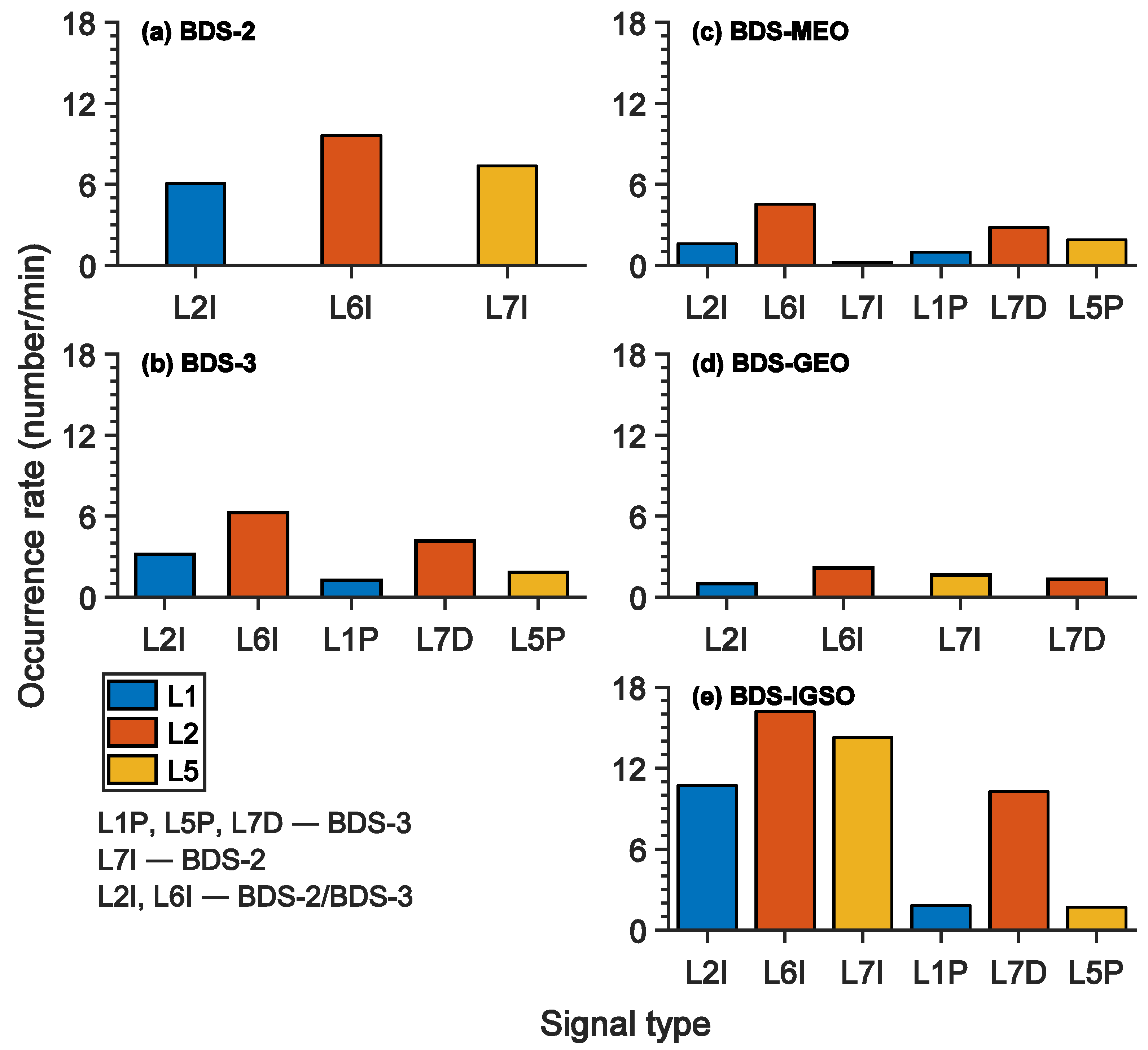
The BDS signals are further assessed according to different generations and satellite orbits. The signal tracking of BDS-3 is more stable than that of BDS-2. The performance of the IGSO satellites in BDS is far worse than that of the MEO and GEO satellites, which is likely related to the special signal path trajectory of the IGSO satellite.

Author Contributions

Conceptualization, H.H., J.Z., Y.H. and X.W.; methodology, J.Z., N.W. and X.W.; software, H.H., J.C., X.S., K.W. and Q.L.; validation, J.Z., Y.H., N.W., X.W. and F.H.; formal analysis, H.H., Y.T., Z.O. and W.D.; investigation, J.Z., Y.H., and N.W.; resources, H.H., J.Z., Y.H., and X.W.; data curation, J.Z., Q.L., F.H. and X.S.; writing—original draft preparation, H.H. and J.Z.; writing—review and editing, J.Z., Y.H., X.W. and F.H.; visualization, H.H., J.Z. and X.S.; supervision, H.H. and J.Z.; project administration, J.Z. and Y.H.; funding acquisition, J.Z. and Y.H. All authors have read and agreed to the published version of the manuscript.

Funding

This work was supported by the National Natural Science Foundation of China (42374181, 42374186, 42274195, 42004136, 42104169, 42104147, 41804150), the Project of Stable Support for Youth Team in Basic Research Field, CAS (YSBR-018), Guangdong Basic and Applied Basic Research Foundation (2021A1515011216, 2022A1515011580, 2020A1515110242), Joint Open Fund of Mengcheng National Geophysical Observatory (MENGO-202217), the USTC Research Funds of the Double First-Class Initiative (YD2080002013), the Opening Funding of Chinese Academy of Sciences dedicated for the Chinese Meridian Project.

Data Availability Statement

The GNSS and airglow data used and/or analyzed during the current study are openly available in https://zenodo.org/records/10960624 (doi: 10.5281/zenodo.10960623).

Acknowledgments

We thank NASA/Goddard Space Flight Center for providing the F107 index.

Conflicts of Interest

The authors declare no conflicts of interest.

References

  1. Kintner, P.M.; Ledvina, B.M.; de Paula, E.R. GPS and ionospheric scintillations. Space Weather 2007, 5, S09003. [Google Scholar] [CrossRef]
  2. Wernik, A.W.; Secan, J.A.; Fremouw, E.J. Ionospheric irregularities and scintillation. Adv. Space Res. 2003, 31, 971–981. [Google Scholar] [CrossRef]
  3. Jacobsen, K.S.; Andalsvik, Y.L. Overview of the 2015 St. Patrick’s day storm and its consequences for RTK and PPP positioning in Norway. J. Space Weather Space Clim. 2016, 6, A9. [Google Scholar] [CrossRef]
  4. Moreno, B.; Radicella, S.; de Lacy, M.C.; Herraiz, M.; Rodriguez-Caderot, G. On the effects of the ionospheric disturbances on precise point positioning at equatorial latitudes. GPS Solut. 2011, 15, 381–390. [Google Scholar] [CrossRef]
  5. Yousuf, M.; Dashora, N.; Sridhar, M.; Dutta, G. Long-term impact of ionospheric scintillations on kinematic precise point positioning: Seasonal and solar activity dependence over Indian low latitudes. GPS Solut. 2023, 27, 40. [Google Scholar] [CrossRef]
  6. Li, W.; Song, S.; Zhou, W.; Cheng, N.; Yu, C. Investigating the Impacts of Ionospheric Irregularities on Precise Point Positioning over China and Its Mechanism. Space Weather 2022, 20, e2022SW003236. [Google Scholar] [CrossRef]
  7. Sultan, P.J. Linear theory and modeling of the Rayleigh-Taylor instability leading to the occurrence of equatorial spread F. J. Geophys. Res. Space Phys. 1996, 101, 26875–26891. [Google Scholar] [CrossRef]
  8. Fejer, B.G.; Scherliess, L.; de Paula, E.R. Effects of the vertical plasma drift velocity on the generation and evolution of equatorial spread F. J. Geophys. Res. Space Phys. 1999, 104, 19859–19869. [Google Scholar] [CrossRef]
  9. Carter, B.A.; Yizengaw, E.; Retterer, J.M.; Francis, M.; Terkildsen, M.; Marshall, R.; Norman, R.; Zhang, K. An analysis of the quiet time day-to-day variability in the formation of postsunset equatorial plasma bubbles in the Southeast Asian region. J. Geophys. Res. Space Phys. 2014, 119, 3206–3223. [Google Scholar] [CrossRef]
  10. Currie, J.L.; Carter, B.A.; Retterer, J.; Dao, T.; Pradipta, R.; Caton, R.; Groves, K.; Otsuka, Y.; Yokoyama, T.; Hozumi, K.; et al. On the Generation of an Unseasonal EPB over South East Asia. J. Geophys. Res. Space Phys. 2021, 126, e2020JA028724. [Google Scholar] [CrossRef]
  11. Kelley, M.C. The Earth’s Ionosphere Plasma Physics and Electrodynamics; Academic Press: San Diego, CA, USA, 2009; Volume 96. [Google Scholar]
  12. Ma, G.; Maruyama, T. A super bubble detected by dense GPS network at east Asian longitudes. Geophys. Res. Lett. 2006, 33, L21103. [Google Scholar] [CrossRef]
  13. Unnikrishnan, K.; Sreekumar, H.; Choudhary, R.K.; Ashna, V.M.; Ambili, K.M.; Shreedevi, P.R.; Rao, P.B. A study on the evolution of plasma bubbles using the single station-multisatellite and multistation-single satellite techniques. J. Geophys. Res. Space Phys. 2017, 122, 3678–3688. [Google Scholar] [CrossRef]
  14. Seo, J.; Walter, T.; Enge, P. Availability Impact on GPS Aviation due to Strong Ionospheric Scintillation. IEEE Trans. Aerosp. Electron Syst. 2011, 47, 1963–1973. [Google Scholar] [CrossRef]
  15. Kil, H.; Kintner, P.M.; de Paula, E.R.; Kantor, I.J. Latitudinal variations of scintillation activity and zonal plasma drifts in South America. Radio Sci. 2002, 37, 1006. [Google Scholar] [CrossRef]
  16. Klobuchar, J.A.; Anderson, D.N.; Doherty, P.H. Model Studies of the Latitudinal Extent of the Equatorial Anomaly during Equinoctial Conditions. Radio Sci. 1991, 26, 1025–1047. [Google Scholar] [CrossRef]
  17. Basu, S.; Kudeki, E.; Basu, S.; Valladares, C.E.; Weber, E.J.; Zengingonul, H.P.; Bhattacharyya, S.; Sheehan, R.; Meriwether, J.W.; Biondi, M.A.; et al. Scintillations, plasma drifts, and neutral winds in the equatorial ionosphere after sunset. J. Geophys. Res. Space Phys. 1996, 101, 26795–26809. [Google Scholar] [CrossRef]
  18. Basu, S.; MacKenzie, E.; Basu, S. Ionospheric constraints on VHF/UHF communications links during solar maximum and minimum periods. Radio Sci. 1988, 23, 363–378. [Google Scholar] [CrossRef]
  19. de Paula, E.R.; Rodrigues, F.S.; Iyer, K.N.; Kantor, I.J.; Abdu, M.A.; Kintner, P.M.; Ledvina, B.M.; Kil, H. Equatorial anomaly effects on GPS scintillations in brazil. Adv. Space Res. 2003, 31, 749–754. [Google Scholar] [CrossRef]
  20. Muella, M.T.A.H.; Duarte-Silva, M.H.; Moraes, A.O.; de Paula, E.R.; de Rezende, L.F.C.; Alfonsi, L.; Affonso, B.J. Climatology and modeling of ionospheric scintillations and irregularity zonal drifts at the equatorial anomaly crest region. Ann. Geophys. 2017, 35, 1201–1218. [Google Scholar] [CrossRef]
  21. Damaceno, J.G.; Bolmgren, K.; Bruno, J.; De Franceschi, G.; Mitchell, C.; Cafaro, M. GPS loss of lock statistics over Brazil during the 24th solar cycle. Adv. Space Res. 2020, 66, 219–225. [Google Scholar] [CrossRef]
  22. Srinivasu, V.K.D.; Dashora, N.; Prasad, D.S.V.V.D.; Niranjan, K. Loss of lock on GNSS signals and its association with ionospheric irregularities observed over Indian low latitudes. GPS Solut. 2022, 26, 34. [Google Scholar] [CrossRef]
  23. Mulugeta, S.; Kassa, T. Investigation of GPS Loss of Lock occurrence and Its characteristics over Ethiopia using Geodetic GPS receivers of the IGS network. Adv. Space Res. 2022, 69, 939–950. [Google Scholar] [CrossRef]
  24. Zhang, D.; Feng, M.; Xiao, Z.; Hao, Y.; Shi, L.; Yang, G.; Suo, Y. The seasonal dependence of cycle slip occurrence of GPS data over China low latitude region. Sci. China Ser. E Technol. Sci. 2007, 50, 422–429. [Google Scholar] [CrossRef]
  25. Zhang, D.H.; Cai, L.; Hao, Y.Q.; Xiao, Z.; Shi, L.Q.; Yang, G.L.; Suo, Y.C. Solar cycle variation of the GPS cycle slip occurrence in China low-latitude region. Space Weather 2010, 8, S10D10. [Google Scholar] [CrossRef]
  26. Srinivasu, V.K.D.; Dashora, N.; Prasad, D.S.V.V.D.; Niranjan, K.; Gopi Krishna, S. On the occurrence and strength of multi-frequency multi-GNSS Ionospheric Scintillations in Indian sector during declining phase of solar cycle 24. Adv. Space Res. 2018, 61, 1761–1775. [Google Scholar] [CrossRef]
  27. Biswas, T.; Ghosh, S.; Paul, A.; Sarkar, S. Interfrequency Performance Characterizations of GPS during Signal Outages from an Anomaly Crest Location. Space Weather 2019, 17, 803–815. [Google Scholar] [CrossRef]
  28. Salles, L.A.; Vani, B.C.; Moraes, A.; Costa, E.; de Paula, E.R. Investigating Ionospheric Scintillation Effects on Multifrequency GPS Signals. Surv. Geophys. 2021, 42, 999–1025. [Google Scholar] [CrossRef]
  29. Salles, L.A.; Moraes, A.; Vani, B.; Sousasantos, J.; Affonso, B.J.; Monico, J.F.G. A deep fading assessment of the modernized L2C and L5 signals for low-latitude regions. GPS Solut. 2021, 25, 122. [Google Scholar] [CrossRef]
  30. Song, K.; Meziane, K.; Kashcheyev, A.; Jayachandran, P.T. Multifrequency Observation of High Latitude Scintillation: A Comparison With the Phase Screen Model. IEEE Trans. Geosci. Remote Sens. 2022, 60, 5801209. [Google Scholar] [CrossRef]
  31. Liu, H.; Ren, X.; Zhang, X.; Mei, D.; Yang, P. Investigating the Effects of Ionospheric Scintillation on Multi-Frequency BDS-2/BDS-3 Signals at Low Latitudes. Space Weather 2023, 21, e2022SW003362. [Google Scholar] [CrossRef]
  32. Sleewaegen, J.-M.; Wilde, W.D.; Hollreiser, M. Galileo AltBOC Receiver. In Proceedings of the ION GNSS 2004, Rotterdam, The Netherlands, 16–19 May 2004. [Google Scholar]
  33. Padokhin, A.M.; Mylnikova, A.A.; Yasyukevich, Y.V.; Morozov, Y.V.; Kurbatov, G.A.; Vesnin, A.M. Galileo E5 AltBOC Signals: Application for Single-Frequency Total Electron Content Estimations. Remote Sens. 2021, 13, 3973. [Google Scholar] [CrossRef]
  34. de Oliveira Moraes, A.; Muella, M.T.A.H.; de Paula, E.R.; de Oliveira, C.B.A.; Terra, W.P.; Perrella, W.J.; Meibach-Rosa, P.R.P. Statistical evaluation of GLONASS amplitude scintillation over low latitudes in the Brazilian territory. Adv. Space Res. 2018, 61, 1776–1789. [Google Scholar] [CrossRef]
  35. Goswami, S.; Paul, A.; Haldar, S. Study of Relative Performance of Different Navigational Satellite Constellations under Adverse Ionospheric Conditions. Space Weather 2018, 16, 667–675. [Google Scholar] [CrossRef]
  36. Blewitt, G. An automatic editing algorithm for GPS data. Geophys. Res. Lett. 1990, 17, 199–202. [Google Scholar] [CrossRef]
  37. Keshin, M. A new algorithm for single receiver DCB estimation using IGS TEC maps. GPS Solut. 2012, 16, 283–292. [Google Scholar] [CrossRef]
  38. Savitzky, A.; Golay, M.J.E. Smoothing and Differentiation of Data by Simplified Least Squares Procedures. Anal. Chem. 1964, 36, 1A–121A. [Google Scholar] [CrossRef]
  39. Conker, R.S.; El-Arini, M.B.; Hegarty, C.J.; Hsiao, T. Modeling the effects of ionospheric scintillation on GPS/Satellite-Based Augmentation System availability. Radio Sci. 2003, 38, 1001. [Google Scholar] [CrossRef]
  40. Dousa, P.V.J. G-Nut Anubis Open Source Tool for Multi-GNSS Data Monitoring with a Multipath Detection for New Signals, Frequencies and Constellations; Springer: Berlin/Heidelberg, Germany, 2016; Volume 143, pp. 775–782. [Google Scholar]
  41. Zhao, Q.; Sun, B.; Dai, Z.; Hu, Z.; Shi, C.; Liu, J. Real-time detection and repair of cycle slips in triple-frequency GNSS measurements. GPS Solut. 2014, 19, 381–391. [Google Scholar] [CrossRef]
  42. Otsuka, Y.; Shiokawa, K.; Ogawa, T.; Wilkinson, P. Geomagnetic conjugate observations of equatorial airglow depletions. Geophys. Res. Lett. 2002, 29, 1753. [Google Scholar] [CrossRef]
  43. Li, Z.; Zhong, J.; Hao, Y.; Zhang, M.; Niu, J.; Wan, X.; Huang, F.; Han, H.; Song, X.; Chen, J. Assessment of the orbital variations of GNSS GEO and IGSO satellites for monitoring ionospheric TEC. GPS Solut. 2023, 27, 62. [Google Scholar] [CrossRef]
  44. Demyanov, V.V.; Yasyukevich, Y.V.; Ishin, A.B.; Astafyeva, E.I. Ionospheric super-bubble effects on the GPS positioning relative to the orientation of signal path and geomagnetic field direction. GPS Solut. 2011, 16, 181–189. [Google Scholar] [CrossRef]
  45. Carrano, C.S.; Rino, C.L. A theory of scintillation for two-component power law irregularity spectra: Overview and numerical results. Radio Sci. 2016, 51, 789–813. [Google Scholar] [CrossRef]
  46. Bhattacharyya, A.; Kakad, B.; Gurram, P.; Sripathi, S.; Sunda, S. Development of intermediate-scale structure at different altitudes within an equatorial plasma bubble: Implications for L-band scintillations. J. Geophys. Res. Space Phys. 2017, 122, 1015–1030. [Google Scholar] [CrossRef]
  47. de O. Moraes, A.; Vani, B.C.; Costa, E.; Sousasantos, J.; Abdu, M.A.; Rodrigues, F.; Gladek, Y.C.; de Oliveira, C.B.A.; Monico, J.F.G. Ionospheric Scintillation Fading Coefficients for the GPS L1, L2, and L5 Frequencies. Radio Sci. 2018, 53, 1165–1174. [Google Scholar] [CrossRef]
  48. Luo, X.; Liu, Z.; Lou, Y.; Gu, S.; Chen, B. A study of multi-GNSS ionospheric scintillation and cycle-slip over Hong Kong region for moderate solar flux conditions. Adv. Space Res. 2017, 60, 1039–1053. [Google Scholar] [CrossRef]
  49. Anderson, P.C.; Straus, P.R. Magnetic field orientation control of GPS occultation observations of equatorial scintillation. Geophys. Res. Lett. 2005, 32, L21107. [Google Scholar] [CrossRef]
Figure 1. An example of a post-processed airglow image at 15:24 UT on 3 April 2022. (a) Geographical distribution of relative airglow values with pseudocolor. The black star represents the location of the ground station, and the black triangle represents the ionospheric pierce point (IPP) location of BDS GEO satellite C03 at 300 km. The dashed and dash-dot lines mark the longitude and latitude of the IPP, respectively. (b) Airglow values at a fixed latitude of 21.2° extracted from panel (a). The black dashed line indicates the airglow value extracted at the fixed IPP.
Remotesensing 16 01358 g001
Figure 2. Comparison of the S4 index (Galileo: L1C, GPS: L1C), airglow depletion, and deviation VTEC (Galileo: L1C-L5Q, GPS: L1C-L2W) for (a,c) Galileo and (b,d) GPS during 12–20 UT on 3 April 2022. The signal path with the highest elevation is selected among all the satellites at a certain epoch. (a,b) Distributions of the selected ionospheric pierce points (IPPs, color dots) at an effective height of 300 km. The selected area is at 19°–23°N, which is covered by the airglow image. The black stars represent the location of the GNSS receiver and airglow imager at Zhuhai, China. (c,d) Variations of the S4 index (orange bar), airglow depletion (blue bar), and deviation VTEC (colored line) as a function of UT (LT ≈ UT + 7.5). The airglow values are the post-processed airglow values divided by a constant value (it is 200 in this work). The specific PRNs are also marked in the panels, and the colors used for specific PRNs are the same in panels (a,c).
Remotesensing 16 01358 g002
Figure 3. Comparison of the S4 index (BDS: L2I, SBAS: L1C), airglow depletion, and deviation VTEC (BDS: L2I-L6I, SBAS: L1C-L5I) for eight GEO satellites during 12–20 UT on 3 April 2022. (a) Geographical distribution of ground-based station (red triangle) and IPPs (black pentagrams) for eight GEO satellites. From top to bottom (bi) are eight GEO satellites distributed from west to east.
Remotesensing 16 01358 g003
Figure 4. Variations of signal quality parameters for L6I (1268.52 MHz) observations from the BDS-C03 GEO satellite during 12–20 UT on 3 April 2022. From top to bottom are the variations of (a) the S4 index (L6I) and airglow depletion, (b) the deviation VTEC (L2I-L6I), (c) the signal-to-noise ratio (C/N0, S6I), (d) the number of cycle slips, and (e) the number of losses of lock as a function of UT.
Remotesensing 16 01358 g004
Figure 5. Comparison of the number of error epochs (cycle slip or loss of phase observation, blue bar), number of scintillation events (S4 > 1.5* averaged S4, orange bar), and corresponding mean S4 intensity (yellow bar) at L1 frequency (GPS L1C, Galileo L1C, GLONASS L1C: 1575.42 MHz, and BDS-2 and BDS-3 L2I: 1561.098 MHz) band for different constellations. For better comparison with the S4 index, the error epochs are divided into 1 min time bins. The constellation is marked in the upper left corner of each subpanel, and the upper right corner indicates the average number of satellites observed at each epoch.
Remotesensing 16 01358 g005
Figure 6. Comparison of the number of error epochs, number of scintillation events, and corresponding mean S4 intensity for three orbits (MEO, GEO, IGSO) of the BDS at L1 frequency (L2I, 1561.098 MHz). This figure is similar to Figure 5.
Remotesensing 16 01358 g006
Figure 7. Occurrence rate of error epochs for (a) GPS, (b) Galileo, (c) GLONASS, and (d) BDS during 12–20 UT on 3 April 2022. The color of the bar indicates the frequency band and the signal types are marked in x-label. When the S4 index exceeds the threshold, the signal is considered to have passed through the EPB at this time. The occurrence rate is defined as the total epoch of cycle slips and loss of phase observations divided by the total epoch in which the signal passes through the EPB in 1 min.
Remotesensing 16 01358 g007
Figure 8. Occurrence rate of error epochs for BDS-2 and BDS-3 and for different orbit types (MEO, GEO, IGSO). This figure is similar to Figure 7.
Remotesensing 16 01358 g008
Table 1. List of the BDS-2 satellites used in this study. The longitudes of the sub-satellite points for GEO satellites and the longitudes of the intersection of sub-satellite trajectories for IGSO satellites are shown in the third column.
PRNSatellite NameLongitude (°E)Lauch Date
C04BDS-2 GEO416031 October 2010
C05BDS-2 GEO55924 February 2012
C02BDS-2 GEO68425 October 2012
C03BDS-2 GEO7110.512 June 2016
C01BDS-2 GEO8144.517 May 2019
C06BDS-2 IGSO1105.531 July 2010
C07BDS-2 IGSO2106.517 December 2010
C08BDS-2 IGSO31059 April 2011
C09BDS-2 IGSO495.926 July 2011
C10BDS-2 IGSO5941 December 2011
C13BDS-2 IGSO69611 October 2016
C16BDS-2 IGSO7113.59 July 2018
C11BDS-2 MEO3-29 April 2012
C12BDS-2 MEO4-29 April 2012
C14BDS-2 MEO6-18 September 2012
Table 2. List of the BDS-3 satellites used in this study. The longitudes of the sub-satellite points for GEO satellites and the longitudes of the intersection of sub-satellite trajectories for IGSO satellites are shown in the third column.
PRNSatellite NameLongitude (°E)Lauch Date
C59BDS-3 GEO11401 November 2018
C60BDS-3 GEO2809 March 2020
C38BDS-3 IGSO111920 April 2019
C39BDS-3 IGSO2118.524 June 2019
C40BDS-3 IGSO3119.55 November 2019
C19BDS-3 MEO1-5 November 2017
C28BDS-3 MEO8-11 January 2018
C21BDS-3 MEO3-12 February 2018
C22BDS-3 MEO4-12 February 2018
C29BDS-3 MEO9-29 March 2018
C23BDS-3 MEO5-29 July 2018
C24BDS-3 MEO6-29 July 2018
C26BDS-3 MEO11-24 August 2018
C25BDS-3 MEO12-24 August 2018
C33BDS-3 MEO14-19 September 2018
C35BDS-3 MEO15-15 October 2018
C34BDS-3 MEO16-15 October 2018
C45BDS-3 MEO23-23 September 2019
C43BDS-3 MEO21-23 November 2019
C44BDS-3 MEO22-23 November 2019
C41 BDS-3 MEO19-16 December 2019
C42BDS-3 MEO20-16 December 2019
Disclaimer/Publisher’s Note: The statements, opinions and data contained in all publications are solely those of the individual author(s) and contributor(s) and not of MDPI and/or the editor(s). MDPI and/or the editor(s) disclaim responsibility for any injury to people or property resulting from any ideas, methods, instructions or products referred to in the content.

