Abstract
The deep seabed is composed of heterogeneous ecosystems, containing diverse habitats for marine life. Consequently, understanding the geological and ecological characteristics of the seabed’s features is a key step for many applications. The majority of approaches commonly use optical and acoustic sensors to address these tasks; however, each sensor has limitations associated with the underwater environment. This paper presents a survey of the main techniques and trends related to seabed characterization, highlighting approaches in three tasks: classification, detection, and segmentation. The bibliography is categorized into four approaches: statistics-based, classical machine learning, deep learning, and object-based image analysis. The differences between the techniques are presented, and the main challenges for deep sea research and potential directions of study are outlined.
1. Introduction
The deep ocean is one of the largest and least explored ecosystems on Earth [,]. It starts around 200 m in depth and reaches approximately 11,000 m. In addition, the deep sea contains heterogeneous ecosystems featuring vast marine flora and fauna. Therefore, comprehending the geological and ecological characteristics of the seabed is a fundamental process for several applications. The conventional methods of seabed sediment classification use sampler types, such as towed samplers, bottom samplers, and seafloor photography []. Nevertheless, these techniques have some drawbacks, including the requirement for heavy equipment, time consumption, and intensive manual labor. Consequently, applying remote sensing technology to characterize seabeds has received substantial attention within the academic community [].
Underwater sensing is the acquisition of data from underwater environments. With the rapid development of technology, a broad set of sensors have been used to perform various tasks in marine research [,]. The most commonly used sensors are based on optics and acoustics, each designed for specific applications and scenarios, such as seafloor mapping [], object inspection [], navigation [], and many others. Considering acoustics sensors, there are Single-beam Echosounders (SBESs), Multibeam Echosounders (MBESs), side-scan Sound Navigation and Ranging (SONAR), and sub-bottom profilers. For optical sensing, typical sensors are underwater cameras, three-dimensional (3D) underwater structured light sensors, and hyperspectral sensors. In this context of deep and potentially large areas of the sea, underwater vehicles are fundamental for carrying out such operational missions. Sensors are attached to these mobile robots, namely Autonomous Underwater Vehicles (AUVs) and Remotely Operated Vehicles (ROVs), enabling the collection and processing of a large amount of data at depths unreachable by humans, thus achieving real-time data processing.
Recently, the deep sea has been the focus of significant research efforts due to the presence of mineral resources, including polymetallic nodules, cobalt-rich crusts, and massive sulfides, thus presenting great importance to deep sea mining [,,,,]. Specifically, polymetallic nodules are small gravel-sized encrustations with spheroidal or ellipsoidal shapes that are found on the deep seafloor, containing critical metals such as nickel, copper, cobalt, manganese, and rare earth elements. These nodules have attracted interest due to their potential as a source of raw materials for various industries [].
Conversely, the deep sea is a unique and fragile environment, and the effects of mining on marine life have yet to be fully explored and understood []. Hazard assessment studies, such as [,], indicate the environmental impact of current mining technologies. The collector mechanisms are typically seabed sweeping [] or pump systems []. Furthermore, polymetallic nodules are also part of the ocean ecosystem; consequently, their exploration can harm the habitat. For instance, a large quantity of nodules is required for exploration to have an economic benefit. Given that the nodules are generally located at great depths, underwater vehicles are essential for the perception and awareness of nodules. Thus, deep sea mining is a complex and challenging topic, and an improved seafloor characterization can lead to better resource management and nodule assessment, reducing environmental impact.
Another important application that can be enhanced with improved seabed classification is deep coral reef monitoring. Coral reefs are extremely related to the oceans’ health, harboring a diverse variety of species []. However, due to human impacts and climate change, those coral species are endangered []. For instance, recent studies have indicated that some coral species are hastily decreasing, being subjected to bleaching and the degradation of reef structures [,]. Hence, being able to monitor these species and perform constant assessments of their status becomes fundamental in order to achieve sustainable development.
Characterizing the seabed is a major goal in several robotic tasks. There are considerable surveys regarding different techniques, especially deep learning (DL) and machine learning (ML). However, these surveys only focus on one modality, such as acoustic [,], optical [,], or hyperspectral sensors []. Furthermore, the previous research generally covers only one type of method, machine learning, for instance. Hence, a survey that covers a comprehensive study of multiple sensing methods and technologies is still needed. The objective of this research was to identify a variety of seabed characterization techniques, considering three levels of detail: classification, detection, and segmentation (as depicted in Figure 1). The study also focused on identifying the primary technologies for data collection, rather than solely focusing on one, resulting in a more broad study.
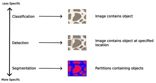
Figure 1.
Three levels of tasks for seabed characterization.
Following this motivation, the paper outline is as follows. In Section 2, we define seafloor characterization and the environmental challenges. Then, Section 3 presents common technologies used for seafloor characterization. Section 4 focuses on the related work, identifying the key approaches for seabed classification and mapping. Next, Section 5 provides a comparative analysis of the surveyed papers, presenting the main advantages and drawbacks and suggesting potential research directions. Finally, the main conclusions are presented in Section 6.
2. Seafloor Characterization
Seafloor characterization can be defined as describing the topographic, physical, geological, and biological properties of the seabed. To achieve this, multiple sensors and sensing methodologies are used to obtain data for processing. Additionally, the knowledge of seabed characteristics is important for several applications in the field of marine robotics, such as geological surveys, underwater inspections, habitat mapping, object detection, and others.
Underwater Environment Challenges
Although significant advances have occurred in sensor technology for underwater scenarios to overcome technical challenges such as high pressure, power consumption, and data processing and transmission, the underwater environment still presents itself as a challenging scenario for underwater robotics and sensing [,]. Figure 1 illustrates some issues in underwater images, and Figure 2 was obtained at the kaolin mine in Lee Moor, United Kingdom, during the VAMOS project []. Typical underwater computer vision systems face the following issues.
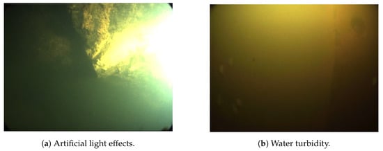
Figure 2.
Examples of underwater environment constraints.
- Lighting conditions: Light is absorbed by water across almost all wavelengths, although it typically attenuates blue and green wavelengths to a lesser extent. Furthermore, the degree of color change resulting from light attenuation varies based on several factors, including the wavelength of the light, the amount of dissolved organic compounds, the water’s salinity, and the concentration of phytoplankton [,]. Recently, there has been an increase in image-enhancement algorithms that can be categorized into three approaches: statistical [], physical [], and learning-based [,].
- Backscattering: The diffuse reflection of light rays can lead to image blurring and noise. Suspended particles cause light from ambient illumination sources to scatter towards the camera [].
- Image texture: Textures significantly help in the identification of given features of the image. However, in underwater imagery, textures may not be discernible, which makes it difficult to calculate relative displacement or accurately determine the scene depth [].
- Vignetting effect: This refers to a reduction in the brightness or saturation of an image towards its periphery, as compared to the center of the image, as observed in Figure 2 [].
- Nonexistence of ambient light: The unavailability of ambient light in the deep sea introduces additional problems related to the need to provide artificial lighting, such as uneven distributions, and sources of light generally close to the imaging sensors add difficulties in varying the incident angle [].
Similarly, acoustic sensors also present issues in underwater scenarios, such as the following.
- Noise: Underwater environments can be noisy due to currents, and other sources of interference, making it difficult for acoustic systems to accurately transmit and receive signals []. In general, noise is described as a Gaussian statistical distribution through a continuous power spectral density [].
- Signal attenuation: The two main factors that influence this property are the absorption and the spreading loss. Absorption refers to the process of signal attenuation due to the conversion of the acoustic energy to heat []. On the other hand, spreading loss refers to the decreasing of acoustic energy as the singla spreads through the medium [].
- Multi-path propagation: Reception of a single acoustic signal in multiple instances due to its transmission via multiple paths such as through refraction. For this reason, false positives can occur since the same signal is received at different instants [].
3. Underwater Sensing
3.1. Acoustic Ranging/Imaging Sensors
Standard sensors for geological survey applications, such as seafloor mapping and resource exploration, are based on SONAR data. They provided a non-invasive way to generate seafloor maps. The most common are the following:
- Single-beam Echosounder: SBES uses transducers, typically ceramic or piezoelectric crystals, to transmit and receive acoustic signals. The principle of operation of this sensor is to calculate the signal travel time, that is, the time difference between signal emission and reception. Knowing the propagation speed of sound c and the time of flight t, the distance d is calculated asThe main advantage of this sensor is that it is relatively easy to use and has a low cost compared with other sensors. On the other hand, the coverage area is small, generally between 2–12 degrees [], preventing it from obtaining broad coverage. Figure 3 illustrates the principle of operation.
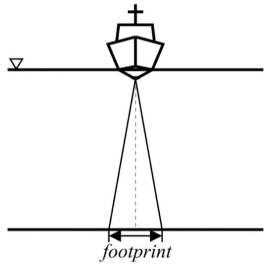
Figure 3.
Single-beam echosounder (Adapted from []).
- Multibeam echosounder: As the name implies, the principle of operation of MBES corresponds to multiple beams emitted simultaneously. Consisting of an array of transducers, this system emits multiple acoustic beams and captures the echoes reflected from the seabed, covering a wide swath of the seafloor. The subsequent processing of the received echoes results in the generation of detailed bathymetric maps. Conforming to [], the sensors can also be divided into narrow and wide systems. In narrow systems, there is a trade-off of obtaining high spatial resolution and a limited coverage area with each transmission. Figure 4 illustrates the sensor. The bathymetric data, or water depth, provided by echosounders depends on the range detection, which is surveyed in swaths. If the sensor position and orientation are, the beam angle is also known, and a point cloud can be generated. Consequently, the terrain model can be obtained from a point cloud [,]. For this reason, bathymetry data are essential to obtain seafloor topography and morphology information [,].
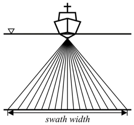 Figure 4. Multibeam echosounder (Adapted from []).
 - Side-scan sonar: A side-scan sonar has seabed surveying missions as typical applications. Like other echo-sounder sensors, it has two transducer arrays emitting the acoustic signal and recording the reflections. Some studies have shown that the echoes from the sensors that the sediments present in the seafloor are correlated []. However, the seabed’s characteristics directly influence the echo’s strength. For instance, rough surfaces have stronger echoes than smooth surfaces []. Side-scan sonar devices emit sound waves in a fan-like pattern perpendicular to its central axis. This creates a blind area directly beneath the sensor, as depicted in Figure 5.
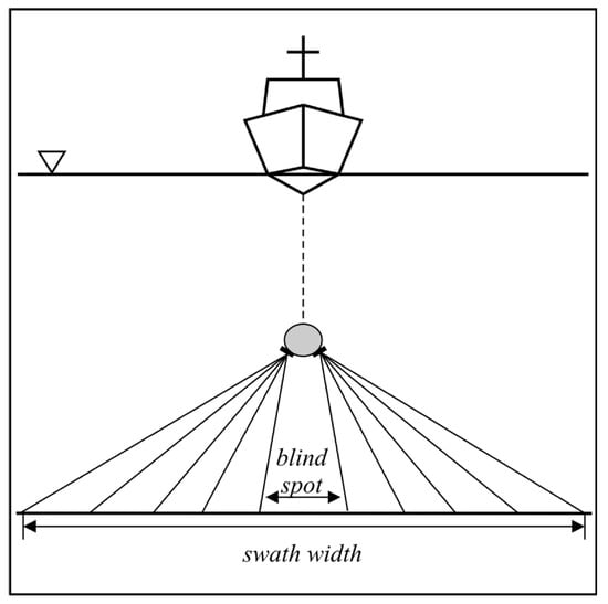 Figure 5. Side-scan sonar coverage (adapted from []).
 - Sub-bottom profilers: Contrary to the aforementioned sensors, sub-bottom profilers can obtain information from sediments and rocks under the seabed. The principle of operation is to send a low-frequency signal capable of penetrating deeper into the seabed than high-frequency signals, which are quickly absorbed due to the sound properties in the water medium. After that, the variations in acoustic impedance among distinct substrates are employed to produce the echoes []. In order to obtain a profile map, a large number of signals must be sent.
- Backscattering: Backscattering refers to the strength of the echo reflected from the bottom [,]. Different sediments and seabed structures will have different backscattering intensities. In this regard, backscattering is a helpful tool for seafloor classification. Generally, to generate acoustic images, the acoustic backscatter intensity is converted into the pixel value of a grayscale image (called the backscatter mosaic). Finally, the backscatter strength is complex data, depending on several factors, such as the incident angle of the sound waves, the roughness of the detected object/material, and the medium [,]. While side-scan sonar provides high-resolution images of the seafloor, backscattering provides data about the composition of the seabed based on the intensity of echoes.
Table 1 presents some typical variables that can be obtained from backscattering and bathymetry data. Bathymetric derivatives such as the Bathymetric Position Index (BPI) and rugosity have shown close relations with benthic ecosystem processes such as shelter availability and species abundance []. Backscatter statistics are used to classify seabed sediments regarding textural information [].

Table 1.
Backscatter statistics and bathymetric derivatives commonly found in the literature (adapted from []).
3.2. Optical Sensors
The most common optical sensors for underwater seafloor classification are cameras. They can deliver various visual data at high spatial and temporal resolutions, such as color, intensity, texture, and contours. Camera models map 3D world point spaces as two-dimensional (2D) image representations. The pinhole projective model is the most common camera model used in this context. Generally, cameras are calibrated in order to obtain the extrinsic and intrinsic parameters []. With these parameters, it is possible to define the intrinsic properties of the camera and also its position in the world against a previously defined coordinate system. However, considering the underwater environment, subaquatic images present high distortion due to the air–glass–water refraction. Figure 6 presents a simple scheme of the refraction caused by the air–glass–water interface. It is noted that an angular deviation occurs when the light beam passes through two media with different refractive indices [].
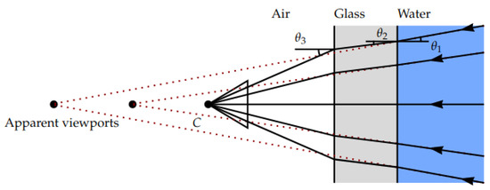
Figure 6.
Simple scheme of refraction caused by the air–glass–water interface (adapted from []).
According to Snell’s Law [], the incident and emergent angles are given by Equation (2).
Since that the emergent angle , the scene image will look wider.
Regarding sensor classification, 3D optical sensors are often divided regarding their measuring method: time of flight, triangulation, and modulation [].
- Time of flight: These sensors use Equation (1) to calculate the depth of a point. A light ray is emitted, and the time until its reception is measured. To determine the 3D position, the point position in all three axes must be located. There are three configurations to obtain the spatial configuration: a single detector used with a punctual light source steered in 2D; a 1D array of detectors with a linear light source swept in 1D; and a 2D array of detectors to capture information about a scene illuminated by diffuse light.One example of time-of-flight-based optical sensors is Pulse-Gated Laser Line Scanning (PG-LLS). The main principle of the PG-LLS sensor is illuminating a small area with a laser light pulse while keeping the receiver’s shutter closed. After that, the object distance is estimated by measuring the time it takes for the light to return. Furthermore, it captures only the light reflected from the target by opening the receiver’s shutter.
- Triangulation: Triangulation methods rely on measuring the distance between multiple devices to a common target with known parameters. One drawback of triangulation sensors is the requirement of an overlapping region between the emitters’ and receivers’ fields of view. Additionally, nearby features have a larger disparity, hence presenting better z resolution for closer distances. Moreover, the camera baseline affects the z resolution of the device. Structured Light Systems (SLSs) are one of the multiple technologies that utilize triangulation to calculate 3D information. These sensors usually consist of a camera and a projector. Knowing both the planes and camera rays (see Figure 7), a known pattern, commonly a set of light planes, is projected onto the scene. Binary patterns are typically used due to simple processing and ease of use. Binary patterns employ only two states of light, with white light being one of the most common representations.Another type of Structured Light Systems is Laser-based Structured Light Systems (LBSLSs). In these sensors, a laser plane pattern is projected onto the scene. In addition, the projector is swept across the camera’s field of view. As a result, a motorized element is required besides the laser system. Furthermore, it is mandatory to know the camera and laser’s relative position and orientation to carry out the triangulation process.
- Modulation: Regarding modulation-based sensors, they use the frequency domain to discern multiple scattered, diffused photos by using the differences in the amplitude and phase of a modulated signal. For instance, a modulated laser line scanning (LLS) system utilizes the frequency domain rather than the spatial or temporal domain to detect changes in the transmitted signal. Since amplitude modulation is the only viable modulation technique for underwater scenarios, the original and returned signals are subtracted, and the distance is calculated by demodulating the remainder.
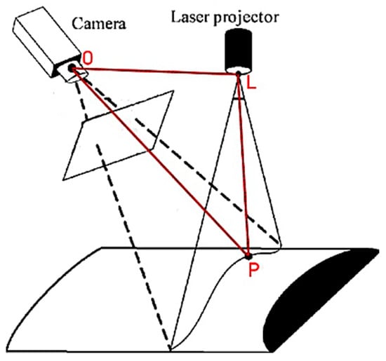
Figure 7.
Triangulation geometry principle for a Structured Light System (adapted from []).
3.3. Hyperspectral Imaging
Recent advances in hyperspectral sensing and related technologies have allowed these sensors to be employed in several marine robotic tasks, such benthic mapping, mineral exploration, and environmental monitoring []. Hyperspectral imaging differs from conventional red–green–blue (RGB) cameras by capturing the spectral composition of incident light, generating an image with additional information. Hence, hyperspectral imaging systems are able to obtain a large amount of data, gathering data across the electromagnetic spectrum. There are two main scanning approaches, namely:
- Whisk-broom scanner: Uses several detector elements, and the scanning is carried out in the cross-tracking direction by using rotating mirrors. In order to avoid image distortion, this approach is preferably used in the case of robotic vehicles operating at low speeds [].
- Push-broom scanner: In contrast to the whisk-broom method, push-broom scanners do not need a rotating element. These sensors capture an entire line in their field of view, obtaining multiple across-track wavelengths []. Conversely, it requires a higher calibration effort in order to ensure accurate data.
3.4. Other Sensors
Although acoustic and optical sensors are the main sensors used to perform seafloor classification, it is important to mention other sensors, namely seismic and magnetic. In the context of deep sea mining, for example, deploying seafloor seismometers can improve the knowledge of magnetic and hydrothermal volcanic sources in coastal and off-shore regions []. By analyzing and comparing ongoing seismic and gravitational data, it is possible to verify the presence of hydrothermal activity. Seismic data can also be used to generate numerical models that simulate the convection of seawater and thermodynamic properties [].
On the other hand, magnetic sensors can provide insights regarding sub-seafloor properties, such as magnetization and conductivity []. Usually, magnetic sensors use magnetometers or magnetic gradient meters to sense variation in magnetic signals []. The development of perception methods for magnetic sensing is influenced by the task in which they are applied. For instance, the simple processing of detected magnetic fields can be used for buried underwater mines detection, as described in Clem et al. []. In addition, for more advanced methods, Hu et al. [] use magnetic gradient tensors to localize multiple underwater objects.
4. Related Work
This section presents an overview of related work in the field of seabed classification. Each subsection introduces the theoretical background of the technique and the main results presented in the literature.
4.1. Statistical
Simons and Snellen [] introduced a Bayesian method for seafloor classification using MBES-averaged backscatter data per beam at a single angle. The study area was at Stanton bank area, located north of Ireland. First, a nonlinear curve-fitting algorithm is applied to the histogram of measured backscatter strengths in order to fit a model. Once the probability distribution function for each seafloor type has been determined, the data are subjected to classification using the Bayes decision rule. The Bayesian classification was used through the assumption that the backscatter intensities followed a Gaussian distribution. Alevizos et al. [] improved this approach by simultaneously using a combination of beams to obtain the optimal number of classes for unsupervised classification. Furthermore, this method can be used as a reliable tool for long-term environmental monitoring [].
Later, Gaida et al. [,] proposed the use of multi-frequency backscatter data collected from MBES in the Cleaver Bank area, located on the west coast of the Netherlands. The authors employed a Bayesian approach for the classification of seabed substrates using multi-frequency backscatter data. In their results, the use of multiple frequencies was demonstrated to significantly improve the acoustic discrimination of seabed sediments in comparison to single-frequency data.
Fakiris et al. [] used an MBES and a dual-frequency side scan SONAR. The data were combined to map shallow benthic habitats of the National Marine Park of Zakynthos, Greece. To mitigate the overfitting of the feature space, supervised classification was carried out utilizing a Naive Bayes classifier. It was observed that the identification of seagrass was influenced by the operating frequency, indicating the discriminatory capability of a multi-frequency dataset. Table 2 summarizes the presented approaches.
Table 2.
Recent statistical-based approaches.
4.2. Machine Learning
There are multiple methods in the literature based on conventional machine learning algorithms. These approaches range from kernel methods and decision trees to neural networks. A brief description of those strategies is presented as follows for better comprehension.
- Support Vector Machine (SVM): The main concept for the SVM algorithm is defining a hyperplane in an n-dimensional space in order to perform data classification. Given the defined hyperplane, the support vectors are determined as the closest data points, i.e., points that are on the margin of the hyperplane. The method only uses the closest samples to the hyperplane. Thus, by maximizing the margin distance from the hyperplane to the supports in the learning process, the decision boundary is determined. Generally, SVM is used for classification tasks but can also be performed for regression problems [,]. Conversely, this approach can lead to greater training time and less effectiveness for larger datasets or overlapping classes.
- Random Forest (RF): The RF algorithm involves several decision trees uncorrelated with each other that generate a final prediction through a majority vote. Recursive partitioning divides the input data into multiple regions at each decision tree. Additionally, the cutoff thresholds used in the partitioning step are obtained by learning subsets of training data chosen uniformly from the training dataset. This procedure occurs for each decision tree [,]. Typically, two parameters are defined to obtain an RF model: the number of trees and predictor variables.
- The k Nearest Neighbor (kNN): The kNN classification method is a simple algorithm that determines the class of a sample based on a majority vote of its k nearest neighbors within the training set. However, one major hindrance of this technique is its poor scalability since the model must keep the complete training dataset in memory in order to make a prediction [].
Regarding recent approaches, Lawson et al. [] analyzed the performance of two machine learning algorithms to classify noisy seamount feature sets obtained from bathymetry data: Random Forests (RFs) and Extremely Randomized Trees. In the authors’ study, the feature metrics used were slope, aspect, plan curvature, profile curvature, and fractal dimension. In their analysis, the Extremely Randomized Trees presented the best results, with 97% accuracy. The results suggested that topography is the most important data representation for classification tasks.
Ji et al. [] proposed a Selecting Optimal Random Forest (SORF) algorithm for seabed classification. The research region is situated along the southern shoreline of the Jiaodong Peninsula. First, the authors applied the pulse-coupled neural network image-enhancement model to improve the MBES image quality. Besides seafloor topography, seabed roughness was also considered in the feature extraction algorithm. A total of 40 features were obtained to improve the intensity description. By using the SORF, the author’s method can automatically select input features and optimize model parameters to further improve classification efficiency and accuracy. The model is compared with RF and SVM classifiers. The results showed that the proposal outperforms the RF and SVM, in addition to having better computational efficiency for high-dimensional features.
Ji et al. [] used a Back-Propagation Neural Network (BPNN) as a classifier for seabed sediments with MBES backscatter data obtained at the Jiaozhou Bay, China. The study selected 8 out of the 34 extracted dimensions of the initial feature vector in order to reduce workload, hence enhancing efficiency and accuracy. The authors proposed multiple optimization techniques, including Particle Swarm Optimization (PSO) and Adaptive Boosting (AdaBoost), to prevent the network from getting trapped in local minimums. These optimization methods can lead to better results. In their experiments, the authors combined both optimization methods with the BPNN classifier and compared them to SVM models and a one-level decision tree, achieving better accuracy.
Zhao et al. [] used the Weyl Transform to characterize backscatter imagery provided by MBES obtained in the Belgian section of the North Sea. The authors’ proposal focused on the textural analysis of seafloor sediments and used the Weyl Transform to obtain the features. The method divides the acoustic images into patches and carries out the feature extraction for each patch. The used dataset corresponded to four types of sediments: sand, sandy mud, muddy sand, and gravelly sand. Finally, a Random Forest classifier was designed to classify the features.
Zelada Leon et al. [] assessed the repeatability of seafloor classification algorithms using data from the Greater Haig Fras area, in the southern part of the Celtic Sea. In the authors’ study, three classifiers were used: RF, KNN, and K-means. Based on the results, only the RF and KNN algorithms were statistically repeatable, with the Random Forest approach being the more robust. In the low-relief test area, backscatter statistics obtained from the side-scan sonar had more importance than the bathymetric derivatives for seabed sediments classification.
Generally, techniques based on optical sensors are based on computer vision. Traditional ML algorithms involved the design of hand-crafted features, such as shape, color, or texture features []. For instance, Beijbom et al. [] extracted texture and color features from underwater corals based on an SVM classifier. Similarly, Villon et al. [] used an SVM model to detect fish in coral reefs.
Dahal et al. [] compared Logistic Regression, KNN, Decision Trees, and RF models on a coral reef monitoring dataset. In the experimental results, the RF presented the best results. However, the authors stated that the parameters chosen can significantly impact the performance of each model.
Mohamed et al. [] proposed a methodology for the 3D mapping and classification of benthic habitats. First, the video recordings, obtained at Ishigaki Island, Japan, were converted into geolocated images, and each was labeled manually. Then, the Bagging of Features, Hue Saturation Value, and Gray Level Co-occurrence Matrix algorithms were applied in order to obtain image attributes. Given the image attributes, the authors trained three machine learning classifiers, namely KNN, SVM, and bagging. The outputs of these classifiers were combined using the fuzzy majority voting algorithm. The Structure from Motion and Multi-View Stereo algorithm is applied to generate 3D maps and digital terrain models of each habitat. Table 3 presents related work regarding machine learning techniques.
In order to explore high-resolution imagery, Dumke et al. [] applied an SVM to detect manganese nodules in image data provided by an underwater hyperspectral camera. The survey was carried out at the Peru Basin, southeast of the Pacific Ocean. The SVM was compared with a spectral angle mapper approach, with the former presenting better results.
Table 3.
Recent machine-learning-based approaches.
Table 3.
Recent machine-learning-based approaches.
| Reference | Year | Data Type | Task | Sensors Type | Technique |
|---|---|---|---|---|---|
| Lawson et al. [] | 2017 | Bathymetry | Seamounts Features Classification | MBES | RF and Extremely Randomized Trees |
| Ji et al. [] | 2020 | Backscattering | Seafloor Sediment Classification | MBES | SORF, RF, SVM |
| Ji et al. [] | 2020 | Backscattering | Seafloor Sediment Classification | MBES | BPNN, SVM |
| Cui et al. [] | 2021 | Backscattering and Bathymetry | Seafloor mapping | MBES | SVM |
| Zhao et al. [] | 2021 | Backscattering | Seafloor Sediment Classification | MBES | RF |
| Zelada Leon et al. [] | 2020 | Backscattering and Bathymetry | Seafloor Sediment Classification | Side-scan | RF |
| Beijbom et al. [] | 2012 | RGB Images | Coral Reef Annotation | Camera | SVM |
| Dahal et al. [] | 2021 | RGB Image | Coral Reef Monitorting | Camera | Logistic Regression, KNN, Decision Tree, and RF |
| Mohamed et al. [] | 2020 | RGB Image | Benthic Habitats Mapping | Camera | SVM, KNN |
| Dumke et al. [] | 2018 | Spectral Image | Manganese Nodules Mapping | Hyperspectral Camera | SVM |
4.3. Deep Learning
Convolutional Neural Networks (CNNs) have been extensively used in computer vision due to their performance. The key concept of CNNs is the use of multiple layers of feature detectors to automatically identify and learn patterns within the data. The hidden layer of a CNN typically comprises three components: the convolutional layer, where feature extraction occurs through convolution with filter matrices followed by activation using Rectified Linear Units (ReLU); the pooling layer, which reduces dimensionality by aggregating the output of the ReLU layer, thus enhancing computational efficiency; and the fully connected layer, which learns nonlinear combinations of features acquired from previous layers [,].
Considering object detection, state-of-the-art architectures are divided into two types: one-stage and two-stage. Two examples of one-stage approaches are SSD (Single-Shot multi-box Detector) and You Only Look Once (YOLO), which use a CNN to obtain prediction-bounding boxes along probabilities for objects’ classes [].
SSD comprises a backbone model, typically a pre-trained image classification network serving as a feature extractor, and an SSD head, consisting of additional convolutional layers interpreting outputs as bounding boxes and object classes. YOLO, in contrast, generates multiple bounding boxes per object and suppresses redundant boxes to obtain final coordinates [,].
On the other hand, two-stage detectors have a stage for the proposal of regions of interest. First, regions of interest with potential objects are proposed. Subsequently, the second stage performs object classification. Examples of these architectures are the Fast R-CNN, Faster R-CNN, and Mask R-CNN [,].
Regarding deep learning approaches, Luo et al. [] studied the feasibility of CNNs for sediment classification in a small side-scan sonar dataset of the Pearl River Estuary in China. To achieve this, the authors used a modified shallow CNN pre-trained on LeNet-5 [] and a deep CNN modified based on AlexNet []. The dataset contained three classes (reefs, sand waves, and mud), and, for classification purposes, the acoustic images were divided into small-scale images. The numbers of classified reef, mud, and sand wave images were 234, 217, and 228, respectively. From each sediment type, 20% of the images were randomly selected as test samples: 46, 43, and 45 images of reef, mud, and sand waves. The results showed that the shallow CNN had better performance than the deep CNN, achieving 87.54%, 90.56%, and 93.43% accuracy for reefs, mud, and sand wave on the testing dataset, respectively. Later, Qin et al. [] used common CNNs, such as AlexNet-BN, LeNet-BN, VGG16, and others, to classify seabed sediments in a small side-scan sonar dataset. The model was pre-trained on the grayscale CIFAR-10 dataset containing 10 classes of images with almost no similarity to the sonar images. Data enhancement based on Generative Adversarial Network (GAN) was carried out, thus expanding the dataset. The authors applied a conditional batch normalization and altered the loss function in order to enhance the stability of the GAN. Finally, the proposal was compared with the SVM classifier. The results showed that data-optimization techniques can overcome the problem of small datasets in sediment classification. However, the use of GAN is computationally expensive. The authors suggested that fine-tuning the CNNs is fundamental in small datasets.
Jie et al. [] presented an Artificial Neural Network (ANN) with a two-hidden-layer feed-forward topology network to estimate polymetallic nodule abundance using side-scan backscatter from the Clarion and Clipperton Fracture Zone (CCFZ) in the Pacific Ocean, obtaining average accuracy of 84.20%. Later, the method was improved by Wong et al. [] by adding bathymetry data. Their proposal aimed to determine the correlation of side-scan sonar backscatter and terrain variations. Assuming a constant density of nodules in the bathymetry pixels, variations in bathymetry can indicate the density and abundance of nodules. The ground truth labels for the ANN were estimated from seabed photographs. The results using the testing dataset presented an accuracy of 85.36%, demonstrating that combining backscatter and bathymetry data can improve the performance. However, the network was not tested on a different dataset.
State-of-the-art deep learning models have also been used to classify objects in acoustic images. Aleem et al. [] proposed the use of the Faster R-CNN architecture to classify submerged marine debris in a forward-looking sonar dataset captured at a lab water tank. In order to improve the model performance, the authors proposed a median filter and histogram equalization for noise removal. A transfer learning approach was used by combining the Faster R-CNN with ResNet 50 for feature extraction.
The one stage model YOLOv5s was used by Yu et al. [] for real-time object detection in side-scan sonar images. First, the authors down-sampled the echoes of the images while keeping the aspect ratio between the along-track direction and the cross-track direction. The aim of the downsampling technique employed is to improve recognition accuracy while reducing computational costs. During the network training, transfer learning was used by pre-training the model on the COCO dataset. Similarly, Zhang et al. [], proposed YOLOv5s pre-trained on the COCO dataset for target detection in a forward-looking sonar dataset. In their proposal, the k-means clustering algorithm was used to fine-tune the network.
Dong et al. [] used Mask R-CNN pre-trained on the COCO dataset to segment deep sea nodule minerals in camera images. The performance of the network was compared to that of other learning models, such as U-Net and GAN. The dataset comprised 106 images of nodules with diverse abundance and environmental conditions. The authors stated that due to the similarities of the nodules and the seafloor sediments, image processing methods, including threshold segmentation, clustering segmentation, and multispectral segmentation, cannot distinguish them. When compared with the U-Net and GAN models, the Mask R-CNN had better performance in terms of three metrics: accuracy (97.245%), recall (85.575%), and IoU (74.728%).
Quintana et al. [] proposed an algorithm to detect manganese nodules automatically. The dataset comprised data obtained at the Peru basin in the Pacific Ocean. First, potential areas with nodules are identified using bathymetry data provided by an MBES. Then, visual detection is carried out. The images are filtered in order to reduce noise and apply lighting corrections. For comparison, two state-of-the-art models are used, YOLO and Fast R-CNN, with the latter presenting better performance. Initial nodule images were obtained in preliminary pool experiments, and the algorithms were able to detect nodules in situ [,].
Fulton et al. [] developed the Trash-ICRA19, a marine litter dataset, for robotic detection composed of approximately 5700 images obtained in the Sea of Japan. The dataset defines three classes: rov (man-made objects), bio (fish, plants, and biological deposits generally), and plastic (marine debris). For evaluation, the authors applied the YOLOv2, tiny YOLOv2, SSD, and Faster R-CNN models. The algorithms were executed on NVIDIA Jetson TX2, and the results indicate that those architectures can potentially be used to detect marine litter disposed on the seafloor in real time. The performance metrics utilized to assess the networks were Mean Average Precision (mAP) and Intersection Over Union (IoU). Considering litter detection, the mAP values for the YOLOv2, tiny YOLOv2, SSD, and Faster R-CNN models were 47.9%, 31.6%, 67.4%, and 81.0%, respectively. The IoU results were 54.7%, 49.8%, 60.6%, and 53%. A new version of the dataset called TrashCan was presented by Hong et al. []. Compared to the previous version, this dataset is more varied, containing more images and classes, and the Mask R-CNN and Faster R-CNN models were used as a baseline. Table 4 summarizes recent approaches based on deep learning.
Table 4.
Recent deep-learning-based approaches.
4.4. Object-Based Image Analysis (OBIA)
OBIA is a feature-extraction technique comprising two stages: segmentation and feature extraction. In the segmentation step, pixels with similar spectral, spatial, and contextual characteristics are grouped together to define objects, as described by Hossain and Chen []. Then, a feature extraction or classification algorithm is used on the objects.
Menandro et al. [] applied a supervised classification technique called OBIA in side-scan sonar backscatter data in order to perform seabed reef mapping. The evaluated data were gathered in the continental shelf of Abrolhos, located in the eastern region of Brazil. OBIA defines image/vector objects, which are sets of image pixels arranged into different levels. At the pixel level, image objects are identical to the pixels themselves. Segmenting the image starting from the pixel level results in a higher level of image objects known as “Fine”, which can be further segmented to create “Medium” and “Coarse” levels of image objects. Moreover, statistics can be computed for each image object to generate image object features. Then, those features are used for classification. Then, the authors compared the OBIA approach with the morphometric classification method benthic terrain modeler (obtained from MBES bathymetry) and a mix of both. The results showed that both overestimated the reef area compared to the reference map, with the OBIA method presenting 67.1% alignment while the benthic terrain modeler approached 69.1%. Conversely, the combination of techniques presented improved results, achieving alignment of 75.3% with the reference dataset.
Another OBIA approach is presented by Koop et al. []. The authors proposed two methods that only use bathymetry and bathymetric derivatives to classify the seafloor sediments. The first is based on textural analysis and uses only texture-related image object features, while the second method utilizes additional image object features. In their experiments, the latter algorithm had better performance, with classification accuracy of 73%, and 87%, respectively. Besides this, the authors also analyzed the transferability of their proposal by testing it on different datasets (Røstbanken area, Norway, and Borkumer Stones, Netherlands), finding that the method remains applicable to new datasets as long as image objects are allowed to conform to the shapes of small-scale seafloor features at lower levels.
Janowski et al. [] applied an OBIA approach for nearshore seabed benthic mapping based on multi-frequency multibeam data gathered at the Rowy site in the southern Baltic Sea. The authors’ method was able to distinguish six nearshore habitats using backscattering and bathymetry data. The results were compared to traditional ML approaches such as Random Forest and k-Nearest Neighbors. Table 5 displays the discussed approaches.
Table 5.
Recent OBIA-based approaches.
4.5. Data Generation
Due to the challenge of underwater environments and the difficulty of obtaining ground truth data, another research direction that has been explored is data generation, i.e., applying techniques to create synthetic data. These synthetic data are then used to improve the performance of classification algorithms. The main techniques presented in the literature are as follows
- Generative Adversarial Networks: GANs are a type of neural network that consists of two components. The generator component is trained to replicate the patterns found in the input data, thereby producing synthetic data points as output. On the other hand, the discriminator component is trained to differentiate between input data from the real dataset and synthetic data generated by the generator. Both components are trained in parallel, and the training process stops once the discriminator accurately classifies most of the generated data as real [].
- Autoencoder (AE) Neural Network: normally stacks two identical neural networks to generate an output that aims to replicate the input data. Initially, the autoencoder converts the input data vector into higher- or lower-dimensional data representation. The encoder network encodes the data and produces intermediate embedding layers as compressed feature representations. In addition, the decoder network takes the value from the embedding layer as input and reproduces the original input []. The lower-dimensional encoded data are often denoted as latent space.
Table 6 summarizes the related work to data generation. Kim et al. [] introduced a novel approach involving the application of an AE for the purpose of mitigating noise in SONAR images. This approach enabled the generation of a high-quality image dataset derived from SONAR images by implementing the learned AE structures.
Table 6.
Recent techniques for data generation.
Kim et al. [] proposed a data-augmentation procedure based on CNN and discrete wavelet transform. The authors’ algorithm convolves an acoustic signal and an impulse response signal and subsequently introduces white Gaussian noise to generate extended signals. Finally, a comprehensive dataset comprising 30,000 images belonging to 30 distinct categories of underwater acoustic signals was produced.
In the literature, GANs models have been used to generate synthetic images, which can overcome the issues caused by the typical scarcity of acoustic images in datasets. For instance, Phung et al. [] employed a GAN model to produce additional sonar images to increase the training dataset of a hybrid CNN and Gaussian process classifier. The network’s classification rate increased by 1.28% when trained with the augmented dataset, achieving a total of 81.56%. Jegorova et al. [] were able to accurately replicate the data distortions obtained by a moving vessel.
5. Discussion
Most of the presented works related to seabed classification and mapping tasks use acoustic sensors. This is due to the fact that these sensors present a higher sensing range despite the lower resolution. Optical sensors, on the other hand, are limited due to their generally small field of view and effective range. The majority of supervised techniques rely on traditional ML algorithms and require significant labeled data. Furthermore, these strategies depend on the thorough preprocessing of the collected data to achieve optimal outcomes. However, these processing tasks can be computationally intensive and may hinder the feasibility of real-time solutions. Moreover, ground-truth sampling can be a difficult task, as in deep sea scenarios.
Nevertheless, there is a lack of acoustic data from echosounders, particularly data that have been labeled. Some authors have tackled this issue by using synthetic images or data-augmentation techniques [,,,]. One advantage of using synthetic data is enabling the training of other models by transfer learning. However, few studies analyze the transferability of their models.
Traditional machine learning techniques are normally used for classification tasks for both acoustic data and optical images. Considering vision-based techniques, state-of-the-art architectures [,,,,] have been shown to be effective for object detection. However, in the case of underwater robotics, it is necessary to have great computational power to run these models. In this sense, there is a scarcity of approaches that seek to develop lightweight models. Furthermore, these approaches are limited by the cameras’ field of view, requiring vehicles to be close to the target to be detected. Conversely, considering the presence of other sensors attached to the vehicle, it is difficult to obtain the optimal distance so that the approach to the seafloor does not affect the performance of the other sensors.
Considering deep learning approaches, the models are usually dependent on the relationships between training datasets and the object domain. Additionally, few specify the ability of the proposal to operate in real-time scenarios, with many presenting offline post-processing approaches.
5.1. Challenges
Currently, one of the main drawbacks to deep sea research is the lack of data diversity and massive datasets. Although there are a large number of datasets in the literature, such as images of coral reefs [,], marine debris [,], marine animals [,,], or acoustic datasets [,], these datasets are for object detection and are simple in the sense that they are task-dependent. Moreover, they correspond to only one modality, making a multimodal approach impossible. Datasets such as the ETOPO 2022 [] are designed to create a global relief elevation model. However, it is not appropriate for characterizing specific objects such as marine litter, polymetallic nodules, corals, and other classes. The Aurora dataset [] is one of the first attempts to create a multimodal dataset. However, the samples are not annotated, which makes the annotation process exhaustive.
Besides this, the size of the targets presents another challenge for underwater object-detection tasks []. In vision-based systems, for example, detection algorithms are not able to obtain discriminative features for small objects. Additionally, the objects tend to gather in dense distributions (manganese nodules and corals).
The more recent approaches are mainly based on deep learning. An important factor to consider for deep learning models is the consumption of computational and energy resources, particularly for small mobile robots, which may necessitate significant optimization for optimal functionality. In order to enhance the efficiency of inference processing, every opportunity for parallelization must be explored, even in the absence of GPU hardware, which is frequently the case with these robots. The efficient deployment of learning-based algorithms is closely linked to the available hardware.
Another challenge for DL models in underwater environments relates to their ability to adapt to new data. Considering the large heterogeneity of the seafloor, there is a large discrepancy between different areas of the ocean, creating a major generalization problem. For instance, object-detection models suffer a great loss of accuracy when applied to other domains [].
5.2. Future Directions
Besides the challenges already presented in the discussion, there are still areas to be explored.
- Multimodal Dataset: One of the main challenges to improving the performance of the algorithms presented in the dataset used. In this regard, the generation of a multimodal and public dataset could be a powerful tool for improving seabed characterization approaches, thus overcoming some challenges, such as obtaining ground truth, specifically in deep sea scenarios, unbalanced data, and others.
- Multimodal learning: Multimodal learning means applying ML and DL techniques to fuse multisource data with different modalities, obtaining more complete and accurate features. However, other challenges arise when attempting to integrate sensors from different modalities. The maximum range is different for optical and acoustic sensors. For instance, optical sensors have lower ranges than acoustic ones, and the vehicle must be close to the seabed to obtain images. Furthermore, the sensors have different temporal and spatial resolutions, which can hinder data alignment and, hence, data fusion. Recently, there has been an increase in research using multimodal fusion in underwater environments. For instance, Ben Tamou et al. [] proposed a hybrid fusion that combines appearance and motion information for automatic fish detection. The authors employed two Faster R-CNN models that shared the same region proposal network. Farahnakian and Heikkonen [] proposed three methods for multimodal fusion of RGB images and infrared data to detect maritime vessels. Two architectures are based on early fusion theory, including pixel-level and feature-level fusion.
- Edge Intelligence (EI): EI is a recent paradigm that has been widely researched [,,]. The main idea is to bring all data processing close to where the data are gathered. In the literature, some studies presented definitions for EI. For instance, Zhang et al. [] define edge intelligence as the capability to enable edges to execute artificial intelligence algorithms. EI leverages multimodal learning algorithms by enabling real-time processing, leading to the development of novel techniques for several applications. EI can enable the neural network to be trained while the data are being gathered [,].
6. Conclusions
This survey presented papers related to seabed characterization. The challenges associated with this topic were presented. Moreover, it was noted that several approaches can be used to tackle this problem. However, there is a trend toward the use of deep learning techniques, mainly based on CNNs.
The ability to perceive and characterize the elements present in the sea floor is crucial for several robotic applications. Despite recent advances, some challenges remain, such as the lack of a public dataset that can serve as a benchmark and the capacity of the developed methods to be applied to different systems. Finally, there are still paths to be explored, such as multimodal fusion. Multimodal learning may be able to obtain a better feature representation from multiple sensors when compared to a single modality. Another potential direction concerns the use of edge intelligence to improve seabed classification. By bringing data processing closer to the sources, certain advantages appear, such as real-time processing and the possibility of making decisions.
Author Contributions
Conceptualization, G.L.; methodology, G.L.; software, G.L.; validation, G.L.; formal analysis, G.L.; investigation, G.L.; resources, E.S.; data curation, G.L.; writing—original draft preparation, G.L.; writing—review and editing, G.L., A.D., J.A., A.M., S.H. and E.S.; visualization, G.L.; supervision, A.D., J.A., A.M., S.H. and E.S.; project administration, E.S.; funding acquisition, E.S. All authors have read and agreed to the published version of the manuscript.
Funding
This work was funded by TRIDENT project financed by the European Union’s HE programme under grant agreement No 101091959.
Data Availability Statement
No new data were created or analyzed in this study. Data sharing is not applicable to this article.
Acknowledgments
The authors would like to thank the Portuguese funding agency, FCT—Fundação para a Ciência e a Tecnologia, under the research grant 2021.08715.BD.
Conflicts of Interest
The authors declare no conflicts of interest.
Abbreviations
The following abbreviations are used in this manuscript:
| AdaBoost | Adaptive Boosting |
| AE | AutoEncoder |
| ANN | Artificial Neural Network |
| AUV | Autonomous Underwater Vehicle |
| BPNN | Back-Propagation Neural Network |
| CCFZ | Clarion and Clipperton Fracture Zone |
| CNN | Convolutional Neural Network |
| DL | Deep Learning |
| GAN | Generative Adversarial Network |
| kNN | K Nearest Neighbours |
| LBSLS | Laser-based Structured Light Systems |
| MBES | Multibeam Echosounder |
| MDPI | Multidisciplinary Digital Publishing Institute |
| ML | Machine Learning |
| OBIA | Object-based Image Analysis |
| PG-LLS | Pulse Gated Laser Line Scanning |
| PSO | Particle Swarm Optimization |
| RF | Random Forest |
| RBG | red-green-blue |
| SONAR | Sound Navigation and Ranging |
| SORF | Selecting Optimal Random Forest |
| SSD | Single-Shot multi-box Detector |
| SVM | Support Vector Machine |
| YOLO | You Only Look Once |
References
- Costello, M.J.; Chaudhary, C. Marine biodiversity, biogeography, deep sea gradients, and conservation. Curr. Biol. 2017, 27, R511–R527. [Google Scholar] [CrossRef] [PubMed]
- Danovaro, R.; Fanelli, E.; Aguzzi, J.; Billett, D.; Carugati, L.; Corinaldesi, C.; Dell’Anno, A.; Gjerde, K.; Jamieson, A.J.; Kark, S.; et al. Ecological variables for developing a global deep-ocean monitoring and conservation strategy. Nat. Ecol. Evol. 2020, 4, 181–192. [Google Scholar] [CrossRef] [PubMed]
- Boomsma, W.; Warnaars, J. Blue mining. In Proceedings of the 2015 IEEE Underwater Technology (UT), Chennai, India, 23–25 February 2015; pp. 1–4. [Google Scholar]
- Galparsoro, I.; Agrafojo, X.; Roche, M.; Degrendele, K. Comparison of supervised and unsupervised automatic classification methods for sediment types mapping using multibeam echosounder and grab sampling. Ital. J. Geosci. 2015, 134, 41–49. [Google Scholar] [CrossRef]
- Cong, Y.; Gu, C.; Zhang, T.; Gao, Y. Underwater robot sensing technology: A survey. Fundam. Res. 2021, 1, 337–345. [Google Scholar] [CrossRef]
- Sun, K.; Cui, W.; Chen, C. Review of underwater sensing technologies and applications. Sensors 2021, 21, 7849. [Google Scholar] [CrossRef] [PubMed]
- Wölfl, A.C.; Snaith, H.; Amirebrahimi, S.; Devey, C.W.; Dorschel, B.; Ferrini, V.; Huvenne, V.A.; Jakobsson, M.; Jencks, J.; Johnston, G.; et al. Seafloor mapping–the challenge of a truly global ocean bathymetry. Front. Mar. Sci. 2019, 6, 283. [Google Scholar] [CrossRef]
- Hou, S.; Jiao, D.; Dong, B.; Wang, H.; Wu, G. Underwater inspection of bridge substructures using sonar and deep convolutional network. Adv. Eng. Inform. 2022, 52, 101545. [Google Scholar] [CrossRef]
- Wu, Y.; Ta, X.; Xiao, R.; Wei, Y.; An, D.; Li, D. Survey of underwater robot positioning navigation. Appl. Ocean. Res. 2019, 90, 101845. [Google Scholar] [CrossRef]
- Wang, X.; Müller, W.E. Marine biominerals: Perspectives and challenges for polymetallic nodules and crusts. Trends Biotechnol. 2009, 27, 375–383. [Google Scholar] [CrossRef] [PubMed]
- Hein, J.R.; Koschinsky, A.; Kuhn, T. Deep-ocean polymetallic nodules as a resource for critical materials. Nat. Rev. Earth Environ. 2020, 1, 158–169. [Google Scholar] [CrossRef]
- Kang, Y.; Liu, S. The development history and latest progress of deep sea polymetallic nodule mining technology. Minerals 2021, 11, 1132. [Google Scholar] [CrossRef]
- Leng, D.; Shao, S.; Xie, Y.; Wang, H.; Liu, G. A brief review of recent progress on deep sea mining vehicle. Ocean. Eng. 2021, 228, 108565. [Google Scholar] [CrossRef]
- Hein, J.R.; Mizell, K. Deep-Ocean Polymetallic Nodules and Cobalt-Rich Ferromanganese Crusts in the Global Ocean: New Sources for Critical Metals. In Proceedings of the United Nations Convention on the Law of the Sea, Part XI Regime and the International Seabed Authority: A Twenty-Five Year Journey; Brill Nijhoff: Boston, MA, USA, 2022; pp. 177–197. [Google Scholar]
- Sparenberg, O. A historical perspective on deep sea mining for manganese nodules, 1965–2019. Extr. Ind. Soc. 2019, 6, 842–854. [Google Scholar] [CrossRef]
- Miller, K.A.; Thompson, K.F.; Johnston, P.; Santillo, D. An overview of seabed mining including the current state of development, environmental impacts, and knowledge gaps. Front. Mar. Sci. 2018, 4, 418. [Google Scholar] [CrossRef]
- Santos, M.; Jorge, P.; Coimbra, J.; Vale, C.; Caetano, M.; Bastos, L.; Iglesias, I.; Guimarães, L.; Reis-Henriques, M.; Teles, L.; et al. The last frontier: Coupling technological developments with scientific challenges to improve hazard assessment of deep sea mining. Sci. Total Environ. 2018, 627, 1505–1514. [Google Scholar] [CrossRef] [PubMed]
- Toro, N.; Jeldres, R.I.; Órdenes, J.A.; Robles, P.; Navarra, A. Manganese nodules in Chile, an alternative for the production of Co and Mn in the future—A review. Minerals 2020, 10, 674. [Google Scholar] [CrossRef]
- Thompson, J.R.; Rivera, H.E.; Closek, C.J.; Medina, M. Microbes in the coral holobiont: Partners through evolution, development, and ecological interactions. Front. Cell. Infect. Microbiol. 2015, 4, 176. [Google Scholar] [CrossRef] [PubMed]
- Letnes, P.A.; Hansen, I.M.; Aas, L.M.S.; Eide, I.; Pettersen, R.; Tassara, L.; Receveur, J.; le Floch, S.; Guyomarch, J.; Camus, L.; et al. Underwater hyperspectral classification of deep sea corals exposed to 2-methylnaphthalene. PLoS ONE 2019, 14, e0209960. [Google Scholar] [CrossRef] [PubMed]
- Boolukos, C.M.; Lim, A.; O’Riordan, R.M.; Wheeler, A.J. Cold-water corals in decline–A temporal (4 year) species abundance and biodiversity appraisal of complete photomosaiced cold-water coral reef on the Irish Margin. Deep. Sea Res. Part I Oceanogr. Res. Pap. 2019, 146, 44–54. [Google Scholar] [CrossRef]
- de Oliveira Soares, M.; Matos, E.; Lucas, C.; Rizzo, L.; Allcock, L.; Rossi, S. Microplastics in corals: An emergent threat. Mar. Pollut. Bull. 2020, 161, 111810. [Google Scholar] [CrossRef]
- Brown, C.J.; Smith, S.J.; Lawton, P.; Anderson, J.T. Benthic habitat mapping: A review of progress towards improved understanding of the spatial ecology of the seafloor using acoustic techniques. Estuar. Coast. Shelf Sci. 2011, 92, 502–520. [Google Scholar] [CrossRef]
- Steiniger, Y.; Kraus, D.; Meisen, T. Survey on deep learning based computer vision for sonar imagery. Eng. Appl. Artif. Intell. 2022, 114, 105157. [Google Scholar] [CrossRef]
- Xu, S.; Zhang, M.; Song, W.; Mei, H.; He, Q.; Liotta, A. A systematic review and analysis of deep learning-based underwater object detection. Neurocomputing 2023, 527, 204–232. [Google Scholar] [CrossRef]
- Fayaz, S.; Parah, S.A.; Qureshi, G. Underwater object detection: Architectures and algorithms–a comprehensive review. Multimed. Tools Appl. 2022, 81, 20871–20916. [Google Scholar] [CrossRef]
- Liu, B.; Liu, Z.; Men, S.; Li, Y.; Ding, Z.; He, J.; Zhao, Z. Underwater hyperspectral imaging technology and its applications for detecting and mapping the seafloor: A review. Sensors 2020, 20, 4962. [Google Scholar] [CrossRef] [PubMed]
- Chutia, S.; Kakoty, N.M.; Deka, D. A review of underwater robotics, navigation, sensing techniques and applications. In Proceedings of the AIR 17: Proceedings of the 2017 3rd International Conference on Advances in Robotics, New Delhi, India, 28 June–2 July 2017; pp. 1–6. [Google Scholar]
- Wang, J.; Kong, D.; Chen, W.; Zhang, S. Advances in software-defined technologies for underwater acoustic sensor networks: A survey. J. Sens. 2019, 2019, 3470390. [Google Scholar] [CrossRef]
- Martins, A.; Almeida, J.; Almeida, C.; Matias, B.; Kapusniak, S.; Silva, E. EVA a hybrid ROV/AUV for underwater mining operations support. In Proceedings of the 2018 OCEANS-MTS/IEEE Kobe Techno-Oceans (OTO), Kobe, Japan, 28–31 May 2018; pp. 1–7. [Google Scholar]
- Duntley, S.Q. Light in the sea. JOSA 1963, 53, 214–233. [Google Scholar] [CrossRef]
- Peng, Y.T.; Cosman, P.C. Underwater image restoration based on image blurriness and light absorption. IEEE Trans. Image Process. 2017, 26, 1579–1594. [Google Scholar] [CrossRef]
- Liu, H.; Chau, L.P. Underwater image color correction based on surface reflectance statistics. In Proceedings of the 2015 Asia-Pacific Signal and Information Processing Association Annual Summit and Conference (APSIPA), Hong Kong, 16–19 December 2015; pp. 996–999. [Google Scholar]
- Roznere, M.; Li, A.Q. Real-time model-based image color correction for underwater robots. In Proceedings of the 2019 IEEE/RSJ International Conference on Intelligent Robots and Systems (IROS), The Venetian Macao, Macau, 3–8 November 2019; pp. 7191–7196. [Google Scholar]
- Yang, M.; Hu, K.; Du, Y.; Wei, Z.; Sheng, Z.; Hu, J. Underwater image enhancement based on conditional generative adversarial network. Signal Process. Image Commun. 2020, 81, 115723. [Google Scholar] [CrossRef]
- Hashisho, Y.; Albadawi, M.; Krause, T.; von Lukas, U.F. Underwater color restoration using u-net denoising autoencoder. In Proceedings of the 2019 11th International Symposium on Image and Signal Processing and Analysis (ISPA), Dubrovnik, Croatia, 23–25 September 2019; pp. 117–122. [Google Scholar]
- Liu, Y.; Xu, H.; Zhang, B.; Sun, K.; Yang, J.; Li, B.; Li, C.; Quan, X. Model-based underwater image simulation and learning-based underwater image enhancement method. Information 2022, 13, 187. [Google Scholar] [CrossRef]
- Kim, A.; Eustice, R.M. Real-time visual SLAM for autonomous underwater hull inspection using visual saliency. IEEE Trans. Robot. 2013, 29, 719–733. [Google Scholar] [CrossRef]
- Monterroso Muñoz, A.; Moron-Fernández, M.J.; Cascado-Caballero, D.; Diaz-del Rio, F.; Real, P. Autonomous Underwater Vehicles: Identifying Critical Issues and Future Perspectives in Image Acquisition. Sensors 2023, 23, 4986. [Google Scholar] [CrossRef] [PubMed]
- Lu, H.; Li, Y.; Xu, X.; Li, J.; Liu, Z.; Li, X.; Yang, J.; Serikawa, S. Underwater image enhancement method using weighted guided trigonometric filtering and artificial light correction. J. Vis. Commun. Image Represent. 2016, 38, 504–516. [Google Scholar] [CrossRef]
- Gonçalves, L.C.d.C.V. Underwater Acoustic Communication System: Performance Evaluation of Digital Modulation Techniques. Ph.D. Thesis, Universidade do Minho, Braga, Portugal, 2012. [Google Scholar]
- Milne, P.H. Underwater Acoustic Positioning Systems. 1983. Available online: https://www.osti.gov/biblio/6035874 (accessed on 2 March 2024).
- Ainslie, M.A. Principles of Sonar Performance Modelling; Springer: Cham, Switzerland, 2010; Volume 707. [Google Scholar]
- Cholewiak, D.; DeAngelis, A.I.; Palka, D.; Corkeron, P.J.; Van Parijs, S.M. Beaked whales demonstrate a marked acoustic response to the use of shipboard echosounders. R. Soc. Open Sci. 2017, 4, 170940. [Google Scholar] [CrossRef] [PubMed]
- Grall, P.; Kochanska, I.; Marszal, J. Direction-of-arrival estimation methods in interferometric echo sounding. Sensors 2020, 20, 3556. [Google Scholar] [CrossRef] [PubMed]
- Wang, X.; Yang, F.; Zhang, H.; Su, D.; Wang, Z.; Xu, F. Registration of Airborne LiDAR Bathymetry and Multibeam Echo Sounder Point Clouds. IEEE Geosci. Remote Sens. Lett. 2021, 19, 1–5. [Google Scholar] [CrossRef]
- Torroba, I.; Bore, N.; Folkesson, J. A comparison of submap registration methods for multibeam bathymetric mapping. In Proceedings of the 2018 IEEE/OES Autonomous Underwater Vehicle Workshop (AUV), Porto, Portugal, 6–9 November 2018; pp. 1–6. [Google Scholar]
- Novaczek, E.; Devillers, R.; Edinger, E. Generating higher resolution regional seafloor maps from crowd-sourced bathymetry. PLoS ONE 2019, 14, e0216792. [Google Scholar] [CrossRef]
- Amiri-Simkooei, A.R.; Koop, L.; van der Reijden, K.J.; Snellen, M.; Simons, D.G. Seafloor characterization using multibeam echosounder backscatter data: Methodology and results in the North Sea. Geosciences 2019, 9, 292. [Google Scholar] [CrossRef]
- Collier, J.; Brown, C.J. Correlation of sidescan backscatter with grain size distribution of surficial seabed sediments. Mar. Geol. 2005, 214, 431–449. [Google Scholar] [CrossRef]
- Wu, Z.; Yang, F.; Tang, Y.; Wu, Z.; Yang, F.; Tang, Y. Side-scan sonar and sub-bottom profiler surveying. In High-Resolution Seafloor Survey and Applications; Springer: Cham, Switzerland, 2021; pp. 95–122. [Google Scholar]
- Brown, C.J.; Beaudoin, J.; Brissette, M.; Gazzola, V. Multispectral multibeam echo sounder backscatter as a tool for improved seafloor characterization. Geosciences 2019, 9, 126. [Google Scholar] [CrossRef]
- Koop, L.; Amiri-Simkooei, A.; van der Reijden, K.J.; O’Flynn, S.; Snellen, M.; Simons, D.G. Seafloor classification in a sand wave environment on the Dutch continental shelf using multibeam echosounder backscatter data. Geosciences 2019, 9, 142. [Google Scholar] [CrossRef]
- Manik, H.; Albab, A. Side-scan sonar image processing: Seabed classification based on acoustic backscattering. IOP Conf. Ser. Earth Environ. Sci. 2021, 944, 012001. [Google Scholar]
- Ferrari, R.; McKinnon, D.; He, H.; Smith, R.N.; Corke, P.; González-Rivero, M.; Mumby, P.J.; Upcroft, B. Quantifying multiscale habitat structural complexity: A cost-effective framework for underwater 3D modelling. Remote Sens. 2016, 8, 113. [Google Scholar] [CrossRef]
- Preston, J. Automated acoustic seabed classification of multibeam images of Stanton Banks. Appl. Acoust. 2009, 70, 1277–1287. [Google Scholar] [CrossRef]
- Stephens, D.; Diesing, M. A comparison of supervised classification methods for the prediction of substrate type using multibeam acoustic and legacy grain-size data. PLoS ONE 2014, 9, e93950. [Google Scholar] [CrossRef] [PubMed]
- Szeliski, R. Computer Vision: Algorithms and Applications; Springer Nature: Cham, Switzerland, 2022. [Google Scholar]
- Massot-Campos, M.; Oliver-Codina, G. Optical sensors and methods for underwater 3D reconstruction. Sensors 2015, 15, 31525–31557. [Google Scholar] [CrossRef] [PubMed]
- Born, M.; Wolf, E.; Bhatia, A.B.; Clemmow, P.C.; Gabor, D.; Stokes, A.R.; Taylor, A.M.; Wayman, P.A.; Wilcock, W.L. Principles of Optics: Electromagnetic Theory of Propagation, Interference and Diffraction of Light, 7th ed.; Cambridge University Press: Cambridge, UK, 1999. [Google Scholar]
- Makhsous, S.; Mohammad, H.M.; Schenk, J.M.; Mamishev, A.V.; Kristal, A.R. A novel mobile structured light system in food 3D reconstruction and volume estimation. Sensors 2019, 19, 564. [Google Scholar] [CrossRef] [PubMed]
- Dierssen, H.M. Overview of hyperspectral remote sensing for mapping marine benthic habitats from airborne and underwater sensors. In Proceedings of the Imaging Spectrometry XVIII, San Diego, CA, USA, 25–29 August 2013; Volume 8870, pp. 134–140. [Google Scholar]
- Sture, Ø.; Ludvigsen, M.; Aas, L.M.S. Autonomous underwater vehicles as a platform for underwater hyperspectral imaging. In Proceedings of the Oceans 2017, Aberdeen, UK, 19–22 June 2017; pp. 1–8. [Google Scholar]
- Monna, S.; Falcone, G.; Beranzoli, L.; Chierici, F.; Cianchini, G.; De Caro, M.; De Santis, A.; Embriaco, D.; Frugoni, F.; Marinaro, G.; et al. Underwater geophysical monitoring for European Multidisciplinary Seafloor and water column Observatories. J. Mar. Syst. 2014, 130, 12–30. [Google Scholar] [CrossRef]
- Tao, C.; Seyfried, W., Jr.; Lowell, R.; Liu, Y.; Liang, J.; Guo, Z.; Ding, K.; Zhang, H.; Liu, J.; Qiu, L.; et al. Deep high-temperature hydrothermal circulation in a detachment faulting system on the ultra-slow spreading ridge. Nat. Commun. 2020, 11, 1300. [Google Scholar] [CrossRef] [PubMed]
- Huy, D.Q.; Sadjoli, N.; Azam, A.B.; Elhadidi, B.; Cai, Y.; Seet, G. Object perception in underwater environments: A survey on sensors and sensing methodologies. Ocean. Eng. 2023, 267, 113202. [Google Scholar] [CrossRef]
- Clem, T.; Allen, G.; Bono, J.; McDonald, R.; Overway, D.; Sulzberger, G.; Kumar, S.; King, D. Magnetic sensors for buried minehunting from small unmanned underwater vehicles. In Proceedings of the Oceans’ 04 MTS/IEEE Techno-Ocean’04 (IEEE Cat. No. 04CH37600), Kobe, Japan, 9–12 November 2004; Volume 2, pp. 902–910. [Google Scholar]
- Hu, S.; Tang, J.; Ren, Z.; Chen, C.; Zhou, C.; Xiao, X.; Zhao, T. Multiple underwater objects localization with magnetic gradiometry. IEEE Geosci. Remote Sens. Lett. 2018, 16, 296–300. [Google Scholar] [CrossRef]
- Simons, D.G.; Snellen, M. A Bayesian approach to seafloor classification using multi-beam echo-sounder backscatter data. Appl. Acoust. 2009, 70, 1258–1268. [Google Scholar] [CrossRef]
- Alevizos, E.; Snellen, M.; Simons, D.G.; Siemes, K.; Greinert, J. Acoustic discrimination of relatively homogeneous fine sediments using Bayesian classification on MBES data. Mar. Geol. 2015, 370, 31–42. [Google Scholar] [CrossRef]
- Snellen, M.; Gaida, T.C.; Koop, L.; Alevizos, E.; Simons, D.G. Performance of multibeam echosounder backscatter-based classification for monitoring sediment distributions using multitemporal large-scale ocean data sets. IEEE J. Ocean. Eng. 2018, 44, 142–155. [Google Scholar] [CrossRef]
- Gaida, T.C.; Tengku Ali, T.A.; Snellen, M.; Amiri-Simkooei, A.; Van Dijk, T.A.; Simons, D.G. A multispectral Bayesian classification method for increased acoustic discrimination of seabed sediments using multi-frequency multibeam backscatter data. Geosciences 2018, 8, 455. [Google Scholar] [CrossRef]
- Gaida, T. Acoustic Mapping and Monitoring of the Seabed: From Single-Frequency to Multispectral Multibeam Backscatter. Ph.D. Thesis, Delft University of Technology, Delft, The Netherlands, 2020. [Google Scholar]
- Fakiris, E.; Blondel, P.; Papatheodorou, G.; Christodoulou, D.; Dimas, X.; Georgiou, N.; Kordella, S.; Dimitriadis, C.; Rzhanov, Y.; Geraga, M.; et al. Multi-frequency, multi-sonar mapping of shallow habitats—Efficacy and management implications in the national marine park of Zakynthos, Greece. Remote Sens. 2019, 11, 461. [Google Scholar] [CrossRef]
- Choi, J.; Choo, Y.; Lee, K. Acoustic classification of surface and underwater vessels in the ocean using supervised machine learning. Sensors 2019, 19, 3492. [Google Scholar] [CrossRef] [PubMed]
- Bishop, C.M.; Nasrabadi, N.M. Pattern Recognition and Machine Learning; Springer: Cham, Switzerland, 2006; Volume 4. [Google Scholar]
- Shu, H.; Yu, R.; Jiang, W.; Yang, W. Efficient implementation of k-nearest neighbor classifier using vote count circuit. IEEE Trans. Circuits Syst. II Express Briefs 2014, 61, 448–452. [Google Scholar]
- Lawson, E.; Smith, D.; Sofge, D.; Elmore, P.; Petry, F. Decision forests for machine learning classification of large, noisy seafloor feature sets. Comput. Geosci. 2017, 99, 116–124. [Google Scholar] [CrossRef]
- Ji, X.; Yang, B.; Tang, Q. Seabed sediment classification using multibeam backscatter data based on the selecting optimal random forest model. Appl. Acoust. 2020, 167, 107387. [Google Scholar] [CrossRef]
- Ji, X.; Yang, B.; Tang, Q. Acoustic seabed classification based on multibeam echosounder backscatter data using the PSO-BP-AdaBoost algorithm: A case study from Jiaozhou Bay, China. IEEE J. Ocean. Eng. 2020, 46, 509–519. [Google Scholar] [CrossRef]
- Zhao, T.; Montereale Gavazzi, G.; Lazendić, S.; Zhao, Y.; Pižurica, A. Acoustic seafloor classification using the Weyl transform of multibeam echosounder backscatter mosaic. Remote Sens. 2021, 13, 1760. [Google Scholar] [CrossRef]
- Zelada Leon, A.; Huvenne, V.A.; Benoist, N.M.; Ferguson, M.; Bett, B.J.; Wynn, R.B. Assessing the repeatability of automated seafloor classification algorithms, with application in marine protected area monitoring. Remote Sens. 2020, 12, 1572. [Google Scholar] [CrossRef]
- Chen, L. Deep Learning Based Underwater Object Detection. Ph.D. Thesis, University of Leicester, Leicester, UK, 2022. [Google Scholar]
- Beijbom, O.; Edmunds, P.J.; Kline, D.I.; Mitchell, B.G.; Kriegman, D. Automated annotation of coral reef survey images. In Proceedings of the 2012 IEEE Conference on Computer Vision and Pattern Recognition, Providence, RI, USA, 16–21 June 2012; pp. 1170–1177. [Google Scholar]
- Villon, S.; Chaumont, M.; Subsol, G.; Villéger, S.; Claverie, T.; Mouillot, D. Coral reef fish detection and recognition in underwater videos by supervised machine learning: Comparison between Deep Learning and HOG+ SVM methods. In Proceedings of the Advanced Concepts for Intelligent Vision Systems: 17th International Conference, ACIVS 2016, Lecce, Italy, 24–27 October 2016; Proceedings 17. Springer: Berlin/Heidelberg, Germany, 2016; pp. 160–171. [Google Scholar]
- Dahal, S.; Schaeffer, R.; Abdelfattah, E. Performance of different classification models on national coral reef monitoring dataset. In Proceedings of the 2021 IEEE 11th Annual Computing and Communication Workshop and Conference (CCWC), Virtual, 27–30 January 2021; pp. 662–666. [Google Scholar]
- Mohamed, H.; Nadaoka, K.; Nakamura, T. Towards benthic habitat 3D mapping using machine learning algorithms and structures from motion photogrammetry. Remote Sens. 2020, 12, 127. [Google Scholar] [CrossRef]
- Dumke, I.; Nornes, S.M.; Purser, A.; Marcon, Y.; Ludvigsen, M.; Ellefmo, S.L.; Johnsen, G.; Søreide, F. First hyperspectral imaging survey of the deep seafloor: High-resolution mapping of manganese nodules. Remote Sens. Environ. 2018, 209, 19–30. [Google Scholar] [CrossRef]
- Cui, X.; Liu, H.; Fan, M.; Ai, B.; Ma, D.; Yang, F. Seafloor habitat mapping using multibeam bathymetric and backscatter intensity multi-features SVM classification framework. Appl. Acoust. 2021, 174, 107728. [Google Scholar] [CrossRef]
- LeCun, Y.; Bengio, Y.; Hinton, G. Deep learning. Nature 2015, 521, 436–444. [Google Scholar] [CrossRef] [PubMed]
- Le, H.T.; Phung, S.L.; Chapple, P.B.; Bouzerdoum, A.; Ritz, C.H. Deep gabor neural network for automatic detection of mine-like objects in sonar imagery. IEEE Access 2020, 8, 94126–94139. [Google Scholar]
- Long, X.; Deng, K.; Wang, G.; Zhang, Y.; Dang, Q.; Gao, Y.; Shen, H.; Ren, J.; Han, S.; Ding, E.; et al. PP-YOLO: An effective and efficient implementation of object detector. arXiv 2020, arXiv:2007.12099. [Google Scholar]
- Domingos, L.C.; Santos, P.E.; Skelton, P.S.; Brinkworth, R.S.; Sammut, K. A survey of underwater acoustic data classification methods using deep learning for shoreline surveillance. Sensors 2022, 22, 2181. [Google Scholar] [CrossRef]
- Ren, S.; He, K.; Girshick, R.; Sun, J. Faster r-cnn: Towards real-time object detection with region proposal networks. arXiv 2015, arXiv:1506.01497. [Google Scholar] [CrossRef] [PubMed]
- Luo, X.; Qin, X.; Wu, Z.; Yang, F.; Wang, M.; Shang, J. Sediment classification of small-size seabed acoustic images using convolutional neural networks. IEEE Access 2019, 7, 98331–98339. [Google Scholar] [CrossRef]
- LeCun, Y.; Bottou, L.; Bengio, Y.; Haffner, P. Gradient-based learning applied to document recognition. Proc. IEEE 1998, 86, 2278–2324. [Google Scholar] [CrossRef]
- Krizhevsky, A.; Sutskever, I.; Hinton, G.E. Imagenet classification with deep convolutional neural networks. Adv. Neural Inf. Process. Syst. 2012, 25. [Google Scholar]
- Qin, X.; Luo, X.; Wu, Z.; Shang, J. Optimizing the sediment classification of small side-scan sonar images based on deep learning. IEEE Access 2021, 9, 29416–29428. [Google Scholar] [CrossRef]
- Jie, W.L.; Kalyan, B.; Chitre, M.; Vishnu, H. Polymetallic nodules abundance estimation using sidescan sonar: A quantitative approach using artificial neural network. In Proceedings of the OCEANS 2017, Aberdeen, UK, 19–22 June 2017; pp. 1–6. [Google Scholar]
- Wong, L.J.; Kalyan, B.; Chitre, M.; Vishnu, H. Acoustic assessment of polymetallic nodule abundance using sidescan sonar and altimeter. IEEE J. Ocean. Eng. 2020, 46, 132–142. [Google Scholar] [CrossRef]
- Aleem, A.; Tehsin, S.; Kausar, S.; Jameel, A. Target Classification of Marine Debris Using Deep Learning. Intell. Autom. Soft Comput. 2022, 32, 73–85. [Google Scholar] [CrossRef]
- Yu, Y.; Zhao, J.; Gong, Q.; Huang, C.; Zheng, G.; Ma, J. Real-time underwater maritime object detection in side-scan sonar images based on transformer-YOLOv5. Remote Sens. 2021, 13, 3555. [Google Scholar] [CrossRef]
- Zhang, H.; Tian, M.; Shao, G.; Cheng, J.; Liu, J. Target detection of forward-looking sonar image based on improved yolov5. IEEE Access 2022, 10, 18023–18034. [Google Scholar] [CrossRef]
- Dong, L.; Wang, H.; Song, W.; Xia, J.; Liu, T. Deep sea nodule mineral image segmentation algorithm based on Mask R-CNN. In Proceedings of the ACM Turing Award Celebration Conference-China (ACM TURC 2021), Hefei, China, 30 July–1 August 2021; pp. 278–284. [Google Scholar]
- Quintana, J.; Garcia, R.; Neumann, L.; Campos, R.; Weiss, T.; Köser, K.; Mohrmann, J.; Greinert, J. Towards automatic recognition of mining targets using an autonomous robot. In Proceedings of the OCEANS 2018 MTS/IEEE Charleston, Charleston, SC, USA, 22–25 October 2018; pp. 1–7. [Google Scholar]
- Sartore, C.; Campos, R.; Quintana, J.; Simetti, E.; Garcia, R.; Casalino, G. Control and perception framework for deep sea mining exploration. In Proceedings of the 2019 IEEE/RSJ International Conference on Intelligent Robots and Systems (IROS), Macau, China, 3–8 November 2019; pp. 6348–6353. [Google Scholar]
- Simetti, E.; Campos, R.; Di Vito, D.; Quintana, J.; Antonelli, G.; Garcia, R.; Turetta, A. Sea mining exploration with an UVMS: Experimental validation of the control and perception framework. IEEE/ASME Trans. Mechatronics 2020, 26, 1635–1645. [Google Scholar] [CrossRef]
- Fulton, M.; Hong, J.; Islam, M.J.; Sattar, J. Robotic detection of marine litter using deep visual detection models. In Proceedings of the 2019 International Conference on Robotics and Automation (ICRA), Montreal, QC, Canada, 20–24 May 2019; pp. 5752–5758. [Google Scholar]
- Hong, J.; Fulton, M.; Sattar, J. Trashcan: A semantically-segmented dataset towards visual detection of marine debris. arXiv 2020, arXiv:2007.08097. [Google Scholar]
- Hossain, M.D.; Chen, D. Segmentation for Object-Based Image Analysis (OBIA): A review of algorithms and challenges from remote sensing perspective. ISPRS J. Photogramm. Remote Sens. 2019, 150, 115–134. [Google Scholar] [CrossRef]
- Menandro, P.S.; Bastos, A.C.; Boni, G.; Ferreira, L.C.; Vieira, F.V.; Lavagnino, A.C.; Moura, R.L.; Diesing, M. Reef mapping using different seabed automatic classification tools. Geosciences 2020, 10, 72. [Google Scholar] [CrossRef]
- Koop, L.; Snellen, M.; Simons, D.G. An object-based image analysis approach using bathymetry and bathymetric derivatives to classify the seafloor. Geosciences 2021, 11, 45. [Google Scholar] [CrossRef]
- Janowski, L.; Trzcinska, K.; Tegowski, J.; Kruss, A.; Rucinska-Zjadacz, M.; Pocwiardowski, P. Nearshore benthic habitat mapping based on multi-frequency, multibeam echosounder data using a combined object-based approach: A case study from the Rowy site in the southern Baltic sea. Remote Sens. 2018, 10, 1983. [Google Scholar] [CrossRef]
- Huang, F.; Zhang, J.; Zhou, C.; Wang, Y.; Huang, J.; Zhu, L. A deep learning algorithm using a fully connected sparse autoencoder neural network for landslide susceptibility prediction. Landslides 2020, 17, 217–229. [Google Scholar] [CrossRef]
- Kim, J.; Song, S.; Yu, S.C. Denoising auto-encoder based image enhancement for high resolution sonar image. In Proceedings of the 2017 IEEE Underwater Technology (UT), Kuala Lumpur, Malaysia, 18–20 December 2017; pp. 1–5. [Google Scholar]
- Kim, K.I.; Pak, M.I.; Chon, B.P.; Ri, C.H. A method for underwater acoustic signal classification using convolutional neural network combined with discrete wavelet transform. Int. J. Wavelets Multiresolution Inf. Process. 2021, 19, 2050092. [Google Scholar] [CrossRef]
- Phung, S.L.; Nguyen, T.N.A.; Le, H.T.; Chapple, P.B.; Ritz, C.H.; Bouzerdoum, A.; Tran, L.C. Mine-like object sensing in sonar imagery with a compact deep learning architecture for scarce data. In Proceedings of the 2019 Digital Image Computing: Techniques and Applications (DICTA), Perth, Australia, 2–4 December 2019; pp. 1–7. [Google Scholar]
- Jegorova, M.; Karjalainen, A.I.; Vazquez, J.; Hospedales, T. Full-scale continuous synthetic sonar data generation with markov conditional generative adversarial networks. In Proceedings of the 2020 IEEE International Conference on Robotics and Automation (ICRA), Virtual, 31 May–31 August 2020; pp. 3168–3174. [Google Scholar]
- Chen, Q.; Beijbom, O.; Chan, S.; Bouwmeester, J.; Kriegman, D. A new deep learning engine for coralnet. In Proceedings of the IEEE/CVF International Conference on Computer Vision, Montreal, BC, Canada, 11–17 October 2021; pp. 3693–3702. [Google Scholar]
- Zhuang, P.; Wang, Y.; Qiao, Y. Wildfish: A large benchmark for fish recognition in the wild. In Proceedings of the 26th ACM International Conference on Multimedia, Seoul, Republic of Korea, 22–26 October 2018; pp. 1301–1309. [Google Scholar]
- Cutter, G.; Stierhoff, K.; Zeng, J. Automated detection of rockfish in unconstrained underwater videos using haar cascades and a new image dataset: Labeled fishes in the wild. In Proceedings of the 2015 IEEE Winter Applications and Computer Vision Workshops, Waikoloa, HI, USA, 6–9 January 2015; pp. 57–62. [Google Scholar]
- Pedersen, M.; Bruslund Haurum, J.; Gade, R.; Moeslund, T.B. Detection of marine animals in a new underwater dataset with varying visibility. In Proceedings of the IEEE/CVF Conference on Computer Vision and Pattern Recognition Workshops, Long Beach, CA, USA, 15–20 June 2019; pp. 18–26. [Google Scholar]
- McCann, E.; Li, L.; Pangle, K.; Johnson, N.; Eickholt, J. An underwater observation dataset for fish classification and fishery assessment. Sci. Data 2018, 5, 1–8. [Google Scholar] [CrossRef] [PubMed]
- Mallios, A.; Vidal, E.; Campos, R.; Carreras, M. Underwater caves sonar data set. Int. J. Robot. Res. 2017, 36, 1247–1251. [Google Scholar] [CrossRef]
- MacFerrin, M.J.; Amante, C.; Carignan, K.; Love, M.R.; Lim, E.; Arcos, N.P.; Stroker, K.J. ETOPO 2022: NOAA’s new seamless topography-and-bathymetry bare earth surface elevation dataset. In Proceedings of the AGU Fall Meeting Abstracts, Chicago, IL, USA, 12–16 December 2022; Volume 2022, p. NH22C-0433. [Google Scholar]
- Bernardi, M.; Hosking, B.; Petrioli, C.; Bett, B.J.; Jones, D.; Huvenne, V.A.; Marlow, R.; Furlong, M.; McPhail, S.; Munafò, A. AURORA, a multi-sensor dataset for robotic ocean exploration. Int. J. Robot. Res. 2022, 41, 461–469. [Google Scholar] [CrossRef]
- Tong, K.; Wu, Y.; Zhou, F. Recent advances in small object detection based on deep learning: A review. Image Vis. Comput. 2020, 97, 103910. [Google Scholar] [CrossRef]
- Er, M.J.; Chen, J.; Zhang, Y.; Gao, W. Research Challenges, Recent Advances, and Popular Datasets in Deep Learning-Based Underwater Marine Object Detection: A Review. Sensors 2023, 23, 1990. [Google Scholar] [CrossRef] [PubMed]
- Ben Tamou, A.; Benzinou, A.; Nasreddine, K. Multi-stream fish detection in unconstrained underwater videos by the fusion of two convolutional neural network detectors. Appl. Intell. 2021, 51, 5809–5821. [Google Scholar] [CrossRef]
- Farahnakian, F.; Heikkonen, J. Deep learning based multi-modal fusion architectures for maritime vessel detection. Remote Sens. 2020, 12, 2509. [Google Scholar] [CrossRef]
- Xu, D.; Li, T.; Li, Y.; Su, X.; Tarkoma, S.; Jiang, T.; Crowcroft, J.; Hui, P. Edge intelligence: Architectures, challenges, and applications. arXiv 2020, arXiv:2003.12172. [Google Scholar]
- Li, E.; Zhou, Z.; Chen, X. Edge intelligence: On-demand deep learning model co-inference with device-edge synergy. In Proceedings of the 2018 Workshop on Mobile Edge Communications, Budapest, Hungary, 20 August 2018; pp. 31–36. [Google Scholar]
- Deng, S.; Zhao, H.; Fang, W.; Yin, J.; Dustdar, S.; Zomaya, A.Y. Edge Intelligence: The Confluence of Edge Computing and Artificial Intelligence. IEEE Internet Things J. 2020, 7, 7457–7469. [Google Scholar] [CrossRef]
- Zhang, X.; Wang, Y.; Lu, S.; Liu, L.; Shi, W. OpenEI: An open framework for edge intelligence. In Proceedings of the 2019 IEEE 39th International Conference on Distributed Computing Systems (ICDCS), Dallas, TX, USA, 7–10 July 2019; pp. 1840–1851. [Google Scholar]
- Ma, C.; Li, X.; Li, Y.; Tian, X.; Wang, Y.; Kim, H.; Serikawa, S. Visual information processing for deep sea visual monitoring system. Cogn. Robot. 2021, 1, 3–11. [Google Scholar] [CrossRef]
- Salhaoui, M.; Molina-Molina, J.C.; Guerrero-González, A.; Arioua, M.; Ortiz, F.J. Autonomous underwater monitoring system for detecting life on the seabed by means of computer vision cloud services. Remote Sens. 2020, 12, 1981. [Google Scholar] [CrossRef]
Disclaimer/Publisher’s Note: The statements, opinions and data contained in all publications are solely those of the individual author(s) and contributor(s) and not of MDPI and/or the editor(s). MDPI and/or the editor(s) disclaim responsibility for any injury to people or property resulting from any ideas, methods, instructions or products referred to in the content. |
© 2024 by the authors. Licensee MDPI, Basel, Switzerland. This article is an open access article distributed under the terms and conditions of the Creative Commons Attribution (CC BY) license (https://creativecommons.org/licenses/by/4.0/).