Modelling Floodplain Vegetation Response to Climate Change, Using the Soil and Water Assessment Tool (SWAT) Model Simulated LAI, Applying Different GCM’s Future Climate Data and MODIS LAI Data

Abstract

Scientists widely agree that anthropogenically driven climate change significantly impacts vegetation growth, particularly in floodplain areas, by altering river flow and flood regimes. This impact will accelerate in the future, according to climate change projections. For example, in Australia, climate change has been attributed to a decrease in winter precipitation in the range of 56% to 72.9% and an increase in summer from 11% to 27%, according to different climate scenarios. This research attempts to understand vegetation responses to climate change variability at the floodplain level. Further, this study is an effort to enlighten our understanding of temporal climate change impacts under different climate scenarios. To achieve these aims, a semi-distributed hydrological model was applied at a sub-catchment level to simulate the Leaf Area Index (LAI). The model was simulated against future time series of climate data according to Global Climate Model (GCM) projections. The time series data underwent a non-parametric Mann–Kendall test to detect trends and assess the magnitude of change. To quantify the model’s performance, calibration and validation were conducted against the Moderate Resolution Imaging Spectroradiometer (MODIS) LAI. The calibration and validation results show Nash–Sutcliffe efficiency (NSE) values of 0.85 and 0.78, respectively, suggesting the model’s performance is very good. The modeling results reveal that the rainfall pattern fluctuates under climate projections within the study site, in which vegetation tends to be more vibrant during the warmer seasons. Moreover, the modeling results highlighted increases in the average projected future winter temperatures, which can help vegetation growth during winter. The results of this study may be employed for sustainable floodplain management, restoration, land-use planning, and policymaking, and help floodplain communities better prepare for and respond to changing flood patterns and related challenges under a future changing climate.

1. Introduction

The adverse effects of climate change on vegetation dynamics are extensively documented, highlighting its detrimental impact on global ecosystems; thus, ecosystem susceptibility has become one of the highlighted topics in Earth science and ecological studies [1,2,3]. According to the Intergovernmental Panel on Climate Change (IPCC) [4], continuous human-induced greenhouse gas emissions may exacerbate further warming and increase climate change. This changing climate will significantly impact vegetation, particularly in the floodplain areas, as it alters river flow and flood regimes. Therefore, understanding the floodplain ecosystem vulnerability within the realm of climate change research and the examination of this issue is of significant importance in the current study of climate change.

A floodplain is usually situated along rivers, lakes, deltas, and estuaries that harbor great diversification because of large spatiotemporal heterogeneity [5,6]. It is known as a resource-rich area in terms of soil nutrients that help to grow vegetation, and thousands of species make their habitat in the floodplain area worldwide. The floodplain vegetation significantly influences catchment hydrological dynamics and contributes to regulating the carbon cycle [7,8]. The physiological properties of plants, such as stomatal resistance, leaf area index, rooting depth, albedo, and soil moisture use by plants, indirectly influence the climate [1]. Moreover, floodplain vegetation protects riverbank erosion by reducing overland flow speed and increasing infiltration [9]. On the other hand, vegetation links the atmosphere and hydrosphere by transpiration processes, and its dynamics help maintain the functions of the Earth’s ecosystems [7]. However, floodplain systems are directly influenced by precipitation that causes high flows and inundates floodplains during an extensive ‘wet’ season, making them waterless in the ‘dry’ season [10]. In addition, the ecosystem’s functions entirely depend on the duration, timing, strength, and seasonal variability of floodplain inundation [11]. These inundation characteristics rely on climatic factors, and among them, the most important factor is precipitation, whose pattern has been changing globally due to climate change [12,13]. Thus, understanding how vegetation responds to climate change is crucial for the ecological conservation and restoration of floodplains.

In general, vegetation dynamics is directly influenced by two important factors: climate variability and land use change [7]. We can explain that land use change is more likely to change hydrological processes, whereas climate change is the main actor in changing phenology, evapotranspiration, and ecological balance [14]. Previous studies also explained that temperature increases due to climate change can prolong the vegetation growth season and promote vegetation productivity [15]. However, in arid and semi-arid regions, increasing temperature may cause water stresses and adversely affect vegetation growth, especially in the floodplain areas [16]. Researchers have addressed the biophysical processes of vegetation impact on climate in numerous studies by investigating deforestation [17,18,19], changes in land use patterns and their vegetation condition [20,21,22], variations in the physiological characteristics of vegetation [23,24,25], and impact on monsoonal circulations [26,27,28,29]. However, several studies found that vegetation growth was strongly affected by global climate change from 1982 to 2011 in arid and semi-arid regions [30,31]. Australia is a continent where both arid and semi-arid characteristics can be found in its different regions. Water stress was prominent from 2001 to 2020 in the southeastern part of Australia, and future climate predictions show a decreasing rainfall pattern [32]. The floodplain vegetation response to changing climate is not linear, and it is very important to quantify the influence of various climate-induced factors on floodplain vegetation, considering the spatial and temporal heterogeneity of a given area [33,34]. Therefore, quantifying the responses at the sub-catchment level helps to assist floodplain ecosystems in preparing for and responding to changing flood patterns and related challenges.

Over the past century, the global climate has undergone rapid changes, leading to a notable increase in temperatures by 0.74 °C as well as a change in precipitation patterns and intensity [13]. Moreover, there is a decline in mean precipitation within the arid and semi-arid regions, exacerbating drought occurrences in these areas [13,35]. Australia is mostly an arid region and highly sensitive to precipitation changes, and this precipitation change caused streamflow reduction in southeast Australia [36]. From 1980 to 2020, the precipitation in southeast Australia has declined, more precisely it is noticeably changing during the winter [37]. This winter precipitation decline has impacted agricultural production by reducing river flow in the Murrumbidgee River, a key watercourse within the Murray-Darling Basin (MDB) (Figure 1) [38]. The summer precipitation trend in this area is highly variable, which makes it difficult to grasp the importance of trends over an extended period in the southeast Australian precipitation [32,38]. Research indicates that there is an anticipated shift in rainfall patterns within the MDB in the coming years, foreseeing a potential decrease in rainfall ranging from 15% to 20% in the Basin region [32].

Precipitation trends rely on both climate dynamics and thermodynamic changes; thus, it is difficult to understand how anthropogenic forces will influence southeast Australian precipitation [39,40]. However, the climate system is very complex, and it is reasonable that climate change studies are focused on specific elements contributing to changes in the Earth’s overall climate. Therefore, in this research, we considered climate components such as precipitation and temperature effects in relation to the vegetation Leaf Area Index (LAI).

The LAI provides information about the density and spatial arrangement of leaves within a vegetation canopy, which is essential for understanding various ecological processes and estimating primary productivity [41,42]. Moreover, the LAI is a measurement commonly used in ecology and remote sensing to describe the measurement of leaf area relative to ground area within a plant or vegetation canopy that represents the potential leaf surface area for photosynthesis [43]. The LAI has been applied in eco-hydrological studies as this vegetation attribute is associated with plant phenological change [44]. The Soil and Water Assessment Tool (SWAT) has been widely applied for plant growth study, catchment water balance modeling, as well as other hydrological features [45,46,47]. The SWAT model employs a simplified version of the Environmental Policy Impact Climate (EPIC) growth module to simulate the seasonal LAI through the incorporation of a day-length threshold and the application of heat unit theory [48]. Additionally, this attributable EPIC module ignores the spatiotemporal heterogeneity of vegetation, leading to an inadequate representation of vegetation dynamics in the simulation [48]. By the application of precipitation data in the SWAT model to identify vegetation conditions for the new growth season, the simulation of vegetation dynamics in the SWAT model has been improved [49,50]. Previous studies have successfully applied the SWAT model globally for drought monitoring and vegetation growth predictions [16]. However, to date, there has been no study on vegetation greenness modeling by the SWAT hydrological model under climate scenarios based on projected minimum and maximum temperature and precipitation.

In previous climate studies, Global Climate Models (GCMs) were used to estimate future climate projections in the hydrological modeling [32]. The Coupled Model Intercomparison Project Phase 5 (CMIP5) offers a range of GCMs to address a range of climate-related challenges, which are not always feasible due to the limitation of resources [51]. Therefore, the selection of GCMs is necessary for a specific catchment to project future climate according to CMIP5 under Representative Concentration Pathway (RCP) scenarios [51,52]. There are various statistical and multi-criteria decision-making (MCDM) techniques that are applied to GCM performance assessment [51,53]. However, it is not often easy to select suitable GCMs based on the standard statistical Multi-Criteria Decision Making (MCDM) technique [53]. The selection of GCMs in this research was determined based on their capacity to simulate historical rainfall, their country of origin, and their application in previous studies.

By applying different GCM projected climate data to the hydrological model in simulating the LAI and analyzing the relationship among climate factors, SWAT variables, and the LAI, this study constructed the vegetation growth in a floodplain area with a moderate slope. Our study then focused on analyzing vegetation greenness shifting in response to long-term potential climate differences for various climatic conditions to determine the outcomes, which would be applicable in similar areas around the world.

This research seeks to evaluate how unpredictability in climate change affects floodplain vegetation within the Burrinjuck sub-catchment in the southeastern part of Australia. This was accomplished by simulating the LAI under projected climate differences and assessing future vegetation growth under two distinct emission scenarios (RCP 4.5 and RCP 8.5) using a hydrological modeling tool. The specific aims of this study are the following: (1) To understand the potential influences of future climate change on the floodplain vegetation dynamics using a hydrological model that simulates the LAI and GCM projections under two scenarios i.e., RCP 4.5 and 8.5; (2) To compare changes in vegetation dynamics monthly and seasonally in relation to different GCMs and RCP scenarios; (3) To assess vegetation responses to SWAT-simulated hydrological variables under future climate scenarios and assessing vegetation greenness responses toward them.

2. Materials and Methods

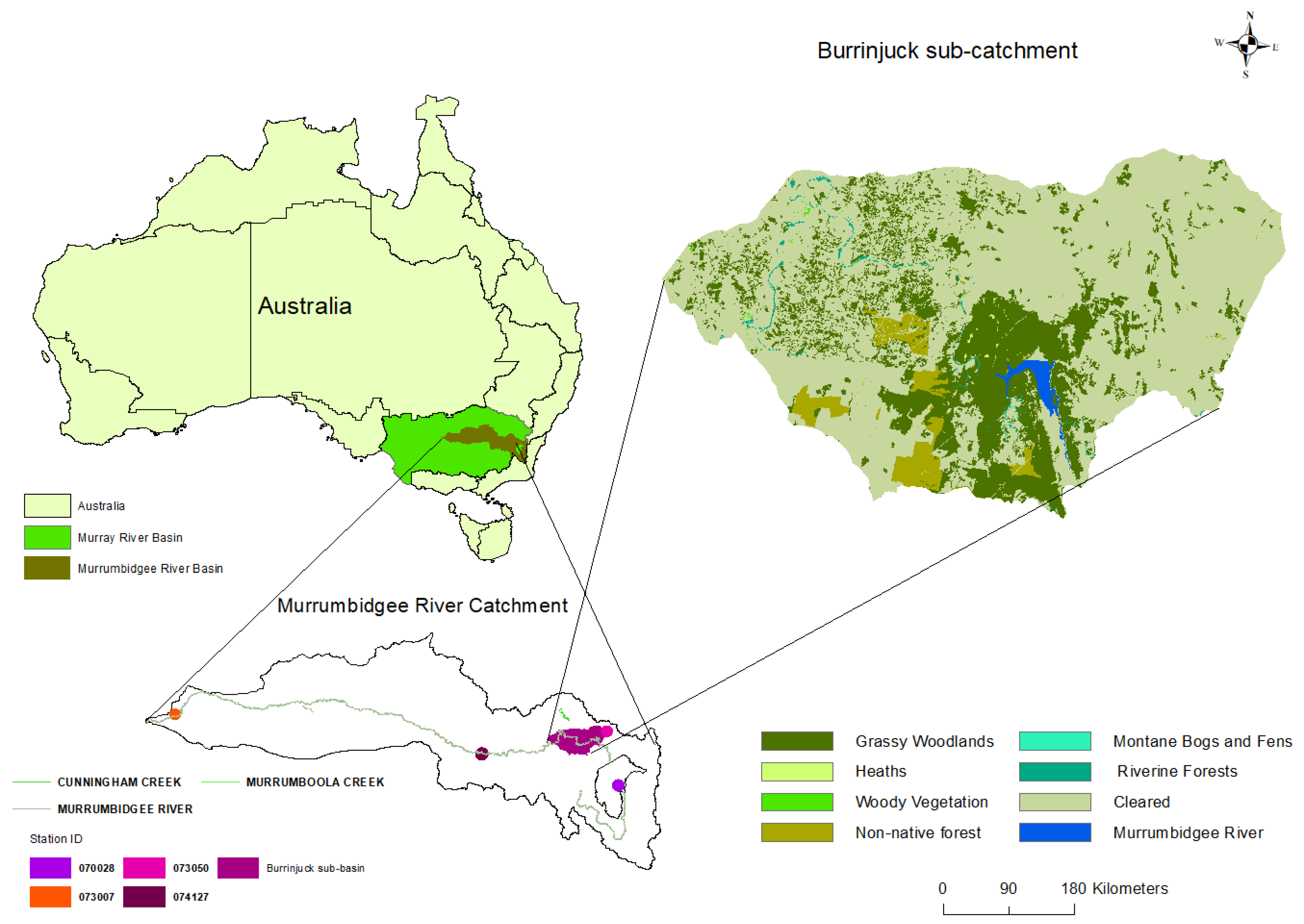
2.1. Study Area

We selected the Burrinjuck sub-catchment, which is part of the Upper Murrumbidgee River catchment in southeastern Australia (Figure 1), for this research. This area is located between 34.53°S and 148.31°E and −35.14°S and −148.55°E. The Burrinjuck Dam was built on the Murrumbidgee River in 1927 to improve agricultural irrigation in the southern part of New South Wales (NSW) [32]. The Murrumbidgee River begins its journey from Kosciuszko National Park with an altitude of 1500 m and flows around 316 km to enter the Burrinjuck Reservoir. We have considered this Burrinjuck sub-catchment as our area of interest because of plant diversity in this floodplain due to moderate slopes in its topography, where elevation varies from 370 m to 934 m [16]. The land use and land cover in this area are mostly controlled by forest and pasture; however, wheat and cereals also grow well in this area, contributing to the national agricultural production [32]. Moreover, the diverse rainfall in the lower and upper Murrumbidgee makes this floodplain healthy. Further, the climate of this area is described as temperate in the Köppen–Geiger climate classification system, in which the average temperature is 22 °C during warmer seasons [54]. Overall, the Burrinjuck sub-catchment has a diverse range of vegetation types and land use classes (Figure 1), which makes this area unique within the Murrumbidgee River catchment.

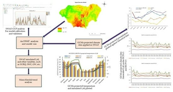
2.2. Research Methods

The research methods applied in this study have been outlined in Figure 2. The SWAT hydrological model was employed using ArcGIS (ArcMap 10.6) to mimic the Burrinjuck sub-catchment hydrology. The datasets used in this study were obtained from governmental data portals, such as Climate Change in Australia “https://www.climatechangeinaustralia.gov.au/en/ (accessed on 28 November 2022)”, the Bureau of Meteorology (BOM) “http://www.bom.gov.au (accessed on 28 November 2022)”, and the U.S. Geological Survey (USGS) “https://www.usgs.gov (accessed on 5 August 2022)”. For data analysis, Microsoft Excel (v2402) and Tableau (v2021.4) tools were used. The ArcSWAT (v2012.10.6) that simulated the LAI has been calibrated and validated against the Moderate Resolution Imaging Spectroradiometer (MODIS) LAI data. To determine the SWAT performance, the calibration and validation processes were applied using the additional SWAT Calibration and Uncertainty Programs (SWAT-CUPv5.1.6) tool with station-gauged streamflow data obtained from BoM “http://www.bom.gov.au/waterdata/ (accessed on 28 November 2022)”.

2.3. SWAT Hydrological Model

The SWAT model is a semi-distributed, physically based catchment model that continuously replicates the main water balance elements at daily or monthly time series [55]. In the SWAT model, a watershed is delineated into a number of sub-basins depending on land elevation and spatial attributes. These sub-basins are further divided into Hydrological Response Units (HRUs) according to individual land use, soil, and topography [56,57]. Each HRU is simulated for vegetation growth, soil water content, sub-surface water flow, and land management practices, in which the outputs are aggregated at the sub-basin scale through channel processes [58,59]. In this research, our primary focus is identifying vegetation growth at the HRU level. The water balance calculations at the HRU level include surface runoff, infiltration, evaporation, plant consumption, lateral flow, and percolation to sub-surface areas [56]. SWAT estimates surface runoff and infiltration from daily precipitation using the Soil Conservation Service (SCS) and Curve Number (CN) method (SCS, 1972). The hydrological cycle in the watershed can be mimicked by a SWAT simulation, where the model calculation is based on the following water balance equation [56]:

$${SW}_t={SW}_0{\sum }_{i=0}^t{\left(R_{day}-Q_{surf}-E_a-W_{seep}-Q_{gw}\right)}_i$$

(1)

where SW_t is the ultimate water content in (mm), SW₀ is the amount of water content on the first soil of the day i (mm), t is time (days), R_day is the amount of rainfall on day i (mm), Q_surf is the amount of surface runoff on specific day i (mm), E_a is the amount of evapotranspiration on day i (mm), W_seep is the amount of water percolated into the vadose zone from the soil profile on day i (mm), and Q_gw is the amount of return flow on day i (mm).

The SWAT provides three methods to calculate potential evapotranspiration (PET): Priestley–Taylor, Penman–Monteith, and Hargreaves. In this study, we used the Penman–Monteith method to calculate PET [60,61]. The Penman–Monteith equation applied in SWAT can be expressed as follows:

$$\lambda E=\frac{\mathsf{\Delta }(H_{net}-G)+{\rho }_{air}.C_p.[e_z^0-{\mathrm{e}}_{\mathrm{z}}]/r_a}{\mathsf{\Delta }+\gamma (1+\frac{r_c}{r_a})}$$

(2)

where λE is the flux density of latent heat (MJ·m⁻²·d⁻¹), E is the depth rate evaporation (mm·d⁻¹), Δ refers to the gradient of the saturation vapor pressure–temperature curve (kPa·°C⁻¹), H is the net radiation (MJ·m⁻²·d⁻¹), G is the ground heat flux density (MJ·m⁻²·d⁻¹), cp is the specific heat (MJ·kg⁻¹·°C⁻¹), ${\rho }_{air}$ refers to air density (kg·m⁻³), e_z is the water vapor pressure of air at elevation (kPa), $e_z^0$ is the saturation vapor pressure of air at elevation z (kPa), r_c is the plant canopy resistance (s·m⁻¹), γ is the psychrometric constant (kPa·°C⁻¹), and r_a is the aerodynamic resistance (s·m⁻¹). Plant growth is estimated in r_c by dividing the minimum effective stomatal resistance for a single leaf, $r_l$ (s·m⁻¹) by one-half of the LAI [62]:

$$r_c=\frac{r_l}{0.5.LAI}$$

(3)

Further details regarding the water balance and ET equations can be found in the SWAT documentation [56].

2.4. Vegetation Dynamics in SWAT Model

The SWAT model incorporates the simplified version of the Erosion Productivity Impact Calculator (EPIC) plant growth module to simulate the annual vegetation growth [56,63]. In the EPIC plant growth module, the LAI was simulated as a function of canopy height, which is required to calculate the canopy resistance and the aerodynamic resistance [56]. At the initial stage of plant growth, canopy height, and leaf area development are controlled by the optimal leaf area development function. The function of the optimal leaf area development is listed as follows [55,63]:

$${fr}_{{LAI}_{max}}=\frac{{fr}_{PHU}}{{fr}_{PHU}+\mathrm{e}\mathrm{x}\mathrm{p}({\mathrm{l}}_1-{\mathrm{l}}_2\ast {fr}_{PHU})}$$

(4)

$${fr}_{PHU}=\frac{\sum _{i=1}^{d}HU}{PHU}$$

(5)

where ${fr}_{{LAI}_{max}}$ is the fraction of the plant’s maximum leaf area index for the plant, ${\mathrm{l}}_1$ and ${\mathrm{l}}_2$ are the shape coefficients, ${fr}_{PHU}$ is the fraction of potential heat units for a certain period during the growing season, HU is the heat units accumulated on a given day (d), which can only have a positive value, and PHU is the potential heat unit required for each plant’s maturity. PHU refers to the number of days between budding and leaf senescence. For annual and perennial plant growth, before the LAI reaches its maximum value, the leaf area added on day i is calculated as follows [56]:

$$\mathrm{\Delta }{LAI}_i=\left({fr}_{{LAI}_{max,i}}-{fr}_{{LAI}_{max,i-1}}\right)\ast {LAI}_{max}\ast \{1-e^{\left[5x\right({LAI}_{i-1}-{LAI}_{max}\left)\right]}\}$$

(6)

which is then used to calculate the total leaf area index as follows [56]:

$${LAI}_i={LAI}_{i-1}+{\mathsf{\Delta }LAI}_i$$

(7)

In the above equations, $\mathsf{\Delta }{LAI}_i$ is the leaf area added on day i, ${LAI}_i$ and ${LAI}_{i-1}$ are the leaf area index on day i and the leaf area index on the previous day, ${fr}_{{LAI}_{max,i}}$ and ${fr}_{{LAI}_{max,i-1}}$ are the fraction of the plant’s maximum leaf area for day i and i − 1, respectively. ${LAI}_{max}$ is the maximum leaf area index of the plant. ${LAI}_{max}$ for a grown tree can be adjusted by multiplying the fraction of the age (growth year) of the tree and the year for the tree species to reach full growth [56]. However, the actual LAI calculated for each day may differ from optimum growth due to variations in the availability of temperature, soil water, and other factors.

By default, SWAT uses a fundamental feature named ‘dormancy’ in which plants become inactive during the days of the shortest daylight length in the year. During dormancy, a portion of biomass changes to residue, where the LAI value is minimized for related plants. Dormancy also resets a fraction of potential heat units to zero. Thus, a new growing cycle begins when the length of the day reaches the latitude-specific threshold. However, tropical plants do not become dormant, and heat units and a fraction of potential heat units accumulate continuously throughout the whole simulation period. As SWAT only simulates plant growth until the plant reaches maturity, the model configuration requires adding a ‘kill’ option to stop the growth of the plant and trigger another one. In our study, we considered the plant growing season to start from the beginning of the simulation for trees. This model setting forced SWAT to consider a starting growth cycle at the beginning year in the simulation period, which is 8 years long. In the rest of the periods, the potential heat units increased continuously because the reset mechanism was not considered without dormancy. Therefore, the LAI simulations in SWAT, based on the scheduled management operation, represent higher values in summer and lower values in winter [49]. The reliability of SWAT simulations in projecting the vegetation LAI under future climate conditions depends on the accuracy of climate projections and their spatial and temporal resolution.

2.5. Hydrological Model Setup

SWAT2012 can be run using the GIS tool in the Windows operating system. In this study, we used ArcMap v10.6 (desktop version) to execute SWAT2012 Revision 681. The watershed was outlined using a digital elevation model (DEM) with a resolution of 30 m. A total 872 km² drainage area was selected within the Burrinjuck sub-basin with the help of the DEM and the Murrumbidgee River network. Thus, it divided the watershed into 18 sub-basins and then categorized them into 158 HRUs depending on unique land use, soil, and slope. After the completion of the SWAT setup, it was initially spun up for twenty-one years from 2000 to 2020, including two years of warmup periods. The SWAT model calibration was performed against historical streamflow data using the additional SWAT Calibration and Uncertainty Programs (SWAT-CUP) tool. Moreover, the SWAT model was also calibrated using remotely sensed LAI data processed from 500 m spatial resolution and an 8-day temporal dataset of the MODIS LAI type MOD15A2H for each HRU by spatial aggregation. High-resolution climate data, satellite imagery, and ground-based observations are essential for improving the representation of vegetation characteristics in the model.

2.6. Model Performance Criteria

Hydrological model performance evaluation is crucial to assess model accuracy and reliability in simulating the behavior of the hydrological system. There are different metrics and methods for model performance evaluation. However, the selection of evaluation criteria may depend on the specific objectives of the modeling and the available data. In this study, we selected a few statistical metrics, such as the coefficient of determination (R²), Nash–Sutcliffe Efficiency (NSE), and percent bias (PBIAS) quantitative statistics [64,65,66]. Furthermore, we utilized twenty-one SWAT parameters in the SWAT-CUP simulation and organized them based on the model performance acceptance guidelines proposed by Arnold et al. [58], which are explained in the following section.

The NSE, also known as the Nash–Sutcliffe coefficient, is a widely used dimensionless statistical metric to assess the performance of hydrological models or other environmental models. The NSE is particularly useful for evaluating models that simulate time series data, such as streamflow or water level. The NSE compares the predictive performance of a model with the performance of a simple benchmark model, usually represented by the mean of the observed data. The NSE ranges from negative infinity to 1, with 1 representing a perfect match between the predicted and the observed data, 0 indicating that the model performs no better than the mean of the observed data, and negative values indicating that the model performs worse than the mean. The NSE is defined as follows [67]:

$$NSE=1-\frac{\sum _{i=1}^n{\left(Q_{obs},i-Q_{sim},i\right)}^2}{{\sum }_{i=1}^n{\left(Q_{obs},i-\overline{Q_{obs}}\right)}^2}$$

(8)

In the above equation, n is the number of time steps, $Q_{obs}$, i is the observed flow at time step i (daily here), $Q_{obs}$ is the mean of the observed flow, and $Q_{sim}$, i is the simulated flow.

The coefficient of determination, known as R² (R-squared), is a statistical metric used to assess how well a regression model fits the observed data. In the context of regression analysis, R² quantifies the proportion of the variance in the dependent variable that is predictable from the independent variable(s) in the model. It provides a statistical measure of the goodness-of-fit of the regression model. The R² value ranges from 0 to 1, where 0 indicates that the regression model explains none of the variance in the dependent variable, meaning it does not fit the data at all. A water balance model is deemed successful when it achieves a higher coefficient of determination R², indicating a more favorable outcome [68]. R² is defined as follows [68,69]:

$$R^2={\{\frac{{\sum }_{i=1}^n(Q_i^{obs}-{\overline{Q}}^{sim})(Q_i^{sim}-{\overline{Q}}^{sim})}{{{\sum }_{i=1}^n(Q_i^{obs}-{\overline{Q}}^{obs})}^2{{\sum }_{i=1}^n(Q_i^{obs}-{\overline{Q}}^{obs})}^2}\}}^2$$

(9)

where, $Q_i^{obs}$ and $Q_i^{sim}$ are representing the measured and simulated data for the ith observation and ${\overline{Q}}^{obs}$ and ${\overline{Q}}^{sim}$ are the mean of the measured and simulated data, respectively.

The percent bias (PBIAS) quantifies the systematic inclination of the model toward either overestimating or underestimating simulated values compared to the observed data [58]. The PBIAS value reaching zero signifies that the simulation is impartial and closely resembles the observed data. Typically, a lower PBIAS value indicates a more precise model simulation overall. PBIAS is calculated as follows [70]:

$$PBIAS=\frac{{\sum }_{i=1}^n\left(Q_i^{obs}-Q_i^{sim}\right)\ast 100}{{\sum }_{i=1}^n{Q}_i^{obs}}$$

(10)

In the above equation, $Q_i^{obs}$ and $Q_i^{sim}$ express the observed and simulated data for the ith observation, respectively.

2.7. Trend Analysis

In this research, we applied the Mann–Kendall test, a non-parametric statistical test commonly known as the Mann–Kendall trend test, to assess the existence or absence of a monotonic trend in time series data. This test is particularly useful when the traditional parametric test is less appropriate or the time series data do not meet the normal assumptions. This Mann–Kendall test is commonly used in different research studies, including earth science, hydrology, climatology, etc., to understand whether there is a significant increasing or decreasing trend, as well as to quantify the strength of that trend. The following Equation (11) is used to determine the Mann–Kendall test statistic [71].

$$S={\sum }_{i=1}^{n-1}\ast {\sum }_{j=i+1}^{n}sign(X_j-X_i)$$

(11)

where $X_j$ and $X_i$ represent sequential data in the time series, and n represents the size of the time series. In the above equation, j > i and i = 1, 2, 3… n − 1, k = 2, 3, 4… n. The $sign(X_j-X_i)$ is calculated using Equation (12)

$$sign(X_j-X_i)=\left\{\begin{array}{c}+1 if(X_j-X_i)>0\\ 0 if(X_j-X_i)=0\\ -1 if(X_j-X_i)<0\end{array}\right.$$

(12)

The variance of S can be calculated from the following equation [71]:

$$Var(S)=\frac{S(n-1)(2n+5)-{\sum }_q^p{t}_p(t_p-1)(2t_p+5)}{18}$$

(13)

where q is the number of tied groups in the datasets, $t_p$ is the number of data in the pth tied group, and n is the total number of data in the time series. A positive value of S indicates that an increasing and negative value of S is a decreasing trend of time series data. The following Equation (14) is used to calculate the standard test statistics [71].

$$Z_s=\left\{\begin{array}{c}\frac{S-1}{\sqrt{var\left(S\right)}} if S>0\\ 0 if S=0\\ \frac{S+1}{\sqrt{var\left(S\right)}} if S<0\end{array}\right.$$

(14)

The degree or rate of change can be calculated using the Thiel-Son slope method. Equation (15) is used to calculate the Theil–Sen slope (β) [72,73].

$$\beta =median\left(\frac{{\mathrm{X}}_{\mathrm{j}}–{\mathrm{X}}_{\mathrm{i}}}{j-i}\right)$$

(15)

where $X_j$ and $X_i$ represent sequential data in the time series, i = 1, 2, 3… n − 1 and j > i.

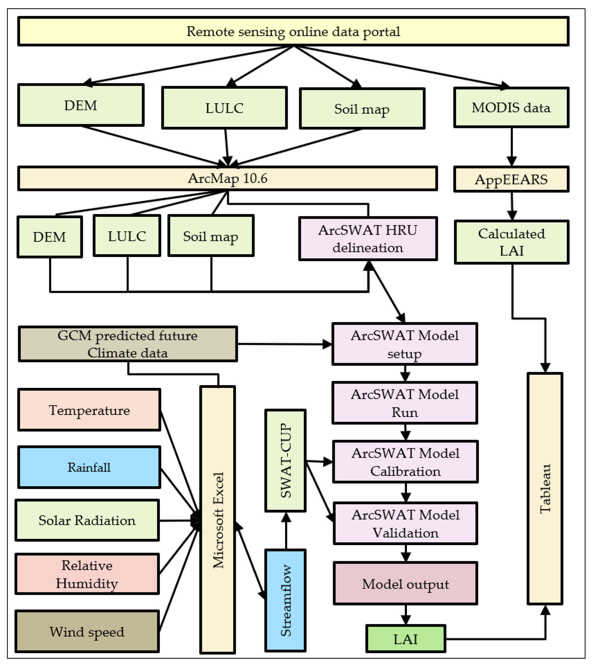
2.8. Data Preparation

SWAT requires a combination of both climate and land properties data to build a hydrological model. These data requirements can be categorized into essential, such as DEM, soil map, land use map, and weather data (precipitation, temperature, windspeed, solar radiation, and relative humidity), and non-essential, such as streamflow, reservoir information, sediment transfer, water quality, chemical, and pesticide data. The datasets used in this study, including their source of availability, are listed in

Table 1. The data used in this study include the frequency, source, and description.

Data	Frequency	Description	Source
DEM	-	30 m spatial resolution	USGS
Land cover/land use map	-	50 m spatial resolution	NSW Office of Environment and Heritage
Soil Map	-	250 m spatial resolution	Digital Atlas of Australian Soil
MODIS LAI	8-Day	500 m spatial resolution	USGS
Temperature	Daily	Station gauged, temporal	BoM
Solar Radiation	Daily	Station gauged, temporal	BoM
Precipitation	Daily	Station gauged, temporal	BoM
Relative humidity	Daily	Station gauged, temporal	BoM
Wind speed	Daily	Station gauged, temporal	BoM
Streamflow (discharge)	Daily	Station gauged, temporal	NSW Office of Water

. A detailed description of SWAT input data was outlined by Muhury et al. [16].

2.9. Leaf Area Index (LAI)

The LAI is widely used in research studies to assess the amount of leaf area in an ecosystem, which is a dimensionless and time-dependent vegetation parameter [74]. Watson [75] defined the LAI as the ratio of one-sided leaf area in the canopy per unit ground surface area [m² m⁻²]. It exhibits dynamism and is susceptible to variations influenced by internal and external factors, including plant type, orientation, seasonality, nutrition availability, and diseases [43]. Processes within ecosystems heavily depend on the LAI as a pivotal factor, encompassing functions like respiration, rainfall interception, transpiration (ET), and biophysical cycles. Therefore, vegetation growth, yield, biomass, energy, and water balances in ecosystems have been extensively assessed through the widespread application of the LAI in agricultural and forestry research. For broad-leaf plants, LAI = leaf area/ground area, m²/m², has a value range from 0 to 10 depending on plant physiology and growth phase [76].

2.10. Global Climate Models (GCMs)

Global climate models (GCMs) serve as essential instruments for evaluating climate change and producing projections of future climatic conditions [14]. The Coupled Model Intercomparison Project 5 (CMIP5) has presented a variety of sophisticated Global Climate Models (GCMs) that have incorporated carbon cycle models and a dynamic vegetation model [77]. Australian Government Climate Agencies have recognized eight of these General Circulation Models (GCMs) as exhibiting the highest performance. For future climate projections in this study, we examined two climate scenarios, RCP 4.5 and RCP 8.5. The RCP 4.5 represents a scenario of medium-low stabilization, wherein radiative forcing reaches a state of stability at 4.5 Wm² by the year 2100 with 650 ppm CO₂ concentration [32]. However, RCP 8.5 depicts an exceptionally elevated emission scenario, signifying a pathway characterized by high radiative forcing to 8.5 Wm² by the year 2100 with CO₂ concentration. After conducting a robust literature review, the outputs of three GCMs, i.e., ACCESS1.0, MK3.6, and MIROC5, were used to assess the future climate change impact on the Burrinjuck sub-basin vegetation community. ACCESS1.0, MK3.6, and MIROC5 were selected to project future climate variables such as temperature and precipitation that directly correlate to vegetation growth for the two emission scenarios RCP 4.5 and RCP 8.5. Nevertheless, the ACCESS1.0 climate model (known as the maximum consensus scenario model), characterized as the prospective climate generated by the largest proportion of models, requires a quantity exceeding one-third of the total available GCMs [32].

2.11. Climate Scenarios

This study evaluates the projections of GCMs for two climate scenarios across upcoming time periods, i.e., (i) 2031–2055, (ii) 2056–2075, and (iii) 2076–2100. The scenarios are established by examining daily time series of projected climate data, spanning from 2031 to 2100, encompassing variables such as rainfall, temperature, wind speed, solar radiation, and relative humidity. Scenario 1: RCP 4.5 projections for 2031–2055, 2056–2075, 2076–2100. Scenario 2: RCP 8.5 projections for 2031–2055, 2056–2075, 2076–2100.

Figure 3a shows the average maximum temperatures, according to the ACCESS1.0 model, which are close to the historical maximum temperature under RCP 4.5. However, the minimum temperatures are slightly above the average historical minimum temperature shown in Figure 3d. According to MIROC5 and MK3.6 climate model projections, the average maximum temperature from January to May decreases, and from June to December, the maximum temperature shows an increasing trend (Figure 3b,c). These two climate models predicted minimum temperature decreases from January to June and increases from July to December over three projected time periods according to RCP 4.5 climate scenarios (Figure 3e,f).

In contrast to climate scenario 8.5, the ACCESS1.0 GCM predictions show that the average maximum and minimum temperatures will be increased compared to the historical averages when considering the future time frames (Figure 4a,d). Likewise, both MIROC5 and MK3.6 predict that the average maximum temperatures from January to June are below the historical average maximum and that the average temperatures from July to December are above the historical average (Figure 4b,c). However, the average minimum temperatures under MIROC5 for the first five months of the year are close to the historical average minimum, whereas the rest of the month’s average is higher than the historical average minimum temperature (Figure 4e). Considering the MK3.6, January to May temperature projections are below the historical average, and July to December predictions are above the historical average temperature (Figure 4f).

3. Results

3.1. Analysis of the SWAT Model Output and Parameter Sensitivity

In this study, a SWAT model was built using ArcGIS interface (ArcSWAT) in the study area based on remote sensing data, high-resolution DEM, soil map, and LULC map. A pre-calibration parameter selection was made according to a previous SWAT model run for hydrological and vegetation analysis. The model was initially run with monthly historical climate data from 2000 to 2020, which covers both drought and flood conditions in the study area.

Table 2. Performance indices of SWAT model parameters.

Parameter Name	Description	t-Stat	p-Value	Sensitivity Rank
CH_N1.sub	Channel Manning’s n	3.03	0.06	1
SOL_AWC.sol	Available water capacity in the soil	−2.68	0.08	2
ESCO.hru	Soil evaporation compensation factor	2.02	0.14	3
GW_REVAP.gw	Groundwater revap coefficient	−1.89	0.16	4
REVAPMN.gw	Threshold depth of water in the shallow aquifer for revap to occur [mm]	1.67	0.19	5
CH_K2.rte	Hydraulic conductivity of the channel [mm/hr]	1.61	0.21	6
CN2.mgt	Curve Number	−1.58	0.21	7
SURLAG.bsn	Surface runoff lag coefficient	1.45	0.24	8
CANMX.hru	Maximum canopy storage [mm]	1.39	0.26	9
HRU_SLP.hru	Average slope steepness [m/m]	1.29	0.29	10
SOL_Z.sol	Depth of the soil layer [mm]	−1.12	0.34	11
SLSUBBSN.hru	Average slope length [m]	−1.11	0.35	12
SLSOIL	Slope length for lateral subsurface flow	−1.10	0.35	13
ALPHA_BNK.rte	Baseflow alpha factor for bank storage (day−1)	1.06	0.37	14
ALPHA_BF.gw	Base flow alpha factor (day−1)	1.06	0.37	15
EPCO.hru	Plant uptake compensation factor	0.87	0.45	16
RCHRG_DP.gw	Deep aquifer percolation fraction [fraction]	−0.83	0.47	17
SOL_K(..).sol	Saturated hydraulic conductivity of the soil [mm/hr]	−0.78	0.49	18
GWQMN.gw	Threshold depth of water in the shallow aquifer required for return flow to occur [mm]	0.75	0.51	19
GW_DELAY.gw	Groundwater delay [days]	−0.23	0.83	20
CH_N2.rte	Manning’s coefficient of the channel	0.02	0.98	21

lists the sensitivity ranking of the twenty-one parameters. The top five parameters according to the list were CH_N1, SOL_AWC, ESCO, GW_REVAP, and REVAPMN (Table 2).

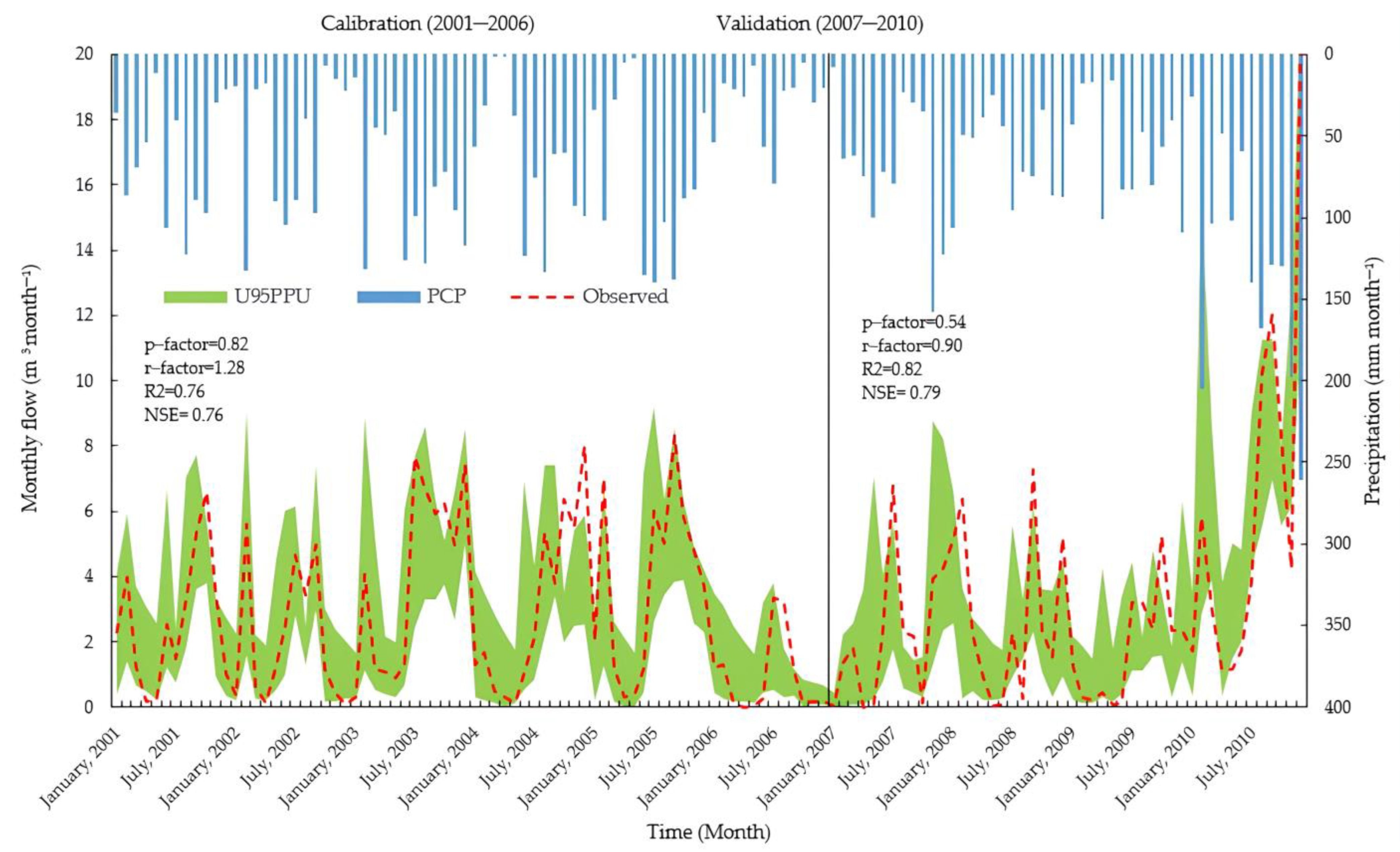
3.2. Analysis of the SWAT Model Calibration and Validation against Streamflow

The parameters from the sensitivity analysis have been applied for model validation. The calibration and validation results have been analyzed to assess the model performance, which produced 0.79 and 0.67 NSE values for the calibration and validation, respectively. The performance parameters for the SWAT model developed in the study area can be identified as ‘good’. Based on the result, the model within the study area successfully replicated approximately 79% of the variability observed in streamflow data. Moreover, ‘R’ values confirm a good correlation between observed and simulated streamflow during calibration and an acceptable correlation for validation. The ‘R’ values for the calibration show very good performance (R = 0.82) and satisfactory (R = 0.67) for validation. Furthermore, the SWAT model exhibited a significant improvement in statistical indices. Figure 5 shows calibration and validation results from SUFI-2 comparing observed and simulated streamflow from 2002 to 2006 and 2007 to 2010, respectively. These results confirm that the SWAT model was able to simulate streamflow relatively close to the observed values, which is a fundamental criterion for SWAT watershed applications [49,78]. The hydrographs indicate a noticeable disparity between the observed and simulated values in the plots. Additionally, the model slightly overestimated the low flow throughout both the calibration and validation periods.

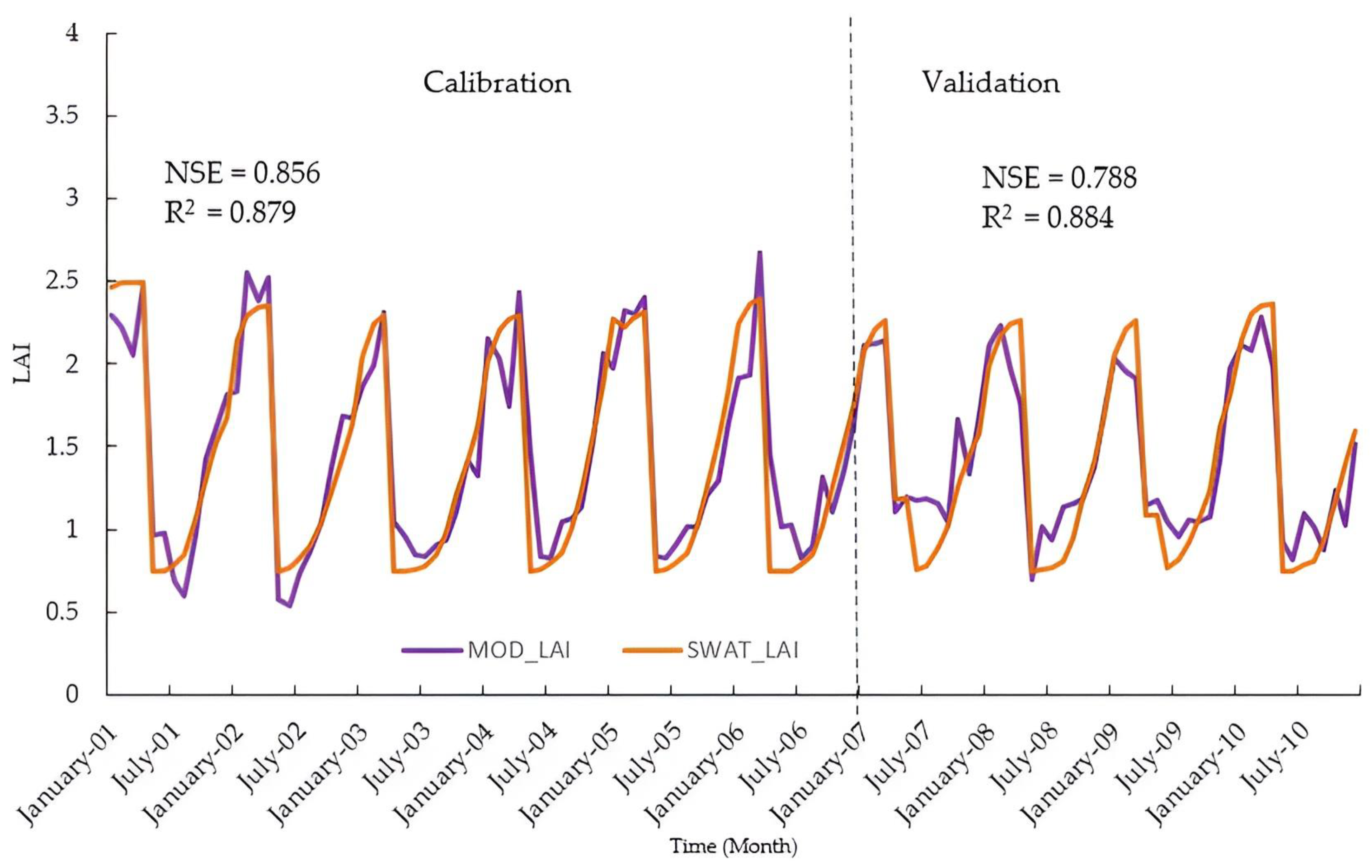
3.3. Analysis of the SWAT Model Calibration and Validation against MODIS LAI

In this study, we performed manual calibration between the SWAT-simulated LAI and MODIS LAI. We downscaled the MODIS LAI to match the basic calculation units of the SWAT model. The linear interpolation method was applied to segregate the 8-day MODIS LAI data into daily time series data and then aggregated to monthly data. The monthly average LAI for the entire watershed was determined using both downscaled and original MODIS LAI datasets. The seasonal patterns of variation were consistent between the two datasets, with the highest LAI available in December and January and the lowest values observed in June. In December, the LAI reaches its peak value for the original SWAT model. In almost every month, the original SWAT simulated value was noticeably higher than the remotely sensed LAI. Figure 6 represents the calibration and validation results between the SWAT LAI and MODIS LAI for ten years from 2001 to 2010. Validation of the model against independent datasets is crucial for assessing its reliability in capturing spatial and temporal variations in LAI.

3.4. The Outcomes of the Trend Analysis of the Precipitation (Observed and Projected)

In this study, a Python script was created to calculate a non-parametric Mann–Kendall trend test and Sen’s slope to identify the trends and quantify the change for GCMs projected future rainfall at the Burrinjuck sub-catchment. The trend analysis was consolidated into baseline (1980–2020), near future (2031–2055), mid-century (2056–2075) and late-century (2076–2100) periods.

Table 3. Trend analysis of the historical (1980–2020) and three GCM’s predicted rainfall for future period (2031–2055).

Model	Scenarios	Annual			Summer			Autumn			Winter			Spring
		p	Zs	β	p	Zs	β	p	Zs	β	p	Zs	β	p	Zs	β
Historical	Baseline	0.098	−1.65	−5.94	0.451	0.75	0.35	0.645	−0.46	−0.185	0.0172	−2.381	−1.089	0.597	−0.527	−0.288
ACCESS1.0	RCP 4.5	0.194	−1.297	−1.326	0.440	−0.770	−0.175	0.050	−1.956	−0.164	0.251	1.145	0.135	0.282	−1.074	−0.188
ACCESS1.0	RCP 8.5	0.0491	−1.967	−1.777	0.795	−0.258	−0.0527	0.152	−1.429	−0.137	0.516	−0.648	−0.080	0.0515	−1.946	−0.255
MIROC5	RCP 4.5	0.737	−0.334	−0.482	0.090	−1.693	−0.334	0.298	1.039	0.137	0.594	0.532	0.100	0.715	0.365	0.067
MIROC5	RCP 8.5	0.116	1.571	2.203	0.605	0.517	0.095	0.114	1.576	0.192	0.167	1.378	0.196	0.437	0.775	0.185
MK3	RCP 4.5	0.130	−1.510	−1.128	0.411	−0.821	−0.116	0.155	−1.419	−0.081	0.026	−2.225	−0.111	0.405	−0.831	−0.102
MK3	RCP 8.5	0.011	−2.51	−1.350	0.863	0.172	0.016	0.014	−2.453	−0.157	0.0001	−3.761	−0.189	0.293	−1.049	−0.101

p-value (p) is a statistical measure; Z-score (Zs) is a standardized score; β (beta) represents the slope coefficient. The bold numbers are accepted values in the trend analysis.

shows that the annual rainfall decreases by 1.96 mm and 2.51 mm according to the ACCESS1.0 and MK3.6 model projections under the RCP 8.5 climate scenario. Moreover, according to MK3.6, the autumn and winter rainfall would also decrease significantly by 2.45 mm and 3.76 mm, respectively, under the same climate scenario. However, the MIROC5 projection shows that the rainfall would increase during autumn, winter, and spring under RCP 4.5 and RCP 8.5 climate scenarios.

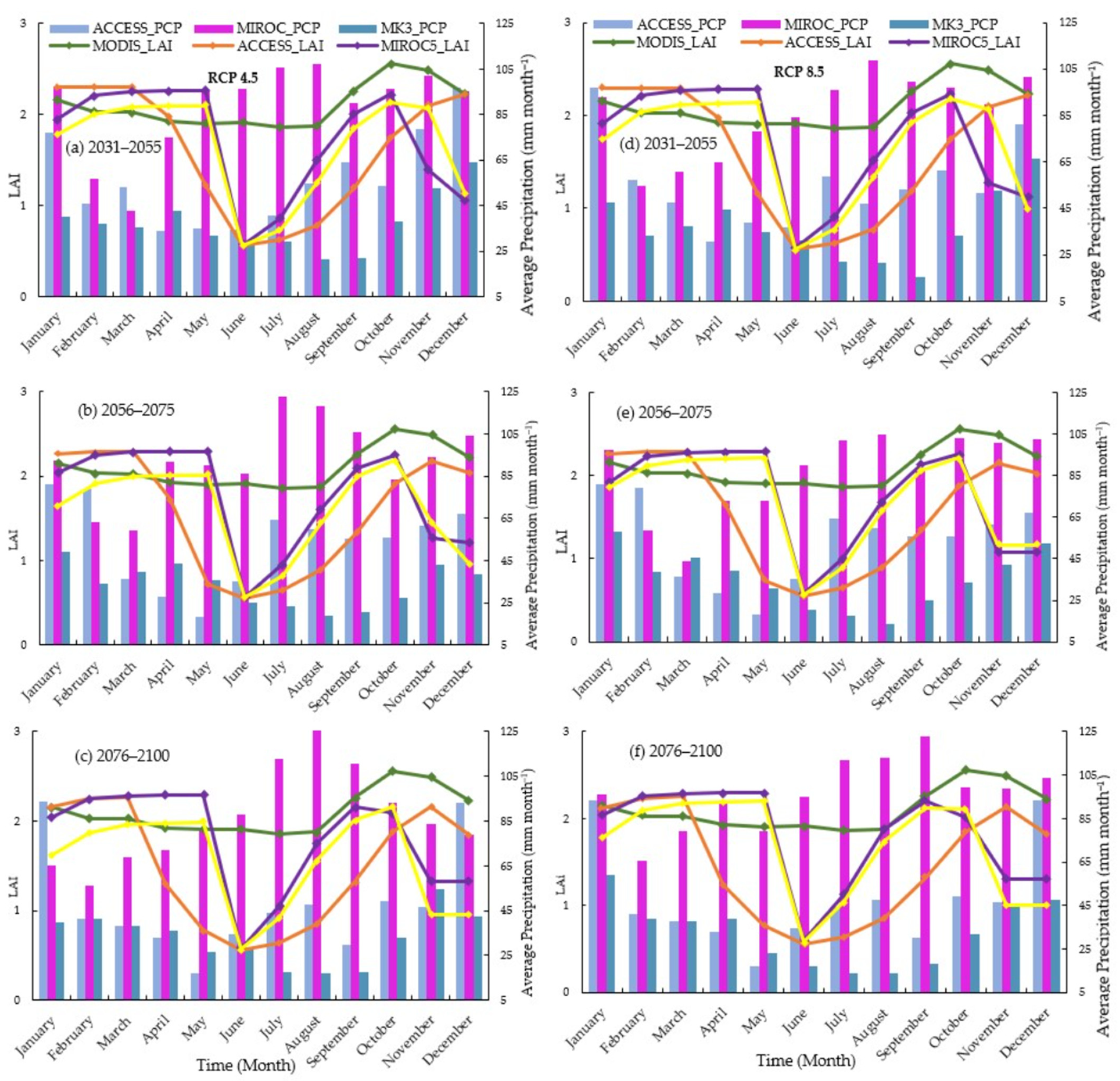
3.5. Analytical Results of LAI Responses to the Future Precipitation Changes

Precipitation is another important climate variable that makes water available in the soil as soil water content for vegetation growth. To visualize the impacts of the precipitation, we plotted the average monthly precipitation against the SWAT simulated the LAI in three different future time frames (Figure 7). The plotted result shows that winter and spring rainfall has positive impacts on the LAI for all GCMs under both climate scenarios. However, the LAI shows a slight increase in lateral movement during summer and autumn, where average rainfall is below 45 mm. Moreover, the simulated LAI for all GCMs under both scenarios, from February to April, is higher than the MODIS LAI in all three projected time frames (Figure 7).

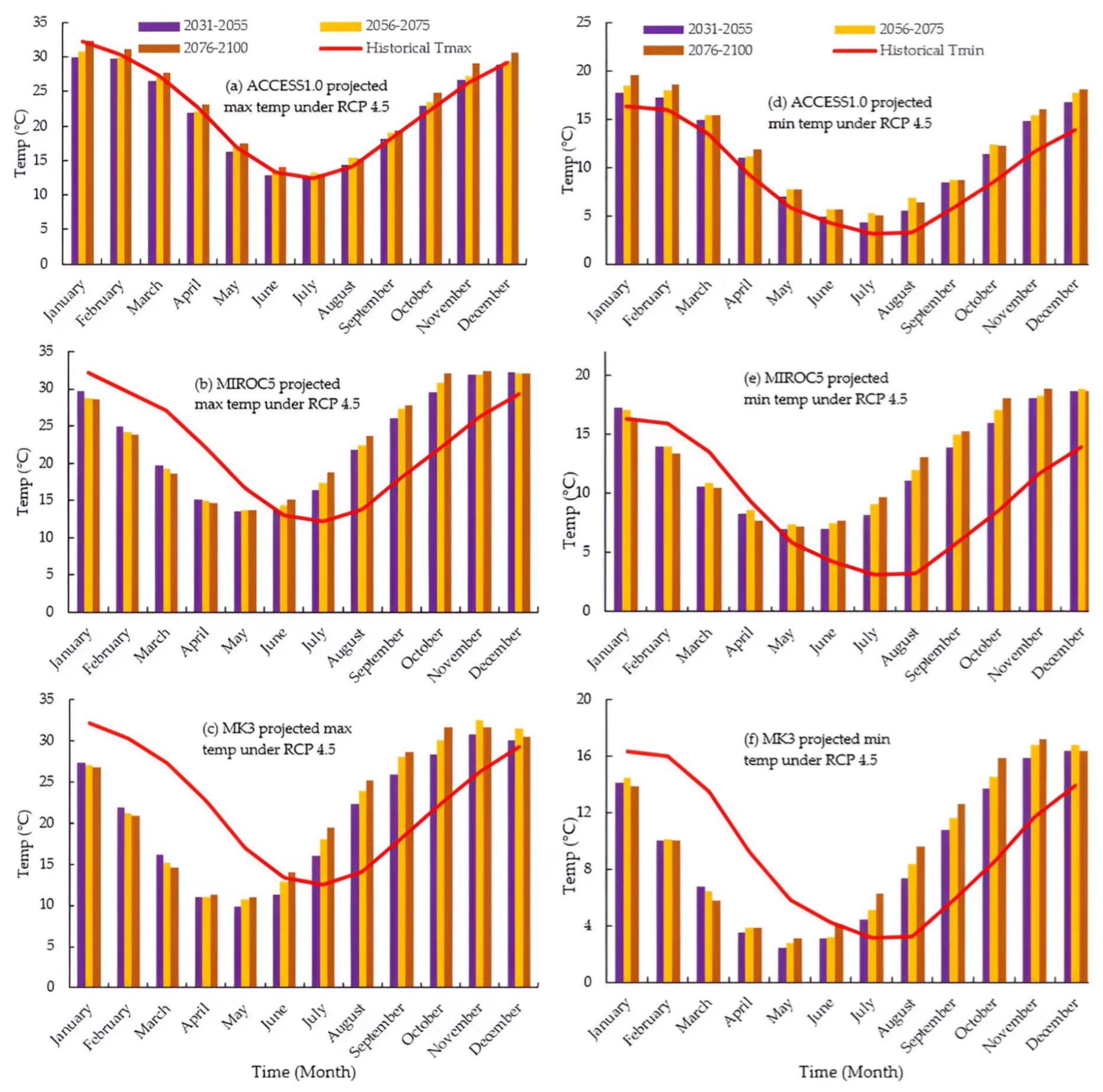
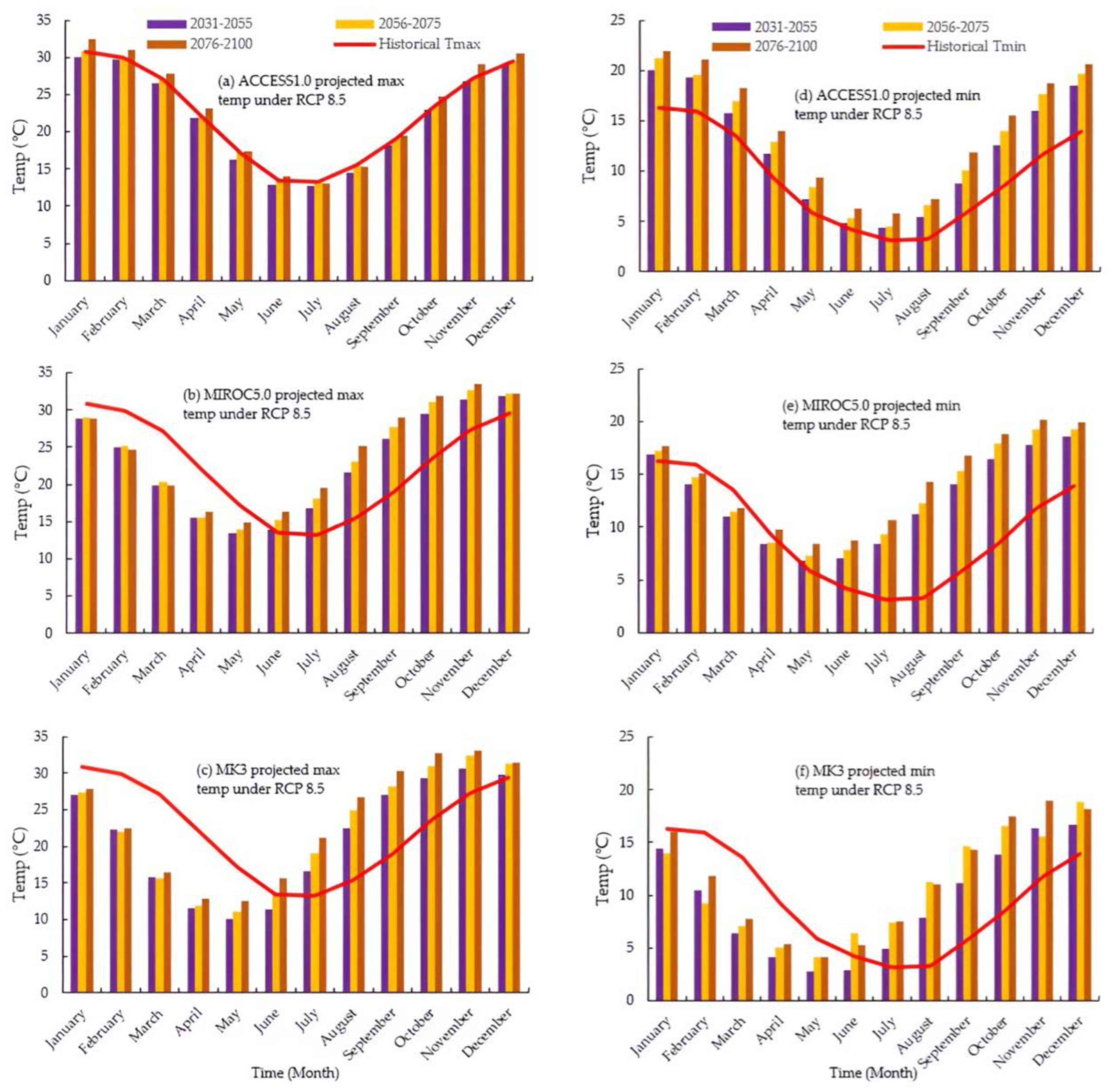
3.6. Analytical Results of LAI Responses to Future Temperature Changes

To understand how vegetation responds to forthcoming climate factors, we examined the SWAT-simulated LAI data in comparison with temperatures projected by GCMs (Figure 8). Considering ACCESS1.0 GCM projections, the simulated LAI decreases along with temperature decrease from January to June in the future time frames under climate scenario RCP 4.5 and RCP 8.5. However, the LAI increases from July to December when the temperature also increases in the study area for the same scenario (Figure 8). Further, the simulated LAI, using MIROC5 and MK3.6 climate data, presents a positive increase from June to October and then decreases until December under both climate scenarios and for all future time frames (Figure 8).

The SWAT simulated LAI data were analyzed under two different climate scenarios, RCP 4.5 and RCP 8.5, against the MODIS LAI. In this analysis, we have considered the average MODIS LAI data from 2001 to 2020 as a benchmark to quantify future LAI changes. The SWAT simulated LAI mostly shows a decrease in all time frames except January to April in 2031–2055, January to March in 2056–2075, and February to March in 2076–2100, according to ACCESS1.0. The highest 10.86% LAI increase was noticed according to ACCESS1.0 during the period of 2031–2055 (

Table 4. SWAT simulated LAI changes (percent of change compared to MODIS LAI data) listed against changes in predicted temperature (TMP). The SWAT model was prepared using the GCM’s predicted climate data input under the RCP 4.5 climate scenario.

RCP 4.5	ACCESS1.0						MIROC5						MK3.6
	2031–2055		2056–2075		2076–2100		2031–2055		2056–2075		2076–2100		2031–2055		2056–2075		2076–2100
Month	TMP	LAI	TMP	LAI	TMP	LAI	TMP	LAI	TMP	LAI	TMP	LAI	TMP	LAI	TMP	LAI	TMP	LAI
Jan	−2.33	5.75	−4.24	4.28	0.65	−0.01	−7.60	−9.70	−10.60	−5.03	−11.40	−5.26	−15.18	−18.63	−5.09	−27.36	−16.83	−29.96
Feb	1.28	10.72	1.07	10.23	5.05	8.79	−15.65	7.30	−18.46	9.02	−19.47	8.91	−26.12	−1.17	−8.39	−5.46	−29.41	−7.67
Mar	−2.03	10.86	0.39	10.56	2.79	9.74	−27.36	9.04	−28.64	10.30	−30.93	10.23	−40.43	2.35	−11.88	−1.66	−46.10	−3.25
Apr	−1.24	2.57	−0.20	−10.34	4.76	−41.26	−31.70	13.67	−32.17	14.69	−34.01	14.63	−50.34	7.38	−11.16	3.71	−48.69	2.47
May	1.60	−47.44	3.49	−127.57	5.00	−115.24	−18.57	14.59	−17.10	15.51	−17.73	15.47	−40.71	8.40	−5.92	4.93	−33.47	3.92
Jun	1.73	−179.24	3.73	−178.90	7.87	−178.40	5.44	−175.74	10.02	−173.46	16.53	−171.00	−12.70	−178.49	−0.10	−176.18	7.40	−175.25
Jul	2.18	−151.22	8.66	−141.16	6.99	−145.16	34.30	−93.97	43.01	−78.61	54.53	−65.92	31.36	−123.07	5.93	−102.43	59.80	−84.43
Aug	10.73	−112.95	11.86	−90.35	10.77	−97.87	57.91	−22.07	62.49	−14.96	71.83	−6.50	61.40	−43.48	10.07	−26.69	82.10	−18.03
Sep	4.09	−77.03	5.15	−59.58	7.63	−61.46	44.10	−11.59	51.63	−7.21	54.02	−4.39	43.37	−20.21	10.06	−11.80	58.29	−11.41
Oct	5.82	−41.77	6.55	−30.85	12.69	−32.69	33.91	−14.15	39.68	−12.92	45.29	−20.59	28.64	−18.15	8.01	−15.56	43.44	−17.28
Nov	8.71	−16.91	4.08	−13.08	10.81	−13.91	21.93	−68.93	21.73	−82.67	23.51	−76.21	17.34	−18.62	6.21	−62.77	20.49	−131.88
Dec	2.63	−0.28	0.69	−8.44	4.48	−18.89	10.24	−92.64	9.60	−71.44	9.65	−59.11	2.90	−81.69	2.22	−108.62	4.13	−109.38

).

In contrast to the RCP 8.5, the simulated LAI using MIROC5 and MK3.6 data shows a downward trend starting in June. Moreover, a significant decrease was found in June, by 179.24%, 175.74%, and 178.85%, respectively, according to all three GCMs. Likewise, a decrease in LAI continues until December. However, there is an increasing trend in LAI from February to May under the MIROC5 and MK3.6 projections (

Table 5. SWAT simulated LAI changes (percent of change compared to MODIS LAI data) listed against changes in predicted temperature (TMP). The SWAT model was prepared using the GCM’s predicted climate data input under the RCP 8.5 climate scenario.

RCP 8.5	ACCESS1.0						MIROC5						MK3.6
	2031–2055		2056–2075		2076–2100		2031–2055		2056–2075		2076–2100		2031–2055		2056–2075		2076–2100
Month	TMP	LAI	TMP	LAI	TMP	LAI	TMP	LAI	TMP	LAI	TMP	LAI	TMP	LAI	TMP	LAI	TMP	LAI
Jan	−2.33	5.74	2.58	4.17	4.27	−1.66	−10.41	−11.61	−10.17	−11.15	−10.27	−4.85	−15.87	−21.39	−15.12	−13.88	−13.43	−19.01
Feb	1.28	10.72	4.92	10.19	11.92	8.22	−15.72	7.53	−14.72	8.04	−16.74	9.22	−24.51	0.26	−25.45	3.93	−24.11	2.69
Mar	−2.03	10.86	3.11	10.54	11.37	9.40	−26.83	9.74	−24.58	10.01	−26.53	10.46	−41.82	3.91	−42.13	6.78	−39.32	6.00
Apr	−1.24	2.57	5.89	−14.64	12.94	−48.29	−30.14	14.34	−29.54	14.52	−26.13	14.82	−47.69	9.02	−46.11	11.76	−41.52	11.14
May	1.60	−55.05	10.87	−123.86	21.65	−116.21	−19.24	15.20	−16.20	15.35	−10.17	15.62	−38.84	9.98	−33.55	12.74	−24.44	12.23
Jun	1.73	−179.24	14.60	−178.90	25.94	−178.40	7.03	−173.63	17.18	−170.02	24.93	−167.60	−12.14	−178.68	3.22	−175.93	19.64	−172.07
Jul	2.18	−151.22	17.47	−141.15	31.44	−145.16	38.47	−87.49	49.00	−71.39	61.35	−55.10	36.93	−112.26	56.50	−88.20	74.38	−66.14
Aug	10.73	−112.95	13.96	−90.34	28.94	−97.87	56.42	−20.58	67.21	−10.00	82.13	0.09	63.34	−35.35	80.62	−17.25	93.74	−7.42
Sep	4.09	−77.03	12.05	−59.77	26.94	−61.56	44.39	−10.66	53.47	−5.29	60.67	−2.14	49.85	−15.57	56.13	−8.82	67.78	−6.06
Oct	5.82	−42.05	11.12	−32.80	26.21	−34.91	33.46	−13.80	41.33	−12.54	44.87	−24.83	32.93	−16.03	40.77	−14.49	48.36	−19.93
Nov	8.71	−17.18	8.99	−14.26	21.70	−15.38	19.93	−82.56	24.39	−109.87	27.81	−78.43	16.89	−18.61	23.94	−96.43	25.89	−123.44
Dec	2.63	−0.38	8.45	−9.04	11.85	−19.91	8.82	−83.63	10.16	−89.50	10.17	−61.12	2.05	−102.91	7.18	−77.38	7.68	−101.76

).

3.7. Analytical Results of Trend Analysis of LAI in the Watershed (Observed and Simulated)

We have calculated the Mann–Kendall trend test and Sen’s slope to discover the trends in the SWAT simulated LAI for future time frames under two climate scenarios, RCP 4.5 and RCP 8.5. In this calculation, we considered the MODIS LAI data from 2002 to 2020 as baseline and two climate scenarios for three climate models which are outlined in

Table 6. Trend analysis of the MODIS LAI (2002–2020) and the three GCM’s predicted climate variables induced SWAT simulated LAI for the future time frame (2031–2055).

Model	Scenarios	Annual			Summer			Autumn			Winter			Spring
		p	Zs	β	p	Zs	β	p	Zs	β	p	Zs	β	p	Zs	β
MODIS	Baseline	0.888	−0.139	−0.0005	0.004	−2.868	−0.009	0.833	0.209	0.008	0.420	−0.805	−0.0008	0.045	−1.995	−0.005
ACCESS1.0	RCP 4.5	0.17	−1.35	−0.005	0.070	−1.805	−0.004	0.128	−1.518	−0.013	0.906	0.117	0.0	0.261	−1.123	−0.002
ACCESS1.0	RCP 8.5	0.350	−0.934	−0.004	0.083	−1.728	−0.003	0.233	−1.191	−0.007	0.888	0.140	0.0002	0.981	0.023	6.666
MIROC5	RCP 4.5	0.029	−2.175	−0.007	0.052	−1.938	−0.015	0.015	−2.416	−0.001	0.045	1.996	0.002	0.029	−2.175	−0.012
MIROC5	RCP 8.5	0.907	0.116	0.0003	0.925	0.093	0.0007	0.522	0.638	7.291	0.009	2.593	0.004	0.797	−0.256	−0.001
MK3	RCP 4.5	0.440	−0.770	−0.003	0.833	0.210	0.003	0.725	−0.350	−0.001	0.020	2.312	0.003	0.001	−3.177	−0.007
MK3	RCP 8.5	0.605	0.516	0.001	0.386	0.865	0.005	0.637	0.471	0.0013	0.035	2.097	0.002	0.021	−2.297	−0.004

p-value (p) is a statistical measure; Z-score (Zs) is a standardized score; β (beta) represents the slope coefficient.

. In this analysis, we accepted the LAI values with a p-value of less than 0.05. The analysis shows a decreasing trend for the MODIS LAI in the summer and spring by 2.86 and 1.99, respectively. Similarly, according to the MIROC5, the simulated LAI increases in winter by 1.99 and 2.59 under RCP 4.5 and RCP 8.5, respectively. However, the LAI decreases by 2.175 and 2.416 in spring and autumn, respectively, under RCP 4.5. Similarly, the MK3 model data simulated LAI increases by 2.31 and 2.09 in winter under RCP 4.5 and RCP 8.5, respectively. However, the result also shows the LAI decreases during spring by 3.17 and 2.29 according to MK3.6 under RCP 4.5 and RCP 8.5, respectively.

3.8. Analysis of the Floodplain Vegetation Responses to the SWAT Variables

In this study, we analyzed the responses of vegetation to SWAT simulated variables using LAI changes (%) in relation to soil water content (SW), surface water flow (SURQ), and groundwater flow (GW). The LAI increases from 0.16% to 58.13% by ACCESS1.0, 0.35% to 136.05% by MIROC5, and 0.87% to 84.92% according to MK3.6 (

Table 7. The LAI changes in response to Soil Water Content (SW) are simulated using climate data predicted from three different GCMs under RCP 4.5.

RCP 4.5	ACCESS1.0						MIROC5						MK3.6
	2031–2055		2056–2075		2076–2100		2031–2055		2056–2075		2076–2100		2031–2055		2056–2075		2076–2100
Month	SW	LAI	SW	LAI	SW	LAI	SW	LAI	SW	LAI	SW	LAI	SW	LAI	SW	LAI	SW	LAI
Jan	−3.15	−9.79	−11.77	−11.12	−10.56	−19.21	24.843	−30.903	21.48	−23.01	3.93	−23.36	−43.18	−38.79	−45.21	−38.28	−48.67	−39.70
Feb	−21.74	−8.26	−18.82	−9.72	−30.89	−17.45	11.625	−26.192	13.59	−18.84	−2.10	−19.95	−42.73	−36.41	−46.08	−35.72	−43.86	−37.10
Mar	−25.29	−7.63	−31.72	−9.24	−38.09	−16.99	10.644	−24.259	14.40	−16.94	9.04	−18.13	−35.91	−35.20	−35.77	−34.94	−37.07	−36.11
Apr	−30.72	6.27	−36.71	−6.07	−40.34	−29.58	11.429	0.351	17.26	9.92	7.20	8.21	−31.34	−15.13	−29.35	−14.76	−35.99	−16.05
May	−33.80	58.13	−43.72	1.54	−42.17	3.45	1.384	118.855	4.60	139.59	−3.38	136.05	−37.17	83.79	−34.41	84.92	−42.46	82.58
Jun	−35.26	−0.17	−41.61	−0.05	−39.82	0.16	−4.957	1.116	−3.21	1.92	−9.98	2.57	−40.29	−0.01	−39.01	0.77	−44.23	0.87
Jul	−30.19	2.11	−30.31	6.30	−30.64	4.04	−0.035	19.251	2.06	26.36	−5.61	30.15	−36.65	9.06	−37.49	15.38	−43.37	20.05
Aug	−26.02	4.88	−25.80	13.69	−27.63	9.69	−1.383	42.078	−0.06	52.87	−7.16	58.75	−38.75	24.52	−41.01	36.45	−47.69	43.36
Sep	−20.58	5.33	−22.56	15.00	−23.44	10.72	−5.687	44.928	−4.46	56.47	−11.39	58.93	−43.14	27.69	−47.38	40.40	−55.38	42.95
Oct	−18.18	3.55	−20.48	13.21	−21.58	8.72	−11.156	32.033	−15.05	40.55	−20.00	33.68	−46.43	17.21	−54.46	26.23	−61.42	26.72
Nov	−18.98	−1.77	−26.03	4.49	−27.37	1.68	−15.381	−21.487	−20.30	−23.51	−24.63	−21.40	−52.99	−2.12	−60.19	−18.92	−61.52	−38.61
Dec	−12.39	−5.80	−23.53	−9.68	−20.48	−18.90	−2.495	−43.948	−4.23	−36.20	−15.35	−31.46	−48.48	−43.74	−59.77	−46.14	−57.58	−46.47

). However, the SW data show a decreasing trend for all the future time frames according to ACCESS1.0. The highest decrease in the SW was identified in May, according to ACCESS1.0, during the mid-century (2056–2075). According to MIROC5, the SW shows positive values from January to May in 2031–2055 and 2056–2075, and during these future time frames, the highest SW increase by 24.84% and 42.14% under RCP 4.5 and RCP 8.5, respectively.

Another SWAT variable, the surface water flow (SURQ), has been decreased for all the projected time frames according to the GCM projected data-driven simulation under both climate scenarios RCP 4.5 (

Table 8. The LAI changes in response to surface water flow (SURQ) were simulated using predicted climate data from three different GCMs under RCP 4.5.

RCP 4.5	ACCESS1.0						MIROC5						MK3.6
	2031–2055		2056–2075		2076–2100		2031–2055		2056–2075		2076–2100		2031–2055		2056–2075		2076–2100
Month	SURQ	LAI	SURQ	LAI	SURQ	LAI	SURQ	LAI	SURQ	LAI	SURQ	LAI	SURQ	LAI	SURQ	LAI	SURQ	LAI
Jan	−61.86	−9.79	−61.96	−11.12	−68.76	−19.21	−43.818	−30.903	−29.91	−23.01	−83.55	−23.36	−99.69	−38.79	−98.07	−38.28	−98.43	−39.70
Feb	−98.49	−8.26	−79.54	−9.72	−98.32	−17.45	−96.572	−26.192	−92.94	−18.84	−93.51	−19.95	−99.45	−36.41	−100.00	−35.72	−99.67	−37.10
Mar	−96.11	−7.63	−98.53	−9.24	−99.83	−16.99	−99.598	−24.259	−92.82	−16.94	−92.33	−18.13	−99.92	−35.20	−99.99	−34.94	−99.88	−36.11
Apr	−91.65	6.27	−99.49	−6.07	−98.92	−29.58	−78.923	0.351	−36.80	9.92	−53.73	8.21	−96.91	−15.13	−99.23	−14.76	−97.43	−16.05
May	−97.17	58.13	−99.82	1.54	−99.75	3.45	−65.573	118.855	−60.07	139.59	−82.86	136.05	−99.59	83.79	−98.15	84.92	−100.00	82.58
Jun	−98.85	−0.17	−97.00	−0.05	−93.39	0.16	−89.441	1.116	−93.53	1.92	−92.00	2.57	−99.53	−0.01	−99.73	0.77	−99.82	0.87
Jul	−96.13	2.11	−91.99	6.30	−87.68	4.04	−75.510	19.251	−66.38	26.36	−74.69	30.15	−99.43	9.06	−99.73	15.38	−99.72	20.05
Aug	−94.93	4.88	−90.22	13.69	−95.21	9.69	−46.746	42.078	−16.88	52.87	−46.56	58.75	−99.25	24.52	−98.98	36.45	−99.80	43.36
Sep	−91.34	5.33	−87.05	15.00	−92.50	10.72	−76.029	44.928	−64.02	56.47	−59.17	58.93	−99.87	27.69	−99.28	40.40	−99.97	42.95
Oct	−86.32	3.55	−88.73	13.21	−89.33	8.72	−39.123	32.033	−74.39	40.55	−74.01	33.68	−95.89	17.21	−99.74	26.23	−99.68	26.72
Nov	−90.78	−1.77	−94.86	4.49	−93.70	1.68	−81.702	−21.487	−85.46	−23.51	−91.84	−21.40	−98.90	−2.12	−99.07	−18.92	−99.11	−38.61
Dec	−83.27	−5.80	−90.10	−9.68	−90.20	−18.90	−83.234	−43.948	−78.58	−36.20	−92.54	−31.46	−97.69	−43.74	−100.00	−46.14	−99.45	−46.47

) and RCP 8.5. Despite a SURQ decrease, the LAI increased from May to August, and the maximum LAI increased by 118.85%, according to the MIROC5 projection in 2031–2055. However, at the same period of time, the SURQ decreases by 65.5% for the same projection and scenario.

In the study site, the groundwater flow seems to exhibit a decreasing trend in the SWAT simulation when the model was run with the GCM projected climate data. The simulation results show the maximum GW increase occurred while the SWAT model was running on MIROC5 climate data. The highest increase in GW by 143.29% leads to an LAI increase of 139.59% in 2056–2075 (

Table 9. The percent of LAI change in response to groundwater flow (GW) that was simulated using climate data predicted by three different GCMs under the RCP 4.5 climate scenario.

RCP 4.5	ACCESS1.0						MIROC5						MK3.6
	2031–2055		2056–2075		2076–2100		2031–2055		2056–2075		2076–2100		2031–2055		2056–2075		2076–2100
Month	GW	LAI	GW	LAI	GW	LAI	GW	LAI	GW	LAI	GW	LAI	GW	LAI	GW	LAI	GW	LAI
Jan	−30.13	−9.79	−72.68	−11.12	−71.04	−19.21	−52.175	−30.903	−46.75	−23.01	−70.68	−23.36	−95.34	−38.79	−99.89	−38.28	−99.63	−39.70
Feb	0.86	−8.26	−56.24	−9.72	−50.47	−17.45	−1.657	−26.192	13.32	−18.84	−47.87	−19.95	−94.17	−36.41	−99.75	−35.72	−99.23	−37.10
Mar	−49.63	−7.63	−54.10	−9.24	−60.86	−16.99	0.301	−24.259	24.10	−16.94	−26.00	−18.13	−92.40	−35.20	−99.76	−34.94	−99.39	−36.11
Apr	−71.31	6.27	−73.99	−6.07	−83.73	−29.58	−4.696	0.351	52.63	9.92	15.20	8.21	−90.27	−15.13	−99.33	−14.76	−99.30	−16.05
May	−69.30	58.13	−86.05	1.54	−91.36	3.45	90.456	118.855	143.29	139.59	93.34	136.05	−76.39	83.79	−97.83	84.92	−98.59	82.58
Jun	−79.40	−0.17	−93.77	−0.05	−92.16	0.16	52.229	1.116	55.78	1.92	35.51	2.57	−81.84	−0.01	−95.27	0.77	−99.15	0.87
Jul	−85.39	2.11	−91.66	6.30	−86.31	4.04	−19.274	19.251	−19.82	26.36	−27.44	30.15	−91.40	9.06	−96.45	15.38	−99.48	20.05
Aug	−83.39	4.88	−83.44	13.69	−81.19	9.69	−38.299	42.078	−36.89	52.87	−37.84	58.75	−94.88	24.52	−96.46	36.45	−99.67	43.36
Sep	−77.86	5.33	−78.22	15.00	−78.94	10.72	−46.619	44.928	−45.60	56.47	−44.63	58.93	−97.18	27.69	−97.02	40.40	−99.85	42.95
Oct	−71.10	3.55	−74.52	13.21	−75.41	8.72	−54.957	32.033	−53.90	40.55	−54.73	33.68	−97.36	17.21	−98.76	26.23	−99.95	26.72
Nov	−64.45	−1.77	−70.02	4.49	−70.91	1.68	−57.690	−21.487	−61.83	−23.51	−63.43	−21.40	−96.56	−2.12	−99.88	−18.92	−99.66	−38.61
Dec	−59.98	−5.80	−70.27	−9.68	−72.24	−18.90	−60.065	−43.948	−67.54	−36.20	−74.86	−31.46	−96.45	−43.74	−99.90	−46.14	−98.13	−46.47

). Likewise, these increasing trends are also identified in the months from April to June for MIROC5 projections under the RCP 8.5 climate scenario. The analysis suggested a remarkable increase in GW by 184.04% will lead to an LAI increase of 151.95% in 2076–2100. The MK3 climate data that imulated GW shows an average 92% monthly decrease under the RCP 4.5 climate scenario. Similarly, the ACCESS1.0 projected climated data simulated GW shows an average 67.4% decrease for most months in 2031–2055.

4. Discussion

4.1. Future Climate Variables Impact on Vegetation Greenness (LAI)

This study highlights the following insights into the floodplain vegetation and climate change correlations: (i) The climate variables, i.e., rainfall, temperature, solar radiation, relative humidity, and wind speed that are tested to determine the vegetation greenness LAI which is a surrogate for ecosystem health; (ii) Available catchment water added from precipitation and suitable plant growth temperature are primarily responsible for the diversity in response, as quantified by the standard deviation of the LAI, is the spatial heterogeneity.

Climate variables such as precipitation, temperature, solar radiation, wind speed, and humidity exert considerable influence on the LAI. Understanding the complex interactions between these climate factors and vegetation dynamics is crucial for predicting changes in ecosystem structure and function in response to climate change. Among these climate variables, precipitation is a critical driver of vegetation growth and productivity in Southeast Australia, particularly in regions with limited water availability. Adequate rainfall increases soil moisture and surface runoff, which promotes floodplain vegetation growth and can lead to higher LAI values. Conversely, drought conditions resulting from reduced precipitation can negatively impact the LAI by reducing soil water content, surface runoff, and groundwater and causing leaf senescence or even mortality. Extended droughts can lead to decreased LAI as vegetation becomes stressed and undergoes dieback. Previous studies showed that this vegetation behavior is true for different ecosystems, such as permanent or semi-permanent floodplain and terrestrial ecosystems [79].

The other important factor in vegetation growth is atmospheric temperature, as this climate variable influences various physiological processes in plants, including photosynthesis, respiration, and phenology. Higher temperatures generally accelerate plant growth rates, leading to higher LAI values, especially in temperate and tropical regions of Australia. However, the minimum and maximum daily temperatures are more important than the annual mean temperature due to direct effects on vegetation growth [80]. Additionally, extreme heat events can have detrimental effects on vegetation, causing heat stress, reduced photosynthetic activity, and leaf damage. The results section of our study demonstrated that both rainfall and temperature were significantly related to vegetation greenness measured in LAI.

However, variations in rainfall during winter and spring were likely to have a closer and larger corresponding effect on vegetation growth, as suggested by the SWAT model (Figure 7), which is in accordance with results in previous studies [81]. The degree of temporal variations between the LAI and precipitation suggests that floodplain vegetation in semi-arid regions may be very sensitive to changes in rainfall patterns at a regional level. Therefore, climate change, which was predicted to induce a reduction in precipitation for most of Southeast Australia, including the Burrinjuck sub-Catchment [79], is anticipated to yield significant consequences for the vegetation greenness of the ecosystem. However, the estimation of climate change impacts on the floodplain vegetation should not be limited solely to hydrological effects, given the direct relationship between vegetation greenness and climatic conditions.

Our study identified a decreasing trend in the LAI during winter months, such as June and July, despite increasing temperatures in these months. Generally, the climate models show a decrease in winter rainfall in the Burrinjuck sub-catchment of the Murrumbidgee River catchment. Likewise, the trend analysis of the LAI reveals that the decreasing trend of the annual LAI is statistically significant at the Burrinjuck floodplain area during 2031–2055 and 2056–2075 under the RCP 4.5 scenario. These results align with a previous study which concluded that vegetation productivity shifts under climate change [82]. The first objective of this study is to understand future climate change impacts on vegetation growth, which is thus successfully addressed. Previous studies have found a strong correlation between climate change and vegetation LAI [83,84].

4.2. Seasonal Variability in Climate Change Vegetation Responses

In the seasonal domain, the vegetation greenness increases during spring after the wet season in the study area. Considering precipitation is the only source of soil water in the study area, there is an average increase in SWC by 52%, SURQ by 16%, and GW by 92% during winter. However, the MODIS LAI analysis shows that the average LAI decreased by 10.9% in winter. The findings indicate that temperatures in the study area begin to rise following winter, eventually reaching the necessary threshold for the onset of vegetation growth. During the wet season, the average temperature in the study area is 21.8 °C (average from 1980 to 2020), while the average in winter is 13.26 °C, which inversely impacts vegetation growth in winter [85,86]. However, the average temperature reaches 21.6 °C in the spring months, possibly triggering vegetation growth with the help of soil water and groundwater, which has already increased during winter rainfall. Therefore, the vegetation greenness increased by 12.7% in the spring when compared to the dry season.

Similarly, we examined the correlations between vegetation responses against GCM data generated SWAT model output variables such as SW, SURQ, and GW during the dry season. The results show that LAI (including all types of vegetation in the sub-basin), SW, and GW decrease by 65%, 32%, and 82%, respectively, in the winter and by 24%, 19%, and 71%, respectively, in the spring. The results presented herein demonstrate a strong correlation between soil water and groundwater levels and the responsiveness of vegetation LAI. Previous studies support these findings by considering different areas of interest [85,86,87]. This means vegetation can grow well when SWC and groundwater flow have increased after the rainfall in spring and summer. Additionally, the findings of this study indicate a strong reliance on vegetation on groundwater for the sustenance of greenery, particularly during the dry season. It is noted that any disturbances or prolonged drought conditions have a direct impact on the vitality of floodplain vegetation. The future projections for the Burrinjuck sub-catchment indicate a decrease in SW, SURQ, and GW based on the climate projections of MIROC5 and MK3.6, as well as the simulated results from SWAT. Considering that MIROC5 and MK3.6 climate projections and SWAT simulated results point to the future, SW, SURQ, and GW will be decreased in the Burrinjuck sub-catchment. Both climate scenarios, RCP 4.5 and RCP 8.5, induced climate change data, which indicated a warmer future climate with less precipitation for this region. A comprehensive documentation of vegetation and hydrological variable relationships can be prepared for floodplain vegetation management based on the findings in this study.

4.3. Vegetation Greenness (LAI) Responses to SWAT Simulated Variables under Future Climate Changes

This research offers a comprehensive examination of the correlation between the presence of groundwater and the vitality of vegetation responses within the floodplain area. The SWAT model simulated several hydrological variables in the process of catchment water modeling by calculating a range of basin characteristics and meteorological datasets, which were analyzed in relation to vegetation greenness (LAI).

Among these SWAT simulated hydrological variables, surface runoff (SURQ) shows a decreasing trend for all three GCMs under two climate scenarios, RCP 4.5 and RCP 8.5. The maximum decreases in surface runoff observed were 99.83%, 99.59%, and 100% according to ACCESS1.0 (2056–2075), MIROC5 (2031–2055), and MK3.6 (2076–2100), respectively, between March and June. The analyzed result shows that this runoff reduction is inversely proportional to vegetation greenness. The LAI will increase by 58.13%, in May, during 2031–2055, under ACCESS1.0 climate predictions. A previous study also mentioned that vegetation growth has positively responded to runoff reduction, which supports this analytical result [88]. In this analysis, the SWAT model was calibrated and validated against observed data, which produced the NSE values 0.79 and 0.76, respectively. These NSE values reflect the model performance can be evaluated as ‘very good’ for both calibration and validation. A hydrological study in the neighboring catchment area also documented similar NSE values for SWAT modeling [59].

The analytical results show that the simulated variables (SW and GW) and vegetation LAI relationships vary with climate projections when we applied data from the different climate models. The SW decreased from January to December when we applied ACCESS1.0 and MK3 climate data for all future time frames. These decreases vary from 3.15% to 43.72% and 31.34% to 61.52% for ACCESS1.0 and MK3.6, respectively. However, SW increased from January to May when the model was simulated using MIROC5 projected climate data.

Likewise, GW decreased in most of the months when the model was simulated using future climate change projections under RCP 4.5 and RCP 8.5 climate scenarios. The maximum decrease found from June to August for all three GCMs means that GW decreases mostly in the winter season. As an exception, the MIROC5 projected climate data simulation result shows GW increased between February and June in the 2056–2075 mid-century period. However, the LAI increased between July and October when the model was simulated using ACCESS1.0 and MK3.6. Similar places worldwide can improve their agricultural output by choosing crops that are suited for the season and how they respond to soil moisture and groundwater.

5. Conclusions

The study area Burrinjuck sub-catchment contributes approximately 24% of the total rainfall as runoff to the Murrumbidgee River flow, which is one of the main contributors in the Murray Darling Basin (MDB). These future phenomena can have a major impact on the environment as well as the economy. Understanding future vegetation growth under predicted climate alterations is crucial for developing effective water management policies and climate change mitigation strategies for floodplains and ecosystems.

This study demonstrated that precipitation and temperature were the two primary climatic drivers that impact vegetation growth in the Burrinjuck sub-catchment. Additionally, the analytical results show that vegetation growth (LAI) is highly responsive to groundwater during the dry season in the study area. The results of our study show that climate change will continue to exert profound effects on vegetation. Further, the results disclosed that the relationship between floodplain vegetation and climate change is two-way, and any change in the climate can directly influence vegetation growth. For example, the suitable temperature for plant growth (which may vary for different plant types) and available soil water can boost vegetation growth, which, in turn, contributes to an increase in the transpiration rate. Moreover, grass growth helps to increase infiltration and groundwater recharge.

In this research, the SWAT simulation results suggested that rainfall dominates the Burrinjuck sub-catchment water balance, where soil water and groundwater flow increase in the wetting period between April and September. The LAI values from our hydrological modeling suggest that changes in soil water, surface water flow, and groundwater in the basin area directly impact vegetation growth conditions. As rainfall dominates catchment hydrology, future changes in the rainfall pattern may need to be considered for floodplain management. Overall, this study generates valuable contributions to our understanding of the intricate relationships between climate change and its impact on floodplain vegetation dynamics. In contrast to simply analyzing seasonal rainfall variations, we have developed a novel methodology for modeling this relationship. Our research findings hold the potential to significantly bolster the development of sustainable floodplain vegetation systems in arid regions where adverse climate conditions are a constant concern. Furthermore, our study offers an impartial assessment of floodplain vegetation greenness, as measured by the LAI and its responses to climate change. These findings carry substantial scientific significance, particularly in the context of enhancing floodplain management within the Burrinjuck sub-catchment.

In addition to shedding light on these critical relationships, our research paves the way for further investigations into other climatic factors, such as evaporation and humidity. We have integrated vegetation growth responses with GCM projected data-induced SWAT output variables such as soil water, surface water flow, and groundwater flow. It is worth noting that future studies can expand upon our work to analyze the relationship more precisely between vegetation and hydrological elements, especially under the uncertainty of climate change; a holistic approach that considers the interplay of multiple factors is essential. An integrated data collection approach can be applied to collect comprehensive data on vegetation characteristics, hydrological parameters, and climate variables such as terrain, topography, soil properties, solar radiation, and wind patterns. Moreover, advanced remote sensing technologies and modeling techniques can be utilized to integrate spatially explicit datasets and analyze the complex relationships among these variables. In addition, hydrological models that explicitly account for vegetation dynamics and their interactions with hydrological processes can be applied. These models should consider factors such as evapotranspiration, infiltration, runoff generation, and groundwater recharge. This multifaceted approach will contribute to an accurate understanding of the intricate interactions between climate change and floodplain vegetation dynamics, ultimately advancing our ability to develop sustainable management strategies in these vulnerable ecosystems.

References

1. Reichstein, M.; Bahn, M.; Ciais, P.; Frank, D.; Mahecha, M.D.; Seneviratne, S.I.; Zscheischler, J.; Beer, C.; Buchmann, N.; Frank, D.C.; et al. Climate extremes and the carbon cycle. Nature 2013, 500, 287–295. [Google Scholar] [CrossRef]
2. Xu, K.; Wang, X.; Jiang, C.; Sun, O.J. Assessing the vulnerability of ecosystems to climate change based on climate exposure, vegetation stability and productivity. For. Ecosyst. 2020, 7, 23. [Google Scholar] [CrossRef]
3. Zhou, W.; Gang, C.; Zhou, L.; Chen, Y.; Li, J.; Ju, W.; Odeh, I. Dynamic of grassland vegetation degradation and its quantitative assessment in the northwest China. Acta Oecologica 2014, 55, 86–96. [Google Scholar] [CrossRef]
4. IPCC. Climate Change 2014: Synthesis Report. Contribution of Working Groups I, II and III to the Fifth Assessment Report of the Intergovernmental Panel on Climate Change; IPCC: Geneva, Switzerland, 2014. [Google Scholar]
5. Mosner, E.; Weber, A.; Carambia, M.; Nilson, E.; Schmitz, U.; Zelle, B.; Donath, T.; Horchler, P. Climate change and floodplain vegetation—Future prospects for riparian habitat availability along the Rhine River. Ecol. Eng. 2015, 82, 493–511. [Google Scholar] [CrossRef]
6. Ward, J.V.; Malard, F.; Tockner, K.; Uehlinger, U. Influence of ground water on surface water conditions in a glacial flood plain of the Swiss Alps. Hydrol. Process. 1999, 13, 277–293. [Google Scholar] [CrossRef]
7. Adepoju, K.; Adelabu, S.; Fashae, O. Vegetation Response to Recent Trends in Climate and Landuse Dynamics in a Typical Humid and Dry Tropical Region under Global Change. Adv. Meteorol. 2019, 2019, 4946127. [Google Scholar] [CrossRef]
8. Kingsford, R.T. Ecological impacts of dams, water diversions and river management on floodplain wetlands in Australia. Austral Ecol. 2000, 25, 109–127. [Google Scholar] [CrossRef]
9. Liu, J.; Gao, G.; Wang, S.; Jiao, L.; Wu, X.; Fu, B. The effects of vegetation on runoff and soil loss: Multidimensional structure analysis and scale characteristics. J. Geogr. Sci. 2018, 28, 59–78. [Google Scholar] [CrossRef]
10. Ward, D.; Petty, A.; Setterfield, S.; Douglas, M.; Ferdinands, K.; Hamilton, S.; Phinn, S. Floodplain inundation and vegetation dynamics in the Alligator Rivers region (Kakadu) of northern Australia assessed using optical and radar remote sensing. Remote Sens. Environ. 2014, 147, 43–55. [Google Scholar] [CrossRef]
11. Junk, W.J.; Wantzen, K.M. The flood pulse concept: New aspects, approaches and applications-an update. In Proceedings of the Second International Symposium on the Management of Large Rivers for Fisheries, Phnom Penh, Cambodia, 11–14 February 2003; Food and Agriculture Organization and Mekong River Commission, FAO Regional: Bangkok, Thailand, 2004. [Google Scholar]
12. Brown, P.T.; Ming, Y.; Li, W.; Hill, S.A. Change in the magnitude and mechanisms of global temperature variability with warming. Nat. Clim. Chang. 2017, 7, 743–748. [Google Scholar] [CrossRef]
13. Jiang, L.; Guli·jiapaer, G.; Bao, A.; Guo, H.; Ndayisaba, F. Vegetation dynamics and responses to climate change and human activities in Central Asia. Sci. Total Environ. 2017, 599–600, 967–980. [Google Scholar] [CrossRef]
14. de Jong, R.; de Bruin, S.; de Wit, A.; Schaepman, M.E.; Dent, D.L. Analysis of monotonic greening and browning trends from global NDVI time-series. Remote Sens. Environ. 2011, 115, 692–702. [Google Scholar] [CrossRef]
15. Qu, S.; Wang, L.; Lin, A.; Yu, D.; Yuan, M.; Li, C. Distinguishing the impacts of climate change and anthropogenic factors on vegetation dynamics in the Yangtze River Basin, China. Ecol. Indic. 2020, 108, 105724. [Google Scholar] [CrossRef]
16. Muhury, N.; Apan, A.A.; Marasani, T.N.; Ayele, G.T. Modelling Floodplain Vegetation Response to Groundwater Variability Using the ArcSWAT Hydrological Model, MODIS NDVI Data, and Machine Learning. Land 2022, 11, 2154. [Google Scholar] [CrossRef]
17. Lawrence, D.; Coe, M.; Walker, W.; Verchot, L.; Vandecar, K. The Unseen Effects of Deforestation: Biophysical Effects on Climate. Front. For. Glob. Chang. 2022, 5, 49. [Google Scholar] [CrossRef]
18. Khanna, J.; Medvigy, D.; Fueglistaler, S.; Walko, R. Regional dry-season climate changes due to three decades of Amazonian deforestation. Nat. Clim. Chang. 2017, 7, 200–204. [Google Scholar] [CrossRef]
19. Lawrence, D.; Vandecar, K. Effects of tropical deforestation on climate and agriculture. Nat. Clim. Chang. 2015, 5, 27–36. [Google Scholar] [CrossRef]
20. Santos, J.F.; Schickhoff, U.; Hasson, S.U.; Böhner, J. Biogeophysical Effects of Land-Use and Land-Cover Changes in South Asia: An Analysis of CMIP6 Models. Land 2023, 12, 880. [Google Scholar] [CrossRef]
21. Emiru, T.; Naqvi, H.R.; Athick, M.A. Anthropogenic impact on land use land cover: Influence on weather and vegetation in Bambasi Wereda, Ethiopia. Spat. Inf. Res. 2018, 26, 427–436. [Google Scholar] [CrossRef]
22. Xu, Y.; Lu, Y.-G.; Zou, B.; Xu, M.; Feng, Y.-X. Unraveling the enigma of NPP variation in Chinese vegetation ecosystems: The interplay of climate change and land use change. Sci. Total Environ. 2024, 912, 169023. [Google Scholar] [CrossRef]
23. Lian, X.; Jeong, S.; Park, C.-E.; Xu, H.; Li, L.Z.X.; Wang, T.; Gentine, P.; Peñuelas, J.; Piao, S. Biophysical impacts of northern vegetation changes on seasonal warming patterns. Nat. Commun. 2022, 13, 3925. [Google Scholar] [CrossRef]
24. He, M.; Piao, S.; Huntingford, C.; Xu, H.; Wang, X.; Bastos, A.; Cui, J.; Gasser, T. Amplified warming from physiological responses to carbon dioxide reduces the potential of vegetation for climate change mitigation. Commun. Earth Environ. 2022, 3, 160. [Google Scholar] [CrossRef]
25. O’ishi, R.; Abe-Ouchi, A. Influence of dynamic vegetation on climate change arising from increasing CO2. Clim. Dyn. 2009, 33, 645–663. [Google Scholar] [CrossRef]
26. Spracklen, D.; Baker, J.; Garcia-Carreras, L.; Marsham, J. The Effects of Tropical Vegetation on Rainfall. Annu. Rev. Environ. Resour. 2018, 43, 193–218. [Google Scholar] [CrossRef]
27. Cui, J.; Piao, S.; Huntingford, C.; Wang, X.; Lian, X.; Chevuturi, A.; Turner, A.G.; Kooperman, G.J. Vegetation forcing modulates global land monsoon and water resources in a CO2-enriched climate. Nat. Commun. 2020, 11, 5184. [Google Scholar] [CrossRef] [PubMed]
28. Devaraju, N.; Bala, G.; Modak, A. Effects of large-scale deforestation on precipitation in the monsoon regions: Remote versus local effects. Proc. Natl. Acad. Sci. USA 2015, 112, 3257–3262. [Google Scholar] [CrossRef] [PubMed]
29. Liu, Y.; Li, Z.; Chen, Y.; Kayumba, P.M.; Wang, X.; Liu, C.; Long, Y.; Sun, F. Biophysical impacts of vegetation dynamics largely contribute to climate mitigation in High Mountain Asia. Agric. For. Meteorol. 2022, 327, 109233. [Google Scholar] [CrossRef]
30. Tucker, C.J.; Slayback, D.A.; Pinzon, J.E.; Los, S.O.; Myneni, R.B.; Taylor, M.G. Higher northern latitude normalized difference vegetation index and growing season trends from 1982 to 1999. Int. J. Biometeorol. 2001, 45, 184–190. [Google Scholar] [CrossRef] [PubMed]
31. Xu, G.; Zhang, H.; Chen, B.; Zhang, H.; Innes, J.L.; Wang, G.; Yan, J.; Zheng, Y.; Zhu, Z.; Myneni, R.B. Changes in Vegetation Growth Dynamics and Relations with Climate over China’s Landmass from 1982 to 2011. Remote Sens. 2014, 6, 3263–3283. [Google Scholar] [CrossRef]
32. Muhury, N.; Ayele, G.T.; Balcha, S.K.; Jemberie, M.A.; Teferi, E. Basin Runoff Responses to Climate Change Using a Rainfall-Runoff Hydrological Model in Southeast Australia. Atmosphere 2023, 14, 306. [Google Scholar] [CrossRef]
33. Chang, L.; Li, Y.; Zhang, K.; Zhang, J.; Li, Y. Temporal and Spatial Variation in Vegetation and Its Influencing Factors in the Songliao River Basin, China. Land 2023, 12, 1692. [Google Scholar] [CrossRef]
34. Eccles, R.; Zhang, H.; Hamilton, D.; Trancoso, R.; Syktus, J. Impacts of climate change on streamflow and floodplain inundation in a coastal subtropical catchment. Adv. Water Resour. 2021, 147, 103825. [Google Scholar] [CrossRef]
35. Wu, W.; Tao, Z.; Chen, G.; Meng, T.; Li, Y.; Feng, H.; Si, B.; Manevski, K.; Andersen, M.N.; Siddique, K.H. Phenology determines water use strategies of three economic tree species in the semi-arid Loess Plateau of China. Agric. For. Meteorol. 2022, 312, 108716. [Google Scholar] [CrossRef]
36. Head, L.; Adams, M.; McGregor, H.V.; Toole, S. Climate change and Australia. WIREs Clim. Chang. 2014, 5, 175–197. [Google Scholar] [CrossRef]
37. McKay, R.C.; Boschat, G.; Rudeva, I.; Pepler, A.; Purich, A.; Dowdy, A.; Hope, P.; Gillett, Z.E.; Rauniyar, S. Can southern Australian rainfall decline be explained? A review of possible drivers. WIREs Clim. Chang. 2023, 14, e820. [Google Scholar] [CrossRef]
38. Prosser, I.P.; Chiew, F.H.S.; Smith, M.S. Adapting Water Management to Climate Change in the Murray–Darling Basin, Australia. Water 2021, 13, 2504. [Google Scholar] [CrossRef]
39. Marvel, K.; Cook, B.I.; Bonfils, C.J.W.; Durack, P.J.; Smerdon, J.E.; Williams, A.P. Twentieth-century hydroclimate changes consistent with human influence. Nature 2019, 569, 59–65. [Google Scholar] [CrossRef]
40. Bonfils, C.J.W.; Santer, B.D.; Fyfe, J.C.; Marvel, K.; Phillips, T.J.; Zimmerman, S.R.H. Human influence on joint changes in temperature, rainfall and continental aridity. Nat. Clim. Chang. 2020, 10, 726–731. [Google Scholar] [CrossRef]
41. Igder, O.M.; Alizadeh, H.; Mojaradi, B.; Bayat, M. Multivariate assimilation of satellite-based leaf area index and ground-based river streamflow for hydrological modelling of irrigated watersheds using SWAT+. J. Hydrol. 2022, 610, 128012. [Google Scholar] [CrossRef]
42. Kumar, S.V.; Mocko, D.M.; Wang, S.; Peters-Lidard, C.D.; Borak, J. Assimilation of Remotely Sensed Leaf Area Index into the Noah-MP Land Surface Model: Impacts on Water and Carbon Fluxes and States over the Continental United States. J. Hydrometeorol. 2019, 20, 1359–1377. [Google Scholar] [CrossRef]
43. Fang, H.; Baret, F.; Plummer, S.; Schaepman-Strub, G. An Overview of Global Leaf Area Index (LAI): Methods, Products, Validation, and Applications. Rev. Geophys. 2019, 57, 739–799. [Google Scholar] [CrossRef]
44. Alemayehu, T.; van Griensven, A.; Woldegiorgis, B.T.; Bauwens, W. An improved SWAT vegetation growth module and its evaluation for four tropical ecosystems. Hydrol. Earth Syst. Sci. 2017, 21, 4449–4467. [Google Scholar] [CrossRef]
45. Duan, Z.; Tuo, Y.; Liu, J.; Gao, H.; Song, X.; Zhang, Z.; Yang, L.; Mekonnen, D.F. Hydrological evaluation of open-access precipitation and air temperature datasets using SWAT in a poorly gauged basin in Ethiopia. J. Hydrol. 2019, 569, 612–626. [Google Scholar] [CrossRef]
46. Tan, M.L.; Gassman, P.W.; Yang, X.; Haywood, J. A review of SWAT applications, performance and future needs for simulation of hydro-climatic extremes. Adv. Water Resour. 2020, 143, 103662. [Google Scholar] [CrossRef]
47. Mekonnen, D.F.; Duan, Z.; Rientjes, T.; Disse, M. Analysis of combined and isolated effects of land-use and land-cover changes and climate change on the upper Blue Nile River basin’s streamflow. Hydrol. Earth Syst. Sci. 2018, 22, 6187–6207. [Google Scholar] [CrossRef]
48. Chen, S.; Fu, Y.H.; Wu, Z.; Hao, F.; Hao, Z.; Guo, Y.; Geng, X.; Li, X.; Zhang, X.; Tang, J.; et al. Informing the SWAT model with remote sensing detected vegetation phenology for improved modeling of ecohydrological processes. J. Hydrol. 2023, 616, 128817. [Google Scholar] [CrossRef]
49. Strauch, M.; Volk, M. SWAT plant growth modification for improved modeling of perennial vegetation in the tropics. Ecol. Model. 2013, 269, 98–112. [Google Scholar] [CrossRef]
50. Valencia, S.; Salazar, J.F.; Villegas, J.C.; Hoyos, N.; Duque-Villegas, M.J.A.P. SWAT-Tb with Improved LAI Representation in the Tropics Highlights the Role of Forests in Watershed Regulation; Earth and Space Science Open Archive ESSOAr: Washington, DC, USA, 2022. [Google Scholar]
51. Sa’adi, Z.; Shiru, M.S.; Shahid, S.; Ismail, T. Selection of general circulation models for the projections of spatio-temporal changes in temperature of Borneo Island based on CMIP5. Theor. Appl. Clim. 2020, 139, 351–371. [Google Scholar] [CrossRef]
52. Ouyang, F.; Zhu, Y.; Fu, G.; Lü, H.; Zhang, A.; Yu, Z.; Chen, X. Impacts of climate change under CMIP5 RCP scenarios on streamflow in the Huangnizhuang catchment. Stoch. Environ. Res. Risk Assess. 2015, 29, 1781–1795. [Google Scholar] [CrossRef]
53. Jose, D.M.; Dwarakish, G.S. Ranking of downscaled CMIP5 and CMIP6 GCMs at a basin scale: Case study of a tropical river basin on the South West coast of India. Arab. J. Geosci. 2022, 15, 120. [Google Scholar] [CrossRef]
54. Crosbie, R.S.; Pollock, D.W.; Mpelasoka, F.S.; Barron, O.V.; Charles, S.P.; Donn, M.J. Changes in Köppen-Geiger climate types under a future climate for Australia: Hydrological implications. Hydrol. Earth Syst. Sci. 2012, 16, 3341–3349. [Google Scholar] [CrossRef]
55. Arnold, J.G.; Srinivasan, R.; Muttiah, R.S.; Williams, J.R. Large Area Hydrologic Modeling and Assessment Part I: Model Development1. JAWRA J. Am. Water Resour. Assoc. 1998, 34, 73–89. [Google Scholar] [CrossRef]
56. Neitsch, S.L.; Arnold, J.G.; Kiniry, J.R.; Williams, J.R. SWAT Theoretical Documentation Version 2009. In Texas Water Resources Institute Technical Report No. 406; Texas Water Resources Institute: College Station, TX, USA, 2011. [Google Scholar]
57. Gassman, P.W.; Sadeghi, A.M.; Srinivasan, R. Applications of the SWAT Model Special Section: Overview and Insights. J. Environ. Qual. 2014, 43, 1–8. [Google Scholar] [CrossRef]
58. Arnold, J.G.; Moriasi, D.N.; Gassman, P.W.; Abbaspour, K.C.; White, M.J.; Srinivasan, R.; Santhi, C.; Harmel, R.D.; Van Griensven, A.; Van Liew, M.W.; et al. SWAT: Model Use, Calibration, and Validation. Trans. ASABE 2012, 55, 1491–1508. [Google Scholar] [CrossRef]
59. Saha, P.P.; Zeleke, K.; Hafeez, M. Streamflow modeling in a fluctuant climate using SWAT: Yass River catchment in south eastern Australia. Environ. Earth Sci. 2014, 71, 5241–5254. [Google Scholar] [CrossRef]
60. Xiang, K.; Li, Y.; Horton, R.; Feng, H. Similarity and difference of potential evapotranspiration and reference crop evapotranspiration—A review. Agric. Water Manag. 2020, 232, 106043. [Google Scholar] [CrossRef]
61. Penman, H.L. Natural evaporation from open water, bare soil and grass. Proc. R. Soc. London Ser. A Math. Phys. Sci. 1948, 193, 120–145. [Google Scholar]
62. Jensen, M.E.; Burman, R.D.; Allen, R.G. Evapotranspiration and Irrigation Water Requirements; ASCE: Reston, VI, USA, 1990. [Google Scholar]
63. Ma, T.; Duan, Z.; Li, R.; Song, X. Enhancing SWAT with remotely sensed LAI for improved modelling of ecohydrological process in subtropics. J. Hydrol. 2019, 570, 802–815. [Google Scholar] [CrossRef]
64. Moriasi, D.N.; Arnold, J.G.; van Liew, M.W.; Bingner, R.L.; Harmel, R.D.; Veith, T.L. Model evaluation guidelines for systematic quantification of accuracy in watershed simulations. Trans. ASABE 2007, 50, 885–900. [Google Scholar] [CrossRef]
65. Setegn, S.G.; Srinivasan, R.; Melesse, A.M.; Dargahi, B. SWAT model application and prediction uncertainty analysis in the Lake Tana Basin, Ethiopia. Hydrol. Process. 2009, 24, 357–367. [Google Scholar] [CrossRef]
66. Zhang, Y.; Chiew, F.H.S.; Zhang, L.; Li, H. Use of Remotely Sensed Actual Evapotranspiration to Improve Rainfall–Runoff Modeling in Southeast Australia. J. Hydrometeorol. 2009, 10, 969–980. [Google Scholar] [CrossRef]
67. Nash, J.E.; Sutcliffe, J.V. River flow forecasting through conceptual models part I—A discussion of principles. J. Hydrol. 1970, 10, 282–290. [Google Scholar] [CrossRef]
68. Wu, L.; Liu, X.; Yang, Z.; Yu, Y.; Ma, X. Effects of single- and multi-site calibration strategies on hydrological model performance and parameter sensitivity of large-scale semi-arid and semi-humid watersheds. Hydrol. Process. 2022, 36, e14616. [Google Scholar] [CrossRef]
69. Montgomery, D.C.; Peck, E.A.; Vining, G.G. Introduction to Linear Regression Analysis; John Wiley & Sons: Hoboken, NJ, USA, 2021. [Google Scholar]
70. Srinivas, N.; Deb, K. Muiltiobjective Optimization Using Nondominated Sorting in Genetic Algorithms. Evol. Comput. 1994, 2, 221–248. [Google Scholar] [CrossRef]
71. Kendall, M. Trend analysis of Pahang river using non-parametric analysis: Mann Kendall’s trend test. Malays. J. Anal. Sci. 2015, 19, 1327–1334. [Google Scholar]
72. Sen, P.K. Estimates of the Regression Coefficient Based on Kendall’s Tau. J. Am. Stat. Assoc. 1968, 63, 1379–1389. [Google Scholar] [CrossRef]
73. Thiel, H. A rank-invariant method of linear and polynomial regression analysis, Part 3. In Proceedings of Koninalijke Nederlandse Akademie van Weinenschatpen A; North-Holland Pub. Co.: Amsterdam, The Netherlands, 1950. [Google Scholar]
74. De Bock, A.; Belmans, B.; Vanlanduit, S.; Blom, J.; Alvarado-Alvarado, A.; Audenaert, A. A review on the leaf area index (LAI) in vertical greening systems. Build. Environ. 2023, 229, 109926. [Google Scholar] [CrossRef]
75. Watson, D.J. Comparative Physiological Studies on the Growth of Field Crops: I. Variation in Net Assimilation Rate and Leaf Area between Species and Varieties, and within and between Years. Ann. Bot. 1947, 11, 41–76. [Google Scholar] [CrossRef]
76. Pérez, G.; Coma, J.; Chàfer, M.; Cabeza, L.F. Seasonal influence of leaf area index (LAI) on the energy performance of a green facade. Build. Environ. 2022, 207, 108497. [Google Scholar] [CrossRef]
77. Jia, K.; Ruan, Y.; Yang, Y.; Zhang, C. Assessing the Performance of CMIP5 Global Climate Models for Simulating Future Precipitation Change in the Tibetan Plateau. Water 2019, 11, 1771. [Google Scholar] [CrossRef]
78. Gassman, P.W.; Reyes, M.R.; Green, C.H.; Arnold, J.G. The Soil and Water Assessment Tool: Historical Development, Applications, and Future Research Directions. Trans. ASABE 2007, 50, 1211–1250. [Google Scholar] [CrossRef]
79. Wen, L.; Yang, X.; Saintilan, N. Local climate determines the NDVI-based primary productivity and flooding creates heterogeneity in semi-arid floodplain ecosystem. Ecol. Model. 2012, 242, 116–126. [Google Scholar] [CrossRef]
80. Zhang, J.-T.; Ru, W.; Li, B. Relationships between vegetation and climate on the Loess Plateau in China. Folia Geobot. 2006, 41, 151–163. [Google Scholar] [CrossRef]
81. Li, L.; Zhang, Y.; Liu, L.; Wu, J.; Wang, Z.; Li, S.; Zhang, H.; Zu, J.; Ding, M.; Paudel, B. Spatiotemporal Patterns of Vegetation Greenness Change and Associated Climatic and Anthropogenic Drivers on the Tibetan Plateau during 2000–2015. Remote Sens. 2018, 10, 1525. [Google Scholar] [CrossRef]
82. Ma, X.; Huete, A.; Moran, S.; Ponce-Campos, G.; Eamus, D. Abrupt shifts in phenology and vegetation productivity under climate extremes. J. Geophys. Res. Biogeosciences 2015, 120, 2036–2052. [Google Scholar] [CrossRef]
83. Guli·jiapaer, G.; Liang, S.; Yi, Q.; Liu, J. Vegetation dynamics and responses to recent climate change in Xinjiang using leaf area index as an indicator. Ecol. Indic. 2015, 58, 64–76. [Google Scholar] [CrossRef]
84. Zheng, K.; Tan, L.; Sun, Y.; Wu, Y.; Duan, Z.; Xu, Y.; Gao, C. Impacts of climate change and anthropogenic activities on vegetation change: Evidence from typical areas in China. Ecol. Indic. 2021, 126, 107648. [Google Scholar] [CrossRef]
85. He, B.; Chen, A.; Jiang, W.; Chen, Z. The response of vegetation growth to shifts in trend of temperature in China. J. Geogr. Sci. 2017, 27, 801–816. [Google Scholar] [CrossRef]
86. Huang, F.; Zhang, D.; Chen, X. Vegetation Response to Groundwater Variation in Arid Environments: Visualization of Research Evolution, Synthesis of Response Types, and Estimation of Groundwater Threshold. Int. J. Environ. Res. Public Health 2019, 16, 1849. [Google Scholar] [CrossRef] [PubMed]
87. Smettem, K.R.J.; Waring, R.H.; Callow, J.N.; Wilson, M.; Mu, Q. Satellite-derived estimates of forest leaf area index in southwest Western Australia are not tightly coupled to interannual variations in rainfall: Implications for groundwater decline in a drying climate. Glob. Chang. Biol. 2013, 19, 2401–2412. [Google Scholar] [CrossRef] [PubMed]
88. Shi, P.; Li, P.; Li, Z.; Sun, J.; Wang, D.; Min, Z. Effects of grass vegetation coverage and position on runoff and sediment yields on the slope of Loess Plateau, China. Agric. Water Manag. 2022, 259, 107231. [Google Scholar] [CrossRef]
Figure 1. The Burrinjuck watershed area on the right (generated by the SWAT model) is located within the Murrumbidgee River basin.
Remotesensing 16 01204 g001
Figure 2. An outline of the research methods to model relationships between vegetation response and future climate change.
Remotesensing 16 01204 g002
Figure 3. The GCMs projected maximum and minimum temperatures against historical (observed) (2000–2020) minimum and maximum temperatures in three different periods (e.g., 2031–2055, 2056–2075, 2076–2100) under RCP 4.5 climate scenario.
Remotesensing 16 01204 g003
Figure 4. The GCMs projected maximum and minimum temperatures are plotted against historical (observed) (2000–2020) minimum and maximum temperatures in three different periods (e.g., 2031–2055, 2056–2075, 2076–2100) under RCP 8.5 climate scenario.
Remotesensing 16 01204 g004
Figure 5. Calibration and validation results from SUFI-2 comparing observed and simulated streamflow from 2002 to 2006 and 2007 to 2010.
Remotesensing 16 01204 g005
Figure 6. The calibration and validation of SWAT simulated LAI using remotely sensed MODIS LAI data. The calibration period is from 2001 to 2006, and the validation period is from 2007 to 2010.
Remotesensing 16 01204 g006
Figure 7. SWAT simulated LAI (using GCM-predicted climate data as input variables) and observed LAI (obtained from MODIS) plotted against the projected precipitation future time frames. Each sub-figure represents different modelling periods: (a) 2031 to 2055 under RCP 4.5, (b) 2056 to 2075 under RCP 4.5, (c) 2076 to 2100 under RCP 4.5, (d) 2031 to 2055 under RCP 8.5, (e) 2056 to 2075 under RCP 8.5, and (f) 2076 to 2100 under RCP 8.5.
Remotesensing 16 01204 g007
Figure 8. SWAT simulated LAI (using GCM predicted climate data as input variables) observed LAI (obtained from MODIS)plotted against GCMs projected average monthly temperature under RCP 4.5 and RCP 8.5 climate scenarios for the future time frames. Each sub-figure represents different modelling periods: (a) 2031 to 2055 under RCP 4.5, (b) 2056 to 2075 under RCP 4.5, (c) 2076 to 2100 under RCP 4.5, (d) 2031 to 2055 under RCP 8.5, (e) 2056 to 2075 under RCP 8.5, and (f) 2076 to 2100 under RCP 8.5.
Remotesensing 16 01204 g008