Article

Space Domain Awareness Observations Using the Buckland Park VHF Radar

by
David A. Holdsworth
1,2,*,
Andrew J. Spargo
2,
Iain M. Reid
2,3 and
Christian L. Adami
3
1
Defence Science & Technology Group, Edinburgh, SA 5111, Australia
2
School of Physical Sciences, University of Adelaide, Adelaide, SA 5005, Australia
3
ATRAD Pty. Ltd., Underdale, SA 5032, Australia
*
Author to whom correspondence should be addressed.
Remote Sens. 2024, 16(7), 1252; https://doi.org/10.3390/rs16071252
Submission received: 12 February 2024 / Revised: 21 March 2024 / Accepted: 27 March 2024 / Published: 1 April 2024
(This article belongs to the Special Issue Radar for Space Observation: Systems, Methods and Applications)

Abstract

:
There is increasing interest in space domain awareness worldwide, motivating investigation of the use of non-traditional sensors for space surveillance. One such class of sensor is VHF wind profiling radars, which have a low cost relative to other radars typically applied to this task. These radars are ubiquitous throughout the world and may potentially offer complementary space surveillance capabilities to the Space Surveillance Network. This paper updates an initial investigation on the use of Buckland Park VHF wind profiling radars for observing resident space objects in low Earth orbit to further investigate the space surveillance capabilities of the sensor class. The radar was operated during the Australian Defence “SpaceFest” 2019 activity, incorporating new beam scheduling and signal processing functionality that extend upon the capabilities described in the initial investigation. The beam scheduling capability used two-line element propagations to determine the appropriate beam direction to use to observe transiting satellites. The signal processing capabilities used a technique based on the Keystone transform to correct for range migration, allowing the development of new signal processing modes that allow the coherent integration time to be increased to improve the SNR of the observed targets, thereby increasing the detection rate. The results reveal that 5874 objects were detected over 10 days, with 2202 unique objects detected, representing a three-fold increase in detection rate over previous single-beam direction observations. The maximum detection height was 2975.4 km, indicating a capability to detect objects in medium Earth orbit. A minimum detectable RCS at 1000 km of −10.97 dBm2 (0.09 m2) was observed. The effects of Faraday rotation resulting from the use of linearly polarised antennae are demonstrated. The radar’s utility for providing total electron content (TEC) measurements is investigated using a high-range resolution mode and high-precision ephemeris data. The short-term Fourier transform is applied to demonstrate the radar’s ability to investigate satellite rotation characteristics and monitor ionospheric plasma waves and instabilities.

1. Introduction

There is increasing interest in space domain awareness (SDA) worldwide due to the increasing number of resident space objects (RSOs) [1]. This number has expanded rapidly in recent years due to the advent of mega-constellations such as the SpaceX Starlink constellation [2]. The increasing number of objects in orbit has led to renewed concerns over the so-called Kessler effect [3], where the density of objects in low Earth orbit (LEO) is sufficiently high that collisions between objects could cause a cascade where each collision generates space debris that increases the likelihood of further collisions. The risk of collision was brought into sharp focus in 2019 when the European Space Agency (ESA) performed a “collision avoidance maneuver” to protect its Aeolus Earth observation satellite from colliding with a Starlink satellite [4].
The increasing interest in SDA in Australia is demonstrated by the installation of a C-band radar at Exmouth, Western Australia, and the recent installation of an optical space telescope at a neighbouring site that has recently achieved Initial Operating Capability [5,6]. Additionally, LeoLabs has recently installed the Western Australian Space Radar, featuring two S-band phased array radar systems [7]. The use of non-traditional space sensors has also been investigated, such as event-based sensors [8], a DSTG experimental high-frequency (HF) line-of-sight (LOS) radar system [9,10], the Murchison Widefield radio astronomy array (MWA) for passive radar observations of satellite reflections from FM transmitters of opportunity [11,12], and the Buckland Park stratosphere–troposphere (BPST) radar, a civilian wind profiling radar operating in the lower VHF band [13].
The key factors to consider when discussing radar SDA capabilities are the detection sensitivity, field of view, and tracking capability, i.e., beam steering to follow satellite trajectories. As the BPST radar was not designed for SDA operations, it has a number of limitations compared to the purpose-built state-of-the-art (and significantly more expensive) radars of the Space Surveillance Network (SSN). A common first-order detection sensitivity figure of merit (FoM) is the signal-to-noise ratio (SNR) of a target with 0 dBm2 RCS at a 1000 km range from both the radar transmitter and receiver. In this regard, the BPST radar is between 35 and 50 dB less sensitive than the SSN radars [13]. This is mostly a consequence of the SSN radars mostly operating in the UHF range in order to obtain high sensitivity against small objects (<10 cm) [14]. The BPST radar, operating at 55 MHz, has reduced sensitivity for small targets. For instance, Figure 1 of [13] shows that the RCS of a 20 cm diameter sphere is reduced by approximately 40 dB for a radar operating at 55 MHz (e.g., BPST radar: Rayleigh scatter) compared to 1.32 GHz (e.g., TRADEX L-band: Mie scatter). The field of view can be regarded as wide (WFoV) or narrow (NFoV) field of view. WFoV radars typically employ interferometric or beamforming techniques and are capable of detecting multiple objects simultaneously. These radars are useful for new object detection and are difficult to design in a low-cost form factor. NFoV radars are typically high-precision systems employing tracking capability and are cued by either a WFoV system or propagated state vectors. The BPST radar is classified as NFoV but lacks the range resolution and tracking capability of many of the other NFoV systems. A further limitation of the BPST radar that occurs due to the operating frequency of 55 MHz is the effects of signal propagation through the ionosphere (group retardation), which can result in positive range biases of between 0.5 and 1.5 km [13].
Despite these limitations, the BPST radar has attracted interest from within the Australian SDA community as a sensor that can complement (rather than compete with) the SSN. The radar has been shown to produce daily detection count rates ranging from 150 to 200, with a maximum detection height observed of 2491 km [13]. The radar’s utility for object catalogue maintenance was demonstrated by its ability to determine propagation state vector errors and through observations of the Chinese space station Tiangong-1 in the last months of its return to Earth. The results also suggest that the measurements may be able to provide useful ionospheric parameters, such as total electron content (TEC) measurements, provided high-precision ephemeris data are available for the detected objects.
This paper follows up the earlier [13] by introducing new capabilities that have improved the detection rates three-fold. The radar’s utility for providing total electron content (TEC) measurements is investigated using a high-range resolution mode and high-precision ephemeris data. Further, the short-term Fourier transform is applied to demonstrate a new radar capability to detect and measure RSO rotation characteristics and monitor ionospheric plasma waves and instabilities. Section 2 describes the Buckland Park stratosphere–troposphere (BPST) radar and the initial signal processing techniques and observations. Section 3 describes the new capability introduced into the radar, including revised operating parameters, beam scheduling, signal processing, and ionospheric correction, while Section 4 summarises the results. Section 5 presents satellite-derived ionospheric group retardation measurements, investigating the utility of the radar for providing total electron content (TEC) measurements. Section 6 presents micro-Doppler results, illustrating the utility of the radar for RSO characterisation and monitoring of ionospheric plasma waves and instabilities. Section 7 presents a discussion of the results. The paper closes with the conclusions.

2. Buckland Park VHF Radar RSO Observations

2.1. The Buckland Park VHF Radar

The Buckland Park stratosphere–troposphere (BPST) VHF radar (34°37′36.03″S, 138°28′3.91″E) is located 35 km north of Adelaide. The radar specifications are shown in Table 1. The radar is a pulsed monostatic system operating at 55 MHz, with a peak transmit power of 40 kW. The radar maximum duty cycle is 10%. The radar is able to change frequency on a pulse-to-pulse basis within ±50 kHz of the operating frequency. The radar was designed and manufactured by ATRAD and is operated by the University of Adelaide/ATRAD. The radar is designed primarily for measurement of tropospheric and stratospheric winds (0.5–20 km) [15], although similar radars have been used to observe polar mesosphere summer/winter echoes (PMSE and PMWE) [16,17] at high latitudes. Identical systems (albeit with a peak transmit power of 80 kW) are deployed throughout Australia by the Bureau of Meteorology [15]. The radar’s oscillators/clocks are GPS-disciplined, allowing transmissions to be received using an interferometric Yagi antenna array at Mylor (55 km southeast of Buckland Park) for bistatic meteor observations [18].
The BPST radar transmit array consists of a 12 × 12 array (hereafter referred to as the “main array”) of gamma-matched linearly polarised Yagi antennae. The inter-antenna spacing is 0.644 λ, with an aperture size of 38.6 by 38.6 m. The array allows five beam directions to be used: vertical and 15° off zenith in the cardinal directions (north, east, south, west). Reception is performed using the main array and/or five interferometric Yagi antennae for meteor observations. The radar has six receivers, with the main array connected to one receiver (typically receiver 6) and the five meteor interferometric antennae typically connected to the remaining five receivers. The combined transmit/receive main array beam width is 7° (half-power full-width). The radar has an auxiliary antenna array, which can be used for boundary layer radar observations [15]. Figure 1 shows a schematic of the main and auxiliary antenna arrays.
The BPST radar records range–time (RT) data, x r ,   t . The radar typically dwells on a particular beam direction for 1–2 min, with 4 s of “dead” time to allow radar configuration for the next dwell. As the BPST radar is a coded pulsed monostatic radar that uses receiver blanking for the duration of the transmitted pulse, it has “blind ranges” where it is unable to observe RSOs with (ambiguous) ranges that are integer multiples of the radar’s unambiguous range.

2.2. BPST RSO Observations

As the orbital velocity of a typical LEO object is around 8 kms−1, two strategies were used in [13] to mitigate the effects of target motion:
  • Range migration is mitigated by dividing the RT data into overlapping coherent processing intervals (CPIs) of 4.096 s. Contiguous CPIs are spaced 0.512 s apart (i.e., an 8-times oversampling factor) to maintain acceptable temporal resolution;
  • Doppler broadening is mitigated by applying acceleration processing [19] to compensate for RSO motion throughout the CPI. This is achieved by processing each CPI using a bank of radial acceleration hypotheses covering the expected range of LEO RSO radial accelerations (0 to 250 ms−2), yielding a three-dimensional range–time–radial acceleration (RTA) data-set x r ,   t ,   a .
The RTA data for each CPI are Doppler processed using a Hanning window, producing range–Doppler–radial acceleration (RDA) data x r ,   d ,   a . Peak processing is applied to find local maxima in each dimension, and interpolation is applied around local maxima to obtain sub-cell size peak RDA coordinates.
Two processing modes are described in [13]:
  • Detection mode (DM) uses radial acceleration processing to generate peaks over the entire RDA space. This allows matching with the RDA parameters obtained using either simplified generalised perturbation (SGP4) propagation of two-line elements (TLE) or Special Perturbations (SPs) data [20], both issued by SpaceTrack (https://www.space-track.org, accessed on 26 March 2024), in addition to the identification of objects that are not in the SpaceTrack catalogue;
  • Catalogue maintenance mode (CMM) uses radial acceleration processing using a subset of RDA space around each TLE/SP propagation: i.e., range ±5 km, Doppler ±20 Hz, radial acceleration ±0.05 kms−1. This processing is consequently significantly less computationally intensive than detection mode but only allows the identification of catalogued objects and may miss objects with erroneous propagation state vectors.
Once the peaks are produced, they are then associated with the propagation state vectors. If sufficient peaks are detected, an RSO detection is declared. The pseudo-code for DM and CMM is shown in Table 2.
The results presented in [13] reveal that 2410 RSOs were detected over 15 days in 2018, with 1392 unique objects detected. The daily detection count rates ranged from 150 to 200, and the maximum detection height observed was 2491 km. The radar’s utility for object catalogue maintenance was demonstrated by its ability to determine propagation state vector errors and through observations of the Chinese space station Tiangong-1 in the last months of its return to Earth. For the latter, it was shown that for one particular transit, the two-line element was in error despite being issued only 37 min prior to the observation. The results also suggested that the measurements may be able to provide total electron content (TEC) measurements, provided high-precision ephemeris data (i.e., Special Perturbations [20]) data are available for the detected objects. Furthermore, rapid amplitude fluctuations were reported for some RSOs that were attributed to Faraday rotation effects due to the reception of ionospherically propagated signals using linearly polarised antennae [21].

3. New BPST Radar Capabilities Introduced for SpaceFest 2019

The observations described in this paper incorporated several new features introduced for evaluation during SpaceFest 2019. These features are discussed in the following subsections.

3.1. Revised Operating Parameters

The operating parameters used for SpaceFest 2019 are shown in Table 3. Two sets of parameters were used: “standard” and “high range resolution”. The standard parameters differ from those used in [13], which mostly used a pulse repetition frequency (PRF) of 500 Hz. The change in parameters, including the use of a PRF of 2000 Hz, was motivated by radar modelling [22], which suggested that the revised parameters would yield an SNR increase of approximately 1.2 dB in addition to a small improvement in effective range resolution. The high-range resolution parameters were introduced to investigate the use of satellite observations to perform total electron content (TEC) measurements, as discussed in Section 5. Coherent averaging was used to reduce data rates. The rationale for the use of two sets of PRFs is discussed in Section 3.2.

3.2. Beam and PRF Scheduling

Unlike the SSN radars, the BPST radar does not possess the tracking capability of many of the other NFoV systems. The observation campaigns described in [13] were conducted using a single beam direction and single PRF. For SpaceFest 2019, “beam and PRF scheduling” was introduced to enable the radar to capture any RSOs that were predicted to transit any of the five radar beams. This was achieved using SGP4 propagations of TLEs to schedule the appropriate beam to use at any instant, as well as the appropriate PRF from a pair of candidate PRFs (as indicated in Table 3) to ensure that the RSO did not fall within radar blind ranges.
The beam scheduling routine calculates the expected (uncalibrated) power return for each RSO i and beam direction j using
P i j t = σ i R i 4 t e x p acos a i t · b j 2 θ b 2 ,
where σ i ,   R i t , and a i t are the radar cross-section (RCS), range, and direction cosine of the RSO i at time t ; b j is the direction cosine of the beam direction j; θ b is the beam width; and ( · ) represents the inner product. This equation assumes a Gaussian beam pattern and incorporates RCS and range terms according to the radar equation. As there are no known published estimates of RSO RCS values in the lower VHF band, the microwave median radar RCS values of [23] have been used to approximate the corresponding values for 55 MHz using the technique described in [13]. This technique assumes each RSO can be represented by a sphere and calculates the corresponding spherical RCS at 55 MHz. The maximum value of P i j t for every minute is determined to obtain the beam direction to use for that minute. The appropriate PRF is determined by finding the PRF that minimises the duration that the (ambiguous) range of RSO yielding the maximum value of P i j t is within the radar blind ranges.

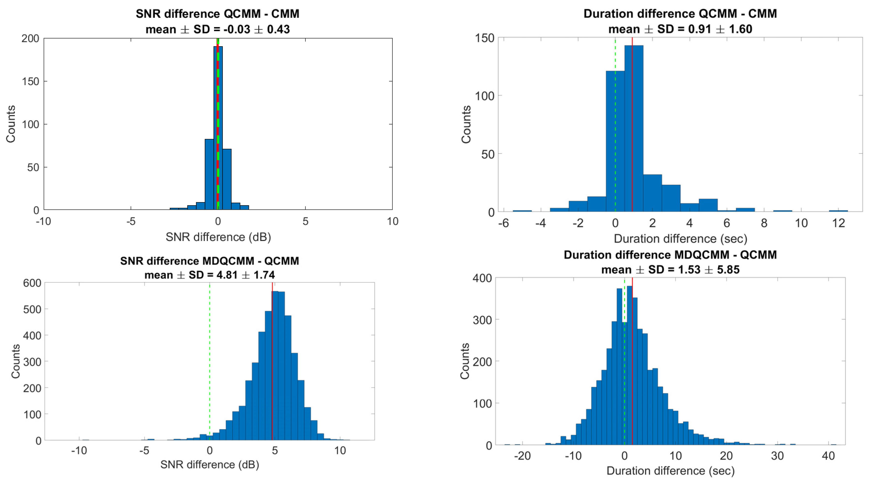
3.3. Quick Catalogue Maintenance Mode (QCMM) Processing

Keystone processing (KP) provides the ability to compensate for target range migration [24] and is typically applied prior to or in combination with pulse compression. For known satellites, TLE (or SP) propagations can be used to perform the KP. However, KP is not applicable to the BPST radar as the radar outputs range–time data x ( r ,   t ) and does not allow access to the pre-matched filtered data. However, a “Keystone-like” processing (KLP) approach can be applied in two steps using the TLE (or SP) propagation range R t , as illustrated in Figure 2:
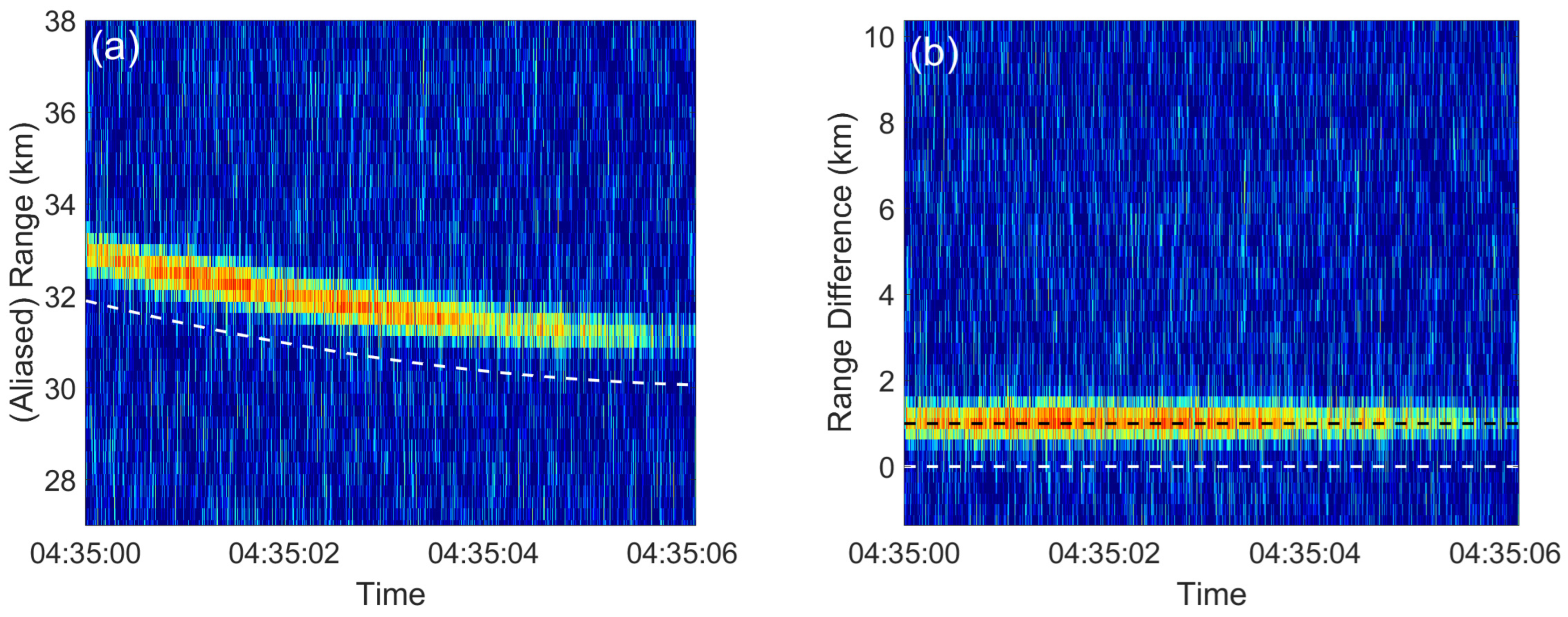
  • Range migration correction: Use the propagated range to convert the range–time data x ( r ,   t ) to “range difference” ( r ′) time data, x r r ,   t . This is achieved by interpolating x ( r ,   t ) across the range dimension or through a circular shift of the range–time data through the range dimension by ( R ( t ) / r ) samples, where represents the rounding-up operator and ∆r is the range resolution. The former option is applied in this paper, with the interpolation achieved using a simple Fourier method.
    x r ( r ,   t ) = F ( F 1 ( x r ,   t e x p 2 π i R t R a ) )
    where F represents the fast Fourier transform and R a is the range ambiguity.
  • Phase correction: The change in phase resulting from the change in the propagated range is corrected using the following:
x k ( r ,   t ) = x r ( r ,   t ) e x p 4 π i R ( t ) λ
The positive range difference illustrated in Figure 2 is typical of BPST observations and is due to signal propagation through the ionosphere (group retardation). This is discussed further in Section 3.5.
Having applied the KLP, the range difference time data can then be divided into overlapping CPIs and Doppler processed using an appropriate window to yield “range-difference Doppler-difference” data, x k ( r ,   d ) , which are then peak-processed in the manner described in [13]. Contiguous peaks with similar range and Doppler differences close to zero are then associated. If sufficient peaks are detected, an RSO detection is declared. The pseudo-code for QCMM processing is shown in Table 4.
The KLP obviates the need for acceleration processing and is consequently computationally less intensive than either DM or CMM. Like CMM, QCMM only allows the identification of catalogued objects and may miss objects with inaccurate propagation state vectors. As the KLP compensates for range migration, it allows the application of spectrograms to provide RSO micro-Doppler characterisation, as described in Section 6. As discussed in Section 2, the high orbital velocities of LEO RSOs motivate the use of overlapping CPIs for DM and CMM to mitigate range migration. Since the KLP removes range migration effects, QCMM can be applied using longer CPIs than DM and CMM, thereby increasing the coherent gain of the detections compared to DM and CMM and, consequently, the number of RSO detections.
An example of QCMM processing results for SL-8 R-B (NORAD ID 15032) on 22 March 2019 is shown in the top plots of Figure 3. These plots reveal a positive range difference (as also illustrated in Figure 1) and a negative radial velocity slope due to ionosphere signal propagation. These effects are discussed further in Section 3.5.

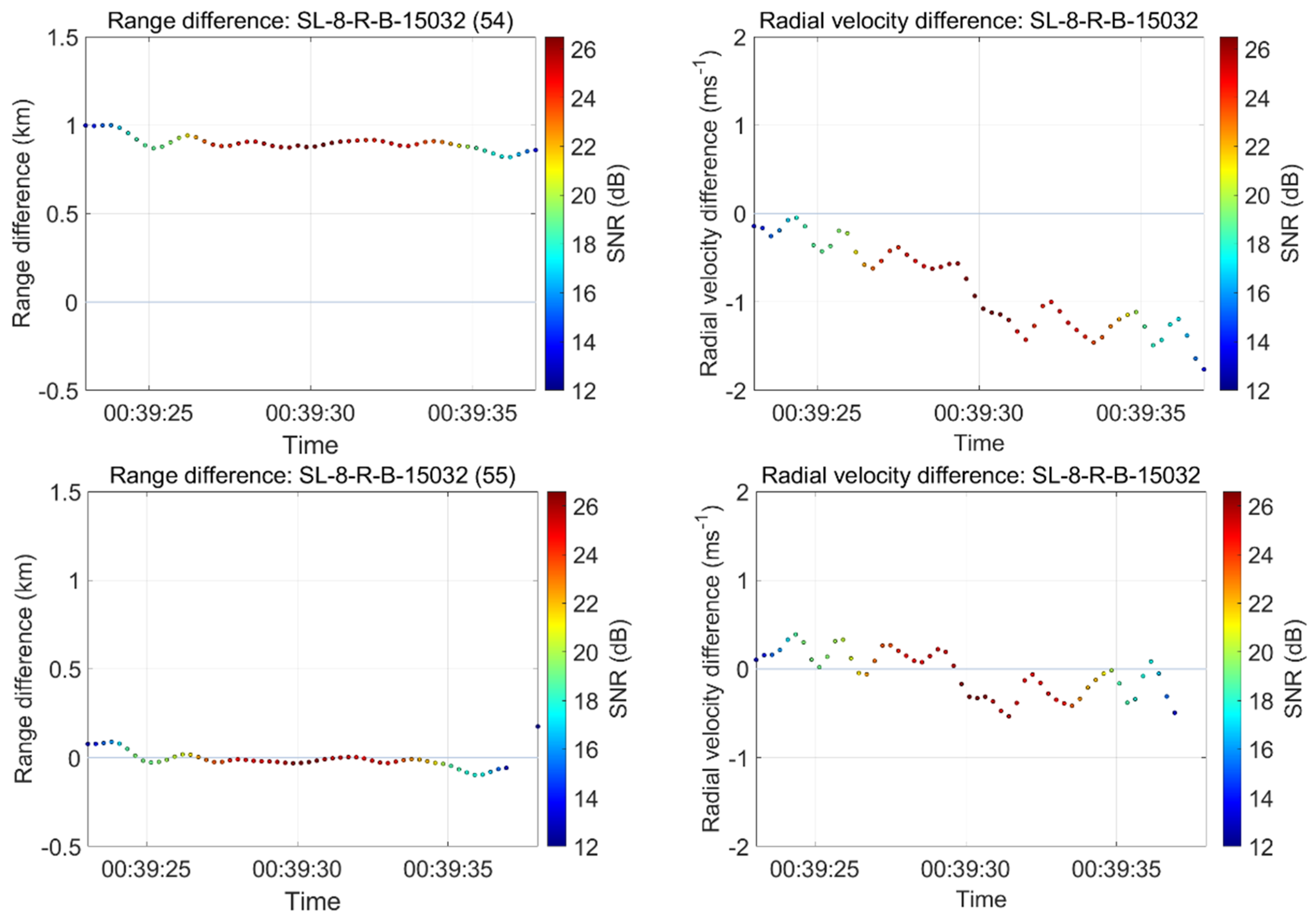
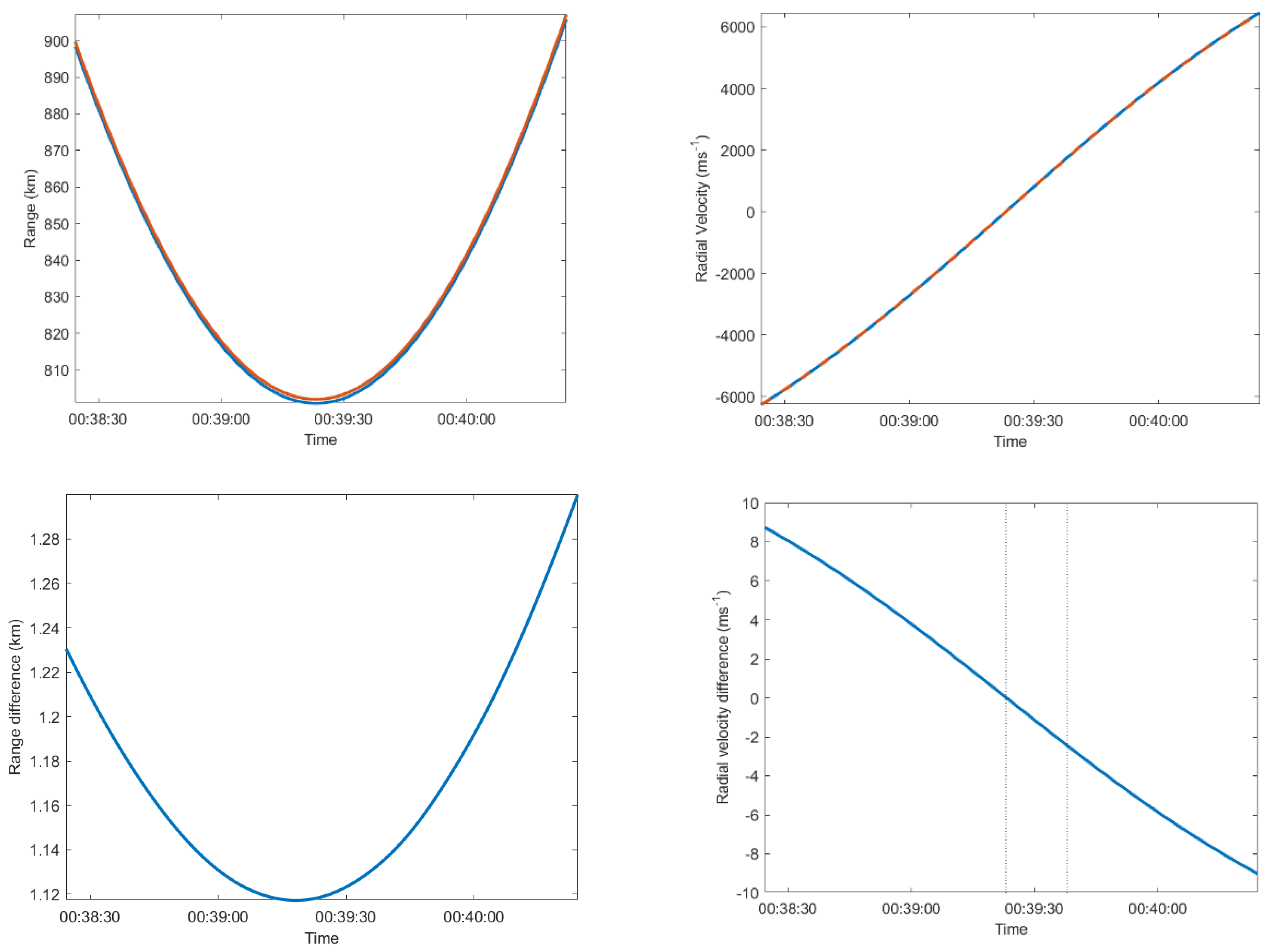
3.4. Matched Duration Quick Catalogue Maintenance Mode (MDQCMM) Processing

As previously discussed, KLP allows the CPI length to be increased without coherent loss due to range migration. This has allowed the development of a further signal processing strategy, matched duration quick catalogue maintenance mode (MDQCMM), that abandons the use of overlapping CPIs. MDQCMM is applied using an array of start and end times, which define candidate CPIs. Peak detection is applied for each candidate, with the CPI yielding the maximum SNR defining the transit duration. MDQCMM consequently yields significant SNR gains compared to QCMM and is therefore expected to enhance the detectability of low SNR RSOs and, hence, increase the detection rate. Furthermore, as MDQCMM may result in longer CPIs than the fixed-length CPIs used for DM, CMM, and QCMM, it will also reduce the radial velocity uncertainty. Like CMM and QCMM, MDQCMM only allows the identification of known objects and may not detect RSOs with erroneous TLE state vectors. Pseudo-code for MDQCMM processing is shown in Table 5.
Figure 4 provides two MDQCMM processing examples. For THEOS (NORAD ID 33396), the SNR versus start/end time plot shows a single broad peak, and the range–Doppler plot shows a single distinct peak. However, for CZ 2C R-B (NORAD ID 43031), the SNR versus start/end time plot shows two distinct maxima, and the range–Doppler plot shows a “defocussed” single distinct peak. This occurs because there is a Faraday fade during the transit, and the coherent gain is reduced when the fade is included in the CPI. For reference, the SNRs and detection durations obtained for THEOS and CZ 2C R-B using QCMM and MDQCMM processing are shown in Table 6. While MDQCMM generates a single peak, the QCMM processing generates peaks every ≈0.25 s, and the median QCMM SNR is therefore used for this comparison. This comparison reveals that MDQCMM processing yields a larger SNR for both RSOs and a larger detection duration for THEOS. However, MDQCMM processing yields a smaller detection duration for CZ 2C R-B due to the aforementioned Faraday fade. These results emphasise that Faraday rotation can significantly compromise optimal BPST radar RSO detection.
For reference, the computation times of the signal processing modes described in this paper for a typical 1 min dwell using MATLAB 2023b on a Dell Precision 7560 laptop (Adelaide, Australia) are shown in Table 7.

3.5. Ionospheric Correction

Radars operating in the medium frequency to lower VHF bands suffer from group retardation and phase advance due to signal propagation through the ionosphere [20], where the measured range and phase exceed the actual values. The group R g and phase R p path ranges can be expressed as (from [21])
R g = c 2 0 R d r U ( r ) ,
R p = c 2 0 R d r v ( r ) ,
where c is the speed of light (ms−1), U ( r ) is the group velocity (ms−1), and v ( r ) is the phase velocity (ms−1). In the absence of a magnetic field, the group and phase velocity can be expressed in terms of the radar operation frequency f (Hz) and the plasma frequency f p ( r ) (Hz) (from [21]):
U r = c 1 f p 2 r f 2 ,
v r = c 1 f p 2 r f 2 .
The plasma frequency is given by (from [20])
f p r = N ( r ) e 2 4 π m ϵ 0 ,
where N r is the electron density (m−3), e is the electron charge (Coulombs), m is the electron mass (g), and ϵ 0 is the permittivity of free space (m−3g−1s4A2).
Figure 5 illustrates the impact of ionospheric propagation using the SP propagations for SL-8 R-B (NORAD ID 15032) on 22 March 2019. These results were generated using the electron density profile obtained using the International Reference Ionosphere (IRI) 2016 model [25]. The top plots show the actual range and radial velocity and those obtained incorporating ionospheric propagation, hereafter the “effective” range and radial velocity. Although the effective range clearly exceeds the actual range (i.e., group retardation), the effective radial velocity appears to overlay the actual radial velocity. The bottom plots illustrate the range and radial velocity differences (effective minus actual). The range difference varies between 1.12 and 1.3 km, with the minimum range difference obtained when the RSO passes through the point of closest approach, where the ionospheric path length is minimised. Although the effective radial velocity appears to overlay the actual radial velocity, there is actually a small radial velocity difference that varies between ± 8 ms−1, which is a small fraction (0.013) of the radial velocity variation. The radial velocity difference passes through zero as the RSO passes through the point of closest approach. The radial velocity difference exhibits a negative slope and shows excellent agreement with the radial velocity difference observed in the top right plot of Figure 3, indicating that the negative phase slope observed in that plot is the result of ionospheric propagation.
Compensation for the effects of group retardation and phase advance can be performed by replacing the propagation range R ( t ) by R g ( t ) in (1) and by R p ( t ) in (2). The QCMM processing results for SL-8 R-B incorporating this correction using the International Reference Ionosphere (IRI) 2016 model are shown in the bottom plots of Figure 3. These plots reveal that the positive range difference and negative radial velocity slope observed without ionospheric correction have been rectified. Ionospheric correction also results in benefits for MDQCMM processing as the phase advance correction reduces the Doppler spread of the peak, thereby increasing the SNR and improving peak detectability.

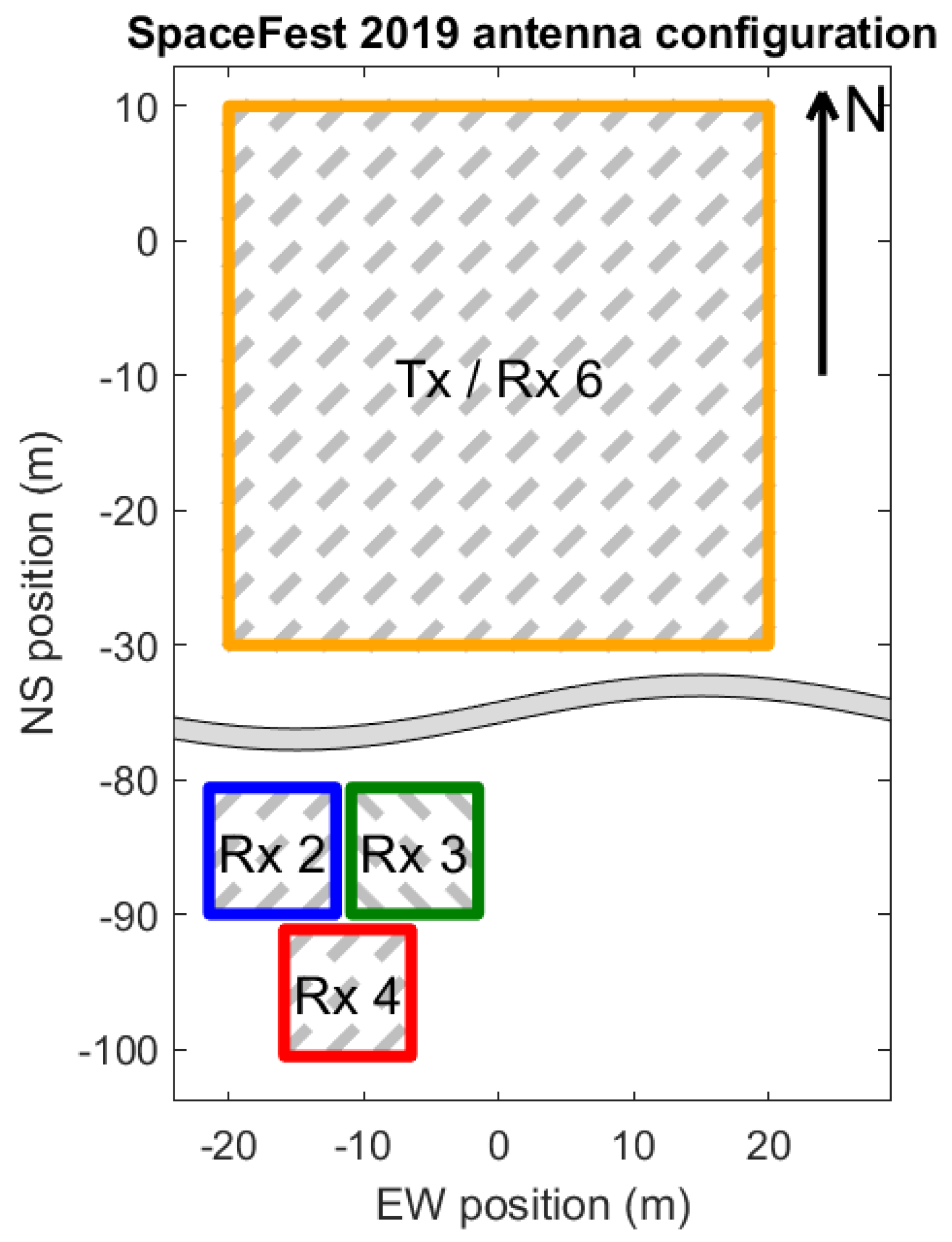
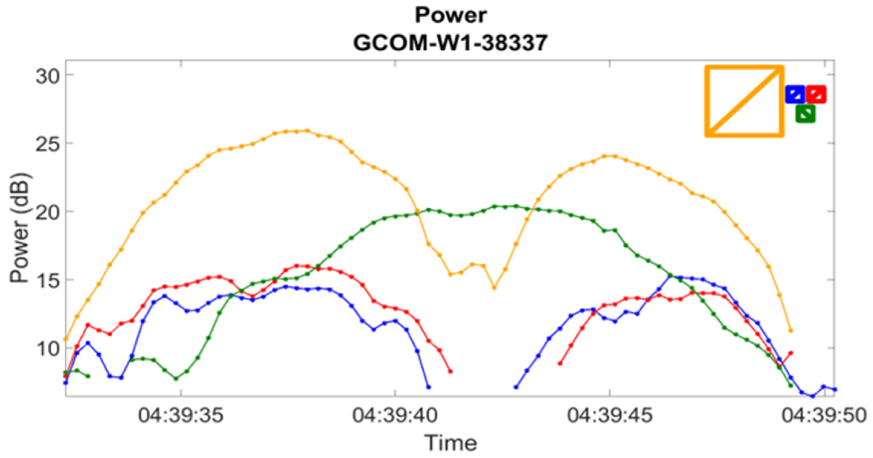
3.6. Use of Auxiliary Antennae Arrays

As described in Section 2, the BPST main array uses only one of the six available receivers. It was, therefore, decided to reconfigure the radar to connect three of the additional receivers typically used for meteor observations to three sets of co-located 3 × 3 Yagi arrays installed for boundary layer radar (BLR) observations [15]. Unless otherwise indicated, all results presented in this paper use the main array only.
In order to investigate the aforementioned Faraday rotation effects in more detail, the polarisation of one group of nine antennae was rotated to be perpendicular to that of the main array and the other two groups of antennae. Figure 6 shows typical RSO observations obtained using the four antenna arrays. Where the three identically polarised arrays (indicated by yellow, blue, and red lines) show a null at around 4:39:42, the perpendicularly polarised antenna shows a peak. This is the behaviour expected for Faraday rotation, whereby the received signal amplitude maximises (minimises) when the plane of polarisation of the incident signal is identical (perpendicular) to the antenna polarisation [21]. The fact that the observations shown in Figure 6 are typical confirms that the rapid amplitude fading reported in [13] is most likely attributable to Faraday rotation.

4. Standard Mode Results

4.1. Special Perturbation (SP) Data Comparisons

The BPST radar was operated using standard mode parameters for ten days, including the five days of SpaceFest 2019, 22 to 26 March, 27 to 29 March, and 1 and 2 April. All processing was applied using a CIT length of 2048 samples (≈2 s) with a 256 sample stepsize (≈0.25 s), resulting in an oversampling factor of eight. MDQCMM was applied using CIT start/end time increments of 1024 samples (≈1 s). A peak SNR threshold of 12 dB was applied. A minimum detection duration threshold of 5 s was required to constitute RSO detection, allowing discrimination of RSOs from long-lived meteor echoes, such as overdense or nonspecular echoes [13]. Unless otherwise indicated, the results presented in this section incorporate ionospheric correction, as described in Section 3.5.
The detection statistics for the ten days of standard mode observations are shown in Table 8. The results indicate average DM, QCMM, and MDQCMM daily count rates of 360, 450, and 590, respectively. The MDQCMM count rates represent a three-fold increase compared to the count rates reported in [13], indicating the success of the revised observation strategy and the signal processing improvements. The application of ionospheric correction increases the average QCMM and MDQCMM count rates by approximately 8 and 15 RSOs per day. A total of 2202 unique RSOs were detected using MDQCMM. Note that the variation in the daily detection rates is loosely correlated with the age of the TLEs used to produce the beam schedule.
In order to understand the relative daily count rates obtained using the DM, QCMM, and MDQCMM processing, Figure 7 shows histograms of the SNR and detection duration differences for common RSOs detected using QCMM and CMM and MDQCMM and QCMM. While MDQCMM generates a single peak, the CMM and QCMM processing generates peaks every ≈0.25 s. The median SNR is therefore used for the CMM and QCMM comparisons. For the QCMM and CMM comparison, the SNRs are roughly comparable, but QCMM yields a mean duration increase of 0.91 s. This results in a greater number of RSOs exceeding the 5 s detection threshold. For the MDQCMM and QCMM comparison, MDQCMM yields a mean SNR improvement of 4.81 dB, and the mean duration increase is 1.53 s. Note that the detection duration difference histogram exhibits a significant number of peaks with duration differences less than zero. This is due to the impact of Faraday fading on the MDQCMM processing, as discussed in Section 3.4.
The height, detection duration and RCS distribution of the MDQCMM results are shown in Figure 8. The lowest detection height was 341.2 km (SZ 11 MODULE, NORAD ID 41868). A total of 23 medium Earth objects (MEOs, 2000 km to 35,786 km) were detected, with a largest detection height of 2975.4 km (MIDAS 5 STRONGBACK 271), respectively. The histogram shows distinct peaks at 800, 1000, and 1200 and a broader peak at 1450 km. The 800 km peak is predominantly due to satellites with heights of 792 ± 2 km, comprising mainly Iridium (e.g., IRIDIUM-117, NORAD ID 42808) and Orbcomm-FM (e.g., OBRCOMM-FM-16, 25417) satellites. It is worth noting that the use of multiple PRFs avoids histogram “gaps” observed in [13], where pulse blanking resulted in gaps spaced at multiples of the range ambiguity. Detection durations between the minimum detection threshold of 5 s up to 50 s are observed. The larger durations are observed for objects with larger heights. As the beam area increases with height, higher objects consequently take longer to transit the BPST beams. The RCS values have been calculated using the technique described in [13], as described in Section 3.2. Figure 8 indicates that the MDQCMM processing is able to detect RSOs with RCS values as low as −14 dBm2 (i.e., 0.04 m2). Note that a common first-order detection sensitivity figure of merit of a radar is the minimum detectable RCS at a 1000 km range from both the radar transmitter and receiver. The minimum detectable RCS at 1000 km obtained using MDCMM processing is −10.97 dBm2 (0.09 m2).
As discussed in Section 2, the BPST radar main array uses a single receiver and is unable to measure the angular position of the detected RSOs. However, the propagation state vectors can be used to infer the angular position, assuming the state vectors are accurate, which is generally the case for the SP perturbations. Figure 9 shows the angular positions expressed in terms of cartesian zenith angles and latitude/longitude obtained using QCMM for the ten days of observations. The cartesian zenith angles are colour coded by “uncalibrated power”, which is the measured power (in squared A/D units) corrected for RCS and the fourth power of the RSO range in accordance with the radar equation. The uncalibrated power attempts to remove range and RCS effects from the power measurements, leaving only the effects associated with the radar antenna pattern. The colour coding clearly traces out the antenna pattern of the five BPST radar beams, confirming that the beam steering is functioning as intended.
In order to re-emphasise the advantages of using SP data in comparison to TLE/SGP4 data as highlighted in [13], Figure 10 shows a comparison of the radial velocity differences using SP perturbations and to TLE/SGP4 obtained using QCMM processing. The mean and standard deviation obtained using the SP estimates are substantially smaller than the TLE/SGP4 estimates. The SP estimates indicate that the errors in the BPST radial velocity estimates are of the order of 1 ms1. The accuracy of the BPST radial velocity estimates is investigated further in the following section.

4.2. International Laser Ranging Service Data Comparisons

The International Laser Ranging Service (ILRS) was established in September 1998 to support programs in geodetic, geophysical, and lunar research activities and to provide the International Earth Rotation Service with products important to the maintenance of an accurate International Terrestrial Reference Frame [26]. The ILRS currently includes more than 40 satellite laser ranging stations and routinely tracks about 20 retroreflector-equipped satellites, which are used to provide precise ephemerides that are made available at https://ilrs.gsfc.nasa.gov (accessed on 26 March 2024).
Table 9 shows a comparison of the radial velocity differences obtained using TLE/SGP4 data, SP data, and ILRS ephemerides, the latter both without and with ionospheric correction, as described in Section 3.5. Although the mean (i.e., bias) of ILRS radial velocity differences are larger than the SP estimates, the standard deviation obtained using the ILRS ephemerides is substantially smaller than both the SP and TLE/SGP4 estimates. These results suggest that the radial velocity accuracy of the BPST radar is better than 1 ms−1.
TerraSAR-X (NORAD ID 33605) and TanDEM-X (NORAD ID 31698) are a pair of retroreflector-equipped satellites that contribute to the ILRS data-set. The satellites fly in a closely controlled formation with a typical separation of between 250 and 500 m. Figure 11 illustrates the range and radial velocity difference peaks obtained for QCMM processing using the TanDEM-X ILRS ephemerides on 1 April 2019 and clearly shows two sets of peaks. Given the use of TanDEM-X ephemerides and assuming the ionospheric correction is correct, the range and radial velocity difference peaks for TanDEM-X should be close to zero, as indicated by the solid grey line. The range and radial velocity difference peaks should correspond to the difference between the TanDEM-X and TerraSAR-X ephemerides, as indicated by the dashed line. Thus, despite the small separation between the two satellites, both satellites have been detected and are easily distinguishable, with Figure 11 indicating that the two sets of peaks correspond to TanDEM-X (matching the solid line) and TerraSAR-X (matching the dashed line).

5. High-Range Resolution Mode Results

In [13], it was suggested that the BPST radar may be able to accurately measure total electron content (TEC) using measurements of the group retardation of LEO RSOs, i.e., the range difference between the estimated and predicted RSO ranges. Further, it was also suggested that the diversity of RSO heights may allow the BPST radar to estimate electron density profiles of the top side of the ionospheric F2 layer.
TEC measurements are typically made using ground-based dual frequency reception of GNSS satellite signal transmissions [27]. The TEC is defined as the number of free electrons in a column of a unit cross-sectional area along the ray path from the transmitter to the receiver end. The TEC measurement that characterises the ionosphere and plasmasphere for a particular location is obtained when the satellite is exactly overhead or above the location and is known as the vertical TEC (VTEC). Slant TEC is defined as the electron column density along an (oblique) line of sight. In the conversion of slant TEC to vertical TEC, it is often assumed that the ionosphere and plasmasphere are horizontally stratified and spatially uniform. Further, the ionosphere is typically simplified to be a thin layer at a fixed altitude of 350–400 km above the Earth’s surface [28]. GNSS TEC measurements are also subject to biases due to differential code biases and cycle slips.
The measurement of the range difference of RSOs allows the TEC to be estimated using (from [21])
T E C   r f 2 40.3 × 10 16   ,
where r is the estimated range difference, f is the radar operating frequency, and TEC is measured in TEC units (TECUs). This equation assumes f f H , where f H is the gyro-frequency. This condition is easily satisfied for the BPST radar, which operates at f = 55 MHz at a location where f H 1.5 MHz. The RSO range difference measurement avoids the aforementioned assumptions and biases inherent in GNSS TEC measurements. However, accurate measurements are reliant on both accurate range difference measurements and precise propagation state vectors.
A high-range resolution experiment was performed on 30 and 31 March 2019 using the high-resolution mode parameters shown in Table 3 to investigate the ability of the BPST radar to accurately measure TEC using measurements of the group retardation of LEO RSOs. A pulse width of 100 m was used to improve the range estimation accuracy compared to the standard mode experiment. The high-resolution mode parameters reduced the effective SNR of the radar measurements by approximately 3.5 dB compared to the standard mode experiment and consequently reduced the daily detection rates. In order to further improve the accurate group retardation measurements, Special Perturbations (SPs) propagations were used to provide accurate estimates of the RSO positions.
The MDQCMM peak range difference measurements obtained without ionospheric correction for 31 March 2019 are shown in Figure 12. Although the number of RSO observations is sparse, it is clear that the range difference (or group retardation) measurements follow the expected behaviour. The group retardation is larger during the day when solar radiation is available to produce ionisation. The maximum group retardation at around 0600 (1530 LT) is in agreement with IRI predictions. The group retardation increases monotonically with height, as most clearly observed around 0 UT, where it increases from 0.6 at 500 km to 0.85 at 1100 km. Finally, we note the presence of a pre-dawn group retardation minimum, as expected due to the pre-dawn foF2 minimum typically observed in the Australian region [29].

6. Spectrogram Analysis

In the situation where the TLE/SGP4 or SP propagations are sufficiently accurate, the application of QCMM and MDQCMM results in the RSOs being confined to a single range difference cell. In this case, a short-time Fourier transform (STFT) or spectrogram can be applied to observe the evolution of the Doppler characteristics of the RSO. In most cases, the spectrogram exhibits a single peak close to zero Doppler, as indicated for COSMOS-1844-1793 (NORAD ID 17973) in Figure 13. However, in some circumstances, the peak is displaced from 0 Hz. Such displacements are attributed to inaccuracies in the TLE/SG4 or SP propagations used in the analysis. In some circumstances, the spectrogram exhibits either periodic or random variation. As discussed in the following, we interpret the periodic variation as being due to RSO rotation and the random variation as being due to ionospheric effects.
The periodic variations observed in spectrograms obtained using the BPST radar have previously been used to investigate the micro-Doppler signatures of three non-operational satellites: RHESSI (NORAD ID 27370), TOPEX/Poseidon (NORAD ID 22076), and Telkom 3 (NORAD ID:38744) [30,31]. These papers also use computational electromagnetic modelling of simple computer-aided design (CAD) models to provide information on the satellite orientation and spin axis. Further, ref. [30] illustrates that the micro-Doppler periodicity of Telkom 3 decreased from 12 to 6.5 s between 2017 and 2020, indicating an increase in rotation rate over time.
Figure 13 illustrates two further examples of BPST radar spectrograms exhibiting micro-Doppler periodicity consistent with RSO rotation. The spectrogram for DMSP 5D 2 F8 USA (NORAD ID 18123) exhibits a periodicity of approximately 6 s, best illustrated in the segment between 21:10:20 and 21:10:29. The spectrogram for NOAA-16 (26536) exhibits a periodicity of approximately 4 s. In this example, Faraday fading around 12:29:23 appears to slightly disrupt the periodicity. The spectrogram for DELTA 1 DEB (8964) does not exhibit micro-Doppler periodicity; rather, it indicates symmetric sidebands spaced at approximately 1.6 Hz intervals. This is consistent with a 1.6 Hz amplitude modulation of the radar cross-section (RCS), suggesting that the RSO is rotating. Although this spectrogram cannot be used to distinguish micro-Doppler features, it provides information on the rotation rate of the RSO. Determination of the actual rotation rate requires additional information on the shape of the RSO. For instance, if the RSO has a cylindrical shape, the 1.6 Hz amplitude modulation would correspond to a rotation rate of 0.8 Hz.
Figure 14 illustrates two examples of BPST radar spectrograms exhibiting random variations obtained from observations of two Starlink satellites. Since numerous transits of the same satellites have been observed without such random variations, we attribute the variations to ionospheric phenomena occurring during the observations. The random variations obtained using the BPST and DSTG HF LOS radars have been investigated [32,33] and attributed to two sources. The first source is ionospheric plasma instabilities in the 0–0.46 Hz frequency range. The second source was identified as Electromagnetic Ion Cyclotron (EMIC) plasma waves in the 0.1–0.5 Hz frequency range, propagating parallel to the Earth’s surface in a waveguide centred at an altitude of 250 km. EMIC waves can last several hours, while plasma irregularities last only 10 s [33]. These phenomena produce electron density perturbations along the signal path between the radars and the RSO, which manifest as variations in the measured Doppler. These variations result in a small increase in the uncertainty of the Doppler measurements [32].

7. Discussion

This current paper introduces new experimental parameters, beam scheduling, and signal processing capabilities that increased the daily count rates observed by the radar from between 150 and 200 RSOs to between 480 and 630 RSOs, representing a three-fold increase. As the introduction of the new experimental parameters and beam scheduling were made simultaneously, it is difficult to isolate the contribution of these two new components. However, Table 8 illustrates the contribution of the signal processing advances, illustrating that QCMM and MDQCMM analyses increase the count rates by approximately 1.3 and 1.6 compared to DM. The results indicate that a minimum detectable RCS at 1000 km of −10.97 dBm2 (0.09 m2) was observed. The results also indicate that the radial velocity error measured by the BPST radar is less than 1 ms−1. This is a remarkable result, given that the orbital velocity of a typical LEO object is around 8 kms−1. The results further indicate that the TanDEM-X and TerraSAR-X satellites, which are typically separated by between 250 and 500 m, were both detectable and distinguishable. Despite the increased count rates provided by the new QCMM and MDQCMM analyses, they are unable to detect uncatalogued RSOs or RSOs with inaccurate propagation state vectors. This suggests that there is a role for both DM (detection of uncatalogued RSOs) and MDQCMM (catalogue maintenance) for future BPST RSO observations.
This paper also demonstrates a method to compensate for ionospheric group retardation and phase advance. The success of this compensation is dependent on the accuracy of the electron density profile used to perform the compensation. Ideally, the electron density profile could be provided by a co-located vertical incidence ionospheric sounder (VIS) [34] or a real-time ionospheric model (RTIM) [35,36]. However, for locations such as Buckland Park, where neither a VIS or RTIM is available, a climatological model such as the International Reference Ionosphere (IRI) must be used. However, we note that comparisons between the IRI and ionospheric sounder electron densities have highlighted limitations with the IRI model [37].
An auxiliary antenna array, including three sets of nine antennae, including one set of antennae with dipoles aligned perpendicularly to the main array, was used to confirm that signal fading observed by the BPST radar is most likely the result of Faraday rotation effects. We note that Faraday rotation could potentially be eliminated through the transmission of circularly polarised signals, representing a potential avenue for further research.
The earlier study [13] suggests that BPST RSO ionospheric group retardation measurements may provide a means to perform total electron content (TEC) measurements. However, the results indicated that a further increase in range resolution would be required to accurately measure TEC. Observations using a significantly increased range resolution were performed prior to the conclusion of SpaceFest 2019. However, the increased range resolution was achieved at the expense of a sensitivity reduction of 3.5 dB. Although the number of RSO observations was sparse, the group retardation measurements clearly followed the expected diurnal behaviour. The results also suggest that electron density profile determination will require either a significantly higher number of RSOs than were in orbit at the time of these measurements or the use of a significantly higher-power aperture product than that currently used by the BPST radar. Regarding the former, we note that there are currently a significantly larger number of RSOs in LEO orbits than at the time of these measurements, including approximately 5500 Starlink satellites. However, as will be discussed in a future paper, the frequent manoeuvres made by Starlink satellites to maintain constellation result in the propagation estimates becoming “stale”, such that they do not accurately predict the state vectors at the observation time. Regarding the use of a significantly higher transmit power by the BPST radar, we note that there are a number of mesospheric–stratospheric–tropospheric (MST) radars operating at similar frequencies to the BPST radar that use significantly higher transmit power. The middle and upper atmosphere (MU) radar is located at the Shigaraki Observatory, Kyoto University, Japan [38], and operates at 46.5 MHz, with a peak power of 1 MW (25 times that of the BPST radar) and a beam width of 3.6°. The MAARSY mesosphere–stratosphere–troposphere (MST) is located in Andenes, Norway [39], and operates at 53.5 MHz, with a peak power of 800 kW (20 times that of the BPST radar) and a beam width of 3.6°. The MU and MAARSY radars may provide sufficient power aperture product to allow the detection of sufficient RSOs to allow the estimation of electron density profiles. We also note that the analysis described in this paper has been successfully applied to a small subset of data from the MAARSY radar.
The application of QCMM and MDQCMM results in the RSOs being confined to a single range difference cell. This allows a short-time Fourier transform (STFT), or spectrogram, to be applied to observe the evolution of the Doppler characteristics of the RSO. In some circumstances, the spectrogram exhibits either periodic variations attributed to RSO rotation or random variation due to ionospheric plasma instabilities and Electromagnetic Ion Cyclotron (EMIC) plasma waves [32,33]. The periodic variations provide micro-Doppler information that can be combined with simulated signatures from computational electromagnetic modelling of simple computer-aided design (CAD) models to provide further interpretation of the RSOs, such as orientation and spin axis. We believe the EMIC wave observations represent the first time that radar has been used to observe such waves, and we also believe that, during summer, radar may provide a more sensitive measure of the plasma waves than ground and space-borne magnetometers normally used to detect these waves.
The QCMM analysis is computationally non-intensive and can be applied in real time using a PC with modest computational capabilities. This has been exploited by introducing a second dedicated RSO analysis PC to the BPST radar to perform real-time QCMM analysis. This has allowed the QCMM analysis to be applied to data collected for the Doppler beam steering (DBS) analysis of tropospheric and stratospheric winds for which the radar was originally designed [15]. Despite the data acquisition parameters being non-optimal for RSO observations, daily count rates of up to 100 RSOs have been obtained. These count rates could potentially be increased by using the beam scheduling strategy described in this paper, subject to meeting the operational requirements of the DBS analysis, which requires each of the five available beam directions to be used once every five minutes. Noting that the Bureau of Meteorology (BoM) operates four ST radars similar to the BPST throughout Australia, as well as nine smaller, lower-powered boundary layer radars, the BPST QCMM analysis could potentially be applied to data collected by the BoM network to improve Australia’s SDA measurement capabilities.
A limitation of the BPST radar configuration used in this paper is that the main array is connected to a single receiver, and the radar is consequently unable to estimate the RSO angle of arrival (AOA). For the subsequent SpaceFest 2020 campaign, the BPST radar main array was separated into a central 6 × 6 array connected to one receiver, surrounded by eight 3 × 3 arrays, each connected to a separate receiver, thereby providing an RSO AOA estimation capability. Further, a remote receiving array of three 3 × 3 antenna arrays was deployed 35 km south of the BPST radar to allow bistatic measurements. These results will be described in a subsequent paper.

8. Conclusions

This paper follows up on an initial investigation of the use of a VHF wind profiling radar for observing RSOs. The radar was operated during the Australian Defence “SpaceFest” 2019 activity, incorporating new beam scheduling and signal processing capabilities. The beam scheduling capability used two-line element propagations to determine the appropriate beam direction to use to observe the transiting RSOs. The signal processing capabilities used a Keystone transform-like approach to correct for range migration, allowing the coherent integration time to be increased to improve the SNR of the observed targets, thereby increasing the detection rate.
The results reveal that 5874 objects were detected over 10 days, with 2202 unique objects detected, representing a three-fold increase in the detection rate over previous observations. A minimum detectable RCS at 1000 km of −10.97 dB m2 (0.09 m2) was observed. The effects of Faraday rotation resulting from the use of linearly polarised antennae was demonstrated. The radar’s utility for providing total electron content (TEC) measurements was illustrated using a high-range resolution mode and high-precision ephemeris data. The short-term Fourier transform was applied to demonstrate the radar’s ability to determine RSO rotation characteristics and short-period ionospheric perturbations.

Author Contributions

Conceptualisation, D.A.H.; methodology, D.A.H., A.J.S. and C.L.A.; software, D.A.H., A.J.S. and C.L.A.; validation, D.A.H.; formal analysis, D.A.H.; investigation, D.A.H.; resources, I.M.R.; data curation, D.A.H. and A.J.S.; writing—original draft preparation, D.A.H.; writing—review and editing, D.A.H., A.J.S., C.L.A. and I.M.R.; visualisation, D.A.H.; supervision, D.A.H.; project administration, I.M.R.; funding acquisition, I.M.R. All authors have read and agreed to the published version of the manuscript.

Funding

Funding for the BP ST radar was provided by the University of Adelaide, ATRAD Pty Ltd., the Australian Research Council grants DP0878144 and DP1096901 and by the Adelaide University ARC Small Grants Scheme. A.J.S. was supported by an Australian Government Research Training Program scholarship.

Data Availability Statement

Data supporting reported results can be found at https://doi.org/10.25909/25044581 (accessed on 26 March 2024).

Acknowledgments

The authors thank Brendan Hennessy for his insightful comments. The involvement of I.M.R. and C.L.A. was supported by ATRAD Pty Ltd. Data. The TLE and SP data used in this paper were obtained from the SpaceTrack web site https://www.space-track.org (accessed on 26 March 2024) The ILRS data were obtained from https://ilrs.gsfc.nasa.gov (accessed on 26 March 2024).

Conflicts of Interest

Authors I.M.R. and C.L.A. are employed by ATRAD Pty. Ltd. The remaining authors declare that the research was conducted in the absence of any commercial or financial relationships that could be construed as a potential conflict of interest.

References

  1. Boley, A.C.; Byers, M. Satellite mega-constellations create risks in Low Earth Orbit, the atmosphere and on Earth. Sci. Rep. 2021, 11, 10642. [Google Scholar] [CrossRef] [PubMed]
  2. Mann, A. Starlink: SpaceX’s Satellite Internet Project. 2021. Available online: https://www.space.com/spacex-starlink-satellites.html (accessed on 26 March 2024).
  3. Patel, N.V. Averting space doom. IEEE Spectr. 2015, 52, 16–17. Available online: https://ieeexplore.ieee.org/abstract/document/7024495 (accessed on 26 March 2024).
  4. ESA. Spacecraft Dodges Large Constellation. Available online: https://www.esa.int/Safety_Security/ESA_spacecraft_dodges_large_constellation (accessed on 26 March 2024).
  5. Smith, C.H.; Greene, B.; Bold, M.; Drury, R. Development of a new SDA facility at Learmonth Australia. In Proceedings of the Advanced Maui Optical and Space Surveillance Technologies Conference, Maui, HI, USA, 11–14 September 2018. [Google Scholar]
  6. Space Surveillance Telescope Declared Operational—Australian Defence Magazine. Available online: https://www.australiandefence.com.au/news/space-surveillance-telescope-declared-operational (accessed on 26 March 2024).
  7. LeoLabs Commits to WA for Next Space Radar. October 2021. Available online: https://www.wa.gov.au/government/announcements/leolabs-commits-wa-next-space-radar (accessed on 26 March 2024).
  8. Cohen, G.; Afshar, S.; van Schaik, A.; Wabnitz, A.; Bessell, T.; Rutten, M.; Morreale, B. Event-based sensing for space situational awareness. In Proceedings of the Advanced Maui Optical and Space Surveillance Technologies Conference (AMOS), Maui, HI, USA, 19–22 September 2017. [Google Scholar]
  9. Frazer, G.J.; Meehan, D.H.; Warne, G.M. Decametric measurements of the ISS using an experimental HF line-of-sight radar. In Proceedings of the 2013 International Conference on Radar, Adelaide, SA, Australia, 9–12 September 2013. [Google Scholar]
  10. Frazer, G.J.; Rutten, M.; Cheung, B.; Cervera, M.A. Orbit determination using a decametric line-of-site radar. In Proceedings of the Advanced Maui Optical and Space Surveillance Technologies Conference (AMOS), Maui, HI, USA, 9–12 September 2014. [Google Scholar]
  11. Palmer, J.E.; Hennessy, B.; Rutten, M.; Merrett, D.; Tingay, S.; Kaplan, D.; Tremblay, S.; Ord, S.M.; Morgan, J.; Wayth, R.B. Surveillance of Space using passive radar and the Murchison Widefield Array. In Proceedings of the IEEE Radar Conference, Seattle, WA, USA, 8–12 May 2017; pp. 1715–1720. [Google Scholar]
  12. Hennessy, B.; Rutten, M.; Young, R.; Tingay, S.; Summers, A.; Gustainis, D.; Crosse, B.; Sokolowski, M. Establishing the Capabilities of the Murchison Widefield Array as a Passive Radar for the Surveillance of Space. Remote Sens. 2022, 14, 2571. [Google Scholar] [CrossRef]
  13. Holdsworth, D.A.; Spargo, A.J.; Reid, I.M.; Adami, C. Low Earth Orbit Object Observations Using the Buckland Park VHF Radar. Radio Sci. 2020, 55, 2019RS006873. [Google Scholar] [CrossRef]
  14. Hall, T.D.; Duff, G.F.; Maciel, L.J. The Space Mission at Kwajalein. Linc. Lab. J. 2012, 19, 48–63. [Google Scholar]
  15. Dolman, B.K.; Reid, I.M.; Tingwell, C. Stratospheric tropospheric wind profiling radars in the Australian network. Earth Planets Space 2018, 70, 170. [Google Scholar] [CrossRef]
  16. Morris, R.J.; Murphy, D.J.; Vincent, R.A.; Holdsworth, D.A.; Klekociuk, A.R.; Reid, I.M. Characteristics of the wind, temperature and PMSE field above Davis, Antarctica. J. Atmos. Sol.-Terr. Phys. 2006, 68, 418–435. [Google Scholar] [CrossRef]
  17. Morris, R.J.; Klekociuk, A.R.; Holdsworth, D.A. First observations of Southern Hemisphere polar mesosphere winter echoes including conjugate occurrences at∼69 S latitude. Geophys. Res. Lett. 2011. [Google Scholar] [CrossRef]
  18. Spargo, A.J.; Reid, I.M.; MacKinnon, A.D. Multistatic meteor radar observations of gravity-wave–tidal interaction over southern Australia. Atmos. Meas. Tech. 2019, 12, 4791–4812. [Google Scholar] [CrossRef]
  19. McGeogh, J.; Jensen, J. Acceleration and Velocity Processing of HF Radar Signals; Technical Report; Naval Research Laboratory: Washington, DC, USA, 1967. [Google Scholar]
  20. Bird, D. Sharing Space Situational Awareness Data. In Proceedings of the Advanced Maui Optical and Space Surveillance Technologies Conference, Maui, HI, USA, 14–17 September 2010. [Google Scholar]
  21. Davies, K. Ionospheric Radio; IET: London, UK, 1990. [Google Scholar]
  22. Holdsworth, D.A.; Reid, I.M. Preliminary Count Rate Maximisation of the Buckland Park Interferometric Meteor Radar. In Proceedings of the Workshop on the Applications of Radio Science, Hobart, TAS, Australia, 18–20 February 2004. [Google Scholar]
  23. McCant, M. Median RCS Values. 2017. Available online: https://www.prismnet.com/~mmccants/catalogs/index.html (accessed on 21 May 2021).
  24. Perry, R.P.; DiPietro, R.C.; Fante, R.L. Coherent integration with range migration using keystone formatting. In Proceedings of the 2007 IEEE Radar Conference, Waltham, MA, USA, 17–20 April 2007; IEEE: Piscataway, NJ, USA, 2007; pp. 863–868. [Google Scholar]
  25. Bilitza, D.; Altadill, D.; Truhlik, V.; Shubin, V.; Galkin, I.; Reinisch, B.; Huang, X. International Reference Ionosphere 2016: From ionospheric climate to real-time weather predictions. Space Weather. 2017, 15, 418–429. [Google Scholar] [CrossRef]
  26. Pearlman, M.R.; Degnan, J.J.; Bosworth, J.M. The international laser ranging service. Adv. Space Res. 2002, 30, 135–143. [Google Scholar] [CrossRef]
  27. Klobuchar, J.A. Ionospheric effects on GPS. In Chapter 12 of Global Positioning System: Theory and Applications; American Institute of Aeronautics and Astronautics: Reston, VA, USA, 1996; Volume 1, p. 30. [Google Scholar]
  28. Seemala, G.K. Estimation of ionospheric total electron content (TEC) from GNSS observations. In Atmospheric Remote Sensing; Elsevier: Amsterdam, The Netherlands, 2023; pp. 63–84. [Google Scholar]
  29. Wilkinson, P.J. Predictability of ionospheric variations for quiet and disturbed conditions. J. Atmos. Terr. Phys. 1995, 57, 1469–1481. [Google Scholar] [CrossRef]
  30. Heading, E.; Nguyen, S.T.; Holdsworth, D.; Field, D.; Reid, I. Analysis of RF Signatures for Space Domain Awareness using VHF radar. In Proceedings of the 2022 IEEE Radar Conference (RadarConf22), New York City, NY, USA, 21–25 March 2022; IEEE: Piscataway, NJ, USA, 2022; pp. 1–6. [Google Scholar]
  31. Heading, E.; Nguyen, S.T.; Holdsworth, D.; Field, D.; Reid, I. Micro-Doppler Signature Analysis for Space Domain Awareness using VHF radar. Remote Sens. 2024, in press. [Google Scholar]
  32. Jonker, J.R.; Cervera, M.A.; Holdsworth, D.A.; Harris, T.J.; MacKinnon, A.D.; Neudegg, D.; Reid, I.M. Impact of Ionospheric Doppler Perturbations on Space Domain Awareness Observations. In Proceedings of the International Conference on Radar, Sydney, NSW, Australia, 6–10 November 2023. [Google Scholar]
  33. Jonker, J.R.; Cervera, M.A.; Harris, T.J.; Holdsworth, D.A.; MacKinnon, A.D.; Neudegg, D.; Reid, I.M. Observational evidence of EMIC waves propagating in the mid-latitude ionospheric waveguide using ground-based HF and VHF radar. Adv. Space Res. 2024. [Google Scholar]
  34. Harris, T.J.; Quinn, A.D.; Pederick, L.H. The DST group ionospheric sounder replacement for JORN. Radio Sci. 2016, 51, 563–572. [Google Scholar] [CrossRef]
  35. Barnes, R.I.; Gardiner-Garden, R.S.; Harris, T.J. Real time ionospheric models for the Australian Defence Force. In Proceedings of the Workshop for Applications of Radio Science (WARS), Leura, NSW, Australia, 20–22 February 2002. [Google Scholar]
  36. Reinisch, B.; Galkin, I.; Huang, X.; Vesnin, A.; Bilitza, D. The Ionosphere Real-Time Assimilative Model, IRTAM-A Status Report. In Proceedings of the EGU General Assembly Conference Abstracts, Vienna, Austria, 27 April–2 May 2014; Volume 16. [Google Scholar]
  37. Edwards, D.J.; Chambers, T.E.; Cervera, M.A. CLIMF2: A Climatological Model of the Ionospheric F2 Layer. Part 2: Validation and Comparison with IRI. Adv. Space Res. 2023. [Google Scholar] [CrossRef]
  38. Sato, T.; Kimura, I.; Kayama, H.; Furusawa, A. MU radar measurements of orbital debris. J. Spacecr. Rocket. 1991, 28, 677–682. [Google Scholar] [CrossRef]
  39. Renkwitz, T.; Stober, G.; Latteck, R.; Singer, W.; Rapp, M. New experiments to validate the radiation pattern of the Middle Atmosphere Alomar Radar System (MAARSY). Adv. Radio Sci. 2013, 11, 283–289. [Google Scholar] [CrossRef]
Figure 1. BPST radar main and auxiliary antenna arrays used for SpaceFest 2019.
Remotesensing 16 01252 g001
Figure 2. Example of application of “Keystone-like” processing. (a) Range–time power | x ( r ,   t ) | 2 for a transit of the rocket body SJ 16 02 (NORAD ID 41634) at 0:35 on 24 March 2019. The dashed white line indicates the predicted range obtained using SP propagation data. (b) Range difference time power | x r ( r ,   t ) | 2 after application of the first step of Keystone-like processing. The dashed white line indicates zero range, while the dashed black line indicates the range difference of maximum power. (c) Phase of the range difference time data x r ( r ,   t ) at the range difference indicated by the dashed black line in (b). (d) Phase of phase-corrected range difference time data x k ( r ,   t ) obtained after applying the final step of Keystone-like processing.
Remotesensing 16 01252 g002aRemotesensing 16 01252 g002b
Figure 3. Example of peak range difference (left) and radial velocity difference (right) obtained using quick catalogue maintenance (QCMM) mode processing for SL-8 R-B (NORAD ID 15032) on 22 March 2019, both without (top) and with (bottom) ionospheric correction applied.
Remotesensing 16 01252 g003
Figure 4. Example of application of matched duration quick catalogue maintenance mode (MDQCMM) for the THEOS satellite (NORAD ID 33396) at 00:13 (top) and for CZ 2C R-B (NORAD ID 43031) at 4:40 (bottom), both on 1 April 2019. The left plots show the SNR variation obtained over a grid of start and end times, with the diamond indicating the start/end time producing maximum SNR. The right plots show the range–Doppler display for the start/end time producing maximum SNR, with the plus sign indicating the interpolated peak position in the range difference/Doppler difference dimensions.
Remotesensing 16 01252 g004
Figure 5. Illustration of the effects of ionospheric propagation on the SP propagation state vectors of SL-8 R-B (NORAD ID 15032) on 22 March 2019. (Top left) Actual (blue) and estimated (red) range resulting from ionospheric propagation. (Top right) Actual (blue) and estimated (dashed red) radial velocity resulting from ionospheric propagation. (Bottom left) range difference (estimate minus actual). (Bottom right) radial velocity difference (estimate minus actual). The dashed lines indicate the start and end times of the detections shown in Figure 4.
Remotesensing 16 01252 g005
Figure 6. Illustration of the effects of Faraday rotation on the peak power estimates received on the BPST main array (yellow) and the three BLR arrays (blue, red, and green) for the GCOM-W1 satellite (NORAD ID 38337). The three identically polarised arrays (yellow, blue, and red) show a 10 dB null at around 4:39:42, while the array with perpendicular polarisation shows a peak.
Remotesensing 16 01252 g006
Figure 7. Detection duration (left) and RCS (right) histograms obtained using quick catalogue maintenance mode (QCMM, blue) and matched duration quick catalogue maintenance mode (MDQCMM) processing for standard mode observations. The red lines indicate the mean of the difference distribution, and the green dashed line indicates zero difference.
Remotesensing 16 01252 g007
Figure 8. Histogram of RSO heights (top left), duration (top right), and radar cross-section (bottom) obtained using matched duration quick catalogue maintenance mode (MDQCMM) processing for standard mode observations.
Remotesensing 16 01252 g008
Figure 9. Illustration of angular parameters of RSOs detected by the BPST radar from 22 to 29 March and 1 and 2 April using quick catalogue maintenance mode (QCMM). (Top) Cartesian zenith angle components colour coded by “uncalibrated power” (measured power corrected for the satellite range and RCS). The thick black circles indicates the theoretical half-power beam width of the radar, and the dashed circles indicate multiples or two, three and four times the beam width. (Bottom) Latitude and longitude colour coded by NORAD ID.
Remotesensing 16 01252 g009
Figure 10. Histograms of QCMM radial velocity differences obtained using TLE/SGP4 (left) and SP propagations (right) for the ten days of standard mode measurements. The means and standard deviations of the distributions are indicated in the plot titles.
Remotesensing 16 01252 g010
Figure 11. Range (left) and radial velocity difference (right) peaks obtained using quick catalogue maintenance mode (QCMM) processing using the ILRS ephemerides for TanDEM-X (NORAD ID 33605) on 1 April 2019. The solid grey lines show zero range and radial velocity difference for TanDEM-X, while the grey dashed lines show the corresponding zero range and Doppler differences for TerraSAR-X (NORAD ID 31698).
Remotesensing 16 01252 g011
Figure 12. Range difference (i.e., ionospheric group retardation) as a function of height and time obtained using matched duration quick catalogue maintenance mode (MDQCMM) processing on 31 March 2019.
Remotesensing 16 01252 g012
Figure 13. Example of spectrograms indicating non-rotating and rotating RSOs. (Top left) COSMOS-1844-1793 (NORAD ID 17973). (Top right) DMSP 5D 2 F8 USA (18123). (Bottom left) NOAA-16 (26536). (Bottom right) DELTA 1 DEB (8964). The top left plot represents an example of a non-rotating RSO, while the remaining plots indicate examples of rotating RSOs.
Remotesensing 16 01252 g013
Figure 14. Example of spectrograms for two Starlink satellites illustrating random Doppler variations. (Left) Starlink 5420 (NORAD ID 54798), (right) Starlink 6226 (56544).
Remotesensing 16 01252 g014
Table 1. BPST radar parameters (from [13]).
ParameterValue(s)
Frequency, f (MHz)55
Maximum Transmit Power (kW)40 (12 4 kW modules, i.e., 48 kW at the transmitter)
Maximum Duty Cycle (%)10
Pulse TypesMonopulse, Barker, and Complementary Codes
Receiver Filter Widths (kHz)4, 8, 16, 32
Pulse-to-pulse Frequency Extent±50 kHz
Maximum Pulse Repetition Frequency (kHz)20
Number of Transmit Antennae144
Number of Receive Antennae144 (Main array), 5 (Meteor array)
Combined Tx/Rx Main Array Beam Width (°)7
Pulse Widths (m)100–4000
Pulse Widths (μs)0.67–26.67
Number of Receivers6 (1–5: Meteor array, 6: Main array)
Range Sampling Resolution, Δr (km)0.05–2
Beam Directions (Azimuth, Zenith) (degrees)(0, 0) “Vertical”, (0, 15) “North”, (90, 15) “East”
(180, 15) “South”, (270, 15) “West”
Table 2. Pseudo-code for Detection Mode (DM) and Catalogue Maintenance Mode (CMM).
Detection Mode
Loop over overlap processing intervals
   Data selection
   Acceleration processing
   Doppler processing
   Peak detection and interpolation
   Whitening
   Peak selection
Loop over concurrent propagation state vectors
   Associate peaks to propagation state vectors
   Declare RSO detected if sufficient associated peaks
Catalogue Maintenance Mode
Loop over concurrent propagation state vectors
   Data selection
   Loop over overlap processing intervals
   Acceleration processing
   Doppler processing
   Peak detection and interpolation
   Whitening
   Peak selection
   Associate peaks to propagation state vectors
   Declare RSO detected if sufficient associated peaks
Table 3. BPST radar parameters.
ParameterStandard ModeHigh Resolution
Pulse repetition frequency (Hz)1953, 20009950, 10,000
Number of coherent averages26
Dwell length (s)5656
Range ambiguity (km)76.8, 7515.08, 15
Radial velocity resolution 1 (ms−1)1.361.36
Pulse type13-bit Barker13-bit Barker
Pulse width (km)0.50.1
Pulse width (μs)3.330.67
Receiver filter width (kHz)128640
Minimum range (km)7.52.5
Maximum range (km)6912.5
Range sampling resolution (km)0.250.1
1 2 s coherent processing interval.
Table 4. Pseudo-code for Quick Catalogue Maintenance Mode (QCMM).
Loop over Concurrent Propagation State Vectors
   Apply Keystone-Like Processing
   Loop over Overlap Processing Intervals
   Data selection
   Acceleration processing
   Doppler processing
   Peak detection and interpolation
   Whitening
   Peak selection
   Associate peaks to zero range and Doppler difference
   Declare RSO detected if sufficient associated peaks
Table 5. Pseudo-code for Matched Duration Quick Catalogue Maintenance Mode (MDQCMM).
Loop over Concurrent Propagation State Vectors
   Apply Keystone-Like Processing
   Loop over Overlap Processing Interval Start Times
   Loop over Overlap Processing Interval End Times
    Data selection
    Acceleration processing
    Doppler processing
    Peak detection and interpolation
    Whitening
    Peak selection
    Associate peaks to zero range and Doppler difference
    Declare RSO detected if sufficient associated peaks
   If RSO detected, select start and end times with yielding maximum SNR
Table 6. SNRs and detection durations obtained using QCMM and MDQCMM processing for the THEOS (NORAD ID 33396) and CZ 2C R-B (NORAD ID 43031).
RSOQCMM
SNR (dB)
MDQCMM SNR (dB)QCMM
Duration (s)
MDQCMM
Duration (s)
THEOS23.3229.9012.8416.77
CZ 2C R-B26.1930.9616.9010.24
Table 7. Computation times of different signal processing modes for a typical 1 min dwell, using a coherent integration time (CIT) of 2 s (2048 samples), a CIT step of 0.25 s (256 samples), and 100 acceleration hypotheses (DM and CMM only).
Processing TypeDMCMMQCMMMDQCMM
Processing time (s)1204.839.95.777.6
Table 8. Daily count rates for DM, QCMM, and MDQCMM analyses. IC indicates that the ionospheric correction described in Section 3.5 has been applied.
DateDMQCMMQCMM/ICMDQCMMMDQCMM/IC
22 March 2019372460457580589
23 March 2019302406399493520
24 March 2019372473472604624
25 March 2019383484484615636
26 March 2019389490496612632
27 March 2019358447441583595
28 March 2019290365366483495
29 March 2019316397395497501
1 April 2019416507504634646
2 April 2019400481579627636
Total35984510459357285874
Bold format indicates total number over all days.
Table 9. Mean and standard deviation of QCMM Doppler differences.
Propagation TypeMean Doppler
Difference
Standard Deviation of
Doppler Difference
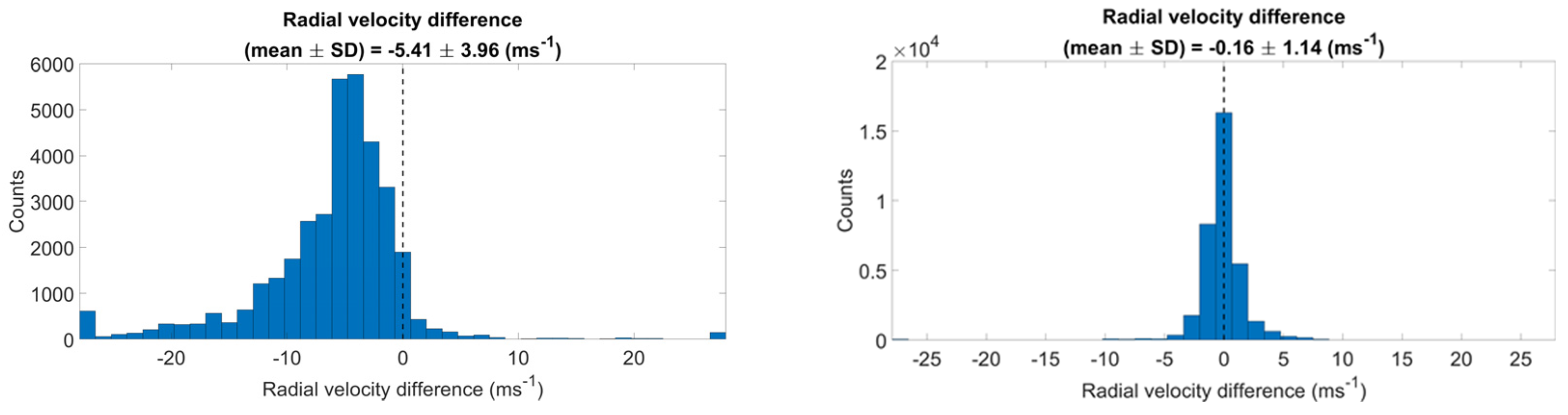
TLE/SGP4−5.413.96
SP−0.011.13
SP with ionospheric correction−0.020.86
ILRS−0.190.37
ILRS with ionospheric correction−0.050.24
Disclaimer/Publisher’s Note: The statements, opinions and data contained in all publications are solely those of the individual author(s) and contributor(s) and not of MDPI and/or the editor(s). MDPI and/or the editor(s) disclaim responsibility for any injury to people or property resulting from any ideas, methods, instructions or products referred to in the content.

