
Micro-Doppler Signature Analysis for Space Domain Awareness Using VHF Radar


Abstract
1. Introduction
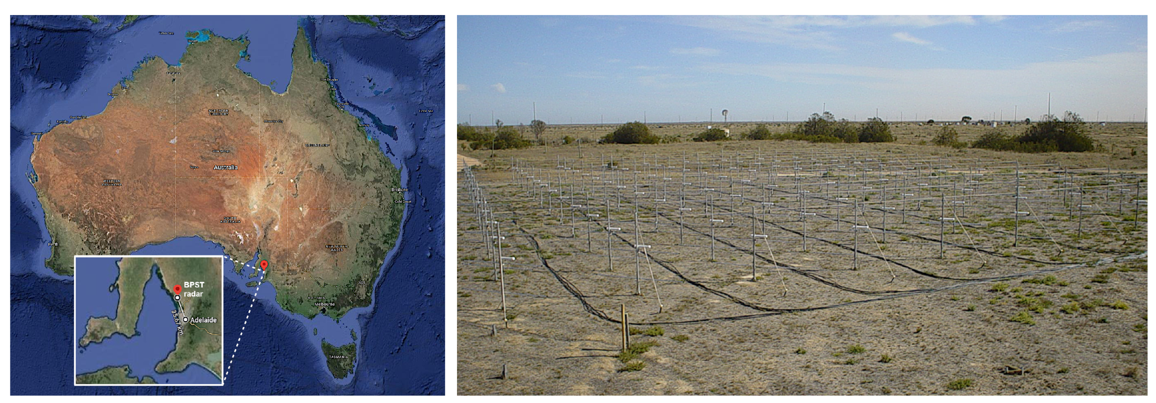
2. Buckland Park VHF Radar
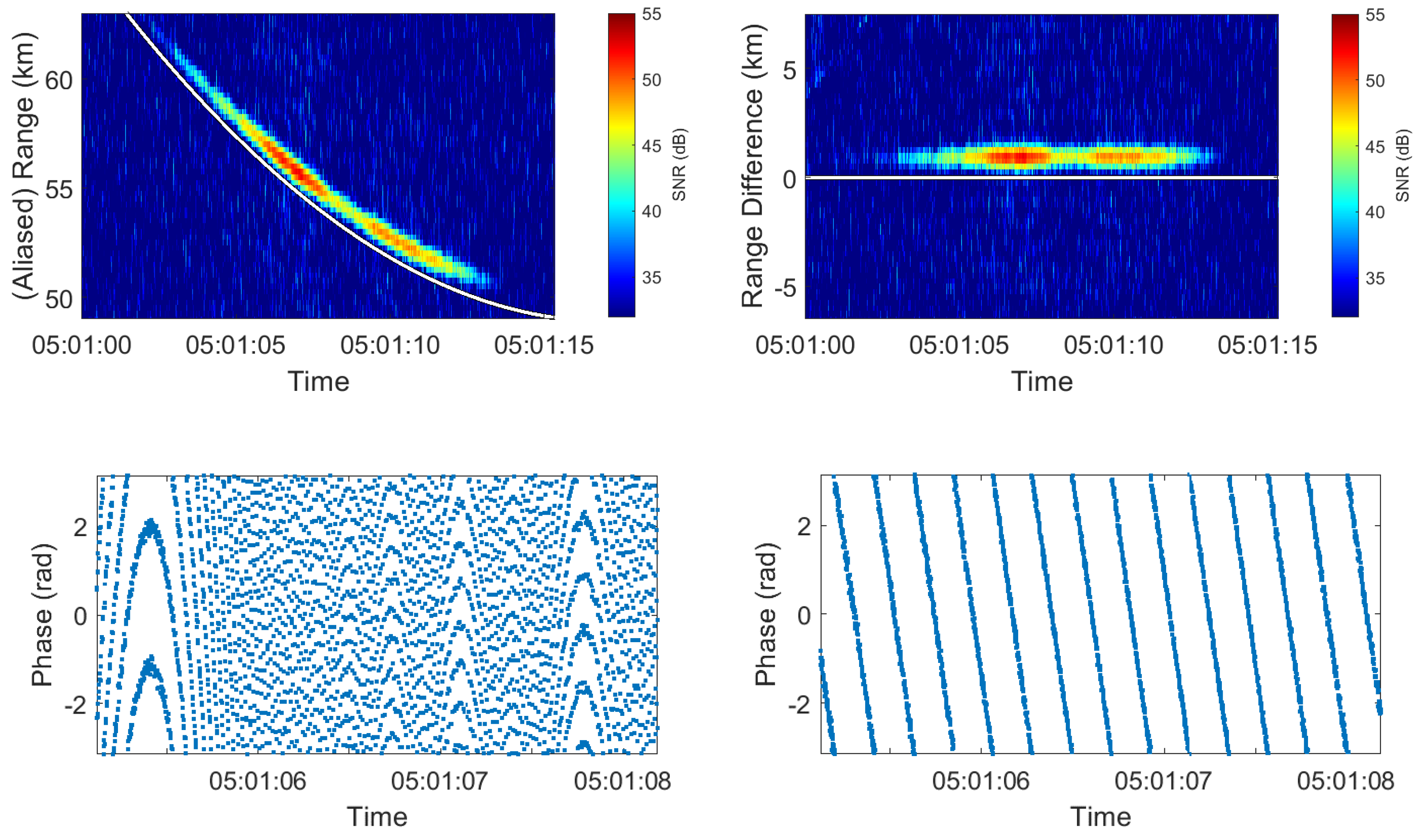
3. Automatic Translational Motion Compensation
- Range migration correction: The propagated range is used to convert the range–time data into “range-corrected” time data . This is achieved by interpolating in the range dimension similar to the technique used in the Keystone transform [23]. Alternatively, a circular shift can be performed on the data in the range dimension by samples, where represents the rounding up operator and is the range resolution. The latter option is feasible for the data presented in this paper as is oversampled by at least a factor of two.
- Phase correction: The “range-corrected” time data are then multiplied by a phase term based on the propagated range in (1) to compensate for phase differences introduced in step one.
4. Simulations
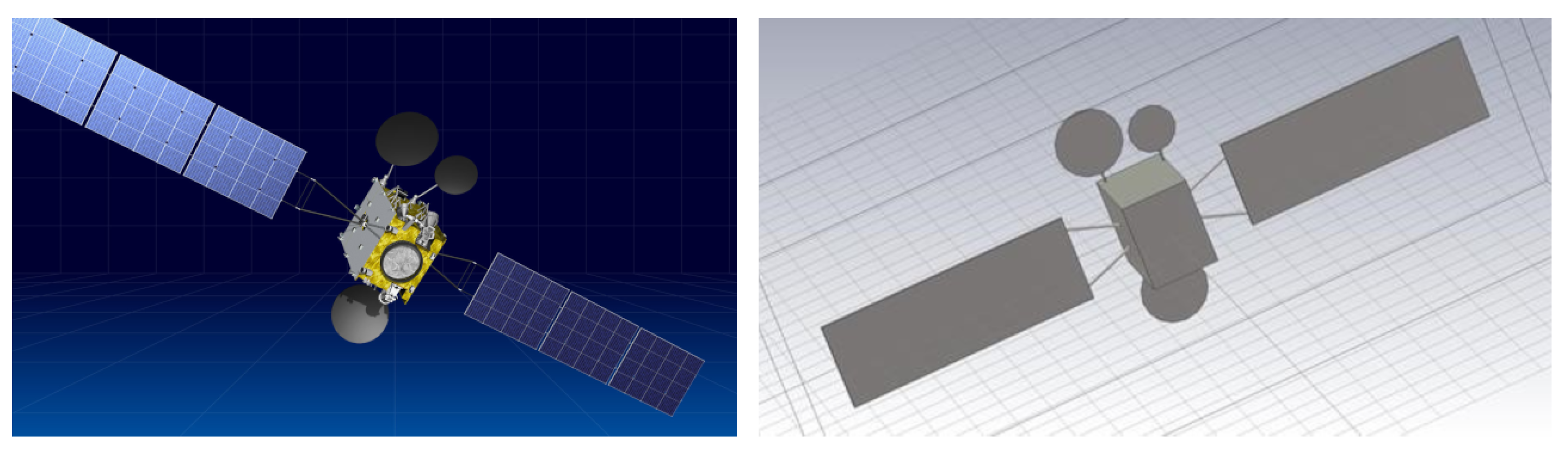
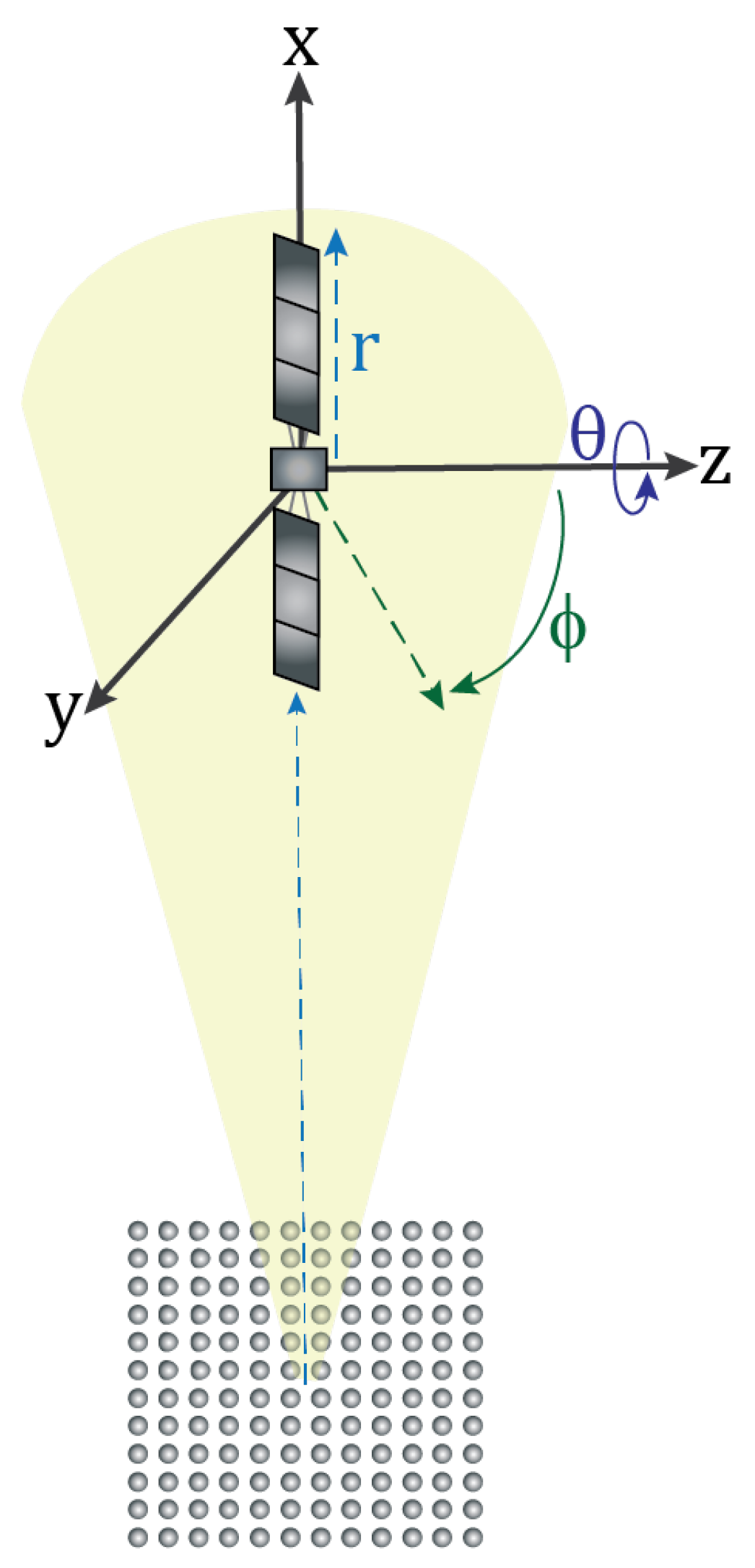
4.1. Satellite Information
4.2. Simulated Results
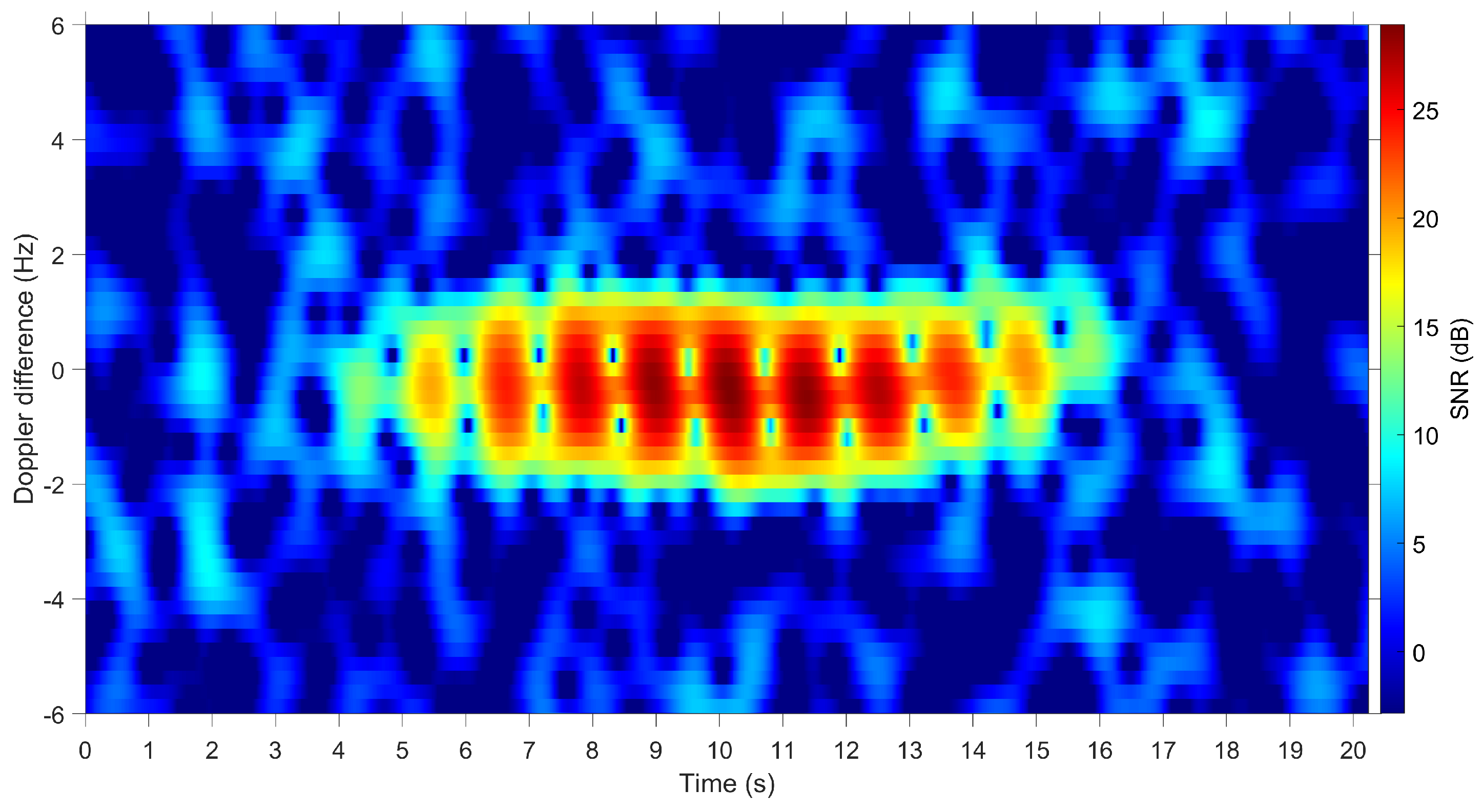
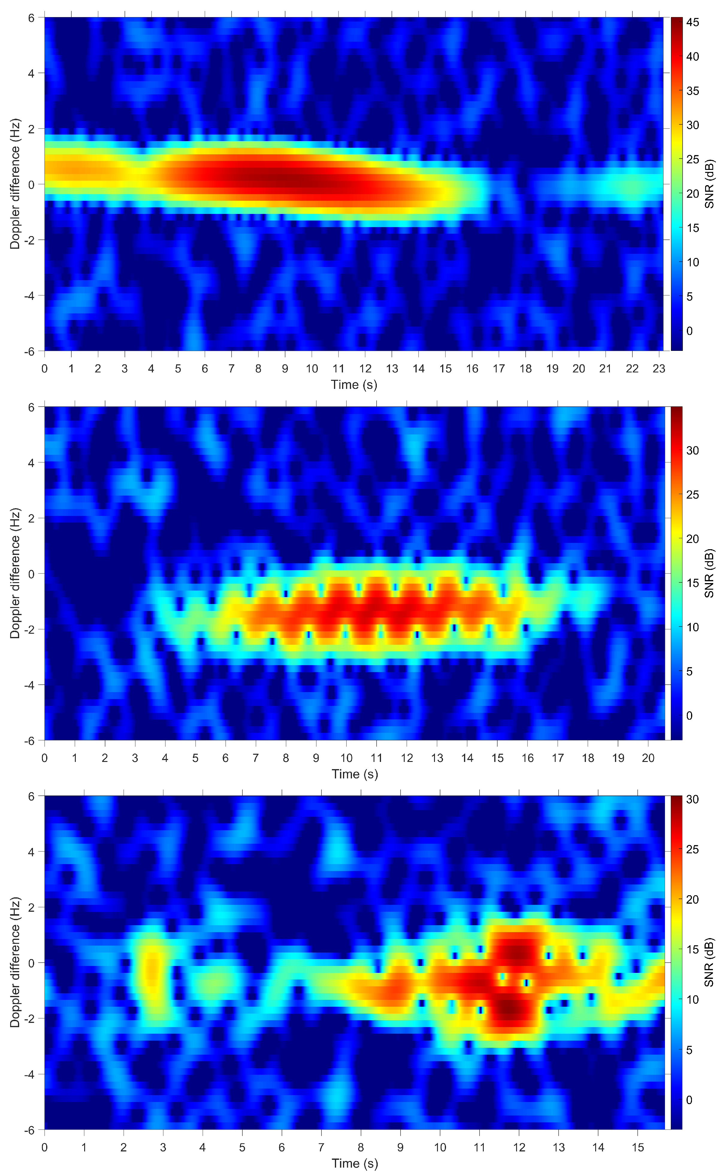
5. Micro-Doppler Signature Analysis
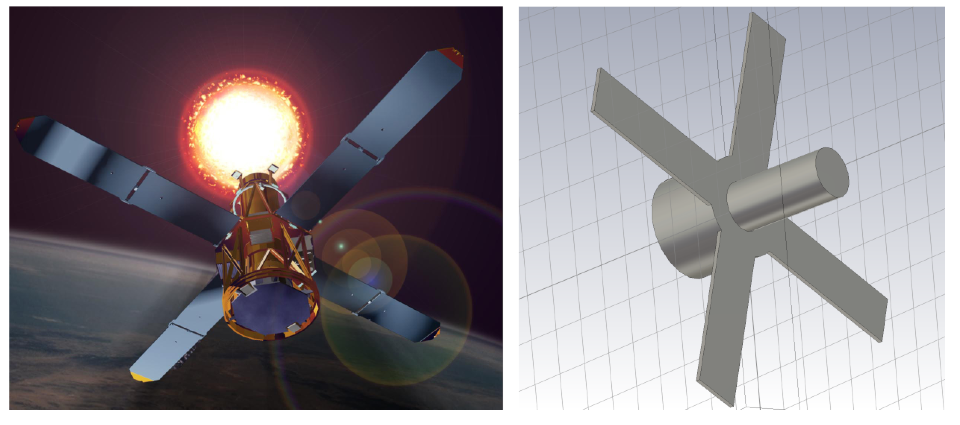
5.1. RHESSI
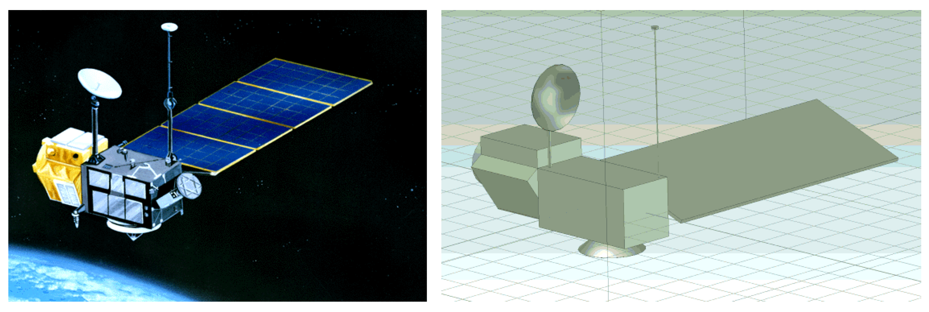
5.2. TOPEX/Poseidon
5.3. Telkom 3
6. Discussion
7. Conclusions
Author Contributions
Funding
Institutional Review Board Statement
Data Availability Statement
Acknowledgments
Conflicts of Interest
References
- Holdsworth, D.; Spargo, A.; Reid, I.; Adami, C. Low Earth Orbit object observations using the Buckland Park VHF radar. Radio Sci. 2020, 55, e2019RS006873. [Google Scholar] [CrossRef]
- Anger, S.; Anglberger, H.; Jirousek, M.; Dill, S.; Peichl, M. ISAR Imaging of Satellites in Space–Simulations and Measurements. In Proceedings of the 2019 20th International Radar Symposium (IRS), Ulm, Germany, 26–28 June 2019; pp. 1–6. [Google Scholar] [CrossRef]
- Hennessy, B.; Tingay, S.; Hancock, P.; Young, R.; Tremblay, S.; Wayth, R.B.; Morgan, J.; McSweeney, S.; Crosse, B.; Johnston-Hollitt, M.; et al. Improved Techniques for the Surveillance of the Near Earth Space Environment with the Murchison Widefield Array. In Proceedings of the IEEE Radar Conference, Boston, MA, USA, 22–26 April 2019. [Google Scholar]
- Palmer, J.E.; Hennessy, B.; Rutten, M.; Merrett, D.; Tingay, S.; Kaplan, D.; Ord, S.T.S.M.; Morgan, J.; Wayth, R.B. Surveillance of Space using passive radar and the Murchison Widefield Array. In Proceedings of the IEEE Radar Conference, Seattle, WA, USA, 8–12 May 2017. [Google Scholar]
- Smith, C.H.; Greene, B.; Bold, M.; Drury, R. Development of a new SSA facility at Learmonth Australia. In Proceedings of the Advanced Maui Optical and Space Surveillance Technologies Conference, Maui, HI, USA, 11–14 September 2018. [Google Scholar]
- Frazer, G.J.; Meehan, D.H.; Warne, G.M. Decametric measurements of the ISS using an experimental HF line-of-sight radar. In Proceedings of the 2013 International Conference on Radar, Adelaide, Australia, 9–12 September 2013. [Google Scholar]
- Frazer, G.J.; Rutten, M.; Cheung, B.; Cervera, M.A. Orbit determination using a decametric line-of-site radar. In Proceedings of the Advanced Maui Optical and Space Surveillance Technologies Conference (AMOS), Maui, HI, USA, 9–12 September 2014. [Google Scholar]
- Boley, A.; Byers, M. Satellite mega-constellations create risks in Low Earth Orbit, the atmosphere and on Earth. Sci. Rep. 2021, 11, 10642. [Google Scholar] [CrossRef] [PubMed]
- NASA Office of Inspector General Office of Audits. NASA’s Efforts to Mitigate the Risks Exposed by Orbital Debris; Technical Report IG-21-011; NASA: Washington, DA, USA, 2021. [Google Scholar]
- Nosrati, H.; Smith, S.; Hayman, D.; Horiuchi, S.; Hellicar, A. Bi-static Radar Interferometric Localization of MEO and GEO Space Debris using Australia Telescope Compact Array. In Proceedings of the Advanced Maui Optical and Space Technologies Conference, Maui, HI, USA, 27–30 September 2022. [Google Scholar]
- Heading, E.; Nguyen, S.; Holdsworth, D.; Field, D.; Reid, I. Analysis of RF Signatures for Space Domain Awareness using VHF radar. In Proceedings of the 2022 IEEE Radar Conference (RadarConf22), New York, NY, USA, 21–25 March 2022; pp. 1–6. [Google Scholar] [CrossRef]
- Benson, C.; Scheeres, D.; Moskovitz, N. Light-curves of Retired Geosynchronous Satellites. In Proceedings of the 76th European Conference on Space Debris, Darmstadt, Germany, 17–21 April 2017; Volume 7. [Google Scholar]
- Kudak, V.I.; Epishev, C.P.; Perig, V.M. Determining the orientation and spin period of TOPEX/Poseidon satellite by a photometric method. Astrophys. Bull. 2017, 72, 340–348. [Google Scholar] [CrossRef]
- Fulcoly, D.O.; Kalamaroff, K.I.; Chun, F.K. Determining Basic Satellite Shape from Photometric Light Curves. J. Spacecr. Rocket. 2012, 49, 76–82. [Google Scholar] [CrossRef]
- Eastment, J.D.; Ladd, D.N.; Walden, C.J.; Trethewey, M.L. Satellite observations using the Chibolton radar during the initial ESA ’CO-Vi’ tracking campaign. In Proceedings of the European Space Surveillance Conference, Madrid, Spain, 7–9 June 2011. [Google Scholar]
- Stevenson, M.; Nicolls, M.; Rosner, C. Space Object Attitude Stability Determined from Radar Cross-Section Statistics. In Proceedings of the Advanced Maui Optical and Space Surveillance Technologies Conference, Maui, HI, USA, 17–20 September 2019. [Google Scholar]
- Uysal, F.; van Dorp, P.; Serrano, A.; Kobsa, A.; Ghio, S.; Kintz, A.; Bassa, C.; Garrington, S.; Caro Cuenca, M.; Otten, M.; et al. Large Baseline Bistatic Radar Imaging for Space Domain Awareness. In Proceedings of the Radar 2023, Berlin, Germany, 20–22 September 2023. [Google Scholar]
- Ghio, S.; Martorella, M. Estimation of rotating RSO parameters using radar data and joint time-frequency transforms. In Proceedings of the 7th European Conference on Space Debris, Darmstadt, Germany, 18–21 April 2017. [Google Scholar]
- Jung, K.; Lee, J.I.; Kim, N.; Oh, S.; Seo, D.W. Classification of Space Objects by using Deep Learning with Micro Doppler Signature Images. Sensors 2021, 21, 4365. [Google Scholar] [CrossRef] [PubMed]
- Cammenga, Z.A.; Baker, C.J.; Smith, G.E.; Ewing, R. Micro-Doppler target scattering. In Proceedings of the 2014 IEEE Radar Conference, Cincinnati, OH, USA, 9–23 May 2014; pp. 1451–1455. [Google Scholar] [CrossRef]
- Dolman, B.; Reid, I.; Tingwell, C. Stratospheric tropospheric wind profiling radars in the Australian network. Earth Planets Space 2018, 70, 170. [Google Scholar] [CrossRef]
- Adelaide, T.U. Buckland Park VHF ST Radar. 2024. Available online: http://www.physics.adelaide.edu.au/atmospheric/vhf.html (accessed on 1 February 2024).
- Richards, M. The keystone transformation for correcting range migration in range-doppler processing. Pulse 2014, 1000, 13–14. [Google Scholar]
- Lin, R.P.; Dennis, B.R.; Hurford, G.J.; Smith, D.M.; Zehnder, A.; Harvey, P.R.; Conway, A. The Reuven Ramaty High-Energy Solar Spectroscopic Imager (RHESSI); Springer: Dordrecht, The Netherlands, 2003. [Google Scholar]
- Krebs, G.D. RHESSI (RHESSI, Reuven Ramaty, SMEX 6, Explorer 81). 2023. Available online: https://space.skyrocket.de/doc_sdat/explorer_hessi.htm (accessed on 1 February 2024).
- Hill, D. NASA Retired Solar Energy Imager Spacecraft Reenters Atmosphere. 2023. Available online: https://www.nasa.gov/feature/nasa-retired-solar-energy-imager-spacecraft-reenters-atmosphere (accessed on 1 February 2024).
- Dennis, B. RHESSI MISSION FACTS. 2023. Available online: https://hesperia.gsfc.nasa.gov/rhessi2/mission/mission-facts/index.html (accessed on 1 February 2024).
- NASA. TOPEX/Poseidon. 2021. Available online: https://sealevel.jpl.nasa.gov/system/documents/files/1674_tp-fact-sheet.pdf (accessed on 1 February 2024).
- Page, G.S. Telkom 3. 2021. Available online: https://space.skyrocket.de/doc$_$sdat/telkom-3.htm (accessed on 1 February 2024).
- Technology, A. Telkom-3 Communications Satellite, Indonesia. 2021. Available online: https://www.aerospace-technology.com/projects/telkom3-communication-satellite-indonesia (accessed on 1 February 2024).
- Reshetnev, J.A.M. Information Satellite Systems. 2021. Available online: http://www.iss-reshetnev.com/spacecraft/spacecraft-communications/telkom-3 (accessed on 1 February 2022).
- Munson, D.; O’Brien, J.; Jenkins, W. A tomographic formulation of spotlight mode synthetic aperture radar. Proc. IEEE 1983, 71, 917–925. [Google Scholar] [CrossRef]
- Tran, H.T.; Heading, E.; Ng, B.H. On the Slow-Time k-Space and its Augmentation in Doppler Radar Tomography. Sensors 2020, 20, 513. [Google Scholar] [CrossRef] [PubMed]
- Klobuchar, J. Ionospheric Effects on Earth-Space Propagation; Technical Report AFGL-TR-84-0004; Ionospheric Physics Division: Air Force Geophysics Laboratory: Bedford, MA, USA, 1983. [Google Scholar]


| PRF | 2 kHz |
| No. Coherent Averages | 2 |
| Temporal Sampling Frequency | 1 kHz |
| Waveform | 13-bit Barker code |
| Baud Length | km |
| Pulse Length | km |
| Receive Filter Width | 64 kHz |
| Range Resolution | km |
| Object Feature | RHESSI | TOPEX/Poseidon | Telkom 3 |
|---|---|---|---|
| No. Solar Panels | 4 | 1 | 2 |
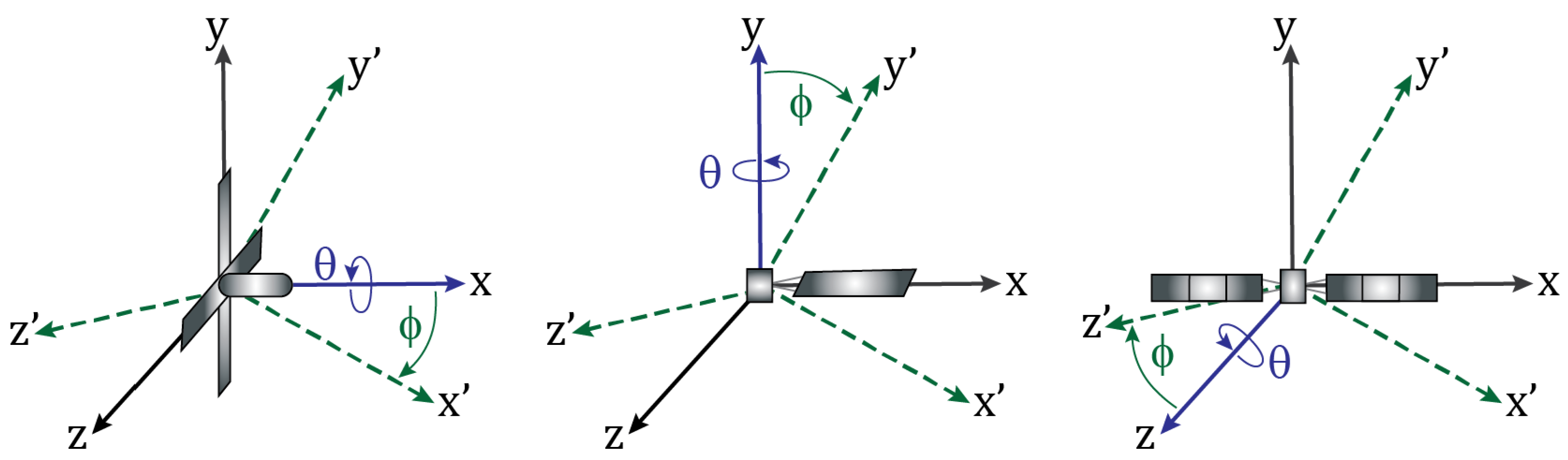
| Spin Axis | x | y | z |
| Elevation Angle | |||
| Polarisation | V | V | V |
| Object Feature | RHESSI | TOPEX/Poseidon | Telkom 3 |
|---|---|---|---|
| Estimated Doppler Extent | Hz | 3 Hz | 4 Hz |
| Estimated Rotation Period | s | 11 s | s |
| Estimated Rotation Rate | rad/s | rad/s | rad/s |
| Estimated Length | m | m | m |
| True Length | m | m | 23 m |
Disclaimer/Publisher’s Note: The statements, opinions and data contained in all publications are solely those of the individual author(s) and contributor(s) and not of MDPI and/or the editor(s). MDPI and/or the editor(s) disclaim responsibility for any injury to people or property resulting from any ideas, methods, instructions or products referred to in the content. |
© 2024 by the authors. Licensee MDPI, Basel, Switzerland. This article is an open access article distributed under the terms and conditions of the Creative Commons Attribution (CC BY) license (https://creativecommons.org/licenses/by/4.0/).
Share and Cite
Heading, E.; Nguyen, S.T.; Holdsworth, D.; Reid, I.M. Micro-Doppler Signature Analysis for Space Domain Awareness Using VHF Radar. Remote Sens. 2024, 16, 1354. https://doi.org/10.3390/rs16081354
Heading E, Nguyen ST, Holdsworth D, Reid IM. Micro-Doppler Signature Analysis for Space Domain Awareness Using VHF Radar. Remote Sensing. 2024; 16(8):1354. https://doi.org/10.3390/rs16081354
Chicago/Turabian StyleHeading, Emma, Si Tran Nguyen, David Holdsworth, and Iain M. Reid. 2024. "Micro-Doppler Signature Analysis for Space Domain Awareness Using VHF Radar" Remote Sensing 16, no. 8: 1354. https://doi.org/10.3390/rs16081354
APA StyleHeading, E., Nguyen, S. T., Holdsworth, D., & Reid, I. M. (2024). Micro-Doppler Signature Analysis for Space Domain Awareness Using VHF Radar. Remote Sensing, 16(8), 1354. https://doi.org/10.3390/rs16081354