Mapping of Forest Structural Parameters in Tianshan Mountain Using Bayesian-Random Forest Model, Synthetic Aperture Radar Sentinel-1A, and Sentinel-2 Imagery

Abstract

The assessment of forest structural parameters is crucial for understanding carbon storage, habitat suitability, and timber stock. However, the labor-intensive and expensive nature of field measurements, coupled with inadequate sample sizes for large-scale modeling, poses challenges. To address the forest structure parameters in the Western Tianshan Mountains, this study used UAV-LiDAR to gather extensive sample data. This approach was enhanced by integrating Sentinel satellite and topographic data and using a Bayesian-Random Forest model to estimate forest canopy height, average height, density, and aboveground biomass (AGB). Validation against independent LiDAR-derived samples confirmed the model’s high accuracy, with coefficients of determination (R²) and root mean square errors (RMSE) indicating strong predictive performance (R² = 0.63, RMSE = 5.06 m for canopy height; R² = 0.64, RMSE = 2.88 m for average height; R² = 0.68, RMSE = 62.84 for density; and R² = 0.59, RMSE = 29.71 Mg/ha for AGB). Notably, the crucial factors include DEM, Sentinel-1 (VH and VV backscatter in dB), and Sentinel-2 (B6, B8A, and B11 bands). These factors contribute significantly to the modeling of forest structure. This technology aims to expedite and economize forest surveys while augmenting the range of forest parameters, especially in remote and rugged terrains. Using a wealth of UAV-LiDAR data, this outcome surpasses its counterparts’ by providing essential insights for exploring climate change effects on Central Asian forests, facilitating precise carbon stock quantification, and enhancing knowledge of forest ecosystems.

1. Introduction

The Tianshan forests are essential for preserving the ecological balance among oasis, desert, and forest ecosystems. They regulate the climate cycle, conserve soil and water, protect biodiversity, sequester carbon, and support the timber economy [1]. However, the forests are facing challenges due to fluctuating climate change, including prolonged extreme droughts and rising temperatures [2,3]. Conducting a survey to assess the current state of the forests is imperative to address these impacts and implement conservation measures.

Forest canopy height, average height, density, and aboveground biomass (AGB) are key indicators of forest ecosystem structure and biodiversity [4,5,6]. However, due to the complex topography and steep slopes of the region, manual data collection and instrumental measurements face challenges and accuracy issues. Presently, most available results are based on large-scale simulations or small forest surveys, lacking a complete representation of the natural forests in Tianshan. To address this, it is necessary to redesign sampling sites to better reflect the characteristics of forests, thereby improving the precision of forest structure parameter simulations and gaining a more comprehensive understanding of the forest ecosystem in this region.

The accuracy of mapping products in remote sensing applications heavily relies on the quantity and quality of training data [7,8]. However, gathering ground reference data has limitations, such as the quantity being constrained by time-consuming and expensive fieldwork. Long-established forest inventories provide valuable data but lack the spatial information at the local and regional scales required for effective forest management in the context of climate change challenges. Moreover, ground-based observations face challenges such as dense canopy cover, accessibility, and representativeness, making it difficult to establish statistical links with satellite observations taken from above the canopy. The discrete nature of field data also poses difficulties in matching them with continuous earth observation data at various spatial scales.

To overcome these limitations, this study proposes the use of unmanned aerial vehicles (UAVs) as a source of reference data collection. UAV-based remote sensing can obtain spatially continuous information on species coverage at very high spatial resolution [9,10,11]. The application of UAV data instead of in-situ data has several advantages: (1) increased data quantity can be obtained in each timeframe, (2) data collection is not impeded by accessibility (e.g., topography) and is therefore more representative, (3) UAV data have the same viewing angle as satellite data, and (4) descriptions of target species from UAV-collected data can be leveraged with automated algorithms to enhance the efficiency of reference data collection [12]. However, UAV data still have limitations when it comes to characterizing large-scale forests, and the significant time and economic costs of acquiring them cannot be ignored.

Satellite systems are essential for forest monitoring, especially when UAV-LiDAR resources are limited or analysis requires regional/global scale [13,14]. Satellites offer global remote sensing data, ensuring consistency across different geographical areas and enabling long-term monitoring of forest structural parameters. High-resolution satellites, like Sentinel missions, provide detailed forest characteristics for small-scale studies, local forest management, and environmental sensitivity analyses [15]. Sentinel multiple spectral bands, including visible, infrared, and microwave, allow estimation of forest biomass, chlorophyll content, and vegetation cover [16,17]. Sentinel Synthetic Aperture Radar (SAR) complements optical sensors, providing all-weather, day-and-night visibility and retrieving surface roughness like vegetation density and forest species [18,19].

Machine learning combined with remote sensing image data has been widely used to simulate forest structural parameters, encompassing both classification and regression, which have certain advantages [16,20]. Machine learning can effectively deal with large-scale, complex data through automated feature selection, model tuning, and prediction. The most common and widely used machine learning methods are decision trees (e.g., random forest) and support vector machines. Random Forest (RF), a prominent machine learning approach based on integrated learning, conducts classification and regression analyses by constructing multiple decision tree models and aggregating their predictions. Notably, RF demonstrates robustness against noisy data and overfitting while being adaptable to diverse data distributions and feature relationships. It provides feature importance analysis, quantifying the contributions of features used in decision tree construction. Furthermore, RF excels at handling high-dimensional and large-scale datasets, effectively managing data with numerous features and samples, and mitigating dimensionality issues [21,22,23].

This study employed the Bayesian-Random Forest model to assess the capabilities of Sentinel-1 and -2 series data, along with DEM data, for modeling forest structural parameters. To train and validate predictive models, UAV-LiDAR data were used as real-world data. The objectives of this study were to (1) demonstrate the adaptability of the Bayesian-Random Forest model in accurately predicting forest structural parameters; (2) investigate the potential of Sentinel-1, Sentinel-2, and DEM data in predicting forest structural parameters in the Tianshan Mountains; and (3) explore the spatial distribution characteristics of forest canopy height (m), average height (m), density (plant/ha), and AGB (t/ha) in the western Tianshan Mountains.

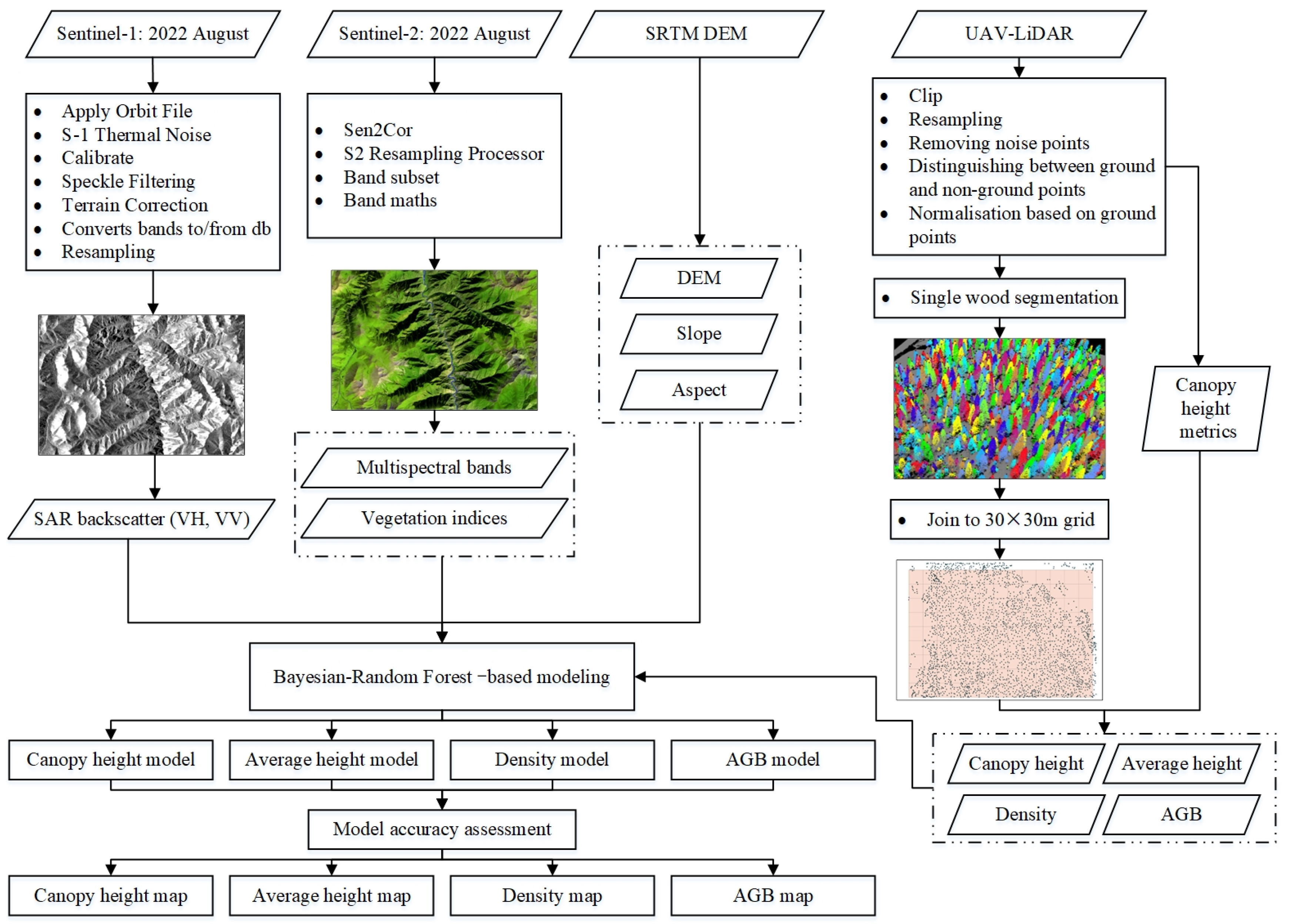
2. Materials and Methods

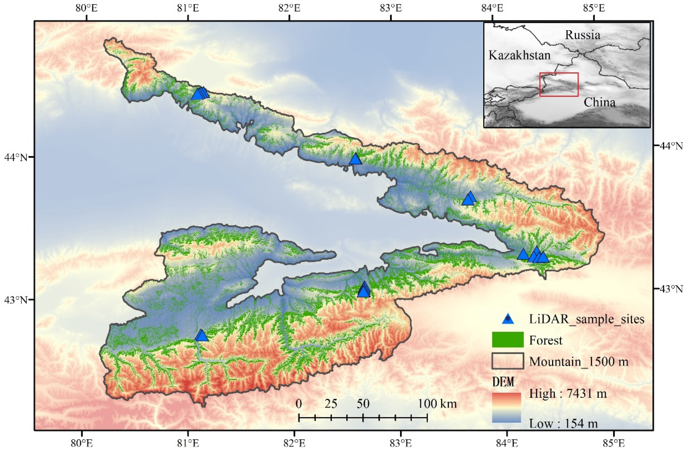
2.1. Study Region

The study area is in the Western Tianshan Mountains (Figure 1), which is characterized by an arid and semi-arid climate and is the source of several international rivers. The forest on the northern slopes of Tianshan Mountain is predominantly composed of shade- and drought-tolerant Schrenk spruces (Picea schrenkiana). These forests primarily thrive in regions with mild climates, fertile soils, and ample rainfall. The average annual temperature within the distribution area ranges from 3 to 5 °C, with an annual precipitation of 400 to 700 mm. During summer, the relative humidity of the atmosphere exceeds 64%, and the average temperature of the hottest month ranges between 10 and 12 °C (lower limit) and 16 and 18 °C (upper limit) [24]. Mature forests in the area exhibit an average tree height above 30 m, reaching heights of up to 60 m. Their diameter at breast height (DBH) ranges from 40 cm to a maximum of 1.5 m, with a characteristic straight and rounded stem shape [25].

The sampling sites were uniformly distributed in the study area, and at the same sampling site, sample plots distributed at different altitudes were set up to ensure the collection of forest structural parameters at different altitudes (Figure 1). The metrics used to characterize the structural parameters of the forest in this area were: forest canopy height (m), average height (m), density (plant/ha), and above-grand biomass (AGB) (t/ha). We defined forest canopy height as the 95th height percentile in a 30 m × 30 m plot; forest average height as the mean of all tree heights in a 30 m × 30 m plot; density as the number of trees per unit area; and forest AGB as the SUM of aboveground biomass of all trees per unit area, which was obtained based on the height of each tree. The equation used was as follows [26]:

$$W=0.0641H^{2.854}$$

(1)

$$AGB={\sum }_{i=1}^n{W}_i$$

(2)

where H represents the height of a single tree, W represents the aboveground biomass of a single tree, i represents the ith tree in the sample plot, and n represents the number of trees in the sample plot.

The comprehensive framework for data processing and model development is illustrated in Figure 2.

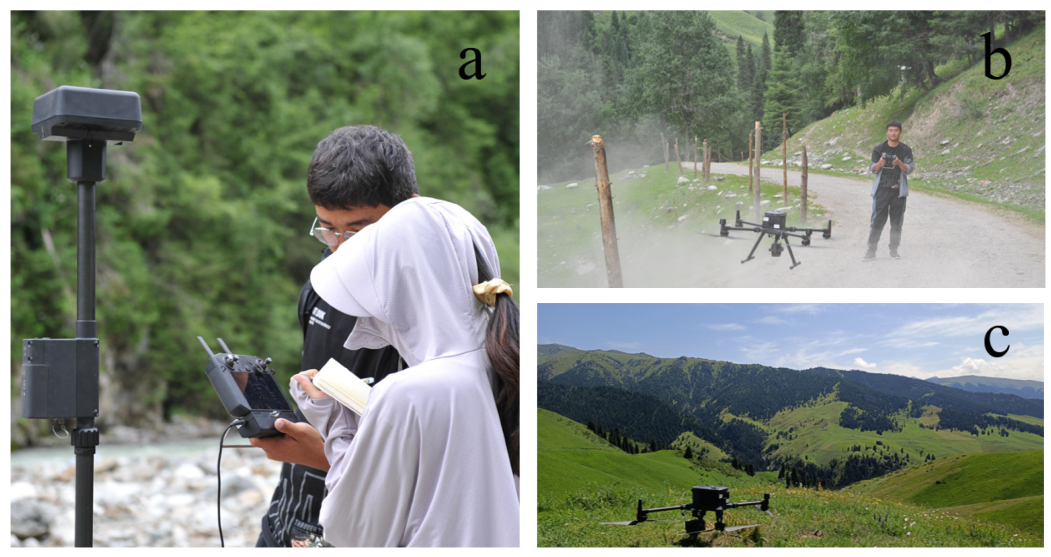
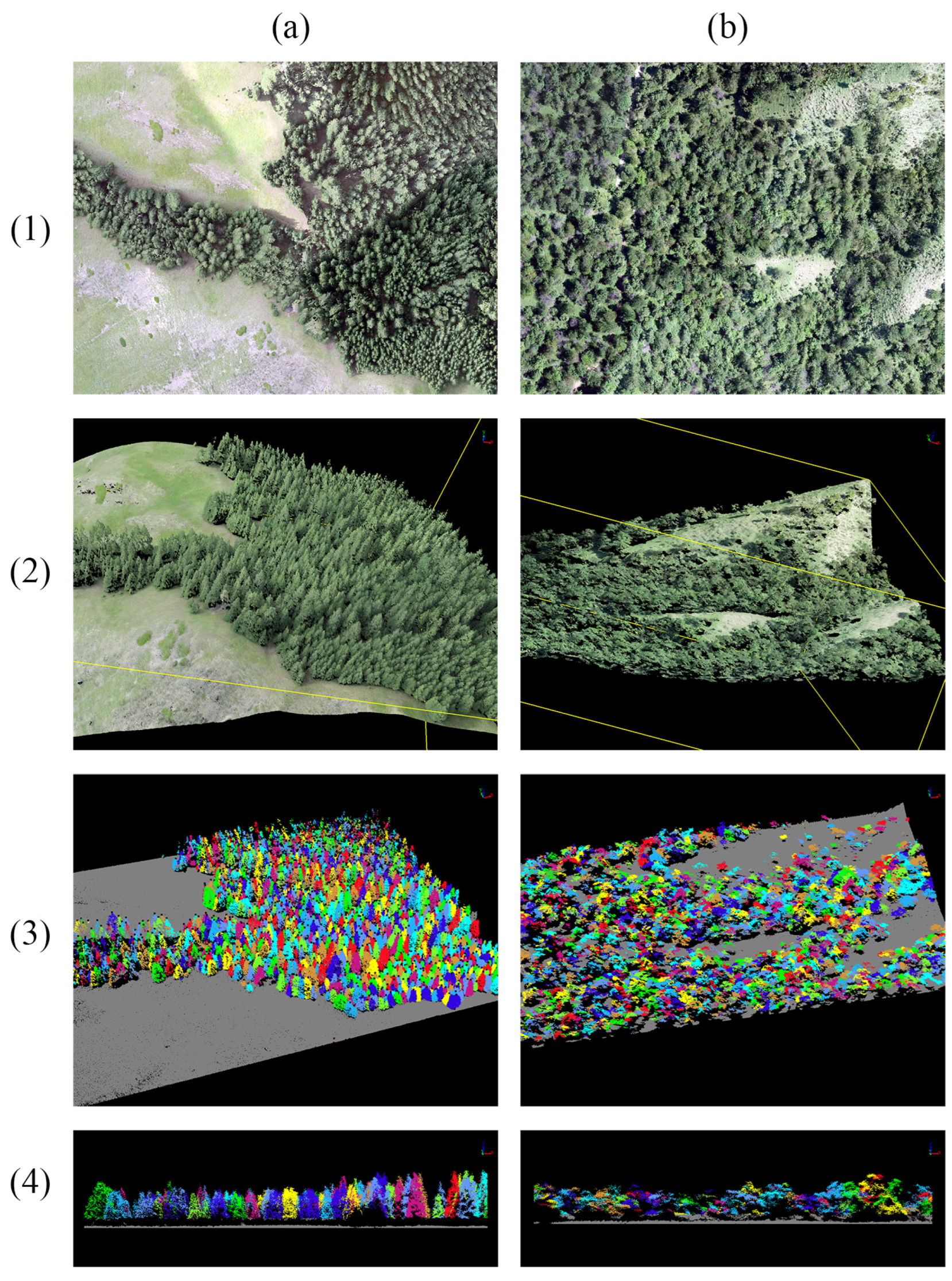
2.2. UAV-LiDAR Data

In July 2022, we conducted UAV LiDAR data acquisition using the L1 sensor mounted on a DJI M300 UAV (Figure 3). The data acquisition parameters were configured as follows: the echo mode was set to dual echo, the sampling frequency was selected as 240 KHz, and the UAV maintained a course speed of 8 m/s, and a point cloud density > 200 points/m². Furthermore, we established a laser overlap of 60% to guarantee adequate coverage. The relative height between the UAV’s course height and the ground was maintained within the range of 50 to 200 m. These specific parameters were chosen to optimize the data collection process and enhance the quality of the acquired LiDAR data. The LiDAR data were georeferenced using the WGS 84/UTM zone 44 N coordinate system. This allowed us to proceed with detailed analysis and exploration of the dataset.

In this study, the LiDAR data in LAS format was imported into LiDAR360 6.0 software developed by GreenValley, Beijing, China (https://www.greenvalleyintl.com/LiDAR360/, (accessed on 31 May 2023)). Pre-processing steps were performed, including cropping areas with incomplete edge point clouds, resampling, denoising, ground point classification, and normalization based on ground points. Forest parameters, such as height metrics, were calculated using a grid-based approach. In addition, single tree segmentation was used to obtain latitude, longitude, height, and canopy data for all single trees in the sample plots. ArcGIS 10.5 software was used to join the single-tree segmentation data to 30 m × 30 m grids to calculate the number of trees and the average height on each grid. Based on the height of the tree, the AGB of all the individual trees on the grids was calculated using Equation (1), and subsequently, the sum of the AGB on each grid was calculated using Equation (2). The above process acquires four variables: forest canopy height, average height, density, and AGB with a resolution of 30 m.

For this, 163.35 ha of LiDAR data were used for model training, which came from 25 sample plots of 400 m × 400 m, and a total of 1815 samples were used for statistical analysis and model training.

2.3. Topography (DEM)

The digital elevation model (DEM) data used in this study was obtained from the Shuttle Radar Topography Mission (SRTM). SRTM employed a multibeam radar system capable of capturing high-quality elevation data. To derive slope and aspect information, the DEM data were processed using ArcGIS 10.5 software. The SRTM-generated DEM data had a spatial resolution of 30 m, encompassing the study area. The data were downloaded from the United States Geological Survey’s Earth Explorer platform (https://earthexplorer.usgs.gov/, (accessed on 15 March 2023)).

2.4. Sentinel Image Data

This study used data from Sentinel-1 (Synthetic Aperture Radar) and Sentinel-2 (Multispectral) imagery, which were acquired from the European Space Agency and downloaded from the Copernicus Open Access Hub (https://scihub.copernicus.eu/dhus/#/home, (accessed on 20 March 2023)). All pre-processing steps were performed using the SNAP 9.0.0 software, which is specifically designed for processing and analyzing satellite data.

The Sentinel-1 C-band (5.405 GHz) images used in this study were collected in Interferometric Wide Swath mode with VH (Vertical transmit–Horizontal receive) and VV (Vertical transmit–Vertical receive) polarizations. They were processed to a high-resolution Level-1 Ground Range Detected (GRD) level, already multi-looked (5 × 1) with a pixel size of 10 m. Preprocessing in SNAP 9.0.0 software involved steps such as orbit file application, thermal noise removal, radar calibration, speckle filtering, terrain correction, conversion to/from dB, and resampling to a 30 m × 30 m pixel size. These processing steps resulted in backscatter coefficient data, providing valuable information about surface parameters such as geometry, dielectric properties, and roughness.

The Sentinel-2 data used in this study is a Level 1C product consisting of orthorectified, top-of-atmosphere reflectance imagery. It covers a 100 km by 100 km area in UTM/WGS 84 projection and includes 13 spectral bands spanning the visible, near infrared, and short-wave infrared regions. The spatial resolutions vary, with 10 m (4 bands), 20 m (6 bands), and 60 m (3 bands) options available. We chose multiple bands that are sensitive to reflections from vegetation. The Level-1C data underwent atmospheric correction using the Sen2Cor (version 02.11.00) processor, based on the radiative transfer model. The resulting Level-2A products were then converted to this study’s common map projection of WGS 84/UTM zone 44 N and resampled to a 30 m pixel size. The vegetation indices listed in

Table 1. The list of indices for predicting in this study.

Source Image	Predictor Variable	Relevant Channel/Band/Index	Definition
SRTM	Topographic features	DEM, slope, and aspect	/
Sentinel-1	Polarization/channel	Sentinel1_1 and sentinel1_2	VH and VV backscatter in dB
Sentinel-2	Multispectral bands	B4, B5, B6, B7, B8, B8A, B11, and B12	/
	Vegetation indices	NDVI	(B8 − B4)/(B8 + B4)

were calculated using band math. In the final analysis, multiple single bands and vegetation indices were obtained from the Sentinel-2 imagery.

2.5. Machine Learning Algorithm

A Bayesian optimizer was employed to optimize a random forest regression model (RF) that integrated LiDAR-based forest structural parameters with predictor variables. A total of 14 predictor variables were added to the model during training. The predicted forest structural parameters included forest canopy height, average height, density, and AGB.

2.5.1. Random Forest Regression Model with Bayesian Optimization

The random forest regression model (RF) is an effective and versatile integrated learning method used for regression problems [27]. It is based on decision tree algorithms and combines multiple decision trees to make predictions. This model is particularly suitable for datasets with numerous features and intricate relationships, as it exhibits robustness and high prediction performance. Moreover, the random forest model demonstrates strong resilience against outliers and noise, requiring minimal data pre-processing. Its wide applicability and ability to handle complex datasets make it a popular choice in many research studies [28,29,30].

A Bayesian optimizer was employed to fine-tune the model parameters. The Bayesian optimizer effectively improves the objective function value by iteratively selecting the next parameter point, leading to the identification of the best parameter combination within a finite number of iterations. Compared to traditional grid search or stochastic search methods, Bayesian optimizers converge to the optimal solution more efficiently, resulting in faster and more effective parameter tuning [31,32].

The models used an 80/20 train-test split, with 80% of the samples (N = 1452) used for training and 20% for validation (N = 363). To reduce the dimensionality of the data and identify the most informative variables, an importance analysis was conducted using the RF model. Recursive feature elimination and cross-validation based on the ordering of predictor importance were implemented to select a subset of predictors that would facilitate the best predictions. A RF-based predictive model was then built using these selected variables. This approach ensured the inclusion of the most relevant variables while reducing the complexity of the model and improving its predictive performance.

All data processing and model simulations were conducted in Python 3.10, using libraries such as BayesOpt and scikit-learn [33,34].

2.5.2. Accuracy Assessment

To assess the performance of the predictive model for the specific regression problem, a comprehensive evaluation of the prediction results was conducted. This evaluation was essential in determining the reliability and suitability of the model, as well as identifying areas for improvement or alternative model selection. Multiple metrics were employed, including root mean square error (RMSE), BIAS, coefficient of determination (R²), and scatterplot analysis between predicted and measured values. These evaluation metrics provided insights into the accuracy and precision of the model’s predictions.

$$RMSE=\sqrt{\frac{{\sum }_i{\left(y_i-{\widehat{y}}_i\right)}^2}{n}}$$

$$R^2=1-\frac{S{S}_{res}}{S{S}_{tot}}=1-\frac{{\sum }_i{\left(y_i-{\widehat{y}}_i\right)}^2}{{\sum }_i{\left(y_i-{\overline{y}}_i\right)}^2}$$

$$Bias=\frac{1}{n}{\displaystyle \sum }_{i=1}^n\left(y_i-{\widehat{y}}_i\right)$$

where $y_i$ is the measured value for the i-th data point from LiDAR data, ${\widehat{y}}_i$ is the predicted value for the i-th data point, and $n$ is the total number of measurements.

Additionally, we compared them with those obtained from other studies or models. Four sample plots were randomly selected and compared with the sliding average of forest canopy height estimated by our model and others with that measured by UAV-LiDAR. Both training and validation data were present in these sample plots. The aim was to confirm which model-simulated forest canopy heights were closer to those interpreted by LiDAR. We conducted a visual comparison of canopy heights estimated by our model and other models with Google Earth images. This comparison served two purposes: first, to illustrate the variations in simulation outcomes across different models, and second, to highlight how each model distinguishes forest boundaries. These sample plots for this comparison were selected randomly in the study area.

3. Results

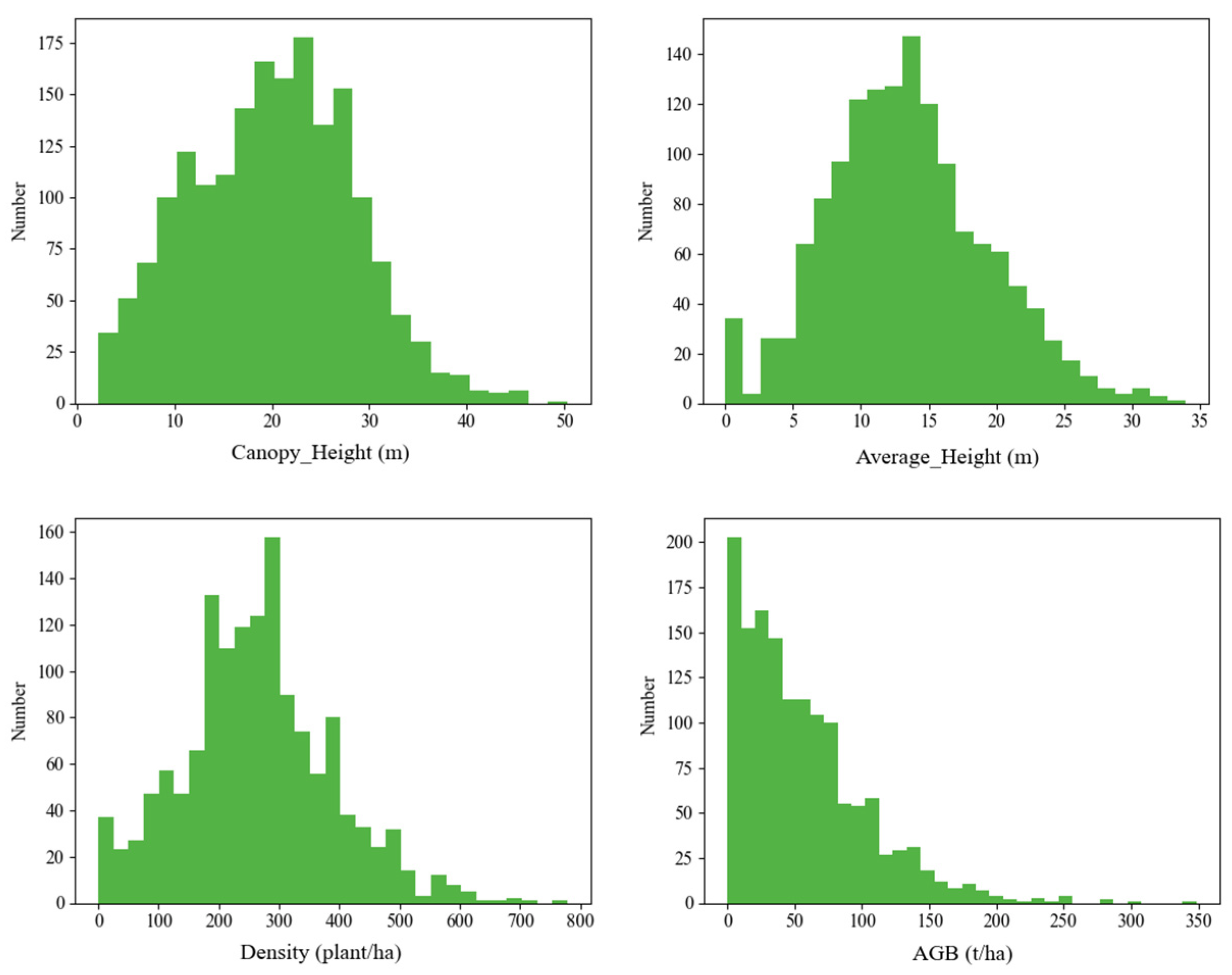
3.1. LiDAR-Derived Forest Structure Parameters

Figure 4 illustrates the results of the measurements from the LiDAR data for the forest structural parameters. The maximum forest canopy height was 50.3 m, with a mean of 20.1 m; the maximum forest average height was 34.0 m, with a mean of 13.4 m; the maximum forest density was 778 trees per hectare, and a mean was 264 trees per hectare; and the maximum AGB was 348.5 t/ha, and the mean was 56.3 t/ha.

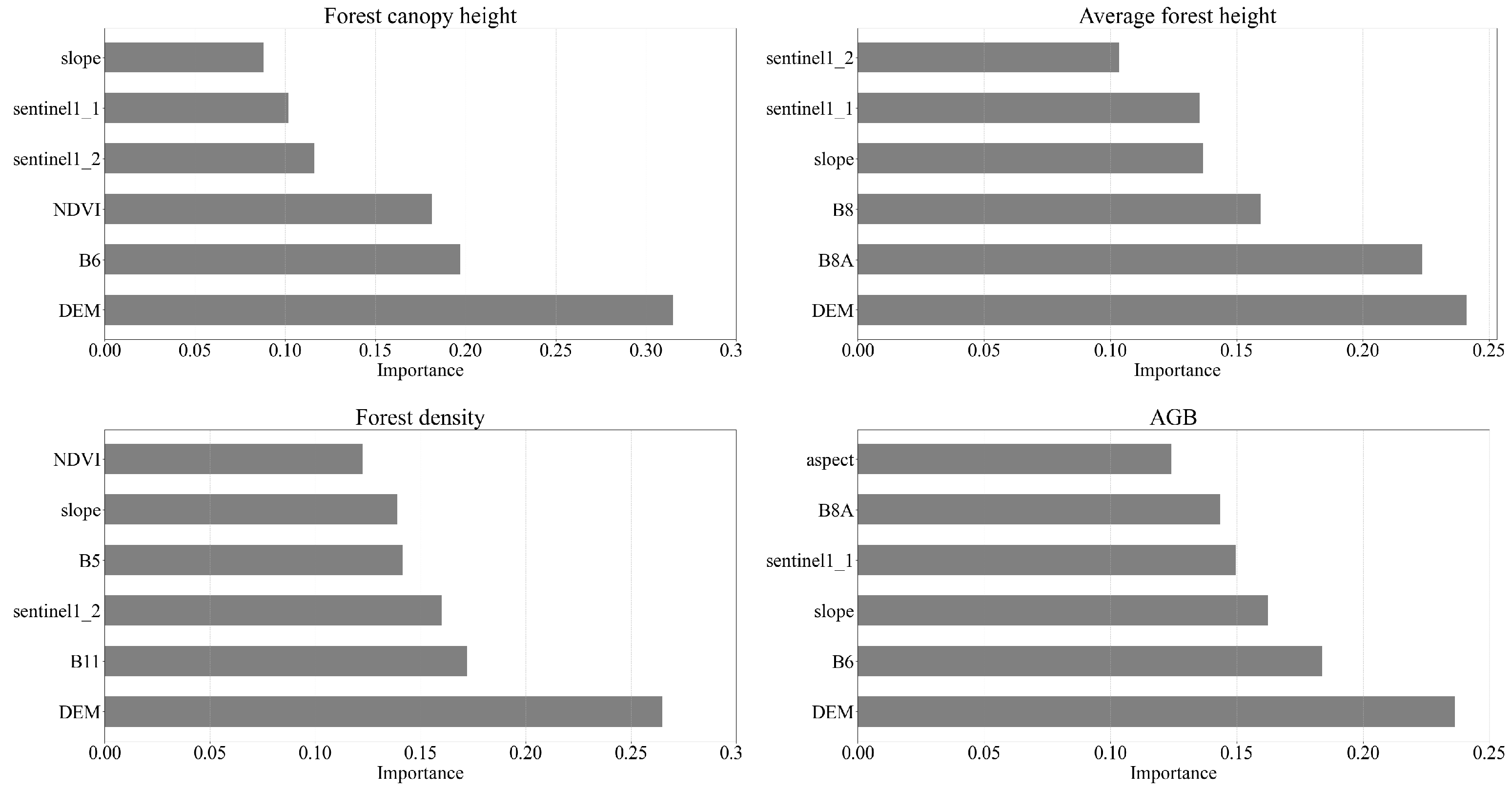
3.2. Predictor Variable Selection

To assess variable contributions in the predictive model, the Bayesian-Random Forest algorithm has been employed for optimal parameterization. Using the variable importance module, the top 6 variables were ranked and selected from 14 variables. Figure 5 illustrates the importance of these variables in different forest structural parameter estimation models, each with a unique variable combination.

Figure 5 illustrates how the forest canopy height model identified DEM as the variable with the greatest influence, followed by B6, NDVI, sentinel1_2, sentinel1_1, and slope. For the average height model, DEM and B8A emerged as the primary variables, followed by B8, slope, sentinel1_1, and sentinel1_2. For the density model, DEM ranked as the predominant variable, followed by B11, sentinel1_2, B5, slope, and NDVI. For the AGB model, DEM is the most influential variable, followed by B6, slope, sentinel1_1, B8A, and aspect.

In conclusion, DEM, slope, B6, B8, B8A, and the Sentinel-1 backscatter coefficient emerge as crucial variables for estimating forest structural parameters in the Tianshan Mountains.

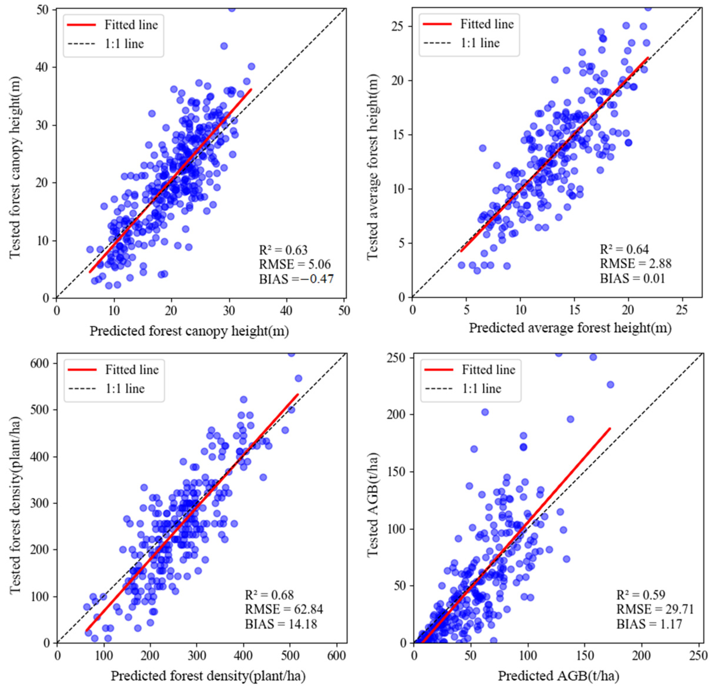
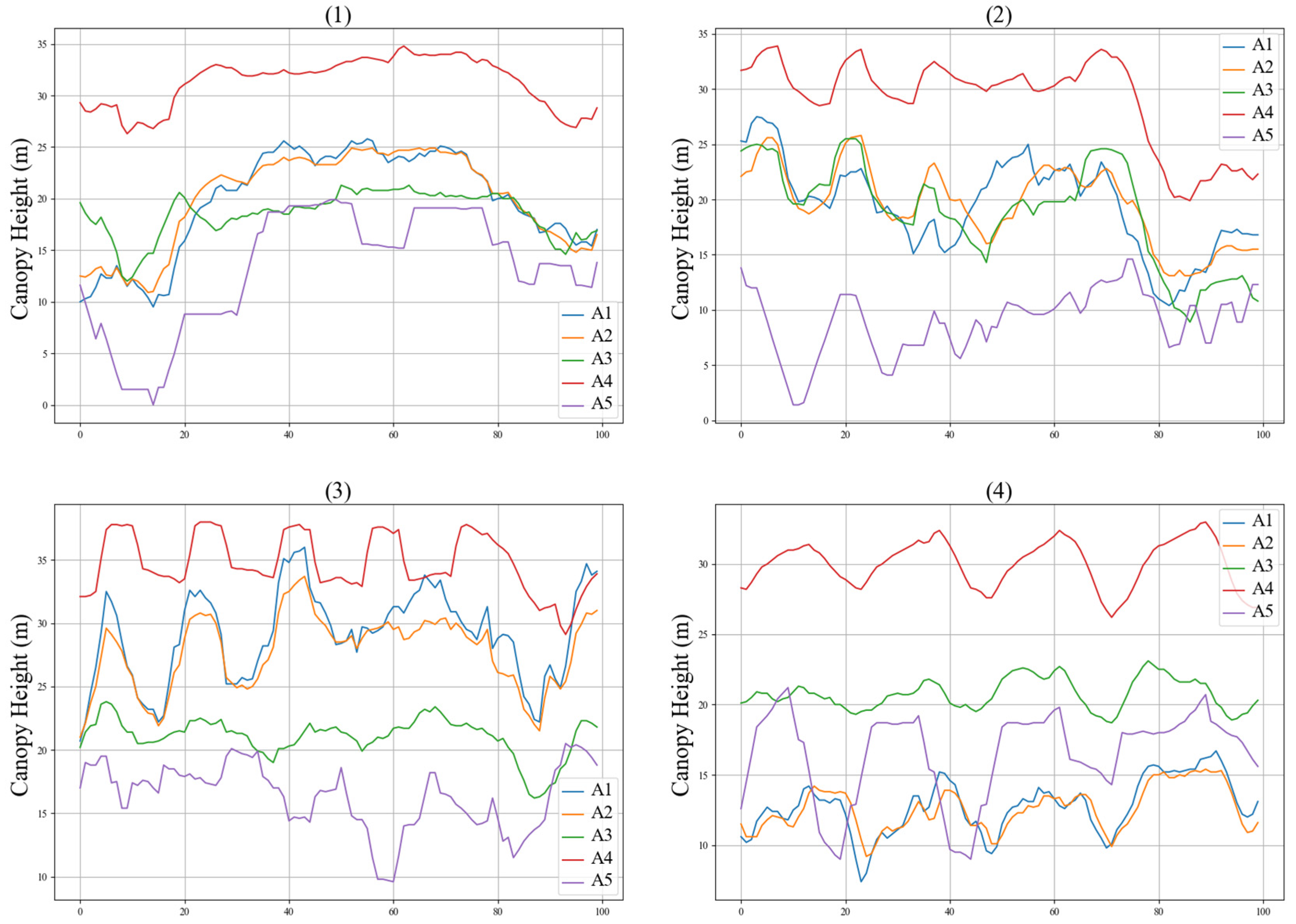
3.3. Accuracy Assessment of the Forest Structural Parameter Estimation

Estimation models were created for four forest structural parameters using selected variables. The aim was to assess the capabilities of SRTM DEM, Sentinel-1, and Aentinel-2 in forest structural parameter estimation. Using 20% of the sample data (N = 363), accuracy assessments were conducted. Figure 6 displays scatter plots of tested values versus estimated values, along with the corresponding linear regression lines.

Based on the data presented in Figure 6, the accuracy of the forest canopy height model was evaluated, which resulted in R² = 0.63, RMSE = 5.06, and BIAS = −0.47. The accuracy metrics for the forest average height model were R² = 0.64, RMSE = 2.88, and BIAS = 0.01. For the forest density model, the assessment resulted in R² = 0.68, RMSE = 62.84, and BIAS = 14.18. The forest AGB model demonstrated accuracy indicators of R² = 0.59, RMSE = 29.71, and BIAS = 1.17. Excellent simulation abilities were displayed by all the estimation models.

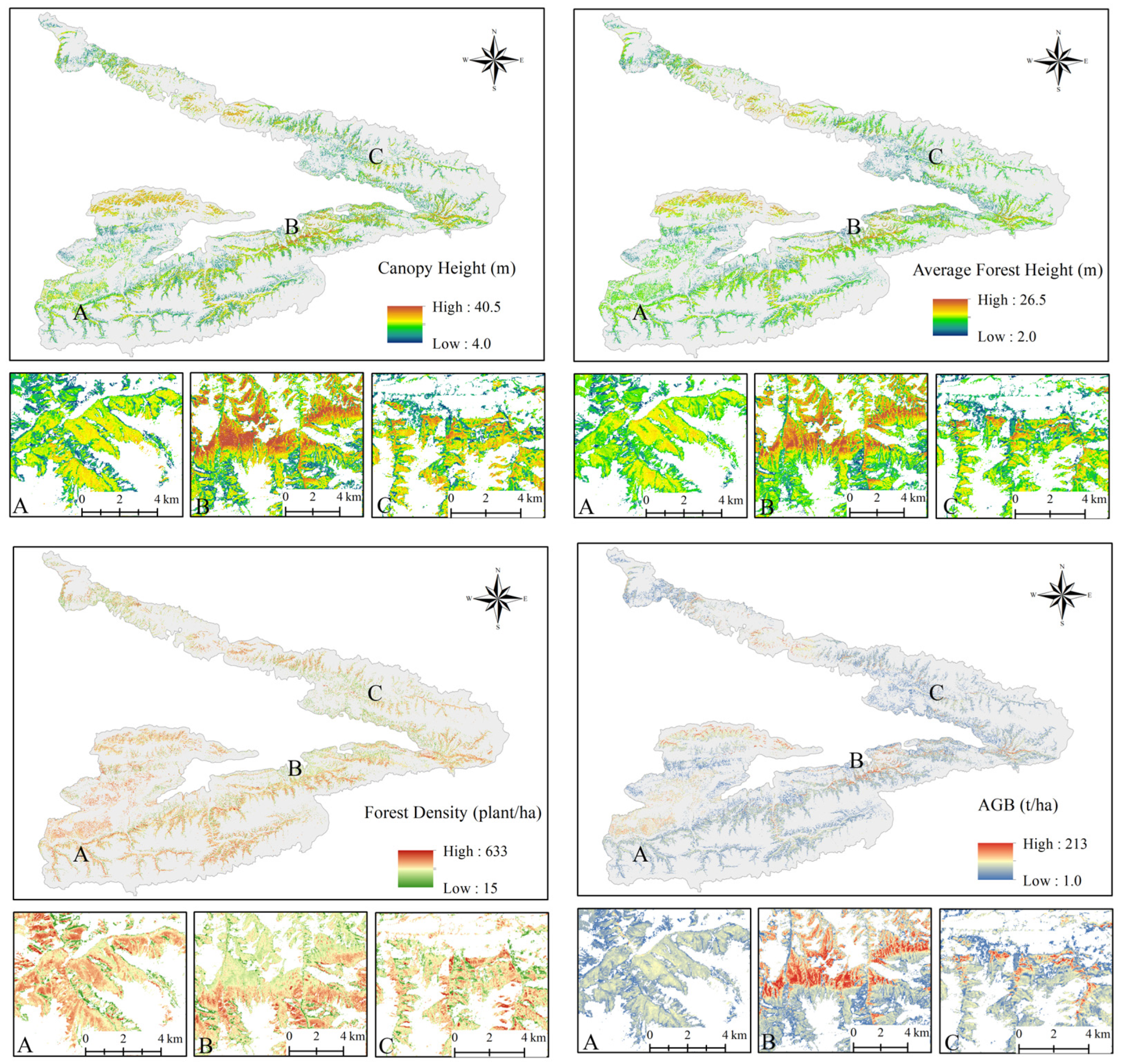
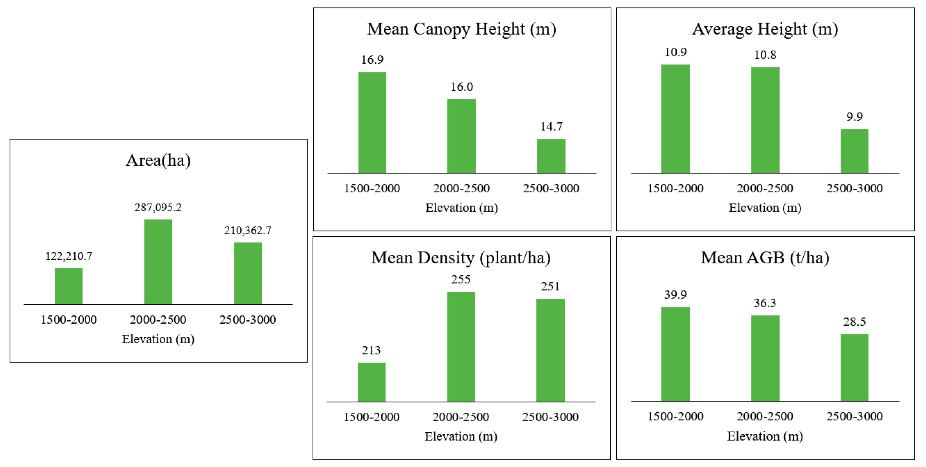
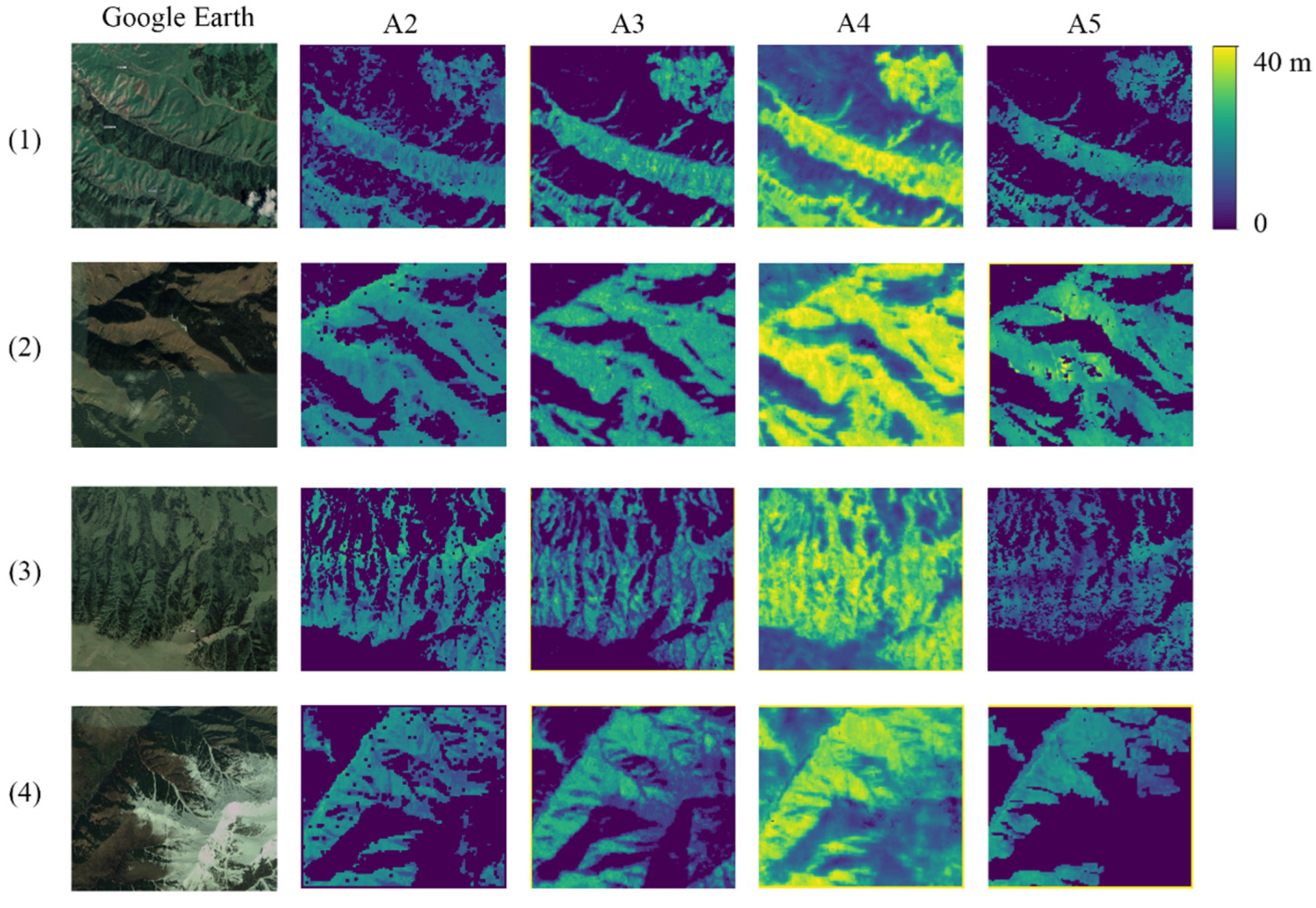
3.4. Results of the Forest Structural Parameters

Four estimation models based on the Bayesian-Random Forest regression model were used to estimate the results for the study area. The input data for the models were STRM DEM, Sentinel-1, and Sentinel-2.

Figure 7 shows that taller trees are mainly distributed in the southern part of the study area. Based on the observation of the localized map and DEM, the taller trees are distributed at lower elevations in the same area. This phenomenon is strongly related to growth conditions such as water-heat combinations, soil fertility, and so on. Usually, Schrenk spruce grows well on the north slopes with adequate soil fertility, high humidity, warmth, and no direct sunlight in the Tianshan Mountains. As the elevation increases, the temperature gradually decreases, which also affects Schrenk spruce growth. Additionally, there was a significant positive correlation between forest AGB and tree height because AGB comes from a single tree’s height. Similarly, the taller the tree, the lower the density.

To analyze tree growth in different altitude ranges, the study area was divided into altitude intervals of 1500~2000 m, 2000~2500 m, and 2500~3000 m based on the digital elevation model (DEM). Forest structural parameters have been assessed at each of these distinct altitudes. Figure 8 shows the statistical findings. Forests are predominantly situated on the northern slopes at elevations between 2000 and 2500 m, which is also the area with the highest density of forests. With increasing elevation, there’s a noticeable decrease in both the height of the forest canopy and the average tree height, along with a reduction in the aboveground biomass per unit area.

4. Discussion

4.1. UAV-LiDAR Data for Measuring Forest Structure Parameters

This study used point cloud data from an L1 sensor mounted on a DJI M300 UAV for forest structural parameter interpretation. UAV-LiDAR data are well-suited for coniferous forest structure estimation at the plot level, offering high spatial resolution and detailed topographic insights [35]. LiDAR stands out as a superior method for measuring direct canopy height [36]. The top-down data acquisition method is consistent with satellite data, facilitating enhanced spatial integration [13,16]. UAV-LiDAR minimizes ecosystem disruption while providing the flexibility of data acquisition through adaptable flight trajectories, optimizing data coverage, and sampling density for thorough forest structure characterization [37]. Visualizing LiDAR data as points and DEMs allows intuitive three-dimensional exploration of forest structure. Coupled with GIS and other tools, spatial analysis and modeling facilitate parameter extraction and detailed structural assessment [38]. Tianshan’s forest features, primarily spruce species, lend themselves to effective LiDAR use in capturing forest structure parameters. Their regular tree shapes, tower-like crowns, and limited bifurcations enable precise extraction using UAV-LiDAR data.

In complex and dense forests, UAV-LiDAR data can lead to reduced accuracy in tree parameter estimation. Challenges arise from understory trees being missed in the UAV-LiDAR point cloud and similar-looking canopies being wrongly identified as individual treetops. Conversely, local maxima not related to treetops can also be misinterpreted. Figure 9 demonstrates single-tree segmentation results for both spruce forests and mixed forests. Spruce forests (Figure 9a) with uniform canopies produce better segmentation outcomes due to minimal canopy intersections. On the other hand, the irregular and intersected canopies of mixed forests (Figure 9b) decrease segmentation accuracy. To address intricate forest parameters, complementing UAV-LiDAR with other data like terrestrial laser scanning (TLS) and mobile laser scanning (MLS) is necessary [39,40].

4.2. Relevance of Forest Structural Parameters with Predictive Variables

From the results on the importance of variables presented in Section 3.2, the most contributing variables have been identified and retained for each of the forest structural parameter estimation models (Figure 5).

DEM plays a crucial role in estimating forest structural parameters and exhibiting distinct correlations. Topographic factors intricately affect vegetation growth, stand structure, and species composition by modifying hydrothermal conditions [41]. Precipitation exhibits significant variations with changes in altitude. Rapid changes in elevation cause obstruction of air mass movement to form terrain rains and can also cause air mass to rise to form terrain rains. As the air mass loses water vapor, there will be less precipitation at higher altitudes, or the air mass will roll over the mountain and bring dryness to the leeward slopes. For every 100 m of elevation increase, the temperature will decrease by 0.6 °C. Differences in ground cover will also affect the temperature. Furthermore, varying slopes have an impact on soil layer depth and nutrient content. Steeper slopes tend to be less conducive to substantial soil layer development, and the nutrients in the soil are relatively shielded from rainfall compared to gentler slopes. These changes in climate and soil due to elevation, slope, and aspect directly affect the growth of the trees. Acknowledging the impact of topography on forest structure parameter estimation aligns with existing research [42,43], emphasizing the significance of topographical influence on forest attributes.

The backscattering data in VH and VV polarization offer substantial potential for estimating forest structural parameters. Sentinel-1 SAR C-band penetrates the upper canopies and interacts with foliage, making backscatter values indicative of forest structure [19]. VV-polarized and VH-polarized data exhibit distinct responses when interacting with vegetation and ground surfaces. This polarization discrepancy enables the inference of vegetation structure [14]. Various vegetation types show differing scattering traits under VV and VH polarizations. Dense vegetation like forests produces strong reflection signals in SAR images, while sparser vegetation like grasslands shows weaker signals.

Sentinel-2 is widely recognized for its pivotal role in vegetation monitoring. Specifically, the spectral bands B4, B5, B6, B7, B8, and B8A offer distinct advantages for evaluating various aspects of vegetation, including its coverage, health, leaf physiology, and photosynthetic efficiency. Integrating spectral data with forest structural parameters can significantly enhance the accuracy of the assessment. In previous studies, it has been observed that a significant correlation between the near-infrared (NIR) and short-wave infrared (SWIR) bands of Sentinel-2 and forest structural parameters persists regardless of environmental conditions. These correlations have proven to be a reliable means of achieving highly accurate results [13,15,44]. NDVI, computed from the near-infrared band (B8) and the red band (B4) of Sentinel-2, serves a wide range of applications, particularly in the assessment of surface vegetation cover and overall vegetation health [45,46]. It is also widely acknowledged as a fundamental vegetation index, extensively used in the modeling of forest structural parameters [13,14].

4.3. Comparison with Other Forest Canopy Height Products

To assess the model’s accuracy, LiDAR-measured forest canopy heights were compared with our estimated forest canopy heights and three other authors’ results [47,48,49]. These three studies used machine learning or deep learning methods to simulate forest canopy height, the reference data extracted by GEDI (Global Ecosystem Dynamics Investigation) data, and our study’s reference data extracted by UAV-LiDAR. We chose only the results of the canopy height simulation because it was difficult to find other forest structure parameters. The selected canopy height products are all current, dating from the post-2020 period.

Four sample plots were randomly selected among the estimates for comparison. To capture trend differences effectively, a sliding mean was applied to the five datasets, as presented in Figure 10. LiDAR-measured forest canopy height (A1) exhibited strong alignment with our model’s estimate (A2), which confirms the model’s high accuracy in representing Tianshan forest conditions. Other results also showed consistency with A1; however, A4 displayed overestimation, A5 underestimated, and A3 matched measured values in some plots but lacked precision compared to our model’s estimates. The selected studies have advantages in describing large-scale forests and have important implications for understanding the current state of global forests. Our model has higher accuracy, and this accuracy will better serve forest management.

Upon visual inspection of the comparison presented in Figure 11, it becomes evident that A2 and A5 exhibit distinct accuracy in delineating the forest boundary. Despite being able to identify the forest boundary, A3 encounters challenges in identifying small clearings inside the forest. On the other hand, the A4 model not only struggles to accurately identify the forest boundary but also demonstrates a noticeable tendency to overestimate forest canopy height.

Our model performed well in both accurate height estimation and precise forest boundary extraction. The datasets obtained by others also exhibit a high level of accuracy, particularly when characterizing the current state of large-scale forests. The superior performance of our estimated results is attributed to the accuracy, quantity, and representativeness of the training data, which is difficult to achieve with global models [50]. It is worth noting that trees of the same height but different species exhibit variations in spectral reflectance values. Even for the same tree species, a very limited number of samples cannot accurately depict the general characteristics of this species. Consequently, the quantity and representativeness of the samples used in modeling forest canopy height significantly influence the model’s estimation results. Using a large number of samples, a substantial enhancement in the accuracy of our training model created for single-species forests was achieved. This improvement holds substantial significance for the focused exploration of specific forest types.

5. Conclusions

In this study, forest canopy height, average height, density, and AGB for natural Schrenk spruce forests in the western Tianshan Mountains were successfully estimated. We used a machine learning model called Bayesian-Random Forest, using data from UVA-LiDAR to measure the forest structural parameters and data from STRM DEM, Sentinel 1, and Sentinel 2 to predict these parameters. This is the first time such extensive UAV-LiDAR data have been used to estimate forest characteristics in this region. The Bayesian optimizer efficiently found the best parameters for the Random Forest model and created accurate predictions in a short time. Based on the prediction results, the largest forest area, the highest forest height, the highest density, and the larger AGB were distributed in the 2000–2500 altitude range of the western Tianshan Mountains. Additionally, all forest structural parameters exhibit a gradual decrease with increasing mountain altitude. This is crucial knowledge for researching how climate change affects forests in Central Asia and is useful for comprehending the growth and ecological function of Schrenk spruce forests.

References

- Chen, B.; Wang, X. The importance, exploitation and utilization of China’s forest in arid mountainous regions. Temp. For. Ecosyst. 1986, 78, 78–79. [Google Scholar]
- Venäläinen, A.; Lehtonen, I.; Laapas, M.; Ruosteenoja, K.; Tikkanen, O.; Viiri, H.; Ikonen, V.; Peltola, H. Climate change induces multiple risks to boreal forests and forestry in Finland: A literature review. Glob. Chang. Biol. 2020, 26, 4178–4196. [Google Scholar] [CrossRef] [PubMed]
- Brodribb, T.J.; Powers, J.; Cochard, H.; Choat, B. Hanging by a thread? Forests and drought. Science 2020, 368, 261–266. [Google Scholar] [CrossRef] [PubMed]
- Feng, G.; Zhang, J.; Girardello, M.; Pellissier, V.; Svenning, J. Forest canopy height co-determines taxonomic and functional richness, but not functional dispersion of mammals and birds globally. Glob. Ecol. Biogeogr. 2020, 29, 1350–1359. [Google Scholar] [CrossRef]
- Hui, G.; Zhang, G.; Zhao, Z.; Yang, A. Methods of Forest Structure Research: A Review. Curr. For. Rep. 2019, 5, 142–154. [Google Scholar] [CrossRef]
- Roll, U.; Geffen, E.; Yom-Tov, Y. Linking vertebrate species richness to tree canopy height on a global scale. Glob. Ecol. Biogeogr. 2015, 24, 814–825. [Google Scholar] [CrossRef]
- Batista, G.E.A.P.A.; Prati, R.C.; Monard, M.C. A study of the behavior of several methods for balancing machine learning training data. ACM SIGKDD Explor. Newsl. 2004, 6, 20–29. [Google Scholar] [CrossRef]
- Batta, M. Machine Learning Algorithms—A Review. Int. J. Sci. Res. 2018, 18, 381–386. [Google Scholar] [CrossRef]
- Lv, J.; Wang, Z.; Yang, Y.; Qu, Y. Height Extraction and Growing Stock Inversion of Picea schrenkiana var. tianshanica in Tianshan Mountain Based on UAV Image. Xinjiang Agric. Sci. 2021, 58, 1838–1845. [Google Scholar]
- Su, Y.; Guo, Q.; Jin, S.; Guan, H.; Sun, X.; Ma, Q.; Hu, T.; Wang, R.; Li, Y. The Development and Evaluation of a Backpack LiDAR System for Accurate and Efficient Forest Inventory. IEEE Geosci. Remote Sens. Lett. 2020, 18, 1660–1664. [Google Scholar] [CrossRef]
- Cao, L.; Liu, K.; Shen, X.; Wu, X.; Liu, H. Estimation of Forest Structural Parameters Using UAV-LiDAR Data and a Process-Based Model in Ginkgo Planted Forests. IEEE J. Sel. Top. Appl. Earth Obs. Remote Sens. 2019, 12, 4175–4190. [Google Scholar] [CrossRef]
- Atkins, J.W.; Bohrer, G.; Fahey, R.T.; Hardiman, B.S.; Morin, T.H.; Stovall, A.E.L.; Zimmerman, N.; Gough, C.M. Quantifying vegetation and canopy structural complexity from terrestrial LiDAR data using the forestr r package. Methods Ecol. Evol. 2018, 9, 2057–2066. [Google Scholar] [CrossRef]
- Wang, D.; Wan, B.; Liu, J.; Su, Y.; Guo, Q.; Qiu, P.; Wu, X. Estimating aboveground biomass of the mangrove forests on northeast Hainan Island in China using an upscaling method from field plots, UAV-LiDAR data and Sentinel-2 imagery. Int. J. Appl. Earth Obs. Geoinf. 2020, 85, 101986. [Google Scholar] [CrossRef]
- Castillo, J.A.A.; Apan, A.A.; Maraseni, T.N.; Salmo, S.G., III. Estimation and mapping of above-ground biomass of mangrove forests and their replacement land uses in the Philippines using Sentinel imagery. ISPRS J. Photogramm. Remote Sens. 2017, 134, 70–85. [Google Scholar] [CrossRef]
- Liu, Y.; Gong, W.; Xing, Y.; Hu, X.; Gong, J. Estimation of the forest stand mean height and aboveground biomass in Northeast China using SAR Sentinel-1B, multispectral Sentinel-2A, and DEM imagery. ISPRS J. Photogramm. Remote Sens. 2019, 151, 277–289. [Google Scholar] [CrossRef]
- Li, W.; Niu, Z.; Shang, R.; Qin, Y.; Wang, L.; Chen, H. High-resolution mapping of forest canopy height using machine learning by coupling ICESat-2 LiDAR with Sentinel-1, Sentinel-2 and Landsat-8 data. Int. J. Appl. Earth Obs. Geoinf. 2020, 92, 102163. [Google Scholar] [CrossRef]
- Kattenborn, T.; Lopatin, J.; Förster, M.; Braun, A.C.; Fassnacht, F.E. UAV data as alternative to field sampling to map woody invasive species based on combined Sentinel-1 and Sentinel-2 data. Remote Sens. Environ. 2019, 227, 61–73. [Google Scholar] [CrossRef]
- Pourshamsi, M.; Xia, J.; Yokoya, N.; Garcia, M.; Lavalle, M.; Pottier, E.; Balzter, H. Tropical forest canopy height estimation from combined polarimetric SAR and LiDAR using machine-learning. ISPRS J. Photogramm. Remote Sens. 2020, 172, 79–94. [Google Scholar] [CrossRef]
- Bauer-Marschallinger, B.; Cao, S.; Navacchi, C.; Freeman, V.; Reuß, F.; Geudtner, D.; Rommen, B.; Vega, F.C.; Snoeij, P.; Attema, E.; et al. The normalised Sentinel-1 Global Backscatter Model, mapping Earth’s land surface with C-band microwaves. Sci. Data 2021, 8, 277. [Google Scholar] [CrossRef]
- Corte, A.P.D.; Souza, D.V.; Rex, F.E.; Sanquetta, C.R.; Mohan, M.; Silva, C.A.; Zambrano, A.M.A.; Prata, G.; de Almeida, D.R.A.; Trautenmüller, J.W.; et al. Forest inventory with high-density UAV-Lidar: Machine learning approaches for predicting individual tree attributes. Comput. Electron. Agric. 2020, 179, 105815. [Google Scholar] [CrossRef]
- Liu, Y.; Wang, Y.; Zhang, J. New Machine Learning Algorithm: Random Forest. In Information Computing and Applications; Springer: Berlin/Heidelberg, Germany, 2012; Volume 7473, pp. 246–252. [Google Scholar] [CrossRef]
- Segal, M.R. Machine Learning Benchmarks and Random Forest Regression Publication Date Machine Learning Benchmarks and Random Forest Regression; Center for Bioinformatics and Molecular Biostatistics: San Francisco, CA, USA, 2004; p. 15. [Google Scholar]
- Rodriguez-Galiano, V.; Sanchez-Castillo, M.; Chica-Olmo, M.; Chica-Rivas, M.J.O.G.R. Machine learning predictive models for mineral prospectivity: An evaluation of neural networks, random forest, regression trees and support vector machines. Ore Geol. Rev. 2015, 71, 804–818. [Google Scholar] [CrossRef]
- Zhao, H.; Yao, J.; Li, X.; Tao, H. The characteristics of climate change in Xinjiang during 1961–2015. Acta Sci. Nat. Univ. Sunyatseni 2020, 59, 126–133. [Google Scholar]
- Su, H.; Sang, W.; Wang, Y.; Ma, K. Simulating Picea schrenkiana forest productivity under climatic changes and atmospheric CO2 increase in Tianshan Mountains, Xinjiang Autonomous Region, China. For. Ecol. Manag. 2007, 246, 273–284. [Google Scholar] [CrossRef]
- Lan, J.; Xiao, Z.; Li, J.; Zhang, Y. Biomass allocation and allometric growth of Picea schrenkiana in Tianshan Mountains. J. Zhejiang AF Univ. 2020, 37, 416–423. [Google Scholar]
- Breiman, L. Random Forests. Mach. Learn. 2001, 45, 5–32. [Google Scholar] [CrossRef]
- Wang, H.; Yilihamu, Q.; Yuan, M.; Bai, H.; Xu, H.; Wu, J. Prediction models of soil heavy metal(loid)s concentration for agricultural land in Dongli: A comparison of regression and random forest. Ecol. Indic. 2020, 119, 106801. [Google Scholar] [CrossRef]
- Ali, M.; Prasad, R.; Xiang, Y.; Yaseen, Z.M. Complete ensemble empirical mode decomposition hybridized with random forest and kernel ridge regression model for monthly rainfall forecasts. J. Hydrol. 2020, 584, 124647. [Google Scholar] [CrossRef]
- Sun, D.; Xu, J.; Wen, H.; Wang, D. Assessment of landslide susceptibility mapping based on Bayesian hyperparameter op-timization: A comparison between logistic regression and random forest. Eng. Geol. 2021, 281, 105972. [Google Scholar] [CrossRef]
- Zhang, W.; Wu, C.; Zhong, H.; Li, Y.; Wang, L. Prediction of undrained shear strength using extreme gradient boosting and random forest based on Bayesian optimization. Geosci. Front. 2020, 12, 469–477. [Google Scholar] [CrossRef]
- Snoek, J.; Larochelle, H.; Adams, R.P. Practical Bayesian Optimization of Machine Learning Algorithms. Adv. Neural Inf. Process. Syst. 2012, 25, 2960–2968. [Google Scholar] [CrossRef]
- Martinez-Cantin, R. BayesOpt: A Bayesian optimization library for nonlinear optimization, experimental design and bandits. J. Mach. Learn. Res. 2015, 15, 3735–3739. [Google Scholar]
- Fabian, P.; Gael, V.; Alexandre, G.; Vincent, M.; Bertrand, T. Scikit-learn: Machine Learning in Python Fabian. J. Mach. Learn. Res. 2011, 12, 2825–2830. [Google Scholar] [CrossRef]
- Qiu, Q.; Zhang, W.; Wang, L.; Cao, S.; Sun, W. Estimation of Single Wood Factor of Picea schrenkiana var. tianshanica Forest Based on Backpack LiDAR. For. Resour. Manag. 2021, 4, 99. [Google Scholar]
- Wang, Y.; Lehtomäki, M.; Liang, X.; Pyörälä, J.; Kukko, A.; Jaakkola, A.; Liu, J.; Feng, Z.; Chen, R.; Hyyppä, J. Is field-measured tree height as reliable as believed—A comparison study of tree height estimates from field measurement, airborne laser scanning and terrestrial laser scanning in a boreal forest. ISPRS J. Photogramm. Remote Sens. 2018, 147, 132–145. [Google Scholar] [CrossRef]
- Puliti, S.; Ene, L.T.; Gobakken, T.; Næsset, E. Use of partial-coverage UAV data in sampling for large scale forest inventories. Remote Sens. Environ. 2017, 194, 115–126. [Google Scholar] [CrossRef]
- Liu, K.; Shen, X.; Cao, L.; Wang, G.; Cao, F. Estimating forest structural attributes using UAV-LiDAR data in Ginkgo plantations. ISPRS J. Photogramm. Remote Sens. 2018, 146, 465–482. [Google Scholar] [CrossRef]
- Dai, W.; Yang, B.; Dong, Z.; Shaker, A. A new method for 3D individual tree extraction using multispectral airborne LiDAR point clouds. ISPRS J. Photogramm. Remote Sens. 2018, 144, 400–411. [Google Scholar] [CrossRef]
- Yang, B.; Dai, W.; Dong, Z.; Liu, Y. Automatic Forest Mapping at Individual Tree Levels from Terrestrial Laser Scanning Point Clouds with a Hierarchical Minimum Cut Method. Remote Sens. 2016, 8, 372. [Google Scholar] [CrossRef]
- Crimmins, T.M.; Crimmins, M.A.; Bertelsen, C.D. Complex responses to climate drivers in onset of spring flowering across a semi-arid elevation gradient. J. Ecol. 2010, 98, 1042–1051. [Google Scholar] [CrossRef]
- Saatchi, S.; Marlier, M.; Chazdon, R.L.; Clark, D.B.; Russell, A.E. Impact of spatial variability of tropical forest structure on radar estimation of aboveground biomass. Remote Sens. Environ. 2011, 115, 2836–2849. [Google Scholar] [CrossRef]
- Ediriweera, S.; Danaher, T.; Pathirana, S. The influence of topographic variation on forest structure in two woody plant communities: A remote sensing approach. For. Syst. 2016, 25, e049. [Google Scholar] [CrossRef]
- Nandy, S.; Srinet, R.; Padalia, H. Mapping Forest Height and Aboveground Biomass by Integrating ICESat-2, Sentinel-1 and Sentinel-2 Data Using Random Forest Algorithm in Northwest Himalayan Foothills of India. Geophys. Res. Lett. 2021, 48, e2021GL093799. [Google Scholar] [CrossRef]
- Spruce, J.P.; Sader, S.; Ryan, R.E.; Smoot, J.; Kuper, P.; Ross, K.; Prados, D.; Russell, J.; Gasser, G.; McKellip, R.; et al. Assessment of MODIS NDVI time series data products for detecting forest defoliation by gypsy moth outbreaks. Remote Sens. Environ. 2011, 115, 427–437. [Google Scholar] [CrossRef]
- Dash, J.P.; Watt, M.S.; Pearse, G.D.; Heaphy, M.; Dungey, H.S. Assessing very high resolution UAV imagery for monitoring forest health during a simulated disease outbreak. ISPRS J. Photogramm. Remote Sens. 2017, 131, 1–14. [Google Scholar] [CrossRef]
- Liu, X.; Su, Y.; Hu, T.; Yang, Q.; Liu, B.; Deng, Y.; Tang, H.; Tang, Z.; Fang, J.; Guo, Q. Neural network guided interpolation for mapping canopy height of China’s forests by integrating GEDI and ICESat-2 data. Remote Sens. Environ. 2022, 269, 112844. [Google Scholar] [CrossRef]
- Lang, N.; Jetz, W.; Schindler, K.; Wegner, J.D. A High-Resolution Canopy Height Model of the Earth. 2022. Available online: http://arxiv.org/abs/2204.08322 (accessed on 1 July 2023).
- Potapov, P.; Li, X.; Hernandez-Serna, A.; Tyukavina, A.; Hansen, M.C.; Kommareddy, A.; Pickens, A.; Turubanova, S.; Tang, H.; Silva, C.E.; et al. Mapping global forest canopy height through integration of GEDI and Landsat data. Remote Sens. Environ. 2020, 253, 112165. [Google Scholar] [CrossRef]
- Moghaddam, D.D.; Rahmati, O.; Panahi, M.; Tiefenbacher, J.; Darabi, H.; Haghizadeh, A.; Haghighi, A.T.; Nalivan, O.A.; Tien Bui, D. The effect of sample size on different machine learning models for groundwater potential mapping in mountain bedrock aquifers. CATENA 2020, 187, 104421. [Google Scholar] [CrossRef]