
MFINet: Multi-Scale Feature Interaction Network for Change Detection of High-Resolution Remote Sensing Images


Abstract
:1. Introduction
- 1.
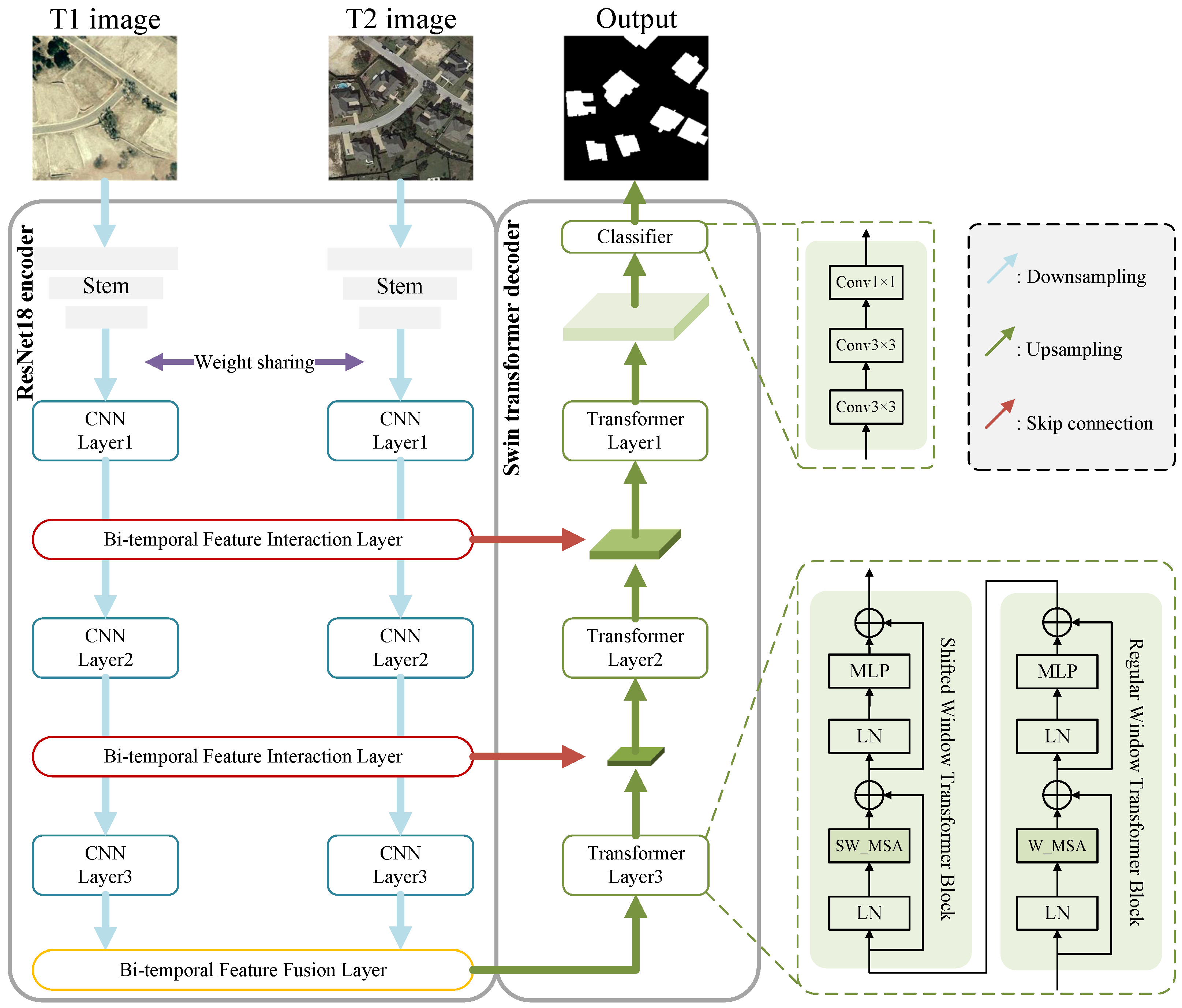
- A remote sensing image change detection network based on a multi-scale feature interaction structure named MFINet is proposed to solve the problem of insufficient target attention caused by insufficient bi-temporal interaction in change detection tasks. In the overall structure, we use a combination of a CNN encoder and a transformer decoder to make full use of the CNN’s local perception and the transformer’s global receptive field to effectively understand different levels of multi-source information.
- 2.
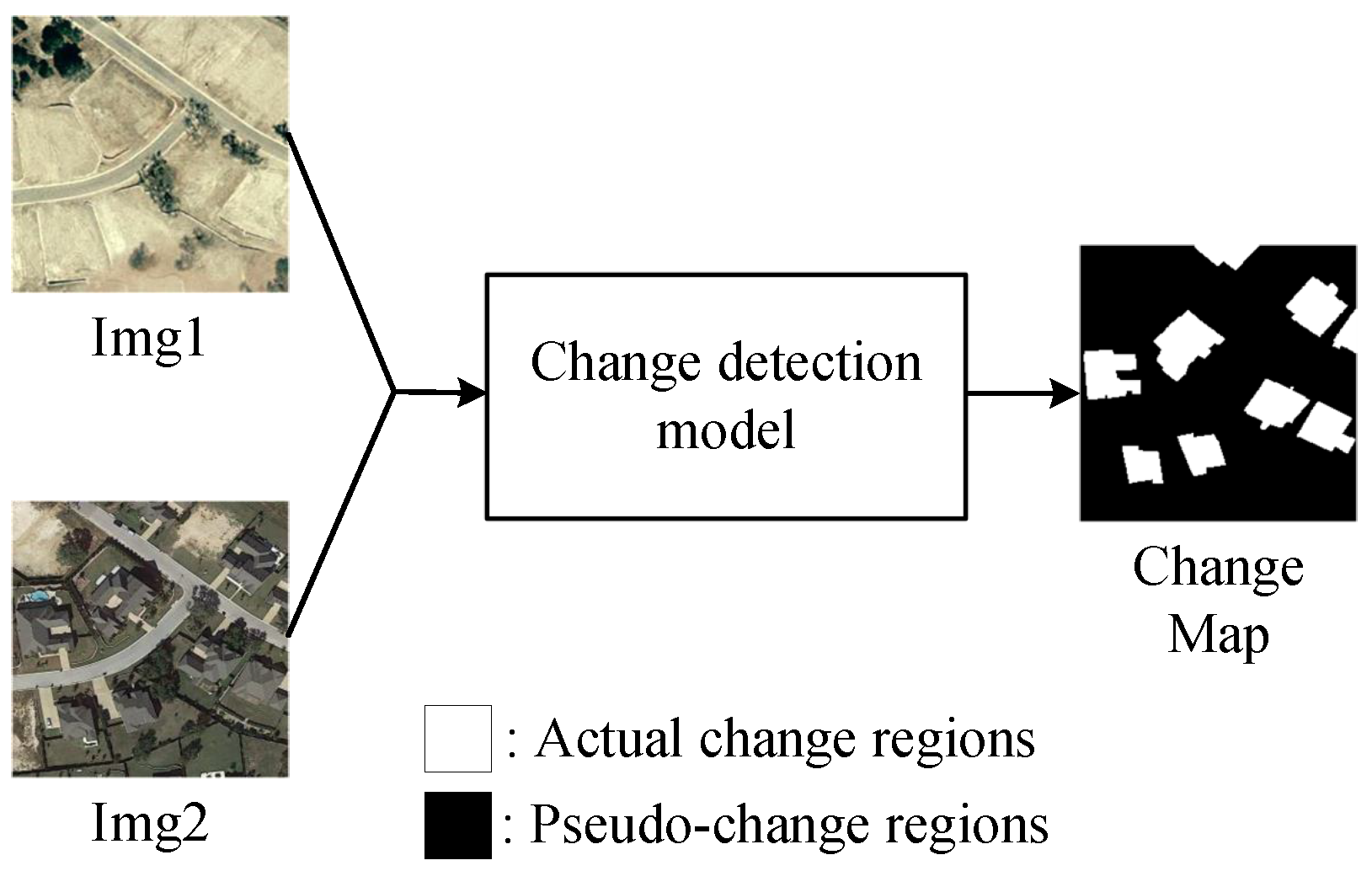
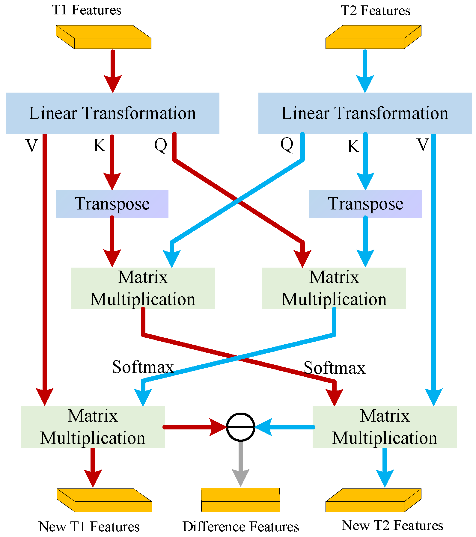
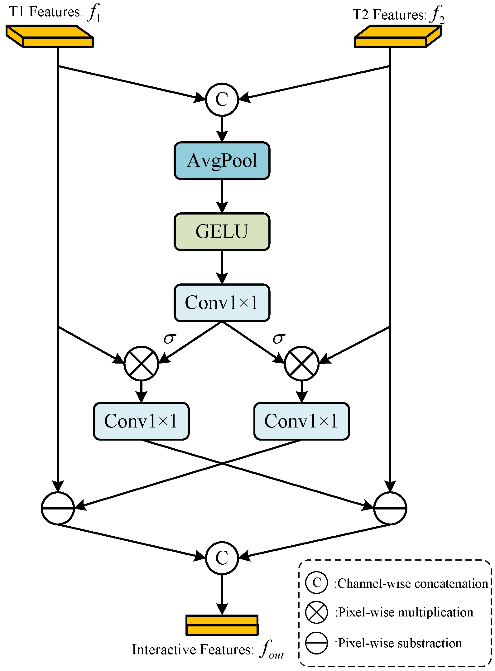
- A bi-temporal feature interaction layer (BFIL) is proposed to act as a medium for multi-level feature interaction, enhance the semantic information exchange between the same-level features of the Siamese network, and enhance the multi-temporal information communication at different time nodes. It is conducive to the model to discover the actual change regions and suppress the interference of the pseudo-change region.
- 3.
- In order to strengthen the model’s perception of the fine-grained difference between the bi-temporal deep processing features, we propose the bi-temporal feature fusion layer (BFFL), which integrates rich bi-temporal deep features before image size restoration by constructing bi-temporal homologous global guidance features.
2. Related Work
2.1. CNN-Based Change Detection Methods
2.2. Transformer-Based Change Detection Methods
3. Methodology
3.1. Overall Structure
3.2. Bi-Temporal Feature Interaction Layer
3.3. Bi-Temporal Feature Fusion Layer
3.4. Multi-Scale Decoding Layer Based on Transformer
4. Experiment
4.1. Datasets
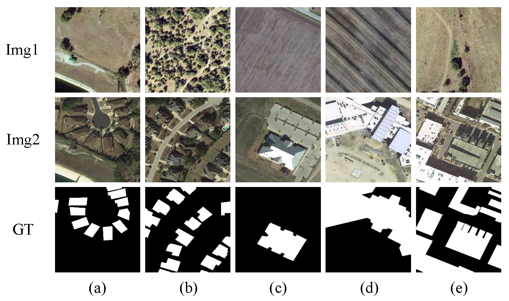
4.1.1. LEVIR-CD
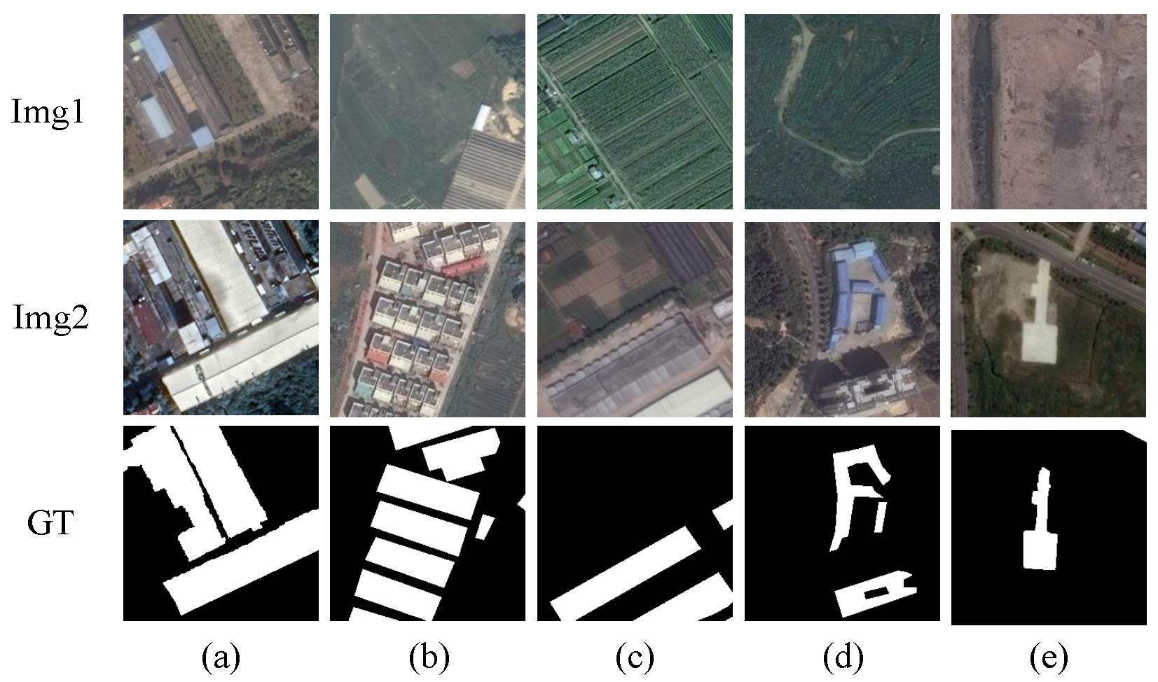
4.1.2. GZ-CD
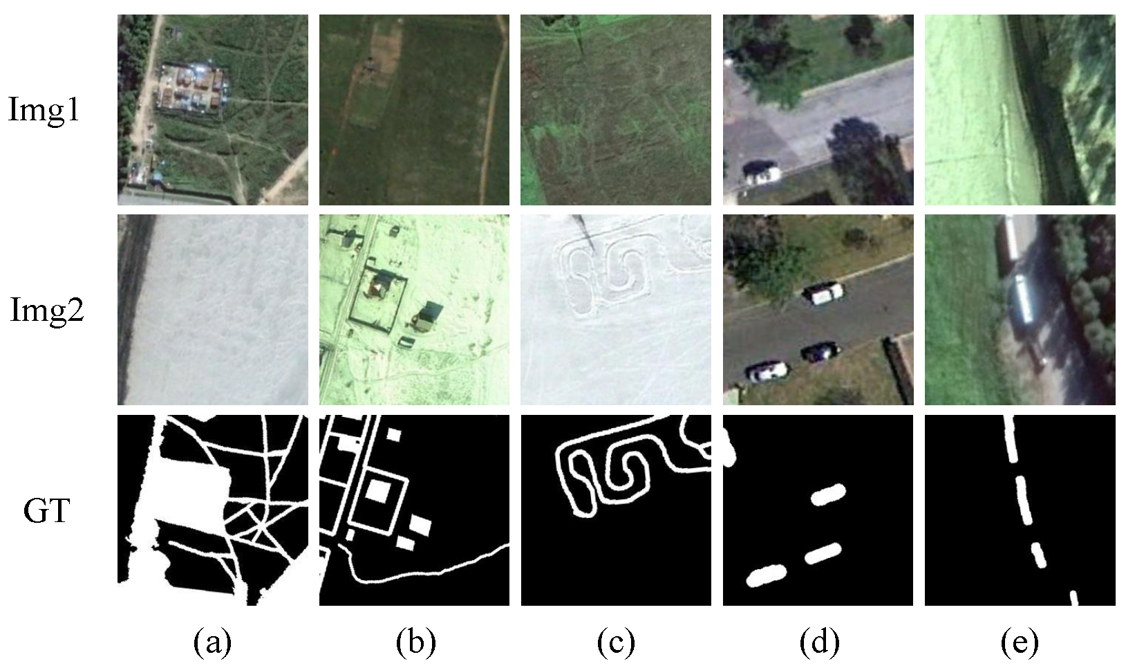
4.1.3. Lebedev Dataset
4.2. Implementation Details
4.3. Ablation Experiments on LEVIR-CD
- 1.
- The influence of BFIL: It is difficult for a simple twin CNN network to discover the common and different features of bi-temporal features, and the ability of bi-temporal mutual understanding will become worse as the number of layers deepens. Therefore, we added a BFIL to the backbone network to strengthen the interactive attributes of bi-temporal features, and used the attention weight as an interactive means. The experimental results show that the BFIL can help the network to improve the accurate detection of changing targets in the coding stage. For LEVIR-CD, F1 increased by 0.99% and IoU increased by 2.54%. For GZ-CD, F1 increased by 1.39% and IoU increased by 2.52%.
- 2.
- The influence of BFFL: The fusion operation of deep bi-temporal features is a great test of the lightweight degree and differential feature extraction ability of the module. It is easy to confuse features using simple pixel subtraction or channel cascade, while BFFL reduces the occurrence of feature confusion through multiple residual connections. The experimental results show that the BFFL bi-temporal feature fusion significantly increases the segmentation accuracy of the changed region features. For LEVIR-CD, F1 increased by 0.58% and IoU increased by 0.98%. For GZ-CD, F1 increased by 0.81% and IoU increased by 0.22%.
- 3.
- The influence of decoder selection: We compared two kinds of decoder methods. One is ResNet18, which is consistent with the encoder, and the other is the swin transformer used in our model. In terms of experimental results, the improvement in indicators in the changing region is limited. The F1 for LEVIR-CD increased by 0.16%, and IoU increased by 0.21%. For GZ-CD, F1 increased by 0.49% and IoU increased by 0.43%.
4.4. Comparative Experiments on Different Datasets
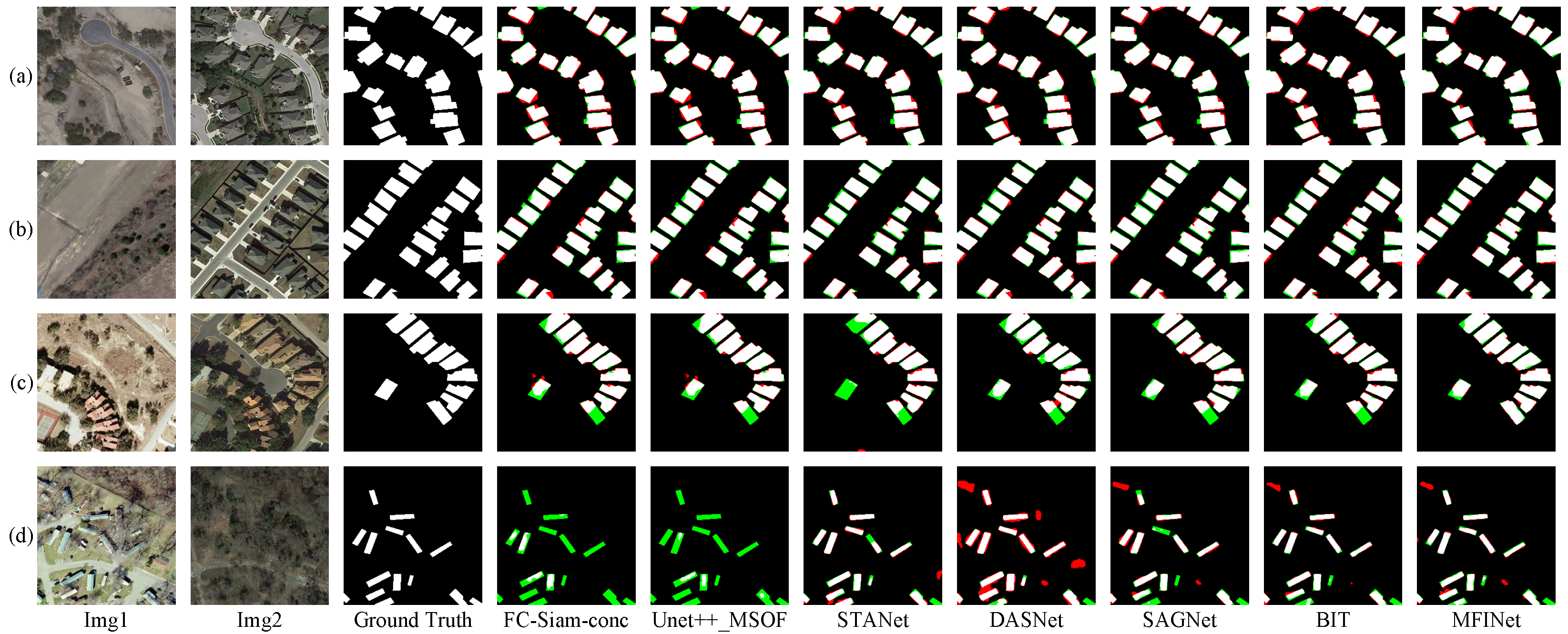
4.4.1. Comparative Experiments on LEVIR-CD
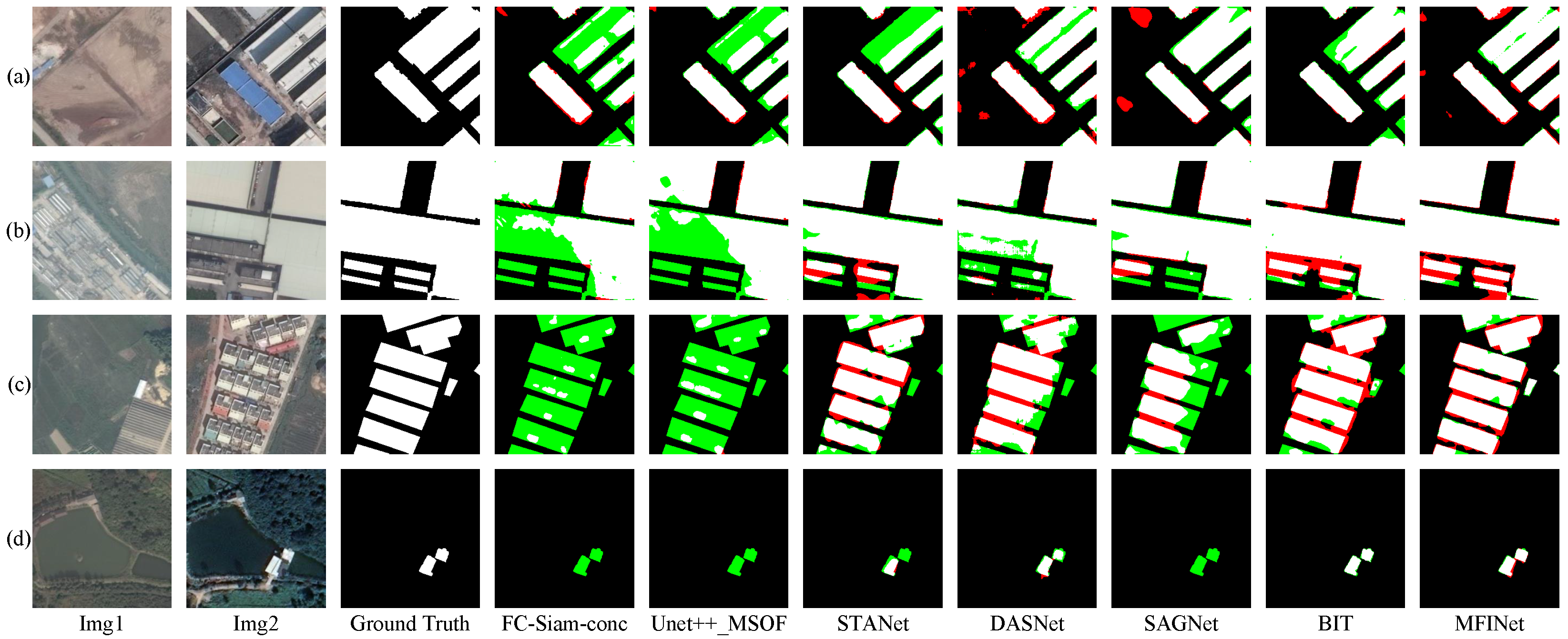
4.4.2. Comparative Experiments on GZ-CD
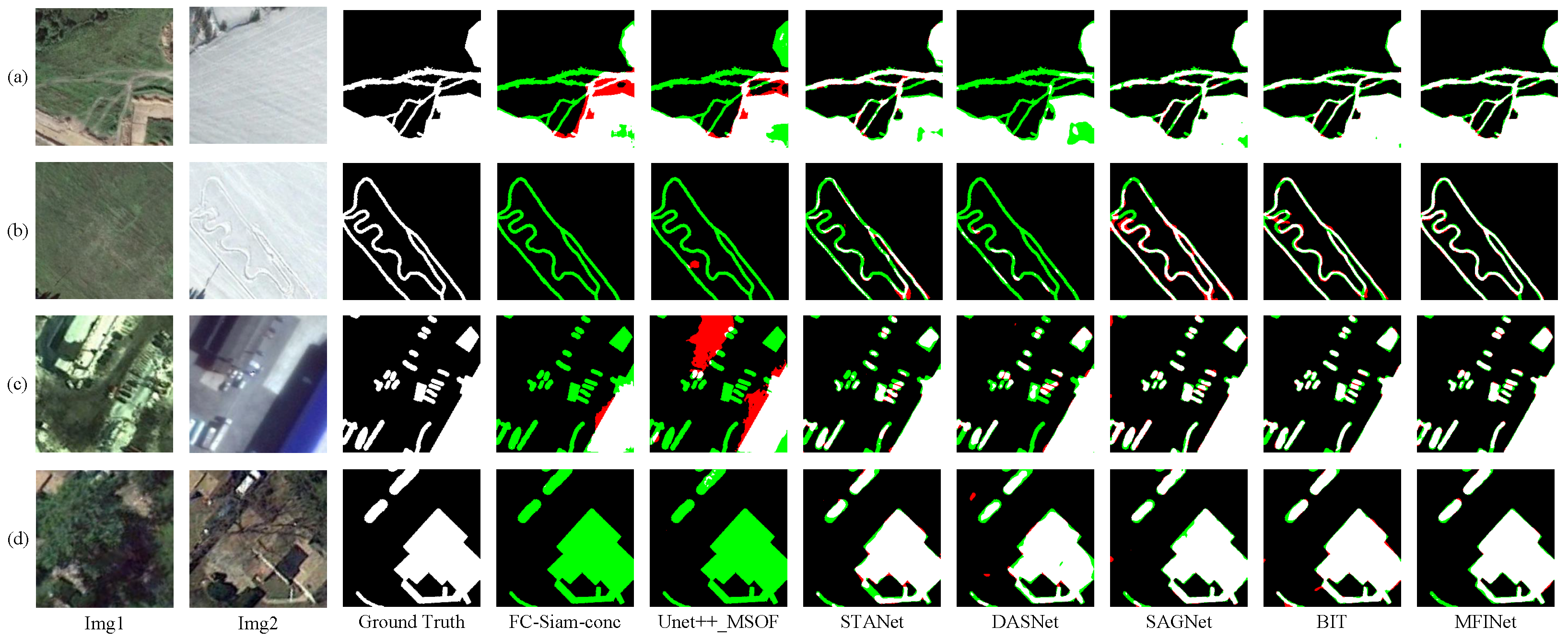
4.4.3. Comparative Experiments on Lebedev Dataset
4.5. Discussion
4.5.1. Comprehensive Efficiency Analysis of the Models
4.5.2. Model Characteristics and Future Prospects
5. Conclusions
Author Contributions
Funding
Data Availability Statement
Conflicts of Interest
References
- Ding, L.; Xia, M.; Lin, H.; Hu, K. Multi-Level Attention Interactive Network for Cloud and Snow Detection Segmentation. Remote Sens. 2024, 16, 112. [Google Scholar] [CrossRef]
- Peng, X.; Zhong, R.; Li, Z.; Li, Q. Optical Remote Sensing Image Change Detection Based on Attention Mechanism and Image Difference. IEEE Trans. Geosci. Remote Sns. 2021, 59, 7296–7307. [Google Scholar] [CrossRef]
- Marin, C.; Bovolo, F.; Bruzzone, L. Building Change Detection in Multitemporal Very High Resolution SAR Images. IEEE Trans. Geosci. Remote Sens. 2015, 53, 2664–2682. [Google Scholar] [CrossRef]
- Wang, Z.; Xia, M.; Weng, L.; Hu, K.; Lin, H. Dual Encoder–Decoder Network for Land Cover Segmentation of Remote Sensing Image. IEEE J. Sel. Top. Appl. Earth Obs. Remote Sens. 2024, 17, 2372–2385. [Google Scholar] [CrossRef]
- Fang, S.; Li, K.; Li, Z. Changer: Feature Interaction is What You Need for Change Detection. IEEE Trans. Geosci. Remote Sens. 2023, 61, 5610111. [Google Scholar] [CrossRef]
- Diakogiannis, F.; Waldner, F.; Caccetta, P. Looking for change? Roll the Dice and demand Attention. Remote Sens. 2021, 13, 3707. [Google Scholar] [CrossRef]
- Willis, K.S. Remote sensing change detection for ecological monitoring in United States protected areas. Biol. Conserv. 2015, 182, 233–242. [Google Scholar] [CrossRef]
- Jin, H.; He, W.; Liu, Q.; Wang, J.; Feng, G. The applicability of research on moving cut data-approximate entropy on abrupt climate change detection. Theor. Appl. Climatol. 2016, 124, 475–486. [Google Scholar] [CrossRef]
- Qiao, H.; Wan, X.; Wan, Y.; Li, S.; Zhang, W. A novel change detection method for natural disaster detection and segmentation from video sequence. Sensors 2020, 20, 5076. [Google Scholar] [CrossRef]
- Lunetta, R.S.; Knight, J.F.; Ediriwickrema, J.; Lyon, J.G.; Worthy, L.D. Land-cover change detection using multi-temporal MODIS NDVI data. In Geospatial Information Handbook for Water Resources and Watershed Management; CRC Press: Boca Raton, FL, USA, 2022; Volume II, pp. 65–88. [Google Scholar]
- Zhang, Z.; Liu, F.; Zhao, X.; Wang, X.; Shi, L.; Xu, J.; Yu, S.; Wen, Q.; Zuo, L.; Yi, L.; et al. Urban Expansion in China Based on Remote Sensing Technology: A Review. Chin. Geogr. Sci. 2018, 28, 727–743. [Google Scholar] [CrossRef]
- Rokni, K.; Ahmad, A.; Solaimani, K.; Hazini, S. A new approach for surface water change detection: Integration of pixel level image fusion and image classification techniques. Int. J. Appl. Earth Obs. Geoinf. 2015, 34, 226–234. [Google Scholar] [CrossRef]
- Wiratama, W.; Lee, J.; Sim, D. Change detection on multi-spectral images based on feature-level U-Net. IEEE Access 2020, 8, 12279–12289. [Google Scholar] [CrossRef]
- Xu, L.; Jing, W.; Song, H.; Chen, G. High-resolution remote sensing image change detection combined with pixel-level and object-level. IEEE Access 2019, 7, 78909–78918. [Google Scholar] [CrossRef]
- Maćkiewicz, A.; Ratajczak, W. Principal components analysis (PCA). Comput. Geosci. 1993, 19, 303–342. [Google Scholar] [CrossRef]
- Celik, T. Unsupervised Change Detection in Satellite Images Using Principal Component Analysis and k-Means Clustering. IEEE Geosci. Remote Sens. Lett. 2009, 6, 772–776. [Google Scholar] [CrossRef]
- Liu, S.; Du, Q.; Tong, X.; Samat, A.; Bruzzone, L.; Bovolo, F. Multiscale Morphological Compressed Change Vector Analysis for Unsupervised Multiple Change Detection. IEEE J. Sel. Top. Appl. Earth Obs. Remote Sens. 2017, 10, 4124–4137. [Google Scholar] [CrossRef]
- Bovolo, F.; Bruzzone, L.; Marconcini, M. A novel approach to unsupervised change detection based on a semisupervised SVM and a similarity measure. IEEE Trans. Geosci. Remote Sens. 2008, 46, 2070–2082. [Google Scholar] [CrossRef]
- Im, J.; Jensen, J.R. A change detection model based on neighborhood correlation image analysis and decision tree classification. Remote Sens. Environ. 2005, 99, 326–340. [Google Scholar] [CrossRef]
- Volpi, M.; Tuia, D.; Bovolo, F.; Kanevski, M.; Bruzzone, L. Supervised change detection in VHR images using contextual information and support vector machines. Int. J. Appl. Earth Obs. Geoinf. 2013, 20, 77–85. [Google Scholar] [CrossRef]
- Wang, X.; Liu, S.; Du, P.; Liang, H.; Xia, J.; Li, Y. Object-Based Change Detection in Urban Areas from High Spatial Resolution Images Based on Multiple Features and Ensemble Learning. Remote Sens. 2018, 11, 276. [Google Scholar] [CrossRef]
- Tan, K.; Zhang, Y.; Wang, X.; Chen, Y. Object-Based Change Detection Using Multiple Classifiers and Multi-Scale Uncertainty Analysis. Remote Sens. 2019, 10, 359. [Google Scholar] [CrossRef]
- Rawat, W.; Wang, Z. Deep convolutional neural networks for image classification: A comprehensive review. Neural Comput. 2017, 29, 2352–2449. [Google Scholar] [CrossRef] [PubMed]
- Vaswani, A.; Shazeer, N.; Parmar, N.; Uszkoreit, J.; Jones, L.; Gomez, A.N.; Kaiser, Ł.; Polosukhin, I. Attention is all you need. Adv. Neural Inf. Process. Syst. 2017, 30. [Google Scholar]
- Liu, M.; Chai, Z.; Deng, H.; Liu, R. A CNN-transformer network with multiscale context aggregation for fine-grained cropland change detection. IEEE J. Sel. Top. Appl. Earth Obs. Remote Sens. 2022, 15, 4297–4306. [Google Scholar] [CrossRef]
- Ren, H.; Xia, M.; Weng, L.; Hu, K.; Lin, H. Dual-Attention-Guided Multiscale Feature Aggregation Network for Remote Sensing Image Change Detection. IEEE J. Sel. Top. Appl. Earth Obs. Remote Sens. 2024, 17, 4899–4916. [Google Scholar] [CrossRef]
- Bandara, W.G.C.; Patel, V.M. A Transformer-Based Siamese Network for Change Detection. In Proceedings of the IGARSS 2022–2022 IEEE International Geoscience and Remote Sensing Symposium, Kuala Lumpur, Malaysia, 17–22 July 2022. [Google Scholar] [CrossRef]
- Zhan, Y.; Fu, K.; Yan, M.; Sun, X.; Wang, H.; Qiu, X. Change Detection Based on Deep Siamese Convolutional Network for Optical Aerial Images. IEEE Geosci. Remote Sens. Lett. 2017, 14, 1845–1849. [Google Scholar] [CrossRef]
- Daudt, R.C.; Le Saux, B.; Boulch, A. Fully convolutional siamese networks for change detection. In Proceedings of the 2018 25th IEEE International Conference on Image Processing (ICIP), Athens, Greece, 7–10 October 2018; pp. 4063–4067. [Google Scholar]
- Peng, D.; Zhang, Y.; Guan, H. End-to-End Change Detection for High Resolution Satellite Images Using Improved UNet++. Remote Sens. 2019, 11, 1382. [Google Scholar] [CrossRef]
- Zhang, C.; Yue, P.; Tapete, D.; Jiang, L.; Shangguan, B.; Huang, L.; Liu, G. A deeply supervised image fusion network for change detection in high resolution bi-temporal remote sensing images. ISPRS J. Photogramm. Remote Sens. 2020, 166, 183–200. [Google Scholar] [CrossRef]
- Yin, H.; Weng, L.; Li, Y.; Xia, M.; Hu, K.; Lin, H.; Qian, M. Attention-guided siamese networks for change detection in high resolution remote sensing images. Int. J. Appl. Earth Obs. Geoinf. 2023, 117, 103206. [Google Scholar] [CrossRef]
- Chen, H.; Shi, Z. A Spatial-Temporal Attention-Based Method and a New Dataset for Remote Sensing Image Change Detection. Remote Sens. 2020, 12, 1662. [Google Scholar] [CrossRef]
- Zhang, C.; Wang, L.; Cheng, S.; Li, Y. SwinSUNet: Pure transformer network for remote sensing image change detection. IEEE Trans. Geosci. Remote Sens. 2022, 60, 1–13. [Google Scholar] [CrossRef]
- Chen, H.; Qi, Z.; Shi, Z. Remote Sensing Image Change Detection With Transformers. IEEE Trans. Geosci. Remote Sens. 2022, 60, 1–14. [Google Scholar] [CrossRef]
- Feng, Y.; Jiang, J.; Xu, H.; Zheng, J. Change detection on remote sensing images using dual-branch multilevel intertemporal network. IEEE Trans. Geosci. Remote Sens. 2023, 61, 1–15. [Google Scholar] [CrossRef]
- Chen, C.P.; Hsieh, J.W.; Chen, P.Y.; Hsieh, Y.K.; Wang, B.S. SARAS-net: Scale and relation aware siamese network for change detection. In Proceedings of the AAAI Conference on Artificial Intelligence, Washington, DC, USA, 7–14 February 2023; Volume 37, pp. 14187–14195. [Google Scholar]
- Hendrycks, D.; Gimpel, K. A baseline for detecting misclassified and out-of-distribution examples in neural networks. arXiv 2016, arXiv:1610.02136. [Google Scholar]
- Yu, C.; Gao, C.; Wang, J.; Yu, G.; Shen, C.; Sang, N. Bisenet v2: Bilateral network with guided aggregation for real-time semantic segmentation. Int. J. Comput. Vis. 2021, 129, 3051–3068. [Google Scholar] [CrossRef]
- Peng, D.; Bruzzone, L.; Zhang, Y.; Guan, H.; Ding, H.; Huang, X. SemiCDNet: A Semisupervised Convolutional Neural Network for Change Detection in High Resolution Remote-Sensing Images. IEEE Trans. Geosci. Remote Sens. 2021, 59, 5891–5906. [Google Scholar] [CrossRef]
- Lebedev, M.A.; Vizilter, Y.V.; Vygolov, O.V.; Knyaz, V.A.; Rubis, A.Y. Change detection in remote sensing images using conditional adversarial networks. Int. Arch. Photogramm. Remote Sens. Spat. Inf. Sci. 2018, XLII-2, 565–571. [Google Scholar] [CrossRef]
- Fang, S.; Li, K.; Shao, J.; Li, Z. SNUNet-CD: A Densely Connected Siamese Network for Change Detection of VHR Images. IEEE Geosci. Remote Sens. Lett. 2022, 19, 1–5. [Google Scholar] [CrossRef]
- Yin, H.; Ma, C.; Weng, L.; Xia, M.; Lin, H. Bitemporal Remote Sensing Image Change Detection Network Based on Siamese-Attention Feedback Architecture. Remote Sens. 2023, 15, 4186. [Google Scholar] [CrossRef]
- Chen, J.; Yuan, Z.; Peng, J.; Chen, L.; Huang, H.; Zhu, J.; Liu, Y.; Li, H. DASNet: Dual Attentive Fully Convolutional Siamese Networks for Change Detection in High-Resolution Satellite Images. IEEE J. Sel. Top. Appl. Earth Obs. Remote Sens. 2021, 14, 1194–1206. [Google Scholar] [CrossRef]


| Dataset | Size | Resolution | Number of Pixels | Number of Images | ||||
|---|---|---|---|---|---|---|---|---|
| (pixel) | (m/pixel) | Actual Change | Pseudo-Change | Ratio | Train | Validation | Test | |
| LEVIR-CD | 256 × 256 | 0.5 | 30,913,975 | 637,028,937 | 1:20.61 | 7120 | 1024 | 2048 |
| GZ-CD | 256 × 256 | 0.55 | 20,045,119 | 200,155,821 | 1:10.01 | 2504 | 313 | 313 |
| Lebedev | 256 × 256 | 0.03–2 | 134,068,750 | 914,376,178 | 1:6.83 | 10,000 | 3000 | 3000 |
| Method | LEVIR-CD | GZ-CD | ||
|---|---|---|---|---|
| F1 (%) | IoU (%) | F1 (%) | IoU (%) | |
| Backbone | 86.54 | 78.41 | 82.70 | 71.45 |
| Backbone + BFIL | 87.53 | 80.95 | 84.09 | 73.97 |
| Backbone + BFIL + BFFL | 88.11 | 81.93 | 84.90 | 74.19 |
| Backbone + BFIL + BFFL + Dec. (CNN) | 89.96 | 82.12 | 85.59 | 74.44 |
| Backbone + BFIL + BFFL + Dec. (Transformer) | 90.12 | 82.33 | 86.08 | 74.87 |
| Method | P (%) | R (%) | F1 (%) | IoU (%) | OA (%) |
|---|---|---|---|---|---|
| FC-EF | 86.91 | 80.17 | 83.42 | 72.01 | 97.29 |
| FC-Siam-diff | 89.56 | 83.41 | 86.31 | 75.99 | 98.67 |
| FC-Siam-conc | 88.17 | 84.64 | 86.37 | 76.01 | 98.77 |
| Unet++_MSOF | 89.47 | 85.37 | 87.19 | 78.10 | 98.51 |
| IFNet | 89.74 | 85.26 | 87.34 | 78.23 | 98.70 |
| STANet | 90.53 | 84.68 | 87.51 | 77.79 | 98.22 |
| DASNet | 90.91 | 87.70 | 88.48 | 80.02 | 98.99 |
| SNUNet | 90.89 | 88.31 | 89.28 | 80.55 | 98.93 |
| BIT | 92.67 | 87.61 | 89.32 | 80.72 | 99.00 |
| SAGNet | 91.33 | 86.95 | 88.65 | 81.59 | 98.72 |
| SAFNet | 91.60 | 88.70 | 89.43 | 81.66 | 98.95 |
| MFINet (Ours) | 92.09 | 89.02 | 90.12 | 82.33 | 99.21 |
| Method | P (%) | R (%) | F1 (%) | IoU (%) | OA (%) |
|---|---|---|---|---|---|
| FC-EF | 85.16 | 61.62 | 72.33 | 56.95 | 95.26 |
| FC-Siam-diff | 84.20 | 58.76 | 69.22 | 56.70 | 95.51 |
| FC-Siam-conc | 87.43 | 61.82 | 72.64 | 56.98 | 95.36 |
| Unet++_MSOF | 87.91 | 72.84 | 81.13 | 73.90 | 97.55 |
| IFNet | 85.65 | 61.28 | 76.91 | 69.52 | 96.22 |
| STANet | 84.95 | 67.61 | 79.37 | 68.92 | 96.80 |
| DASNet | 86.71 | 77.97 | 83.23 | 73.08 | 96.93 |
| SNUNet | 87.92 | 83.86 | 85.26 | 74.38 | 97.09 |
| BIT | 87.10 | 72.90 | 84.67 | 73.90 | 96.60 |
| SAGNet | 88.00 | 80.66 | 84.01 | 73.32 | 97.34 |
| SAFNet | 87.59 | 83.93 | 84.91 | 73.28 | 97.51 |
| MFINet (Ours) | 88.12 | 84.20 | 86.08 | 74.87 | 97.70 |
| Method | P (%) | R (%) | F1 (%) | IoU (%) | OA (%) |
|---|---|---|---|---|---|
| FC-EF | 89.03 | 61.63 | 70.87 | 55.76 | 94.56 |
| FC-Siam-diff | 89.98 | 63.53 | 74.47 | 59.32 | 94.86 |
| FC-Siam-conc | 89.74 | 60.49 | 72.26 | 56.57 | 94.52 |
| Unet++_MSOF | 93.84 | 88.6 | 92.57 | 88.12 | 95.99 |
| IFNet | 95.71 | 89.66 | 92.9 | 88.87 | 97.05 |
| STANet | 96.02 | 90.65 | 93.68 | 88.10 | 98.56 |
| DASNet | 96.55 | 92.31 | 94.51 | 89.00 | 98.61 |
| SNUNet | 96.32 | 92.42 | 94.33 | 89.27 | 98.69 |
| BIT | 96.76 | 94.28 | 95.74 | 83.74 | 98.03 |
| SAGNet | 96.59 | 95.33 | 95.96 | 92.23 | 99.05 |
| SAFNet | 96.25 | 94.80 | 95.92 | 91.96 | 99.02 |
| MFINet | 96.81 | 96.44 | 96.62 | 93.40 | 99.29 |
| Method | Flops (G) | Param (M) | Inference (ms/picture) | F1 (%) |
|---|---|---|---|---|
| FC-EF | 1.19 | 1.35 | 2.29 | 83.42 |
| FC-Siam-diff | 2.33 | 1.35 | 9.82 | 86.31 |
| FC-Siam-conc | 2.33 | 1.55 | 10.41 | 86.37 |
| Unet++_MSOF | 18.04 | 7.76 | 18.83 | 87.19 |
| IFNet | 77.88 | 35.99 | 13.02 | 87.34 |
| STANet | 18.03 | 16.94 | 13.16 | 87.51 |
| DASNet | 107.69 | 57.36 | 19.27 | 88.48 |
| SNUNet | 43.94 | 12.03 | 12.51 | 89.28 |
| BIT | 25.92 | 11.99 | 14.03 | 89.32 |
| SAGNet | 12.25 | 32.23 | 16.37 | 88.65 |
| SAFNet | 14.47 | 40.22 | 18.30 | 89.43 |
| MFINet (Ours) | 6.89 | 4.95 | 15.62 | 90.12 |
Disclaimer/Publisher’s Note: The statements, opinions and data contained in all publications are solely those of the individual author(s) and contributor(s) and not of MDPI and/or the editor(s). MDPI and/or the editor(s) disclaim responsibility for any injury to people or property resulting from any ideas, methods, instructions or products referred to in the content. |
© 2024 by the authors. Licensee MDPI, Basel, Switzerland. This article is an open access article distributed under the terms and conditions of the Creative Commons Attribution (CC BY) license (https://creativecommons.org/licenses/by/4.0/).
Share and Cite
Ren, W.; Wang, Z.; Xia, M.; Lin, H. MFINet: Multi-Scale Feature Interaction Network for Change Detection of High-Resolution Remote Sensing Images. Remote Sens. 2024, 16, 1269. https://doi.org/10.3390/rs16071269
Ren W, Wang Z, Xia M, Lin H. MFINet: Multi-Scale Feature Interaction Network for Change Detection of High-Resolution Remote Sensing Images. Remote Sensing. 2024; 16(7):1269. https://doi.org/10.3390/rs16071269
Chicago/Turabian StyleRen, Wuxu, Zhongchen Wang, Min Xia, and Haifeng Lin. 2024. "MFINet: Multi-Scale Feature Interaction Network for Change Detection of High-Resolution Remote Sensing Images" Remote Sensing 16, no. 7: 1269. https://doi.org/10.3390/rs16071269