
Sentinel-1-Based Soil Freeze–Thaw Detection in Agro-Forested Areas: A Case Study in Southern Québec, Canada


1
Department of Environmental Sciences, University of Québec at Trois-Rivières, Trois-Rivieres, QC G8Z 4M3, Canada
2
Center for Northern Studies (CEN), Quebec City, QC GV1 0A6, Canada
3
Research Centre for Watershed-Aquatic Ecosystem Interactions (RIVE), University of Québec at Trois-Rivières, Trois-Rivières, QC G8Z 4M3, Canada
*
Author to whom correspondence should be addressed.
Remote Sens. 2024, 16(7), 1294; https://doi.org/10.3390/rs16071294
Submission received: 29 January 2024
/
Revised: 28 March 2024
/
Accepted: 2 April 2024
/
Published: 6 April 2024
(This article belongs to the Special Issue Radar Remote Sensing for Monitoring Agricultural Management)
Abstract
:Nearly 50 million km2 of global land experiences seasonal transitions from predominantly frozen to thawed conditions, significantly impacting various ecosystems and hydrologic processes. In this study, we assessed the capability to retrieve surface freeze–thaw (FT) conditions using Sentinel-1 synthetic aperture radar (SAR) data time series at two agro-forested study sites, St-Marthe and St-Maurice, in southern Québec, Canada. In total, 18 plots were instrumented to monitor soil temperature and derive soil freezing probabilities at 2 and 10 cm depths during 2020–21 and 2021–22. Three change detection algorithms were tested: backscatter differences (∆σ) derived from thawed reference (Delta), the freeze–thaw index (FTI), and a newly developed exponential freeze–thaw algorithm (EFTA). Various probabilistic mixed models were compared to identify the model and predictor variables that best predicted soil freezing probability. VH polarization backscatter signals processed with the EFTA and used as predictors in a logistic model led to improved predictions of soil freezing probability at 2 cm (Pseudo-R2 = 0.54) compared to other approaches. The EFTA could effectively address the limitations of the Delta algorithm caused by backscatter fluctuations in the shoulder seasons, resulting in more precise estimates of FT events. Furthermore, the inclusion of crop types as plot-level effects within the probabilistic model also slightly improved the soil freezing probability prediction at each monitored plot, with marginal and conditional R2 values of 0.59 and 0.61, respectively. The model accurately classified observed binary ‘frozen’ or ‘thawed’ states with 85.2% accuracy. Strong cross-level interactions were also observed between crop types and the EFTA derived from VH backscatter, indicating that crop type modulated the backscatter response to soil freezing. This study represents the first application of the EFTA and a probabilistic approach to detect frozen soil conditions in agro-forested areas in southern Quebec, Canada.
1. Introduction
Seasonal soil freezing is a widespread natural process that occurs in a significant portion of land areas, spanning over more than half of the northern hemisphere [1,2]. Nearly 50 million km2 of land surfaces experience the seasonal transition from predominantly frozen to thawed states every year [3,4]. The impact of frozen soils in cold regions can be observed in various aspects of climate, hydrology, and terrestrial ecosystems. These effects manifest in surface energy balance, seasonal runoff patterns, and the biogeochemical cycling of elements on Earth, operating at diverse scales [5,6]. In farmlands, the repeated freeze–thaw cycles in soils can significantly impact the availability of effective soil nutrients and modify vital soil biochemical components, which in turn affect plant growth and development in agricultural ecosystems [7,8]. The soil structure is highly sensitive to freezing and thawing events, wherein repeated freeze–thaw cycles lead to decreased strength and size of aggregates, breaking up of soil into microscopic particles, and increased soil erodibility during snow melting [9,10].
Earlier research has focused on the local scale or at individual sites to monitor near-surface freeze–thaw (FT) state in soils [11,12]. Nevertheless, traditional approaches such as in situ point measurements, geophysical methods, and numerical simulations are inadequate in capturing the temporal variations of freezing and thawing states near the surface across extensive geographical areas [13,14]. Environmental conditions such as hydrological and climate variables, soil properties, and vegetation cover can induce spatial and temporal variability in the FT state of seasonally frozen ground at various scales [15,16]. The spatial-temporal variability of freeze–thaw processes significantly impact various aspects of agriculture, including crop growth and germination, soil water distribution, heat balance, soil moisture availability, and redistribution of organic matter [17]. Understanding the spatio-temporal patterns of freeze–thaw provides valuable insights into hydrological processes, enabling effective water resource management and mitigation of flood risks [18]. Additionally, freeze–thaw dynamics play a pivotal role in nutrient cycling, carbon sequestration, and microbial activity, which are essential for the functioning of ecosystems [19,20].
Remote sensing is a valuable method to capture the spatial variability of frozen ground conditions related to environmental conditions. Detecting near-surface FT states can be carried out with both active and passive microwave data. Several studies have demonstrated that microwave remote sensing can estimate soil freezing/thawing states [21,22]. In addition, microwave observations can penetrate through cloud cover, rain, and dust to detect freeze–thaw conditions. Passive microwave sensors, including the Soil Moisture Ocean Salinity (SMOS) [23], the Soil Moisture Active Passive (SMAP) [24], the Scanning Multi-channel Microwave Radiometer (SMMR) [25], and the Advanced Microwave Scanning Radiometer Enhanced (AMSR-E) [26], have proven their capability to monitor seasonal FT conditions of surface soil. While passive microwave remote sensing products provide valuable insights into freeze–thaw dynamics at a large spatial scale, their ability to monitor and assess such dynamics in agricultural fields is hindered by the presence of significant spatial variability. This limitation stems from the coarse spatial resolution of these products (>10 km), which makes them less suitable for accurately capturing fine-scale variations in soil freeze–thaw within agricultural contexts. Hence, the coarse spatial resolution of passive microwave remote sensing products poses challenges for precise monitoring of soil freeze–thaw in agricultural fields [27].
Meanwhile, several space-borne synthetic aperture radar (SAR) sensors, such as Advanced SAR (ASAR) L-band [28] and Phrase Array L-band Synthetic Aperture Radar (PALSAR) L-band [29] have been used to provide near-surface FT state detection. Theoretical principles driving the use of active microwave sensors to discern soil FT states rely on the intricate interplay between backscatter and soil surface properties, particularly dielectric constants, and surface roughness, during FT processes. The radar signal primarily responds to variations in the soil’s dielectric constant, which is influenced by the presence of water and ice; higher levels of free liquid water correspond to elevated dielectric constants [30]. This transition from water to ice alters the dielectric permittivity, typically ranging from 2 to 3 for dry soil [31]. In croplands, the behavior of C-band radar signals is strongly influenced by surface roughness and soil moisture, shaping microwave scattering at the soil’s upper layers and impacting backscattering coefficients observed by radar sensors [32,33]. However, when soil moisture levels exceed 35%, the impact of surface roughness on backscattering signals diminishes [34]. Agricultural practices like tillage directly affect surface roughness, influencing radar return. Smooth surfaces act as specular reflectors, deflecting most radar energy and resulting in weak signals, while rough surfaces scatter microwave energy, producing strong and diffuse signals [35]. Co- and cross-polarized waves interact with the surface differently, yielding distinct backscatter amplitudes to the sensor. Holah et al. [36], in an ASAR (Advanced Synthetic Aperture Radar) data analysis of soil surface parameters (surface roughness and soil moisture) over bare fields, found HH and HV polarizations to exhibit greater sensitivity to soil roughness compared to VV polarization. These findings underscore the importance of surface roughness and radar polarization in interpreting radar data in agricultural fields. For instance, Khaldoune et al. [37] established a threshold algorithm for frozen soil, employing linear regression to differentiate between frozen and unfrozen fields based on HH backscattering coefficients (σ°). The study’s findings emphasized the effectiveness of the RADARSAT-1 sensor to map frozen soil in agricultural fields at the Bras d’Henri site in southern Quebec. Rodionova [38] investigated the relationship between radar and in situ observations of frozen soil state by analyzing the dual-polarization (VV + VH) signals of Sentinel-1 (S1) C-band radar in Interferometric Wide Swath (IW) Mode. The study revealed a significant relationship between the VV backscatter and soil temperature at a depth of 5 cm. The establishment of threshold values for the VV backscatter coefficient facilitated the generation of maps capable of distinguishing between frozen and thawed soils.
Over the past few years, S1 C-band SAR products have proven particularly useful for soil FT detection at local and regional scales due to their high spatial resolution (10 m). Baghdadi et al. [33] retrieved land surface FT states using the C-band SAR data from S1 by thresholding the SAR data by 3 dB, assuming that soil roughness is stable and crop types have an insignificant effect. Fayad et al. [32] nonetheless found that the difference between the acquired σ° and the mean of the previous three calculated maximum σ° values mitigated the influence of roughness effects over agricultural areas and pastures. Previous approaches for freeze–thaw retrieval relied on strict temperature references and a binary method with predetermined thresholds for frozen conditions. However, this approach has limitations, including sensitivity to temperature variations leading to misclassification, lack of flexibility due to fixed thresholds that oversimplify freezing dynamics, and failure to consider the non-binary nature of soil freezing. Furthermore, the effectiveness of fixed thresholds in radar signal interpretation is limited by the potential influence of other soil surface conditions, particularly in agricultural contexts, such as soil type, crop variety, and residues, leading to shortcomings in their applicability across different regions.
While previous studies on frozen states have primarily employed a rigid classification system, i.e., frozen versus thawed states, this work introduces the concept of soil freezing probability, allowing us to use a probabilistic interpretation of soil FT states and study their complex spatio-temporal dynamics in agro-forested landscapes. This complexity arises from various factors that influence radar signals by altering surface roughness, such as spatial variability in soil texture and changes in crop types, along with the intricate interactions among these variables [34,35,36]. The aim of this study encompasses three objectives: First, we analyze the freeze–thaw variability using freezing probability derived from in situ soil temperature at 2 and 10 cm at two study sites over the study periods of 2020–21 and 2021–22. Afterwards, we compare three change detection algorithms with different S1 SAR polarizations to determine their ability to predict the near-surface (2 and 10 cm) soil freezing probability using generalized linear models (GLM). Finally, different probabilistic mixed model structures are tested, taking into account the effect of site conditions (crop residues, soil, and crop types) on the predictions.
2. Materials and Methods
2.1. Study Sites
Two agro-forested sites, St-Maurice (46.48°N, 72.50°W) and St-Marthe (45.41°N, 74.30°W) in southern Quebec (Figure 1), were equipped with soil temperature data loggers in order to monitor soil temperature and identify FT states in fall of 2020 and 2021.
Both sites exhibit a landscape blend of agriculture and forest, though each has distinct characteristics. The St-Maurice site encompasses agricultural areas as well as a mixed forest consisting of poplars (Populus × canadensis), red maples (Acer rubrum), white pines (Pinus strobus), and balsam firs (Abies balsamea) [39]. Meanwhile, the St-Marthe site is located between the St. Lawrence and Ottawa rivers west of Montreal Island. The site is characterized by a diverse deciduous forest surrounded by agricultural fields. Within the forested area, sugar maple (Acer saccharum) and red maple (Acer rubrum) trees dominate the landscape, alongside a conifer plantation [39].
Considering the sensitivity of radar backscattering to surface roughness, we have assessed key influencing factors, such as crop residues, crop types, and soil types, in our predictive model for FT states. The soil type information for the St-Marthe and St-Maurice sites was obtained from the Info-Sols database (https://dev.info-sols.ca/, accessed on 1 April 2024), developed by GéoMont for the Ministry of Agriculture, Fisheries, and Food of Quebec (MAPAQ). Crop type information for the study years 2020–21 and 2021–22 was gathered from the Annual Crop Inventory data provided by Agriculture and Agri-Food Canada (AAFC). A comprehensive and current dataset on crop distribution and acreage across various regions is accessible on AAFC’s online platform (https://www.agr.gc.ca/atlas/apps/metrics/index-en.html?appid=aci-iac, accessed on 1 April 2024).
Table 1 provides a detailed description of the crops, soils, and crop residues for each instrumented plot. These sites have a variety of crop and soil agricultural aspects. The farmland plots in St-Maurice vary from finer types (silty clay) to coarser types (fine sand). Meanwhile, in the agricultural plots of St-Marthe, clay (the finest type) and fine loamy sand (coarser) were found. Throughout the entire study period, the cultivation of a diverse range of crops is observed in the St-Maurice area, with soybean, corn, and potatoes being commonly grown. On the other hand, in St-Marthe, the primary crops grown include corn, soybeans, and peas. In both study sites, corn is the most extensively cultivated crop, while soybeans are the second most widely cultivated crop (Table 1).
2.2. In-Situ Data
In situ soil temperature measurements were collected for two consecutive years, from mid-October to the end of April, covering the periods of 2020–21 and 2021–22. Eight and ten temperature plots were instrumented in St-Maurice and St-Marthe, respectively, to monitor in situ FT states. At each plot, five soil pits equipped with two soil temperature sensors at near-surface (2 cm) and 10 cm depths were installed along a cross shape with 5 m between each soil pit. This specific sampling configuration was chosen to ensure that the in-situ measurements align with the S1 pixel size of 10 m (See Supplementary Material Figure S1). The vegetation covers and crop residue conditions of the different agricultural plots at the end of the crop season and post-harvest are depicted in Figure 2.
2.3. Deriving Soil Freezing Probability
We used the standard normal distribution (z), which is a continuous probability distribution [40], to determine the probability of soil freezing at each instrumented plot. This distribution enabled us to calculate the probability that the soil is frozen () given the uncertainty of the sensors and the small-scale spatial heterogeneity within each plot (Equation (1)).
where ‘P (T ≤ 0)’ represents the cumulative probability that the measured soil temperature (T) is less than or equal to zero, which corresponds to the frozen state, μ represents the mean of the distribution which is set to zero (freezing point), and indicates the standard deviation. The quantity is called a score whose cumulative probability distribution is ‘P’. To determine , the accuracy of both sensor types is reported as a two-sigma value of ±0.5 °C, resulting in a sigma value of 0.25 °C.
In our analysis, we assumed a normal distribution for the errors in the temperature data. Temperature measurements in the soil were measured using DS1922L iButton sensors and UA-001 HOBO pendant temperature sensors, with temperature resolutions of 0.0625 °C and 0.14 °C, respectively. The measured soil temperature (T) in Equation (1) corresponds to the observed 3-hourly soil temperature.
For every instrumented plot, the probability of freezing was computed for each three-hourly recorded temperature, at each logger. Subsequently, the frozen probability for each plot was determined by averaging the freezing probabilities obtained at each of the five temperature loggers inside the plot. The plot’s freezing probability was separately calculated at the 2 cm and 10 cm soil depths.
2.4. Satellite Data Acquisition
The S1 satellite carries a dual-polarization (VV and VH) C-band SAR instrument that operates at 5.405 GHz (corresponding wavelength 5.55 cm) with an active phased array antenna. In this study, S1 Interferometric Wide Swath Mode (IW) imagery was used, using both ascending and descending orbits during the time frame of early October to early June, covering the periods of 2020–21 and 2021–22. S1A/B Imagery Ingestion in Google Earth Engine (GEE) [41] uses S1 Ground Range Detected (GRD) products, which have been preprocessed operating the S1 Toolbox of the European Space Agency (ESA) to derive the backscatter coefficients of each pixel. In the IW GRD collections, the incidence angle ranges between 31° and 46° from near to far range for S1 over land [42]. To remove the remaining noise and artifacts from the SAR images, we applied speckle filtering and angle corrections procedures, as described next.
2.4.1. Speckle Filtering
The speckle noise in SAR images causes them to appear grainy and prevents target recognition and texture analysis, and therefore speckle filtering is an essential part of SAR image preprocessing. Many studies have suggested that the refined Lee filter has a high potential for reducing speckles [43,44]; SAR data can be filtered using rectangular scanning windows, with pixel spacing in azimuth greater than that in range. While a larger window generally leads to more effective speckle reduction [45], it can also result in increased smoothing and loss of fine details. A 7-by-7 filter window is commonly used for speckle reduction in agricultural lands [46], as it provides a balance between reducing speckle noise and preserving important features. In this work, we utilized the refined Lee filter with the 7-by-7 window size within the GEE platform.
2.4.2. Local Incidence Angle (LIA) Corrections
Radar backscatter is affected not only by the dielectric properties and roughness of the surface but also by the geometry of the incident beam. The SAR incidence angle is defined by the angle between the incident beam and the vertical to the local geodetic ground surface [47]. Rough surfaces exhibit less of this effect than smooth surfaces. Since radar backscatter depends greatly on incident angle, the need for correction should be determined in accordance with the application. Previous research demonstrated the importance of correcting the LIA to minimize radar backscatter dependence on the incidence angle. For this study, the incidence angle of each plot was normalized independently using Schaufler’s equation [48].
Due to S1’s IW backscatter being acquired between 29 and 46 incidence angles, a reference angle of 40 was chosen for reference. Backscatter is expressed in terms of (sigma nought) for VV and VH polarizations. According to Equation (2), the derived from a given local incidence angle is corrected to the reference angle of 40° based on the slope parameter (), which is derived from a regression analysis between and LIA (see example in Supplementary Material Figure S2). The angle correction was implemented on the dual-polarized S1 VV/VH images within the GEE platform.
2.5. FT Algorithms
Two existing change detection algorithms were first used to retrieve the FT state at the studied plots. First, we used the FT Index (FTI) algorithm introduced by [49] which involved comparing the radar signatures obtained during seasonal reference frozen states and thawed states. The FTI is calculated from backscattering values scaled by reference backscattering values for frozen and thawed states [24,50] (Equation (3)).
where refers to the backscattering coefficient acquired at time t, and and are the reference backscattering coefficient for frozen and thawed conditions, respectively. was derived as the average of the three lowest backscatters the during the January–February period, while was derived from the average of the three highest backscatters during the early October to end of November and mid-April to early June periods. This period was chosen as it occurs after the onset of harvest activities in the fall and before significant crop growing in the spring, thus minimizing the potential influence of crop harvesting and growth on roughness changes and backscattering signals. The FTI algorithm was applied for each plot over each study period for VV and VH polarizations.
Next, a simple difference (Delta) between the measured backscatter, , and the prescribed thawed reference, , as defined before, was used as a predictor of soil freezing (Equation (4)) [33].
The Delta approach demonstrated efficacy in identifying frozen states during winter when backscatter remained consistently low throughout the winter season, in contrast to thawed periods in fall and spring. However, a notable challenge emerged when confronted with substantial drops in backscatter during thawed periods (this point will be discussed in detail in the Discussion Section). In such instances, the Delta algorithm erroneously categorized these thaw events as frozen states, contradicting in situ measurements that indicated non-frozen conditions.
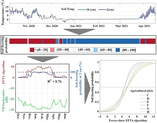
To overcome limitations identified in the Delta algorithm, particularly its reduced performance during transitional fall and spring seasons, a new 'exponential freeze-thaw algorithm' (EFTA) is introduced in this study. The proposed approach seeks to address the inherent limitations of the Delta algorithm and mitigate the challenge of overestimating frozen events during thawed periods. This is achieved by incorporating an exponential decay function that decreases the influence of backscatter fluctuations during the expected thawed periods in the shoulder seasons, while enhancing those during the expected frozen period. The concept behind the formulation of the EFTA derives from findings obtained from radar signal analysis research, especially studies on L-, C-, and X-band data [51,52], which highlight the effect of soil surface roughness on radar signals. The algorithm selectively incorporates quantitative aspects from these studies, but it does not directly model the relationship between radar signals and surface roughness. The EFTA is represented by the following equation:
where the expression denotes an exponential decay function, ensuring that the outcome remains constrained within the range of 1 to 0. The binary parameter K represents the expected thaw (K = 1) and frozen period (K = 0), which are, respectively, defined by the most negative and positive differences between radar signals at time t and at the preceding time (t − 1). The operationalization of this approach involves setting K to zero within the range defined by the most negative backscatter difference observed before February and the most positive backscatter difference observed after February. Conversely, K is assigned a value of 1 for radar signals occurring before the most negative backscatter differences in fall and after the most positive backscatter differences in spring, signifying the anticipated thaw periods. An example of the approach used to identify the soil freezing and thawing transitions in backscatter signals in the EFTA method is given in Supplementary Material Figure S3.
The EFTA was applied on both VH backscatter (VHEFTA) and VV (VVEFTA) backscattering signals. This facilitates identifying the greater sensitivity of either VV or VH polarizations to surface roughness in the context of freeze–thaw prediction, thereby evaluating their effectiveness in delivering essential information for forecasting freeze and thaw states. A greater positive value of EFTA corresponds to increased backscatter differences between the thawed references and the given date of interest under freezing conditions, which indicates a higher probability of freezing for the corresponding date.
2.6. Probabilistic Statistical Analysis
A generalized linear model (GLM), a statistical probabilistic method, was used to predict the freezing probability. To fit logistic regression models, the logit link function was used in the GLM to predict the freezing probability from potential predictors. The model was first applied to all instrumented plots across the two study sites and for the two studied years. By fitting the GLM model on the combined dataset, we could first evaluate the overall significance of the potential predictors and compare their effectiveness in predicting freezing probability for the agricultural plots.
In GLMs, Pseudo-R2 fit statistics are calculated using maximum likelihood estimates. Higher values of Pseudo-R2 indicate that the model explains more of the variance of the observed data. The Akaike Information Criterion (AIC) was used as a model comparison metric, allowing us to evaluate the relative quality of the different candidate statistical models of soil freezing probability. The AIC takes into account both the goodness of fit and the complexity of the model. The model with the lowest AIC value is considered the best fit among the candidate models.
We then added plot-level potential predictors, including soil types, crop types, and crop residues, to examine the effect of different plot conditions on soil freezing predictions in agricultural plots. The six candidate models tested can be classified into three categories based on their increasing complexity, starting with a global (i.e., on the combined datasets) GLM model (model 1), a mixed GLM model with a random effect on plots (model 2), and mixed models including plot-level predictors, cross-level interactions (interactions between time-dependent VHEFTA and spatially variable plot conditions), and a plot random effect (models 3 to 6).
- Soil freezing probability ~ 1 + VHEFTA;
- Soil freezing probability ~ 1 + VHEFTA + (1|Plot);
- Soil freezing probability ~ 1 + VHEFTA × Soil types + (1|Plot);
- Soil freezing probability ~ 1 + VHEFTA × Crop types + (1|Plot);
- Soil freezing probability ~ 1 + VHEFTA × Soil types + VHEFTA × Crop types + (1|Plot);
- Soil freezing probability ~ 1 + VHEFTA × Soil types + VHEFTA × Crop types + VHEFTA × Crop residues + (1|Plot).
Within the framework of mixed models, we calculated marginal and conditional R2 to discern the contributions of fixed and random effects. Marginal R2 in this context quantifies the variance explained by fixed effects, while conditional R2 takes into account both fixed and random effects, clarifying the proportions of variation attributed to each [44].
2.7. Model Calibration and Validation
Spatial and temporal cross-validation was used to evaluate the ability of the calibrated models to transpose between years and between plots. For temporal validation, the chosen model was calibrated on the first (2020–21) year and validated on the second year (2021–22). Then, the procedure was repeated after inverting the calibration and validation years.
For spatial cross-validation, we utilized a leave-one-out cross-validation (LOOCV) approach, incorporating data from both the 2020–21 and 2021–22 study years. This method involved evaluating the model’s performance by systematically excluding the data of one plot at a time from the calibration process, followed by testing the model on these excluded data. With 14 plots and data spanning 2 consecutive years, this approach resulted in 28 unique folds (14 plots each evaluated across 2 years). Data from each plot, whether from the first or second year of the study, were successively removed from the calibration dataset and used as a test sample. This comprehensive strategy ensured a rigorous assessment of the model’s performance across all agricultural plots.
The Brier score, mean absolute error (MAE), and R2 were employed to assess model accuracy, prediction errors, and goodness of fit during cross-validation. The Brier score is specifically used in the context of probabilities. A Brier score of 0 indicates perfect accuracy, reflecting precise alignment between the model’s forecasts and observed data, while a score of 1 signifies perfect inaccuracy [53]. In this research, we conducted statistical analysis and formulated our results using RStudio version 2022.07.2 Build 576, developed by RStudio, PBC, ©2009–2022.
3. Results
3.1. Observed FT Spatiotemporal Variability
The near-surface (2 cm) soil freezing probability displays variability between the two studied sites, monitored plots, and years (Figure 3). In both study sites, the observed probability of soil freezing in forest plots (A and B) demonstrated significantly fewer instances of freezing, despite experiencing a high frequency of FT transitions, compared to agricultural plots. The agricultural plots in St-Maurice (Figure 3c,d) experienced a prolonged duration of frozen conditions in comparison to St-Marthe (Figure 3a,b). While there is spatial variation in freezing probability within both agricultural and forest plots, temporal variations in freezing probability are also apparent during the two study periods at both sites. Spatial heterogeneity in frozen probability was observed within both agricultural and forest plots across the study site.
In St-Marthe, the forest plots (A and B) displayed notable spatial heterogeneity, marked by more frequent freeze–thaw transitions (Figure 3a,b). Meanwhile, the agricultural plots located near the forest edges (C and D) in the same vicinity were less frozen and exhibited less variability, with fewer freeze–thaw transitions. In these plots, only a few isolated freezing events with a freezing probability exceeding 80% were observed during the two study periods. This occurrence can be primarily attributed to the insulating properties of snow cover, especially prevalent in areas near the forest edge. The dense accumulation of snow in these plots forms a significant thermal layer, providing effective insulation against soil freezing. However, during the second study period, as depicted in Figure 3d, these agricultural plots exhibited an increased frequency of freezing and thawing transitions (C, D, and E plots). This phenomenon can be attributed to the spatial and temporal variability of snow depth, particularly the redistribution of snow, which affects its insulating properties at these plots. For a detailed depiction of spatial and temporal variations in freezing probability at 10 cm for all agro-forested plots at both sites, refer to Supplementary Material Figure S4.
3.2. Comparisons of Predictors for Modelling Freezing Probability
We conducted a comparative analysis using the logistic linear model to assess the performance of the EFTA, Delta, and FTI algorithms derived from VV and VH backscattering in explaining soil freezing probabilities at 2 cm and 10 cm soil depth. The results of this analysis are summarized in Table 2. In the context of modeling soil freezing probabilities, the AIC scores reflect the complexity and fit of the models at different soil depths. At a depth of 10 cm, where freezing probabilities trend towards thawing (indicated by probabilities tending to 0), the model exhibits a lower AIC score, adequately fitting the model due to more frequent thawing events. Thus, the variation in AIC scores between depths underscores the importance of tailoring model complexity to the specific characteristics and dynamics of soil freezing at different depths. According to the findings presented in Table 2, the logistic model utilizing the EFTA derived from VH polarization demonstrated better performance in predicting ground temperature observations at 2 cm, as indicated by its higher Pseudo-R2 value of 0.54. Furthermore, the predictions generated by the EFTA display a stronger ability to accurately predict frozen soil states across different soil depths and polarizations, outperforming both the Delta and FTI algorithms. As a result, further models were developed using the EFTA derived from VH backscattering.
For the comparative analysis of EFTA and Delta algorithms, Figure 4 depicts multiple plots illustrating the outcomes of both algorithms for the two study plots. As depicted in the upper plots of Figure 4, the Delta freeze–thaw algorithm effectively identified frozen states during winter when backscatter consistently remained low, distinguishing them from thawed periods. However, a significant challenge arose when encountering substantial drops in backscatter during the thawed periods in fall (early October to mid-October) and spring (mid-May to mid-June). In most plots, we observed one or two consecutive sudden drops in backscatter, particularly during mid-May to mid-June. Based on the time series of daily precipitation and air temperature presented in Supplementary Material, Figure S5, this phenomenon appears to be linked to a lack of rainfall over several weeks. This was evident during early fall (early October to mid-October) and, more notably, at the end of spring (mid-May to mid-June). The combination of no precipitation and rising air temperatures during these periods led to increasingly dry soil conditions, which preceded the sudden backscatter drops observed at the two study sites. In these instances, the Delta algorithm inaccurately identified these thawed events as frozen states, while the probability of soil freezing indicates non-frozen conditions. This misidentification of thawed conditions, observed across all plots, was attributed to the decrease in backscatter. Consequently, the proposed EFTA, illustrated in the lower plots of Figure 4, overcomes this limitation and brings a notable improvement in freeze–thaw state detection across all plots and years. This enhancement is apparent in the coefficient of determination (R2) between the predicted and observed probability of freezing at 2 cm.
3.3. Spatially Variable Probabilistic Modelling of FT Detection
Figure 5 illustrates examples of locally (at each plot) fitted logistic models, depicting the 2 cm depth observed freezing probability against VHEFTA. This representation aims to showcase the spatial and temporal variability of frozen soil between the plots. The fitted logistic regression model exhibited distinct Pseudo-R2 values for each agricultural or forest plot in each study period (Figure 5). Specifically, the H agricultural plot in St-Marthe (Figure 5a) displayed a higher goodness of fit in the first study year compared to the second year. This plot, characterized by clay soil type and soybean residues, had Pseudo-R2 values of 0.59 and 0.47 in the first (green curve) and second (sky blue curve) study years, respectively. In the agricultural plot I, the fitted logistic model showed a more robust correlation in the second year, marked by a ploughed crop type and scattered debris (Pseudo-R2: 0.57), compared to the first year of the study (Pseudo-R2: 0.48), as illustrated in Figure 5b. The presence of soybean debris and scattered crop residues in the plots may affect surface roughness. This roughness variability, in turn, influences the interaction of VH polarization with the surface.
Despite the consistent conditions observed across the two study years, the goodness of fit of the logistic model exhibited variations between these years in plots F and H at St-Maurice, as evidenced by the data presented in Table 2. The observed differences in model performance may be explained by other possible conditions, such as changes in other backscattering properties, changes in surface conditions, and variations in soil moisture content. These factors highlight the complexity of the interactions influencing radar signals and soil freezing dynamics within specific plots over time. The performance of the fitted GLM in predicting soil freezing probabilities varied across the different forest plots. Generally, the model exhibited lower efficacy in forest plots compared to agricultural plots across the two study sites. Notably, in the second year of the study, the highest correlation was observed in St-Marthe’s B forest plot, with Pseudo-R2 values reaching 0.58.
The mixed modelling approach, as outlined in Section 2.6, accommodates spatial variability. An analysis and comparison of the various candidate probabilistic models are presented in Table 3. As indicated in Table 3, the more complex mixed models, accounting for both fixed and random effects, explain relatively high variances in site-level predictors. However, it is noteworthy that the full complex model (Model 6) exhibits a lower level of performance compared to its fewer complex counterparts (Models 4 and 5).
The model results reveal that Model 4, a mixed model incorporating the interaction between VHEFTA and crop types (‘Crop-Mixed’ model) with a random effect on plots, displays a low AIC (231) and the highest marginal/conditional R2 values (0.59/0.61). Hence, the Crop-Mixed model accounts for 61% of the variance of observed soil freezing probability (conditional R2), of which 59% is attributed to fixed effects (marginal R2) and only 2% to random (plot) effects.
This model provides the most precise and parsimonious model to predict freezing probability, taking into account fixed (crop-type) and random (plot) spatial variability in agricultural plots. Table 4 provides a comprehensive overview of predictor effects derived from the Crop-Mixed model, showing their impact on soil freezing probabilities at the plot level. Notably, the p values associated with each predictor highlight the significant influence of EFTA derived from VH backscatter on model predictions.
While the main effects of crop types on soil freezing were not individually significant, the substantial interactions between crop types and VH backscatter signals underscore that the type of crop present modulates the VH backscatter response to soil freezing. Specifically, ploughed fields, as well as potato and soybean fields, exhibited the most pronounced modulating effects, with an interaction term estimate of 0.06. This was followed by maize with an estimate of 0.04, and grassland fields which served as the reference category with an estimate of 0. These findings indicate the presence of a ‘cross-over interaction’, where the influence of VHEFTA on soil freezing probabilities is not uniform across all crop types.
In Figure 6, cross-over interactions between different crop types and the relationship with VHEFTA regarding the predicted soil freezing probability are depicted. The data indicate that with rising VHEFTA values, there is a correspondingly increased probability of soil freezing across all crop types, although this trend occurs at varying rates for each type. For crop types such as ploughed fields, potatoes, and soybeans, the slopes indicate that the effect of VHEFTA on soil freezing probability is relatively stable across these crop types. However, the magnitude of the effect varies.
3.4. Model Validation
The results of the temporal cross-validation for the Crop-Mixed soil freezing model are presented in Table 5. The results indicated that the model performed more effectively when calibrated with the first year’s data and validated against the data from the subsequent year of the study. This effectiveness was evidenced by a robust squared correlation coefficient (R2) value of 0.60, a low Mean Absolute Error (MAE) of 0.18, and a Brier score of 0.19, which collectively indicate moderately high performance by the model.
The leave-one (plot)-out spatial cross validation (LOOCV) yielded a mean R2 score of 0.79, along with small MAE and Brier scores of 0.14 and 0.17, respectively (Figure 7), suggesting a good spatial transferability of the model. The lowest R2 observed was for St-Marthe’s C plot in 2020–21, indicating that the model’s predictions are comparatively less precise for this plot than for others.
When considering the average cross-validation R2 values from the first and second years of the study, a higher R2 of 0.60 is observed for 2021–22 compared to an R2 of 0.55 for 2020–21. This implies that the model, when trained using all available data while excluding the specific plot in the second year under consideration, more effectively identifies the freeze–thaw predictions.
The comparison between predicted and observed 2 cm depth soil freezing probability shows significant scatter, without any clear relationship with crop types (Figure 8a). The good performance of the model is thus partly due to the clustering of values at low and high probabilities, i.e., the model is able to discriminate between thawed and frozen conditions but yields more uncertain predictions at intermediate probabilities. To evaluate the ability of the model to classify the observed freezing probabilities into ‘frozen’ or ‘thawed’ conditions, the predicted and observed freezing probabilities were converted into binary states of frozen and thawed using a threshold of 0.5. The model accurately predicted the frozen status with an overall accuracy of 85.2%, confirming that it successfully classified most freezing and thawing events in agricultural plots across two sites over two study periods (Figure 8b). The classification accuracy varied among crop types, with grassland plots showing the highest classification accuracy (96%), followed by soybeans (86%), ploughed fields (83%), maize (82%), and potatoes (80%). In plots C and D of St-Marthe, which are grassland areas, a predominantly thawed state was observed, as depicted in Figure 3a,b. This thawed state represented the majority class in these specific plots. Consequently, the model demonstrated high classification accuracy, particularly in identifying this prevalent thawed condition. The ability of the model to accurately classify the more common thawed states contributed significantly to its overall effectiveness in these grassland areas.
4. Discussion
4.1. FT Spatial and Temporal Variability
By the analysis of spatial and temporal variations in soil freezing probability, derived from soil temperature measurements at 2 cm depth, we have noted considerable variations in freezing probability among the plots of study sites (Figure 3). This variability is evident regardless of whether the plots are situated in agricultural or forested areas. The primary likely factors contributing to this variability are the spatial and temporal variations in local plot attributes, including variations in soil properties, vegetation cover, and snow depth conditions across the study sites.
As compared to agricultural plots, forested areas in St-Marthe and St-Maurice exhibit fewer freezing occurrences, which can be attributed to the substantial amount of forest litter acting as an insulating barrier between the soil and the air [54]. This insulation effectively reduces heat loss from the soil, thereby impeding rapid freezing. Additionally, the attenuated winds in forested areas can further reduce sensible heat loss through turbulent fluxes. Moreover, the presence of trees contributes to ground heating through longwave radiation [55].
Ground-based measurements of snow depth in St-Maurice over two study periods reveal that forest plots (plots A and B) typically display the highest snow depths. This is largely due to the forest canopies’ ability to intercept snowfall, which leads to greater accumulation in the forest. Additionally, the canopy cover provides protection against direct sunlight and wind, mitigating snow sublimation. As shown in Figure 3c, the most events of soil freezing in 2020–21 occurred in forest plot B in St-Maurice, with the lowest recorded snow depths (see Supplementary Material Figure S6).
In contrast, agricultural plots demonstrated notable temporal variability in snow depth, with the first study year showing relatively higher snow accumulation. This may explain the rather shorter duration of soil freezing experienced by the agricultural plots in the first study period compared to the second year. Despite all agricultural plots in St-Maurice being sufficiently far from forest edges, there was also spatial variability in snow depth between plots.
Figure 3 illustrates that the agricultural plots in St-Maurice experienced extended periods of soil freezing during the two study periods, compared to the relatively shorter freezing durations observed in St-Marthe’s agricultural plots. Despite variations in spatial and temporal snow cover, factors such as soil properties and climate conditions significantly influenced the duration of soil freezing in St-Maurice compared to St-Marthe. Notably, the soil composition differs between these locations, with predominantly clay soil in St-Marthe and silty clay in St-Maurice. Clay, being a finer-textured soil, contrasts with the more coarse-textured silty clay. According to Jagtar Bhatti et al. [56], fine-textured soils have a larger mineral surface area and a more extensive network of fine pores. These characteristics impede ice formation, primarily restricting it to larger pore spaces. Consequently, fine-textured soils are more likely to experience super-cooling, remaining unfrozen or partially unfrozen even under sub-zero temperatures. This phenomenon is less pronounced in coarser-textured soils, such as the silty clay found in St-Maurice, which explains the longer and more intense soil freezing observed there compared to St-Marthe. On the other hand, the average daily air temperature during the two study periods for St-Marthe and St-Maurice was 3.07 °C and 2.10 °C, respectively (see Supplementary Material Figure S5). The data indicate that, during the two study periods, St-Maurice was approximately one °C colder than St-Marthe. The higher latitude of St-Maurice compared to St-Marthe could be a contributing factor to this temperature difference, which in turn may influence the extent of soil freezing.
Regarding the variation in soil freezing occurrences among plots, complex interactions among plot-level variables can play a considerable influence. For instance, the F plot in St-Marthe during 2021–22 displayed prolonged soil freezing events compared to the F plot in 2020–21, despite having identical site conditions (Figure 4). A key factor under consideration is the variability in snow cover across the two study years. Freeze–thaw events are highly dependent on both snow depth and soil temperature. Decker et al. [57] observed that in snow-free plots, there was a significant negative correlation between the average ambient temperature and the number of days the soil remained frozen at various soil depths. This finding is particularly relevant to our study, given the absence of in situ snow depth data for the plots. A plausible explanation for the more prolonged soil freezing observed in the second year might be linked to the differences in average daily air temperatures during the two periods. The 2020–21 study year had an average temperature of 3.73 °C, while the subsequent 2021–22 year recorded a lower average temperature of 2.41 °C (see Supplementary Material Figure S5a). This relatively lower average temperature in the second year likely led to more severe soil-freezing episodes.
4.2. Retrieving Ground Frozen State from VH Backscatter
When it comes to the S1 polarization ability to predict frozen soil, better model performances were obtained when using VH backscatter signals within the EFTA logistic models to predict 2 cm depth soil freezing probability. This can be explained by the increased sensitivity of cross-polarized VH backscatter to surface characteristics (soil roughness, soil types, ground vegetation density, soil state) [58]. Further, as compared to VV polarization, VH backscattering correlates more strongly with soil water content [59]. Irrespective of the algorithm employed, the model predictions exhibited a more suitable goodness of fit for soil freezing at a depth of 2 cm. Due to the limited penetration depth of the C-band backscattered SAR signal, its sensitivity to dielectric variations decreases with increasing depth of the frozen soil, thereby making the prediction of frozen soil less reliable for deeper layers compared to the near-surface [60]. Furthermore, the dielectric discontinuity between soil and air results in distinct radar backscattering coefficients, making the signal particularly sensitive to soil freezing near the surface [61,62]. The improved performance of the probabilistic approach employing the suggested EFTA derived from VH radar data (Pseudo-R2 = 0.54) indicates its enhanced capability to detect variations in backscatter during frozen and thawed episodes (Table 2).
4.3. GLM Prediction and Influencing Variables on Radar Signals
In St-Marthe, during both study years, the locally fitted GLM results indicated that the H plot showed improved model performance in the first year compared to the second one, despite sharing similar soil types (Figure 5a). A plausible explanation for this phenomenon is the presence of crop debris on the surface during fall, which contributes to a significant impact on radar backscattering through two primary mechanisms. Firstly, it introduces additional roughness to the soil surface, thereby influencing the scattering of radar waves. Secondly, the debris assists in retaining soil moisture, thereby altering the soil dielectric constant and modifying the interaction between the radar signal and the ground.
Generally, the different GLM model performances observed between agricultural plots in the two study periods (Figure 5a,b,d,e) can largely be attributed to several interconnected aspects. Firstly, the local variability in snow depth, influenced by microtopographic variations, differing vegetation covers, and wind patterns across sites in St-Marthe and St-Maurice [63], significantly impacts the ground’s thermal regime. These changes in ground surface temperature within the plots result in alterations to the soil’s freezing and thawing state. Secondly, even minor changes in soil moisture content can notably alter the soil’s complex permittivity [64], a phenomenon that is particularly evident during fall and spring. During the thawing period, spatial and temporal variations in wet soil across different plots independently affect the VH radar. An increase in soil moisture correlates with a rise in the backscattering coefficient. This complex interplay between local snow depth variability and soil moisture dynamics is crucial for understanding the varied backscatter response and, consequently, the differing model performances in agricultural plots across distinct study periods.
The logistic model fitted to the forest plots indicated higher performance in cases where the plots exhibited a relatively balanced distribution of frozen and thaw events (Figure 5c: 2021–22). This balance contributed to more accurate predictions. Specifically, the forest plot A in St-Maurice experienced only a limited number of frozen episodes over the two study years. In such instances, the lower predictive performance for frozen states is maintained, as the imbalanced dataset biases the model’s predictions toward the dominant class, which is the thaw state. This highlights the significance of having a sufficiently extensive and balanced training dataset for model calibration and validation. Mixed models are well-suited for this purpose as they enable fitting the model on the whole dataset, accounting for spatial variabilities through plot-level predictors, cross-level interactions, and random effects.
4.4. Crop-Mixed Model and Predictor Effects
The results revealed that among the tested mixed models, the Crop-Mixed model, incorporating the interplay between VHEFTA and crop type predictors, exhibited the most favorable performance among the candidate models. Additionally, the Crop-Mixed model brought to light discernible effects of predictors, including cross-level interactions between VHEFTA and crop types which improved the prediction of soil freezing probability (Table 3). Accordingly, the obtained conditional R2 of 0.61 emphasizes the collective effect of both fixed and random effects in explaining the variability within the dependent variable.
The analysis revealed that while the inclusion of crop-type interactions improved the model’s predictions, this improvement remains relatively small compared to the Model 2 results, which only considered random effects. A significant observation is the absence of random variability in the Crop-Mixed model, as indicated by a τ00 Plot value of 0.00 (Table 4). This finding suggests that the incorporation of crop types effectively explained the random variability, which was more pronounced in the model featuring only random effects.
Comparatively, the analysis of Model 2, detailed in Table 3, provided insightful results. There was minimal spatial variability between plots based on the closeness of the conditional R2 (0.56) and marginal R2 values (0.57) in this model. This suggests that, while random effects are indeed present, they do not significantly contribute to the variability in soil freezing probability across different plots. This highlights the importance of cross-level interaction in the Crop-Mixed model, where crop types modulate the backscatter response to soil freezing. Accordingly, the results of cross-over interactions among different crop types demonstrated varied relationships between VHEFTA and the predicted probability of soil freezing. Specifically, ploughed fields, as well as potato and soybean fields, showed an increased susceptibility to soil freezing across all VHEFTA values. Conversely, grasslands typically exhibited a lower predicted probability of soil freezing in response to changes in VHEFTA, compared to other crop types. These variations underscore the significant influence of specific crop types on the prediction of soil freezing.
The temporal variability of the VHEFTA at the plot-level offers insight into the varying results of temporal cross-validation. Despite the consistent soil types and similar crop types across the agricultural plots, the differences in snow depth and air temperature across the two study periods are notable. The presence of the relatively higher snow depth in agricultural plots (see Supplementary Material Figure S6) and higher average air temperatures during the first year (see Supplementary Material Figure S5) potentially account for the improved performance of the Crop-Mixed model’s temporal cross-validation compared to the second year (Table 5). Specifically, these conditions are possibly key drivers that significantly influence the probability of soil freezing. Furthermore, the results of spatial cross-validation for the Crop-Mixed model (Figure 7) emphasize the importance of accounting for the spatial heterogeneity of snow cover in plots, as well as the complexities of surface roughness in different agricultural plots, when developing predictive models for soil freezing in farmlands. The observation of very limited soil freezing events for St-Marthe’s C and D plots in the 2020–21 period and apparently no freezing events in the 2021–22 period near the forest edge, as indicated in Figure 3a,b, can be scientifically explained by the presence of high snow depth in these areas.
In this study, a novel freeze–thaw algorithm, the EFTA, was developed specifically for agro-forested areas where seasonal freeze–thaw transitions are dominant. The developed EFTA demonstrated significantly improved results compared to both Delta (Table 2 and Figure 4) and FTI methods (Table 2). However, future research should consider certain limitations, particularly the effects of high backscatter noise before the onset of the frozen period and during the onset of snow melting in spring. To address these challenges, it is advisable to experiment with identifying the potential frozen period by selecting the most negative and positive backscatter differences before and after the frozen period, while excluding months with a high probability of thawing (e.g., June and later). As a result, the algorithm performance will improve in situations with significant backscatter noise. Additionally, for study sites with limited frozen conditions, fine-tuning the K parameter becomes essential to align the algorithm’s output with the specific conditions of the study site, thereby enhancing its adaptability and robustness.
5. Conclusions
This study represents a new application of a probabilistic approach for identifying locally frozen soil conditions in agro-forested environments in southern Québec, Canada, using Sentinel-1 SAR observations. The utilization of the GLM proved to be a robust statistical framework for analyzing soil freezing probability and conducting spatially variable probabilistic modeling of freeze–thaw detection. Through the incorporation of mixed models, this study significantly advanced our understanding of freeze–thaw dynamics and enabled more precise and spatially explicit predictions within the study area. Notably, the Crop-Mixed model demonstrated a superior ability to capture the variability of site-level predictors for freezing probability, emphasizing the advantages of employing the VHEFTA and the mixed model approach. These methods offer enhanced accuracy and explanatory power in predicting the probability of freezing in mixed agro-forested areas. In light of the results, the newly developed EFTA has shown capability in detecting frozen and thawed states in both agricultural and forested areas. The results underscore the importance of a deeper comprehension of spatial and temporal dynamics in radar signal interactions with surfaces, providing valuable insights for optimizing model calibration and validation strategies of soil freezing retrieval models in contexts where surface conditions exhibit seasonal variations.
Supplementary Materials
The following supporting information can be downloaded at: https://www.mdpi.com/article/10.3390/rs16071294/s1, Figure S1: Schematic representation of the measurement configuration for soil temperature measurements (2 cm and 10 cm depths), aligned with the Sentinel 1 pixel size of 10 m. The geometry of the configuration includes five soil pits (blue points) arranged in a cross shape with a distance of 5 m between each pit; Figure S2: Correction of local incidence angles in St-Maurice’s C plot with the corresponding linear equation. (a) VH backscatter before correction in 2020–21. (b) The corrected VH backscatter in 2020–21. (c) VH backscatter before correction in 2021–22. (d) The corrected VH backscatter in 2021–22; Figure S3: Examples of the approach used to identify the soil freezing and thawing transitions in backscatter signals in the of the EFTA method. The most negative backscatter differences (upward green triangles) before February represents the most probable onset of the freezing period (delineated in light blue), while the most positive difference (downward green triangles) after February represent the most probable onset of soil thawing (delineated in light red). (a–d) correspond to St-Marthe’s I and J plots and St-Maurice’s G and H plots, respectively, for the year 2020–21. (e–h) correspond to St-Marthe’s I and J plots and St-Maurice’s G and H plots, respectively, for the year 2021–22; Figure S4: Spatial and temporal variations in freezing probability (10 cm) along with corresponding the S1 overpass for all agro-forest plots in St-Marthe. (a,b) FT variations based on freezing probability in St-Marthe’s plots over two study periods (2020–21 and 2021–22). (c,d) FT variations based on freezing probability in St-Maurice’s plots over two study periods (2020–21 and 2021–22). In each site, forest plots are represented by A and B plots (green rectangle). For St-Marthe’s J and I and St-Maurice’s F, G, and H plots, the initiation of soil temperature monitoring started later, resulting in an absence of freezing probability values; Figure S5: Time series plot of daily precipitation and air temperature, October 2020 to June 2022, for two study sites. (a) St-Marthe. (b) St-Maurice. Note: the average daily air temperatures for the entire study period, as well as for the first and second years (October to June), were calculated for both St-Marthe and St-Maurice; Figure S6: Average snow depth (meters) in agro-forested plots of St-Maurice over two study years in 2020–21 and 2021–22. Plot classification: ‘A’ and ‘B’ as forest plots; ‘C’ to ‘H’ as agricultural plots. Measurement period: End of November to March each year. Method: Using snow ruler, snow depth recorded at five points within a 5m × 5m square per plot, including a central point. Calculation: Average of five measurements per plot, aggregated to represent overall snow depth for each plot.
Author Contributions
Conceptualization, C.K. and A.R.; methodology, C.K., A.R., and S.T.; formal analysis, S.T., C.K., and A.R.; data curation, S.T.; writing—original draft preparation, S.T.; writing—review and editing, C.K. and A.R.; supervision, C.K. and A.R.; project administration, C.K. and A.R.; funding acquisition, C.K. and A.R. All authors have read and agreed to the published version of the manuscript.
Funding
This study was financially supported by Fonds de Recherche du Québec Nature et Technologies (FRQNT) under the Merit scholarship program for foreign students (PBEEE) program for doctoral research scholarships (File number: 275403), Canadian Space Agency FAST (19FAQCTB19), and the FRQNT Team Research Project grant 2022-PR-299776 (C. Kinnard).
Data Availability Statement
The datasets utilized in this study are publicly available in the Borealis repository at the following link: https://doi.org/10.5683/SP3/LGLCKW, accessed on 1 April 2024.
Acknowledgments
The authors extend their appreciation to the members of GlacioLab for their help during our fieldwork.
Conflicts of Interest
The authors declare no conflicts of interest.
References
- Henry, H.A.L. Soil Freeze–Thaw Cycle Experiments: Trends, Methodological Weaknesses and Suggested Improvements. Soil. Biol. Biochem. 2007, 39, 977–986. [Google Scholar] [CrossRef]
- Zhang, T.; Armstrong, R.L.; Smith, J. Investigation of the Near-surface Soil Freeze-thaw Cycle in the Contiguous United States: Algorithm Development and Validation. J. Geophys. Res. Atmos. 2003, 108, D22. [Google Scholar] [CrossRef]
- McDonald, K.C.; Kimball, J.S.; Zhao, M.; Njoku, E.; Zimmermann, R.; Running, S.W. Spaceborne Microwave Remote Sensing of Seasonal Freeze-Thaw Processes in the Terrestrial High Latitudes: Relationships with Land-Atmosphere CO2 Exchange. In Microwave Remote Sensing of the Atmosphere and Environment IV; International Society for Optics and Photonics: Bellingham, WA, USA, 2004; Volume 5654, pp. 167–178. [Google Scholar]
- Gao, C.; Bai, W.; Wang, Z.; Wu, X.; Liu, L.; Deng, N.; Xia, J. Simulations and Analysis of GNSS Multipath Observables for Frozen and Thawed Soil under Complex Surface Conditions. Water 2021, 13, 1986. [Google Scholar] [CrossRef]
- Walvoord, M.A.; Kurylyk, B.L. Hydrologic Impacts of Thawing Permafrost—A Review. Vadose Zone J. 2016, 15, vzj2016- 01. [Google Scholar] [CrossRef]
- Wang, J.; Luo, S.; Li, Z.; Wang, S.; Li, Z. The Freeze/Thaw Process and the Surface Energy Budget of the Seasonally Frozen Ground in the Source Region of the Yellow River. Theor. Appl. Clim. 2019, 138, 1631–1646. [Google Scholar] [CrossRef]
- Krogstad, K. Impact of Winter Soil Processes on Nutrient Leaching in Cold Region Agroecosystems. Master’s Thesis, University of Waterloo, Waterloo, ON, Canada, 2021. [Google Scholar]
- Cober, J.R.; Macrae, M.L.; Van Eerd, L.L. Nutrient Release from Living and Terminated Cover Crops under Variable Freeze–Thaw Cycles. Agron. J. 2018, 110, 1036–1045. [Google Scholar] [CrossRef]
- Edwards, L.M. The Effects of Soil Freeze–Thaw on Soil Aggregate Breakdown and Concomitant Sediment Flow in Prince Edward Island: A Review. Can. J. Soil. Sci. 2013, 93, 459–472. [Google Scholar] [CrossRef]
- Leuther, F.; Schlüter, S. Impact of Freeze–Thaw Cycles on Soil Structure and Soil Hydraulic Properties. Soil 2021, 7, 179–191. [Google Scholar] [CrossRef]
- Wang, K.; Zhang, T.; Zhong, X. Changes in the Timing and Duration of the Near-Surface Soil Freeze/Thaw Status from 1956 to 2006 across China. Cryosphere 2015, 9, 1321–1331. [Google Scholar] [CrossRef]
- Guo, D.; Wang, H. Simulated Change in the Near-Surface Soil Freeze/Thaw Cycle on the Tibetan Plateau from 1981 to 2010. Chin. Sci. Bull. 2014, 59, 2439–2448. [Google Scholar] [CrossRef]
- Peng, X.; Frauenfeld, O.W.; Cao, B.; Wang, K.; Wang, H.; Su, H.; Huang, Z.; Yue, D.; Zhang, T. Response of Changes in Seasonal Soil Freeze/Thaw State to Climate Change from 1950 to 2010 across China. J. Geophys. Res. Earth Surf. 2016, 121, 1984–2000. [Google Scholar] [CrossRef]
- Wang, R.; Zhu, Q.; Ma, H.; Ai, N. Spatial-Temporal Variations in near-Surface Soil Freeze-Thaw Cycles in the Source Region of the Yellow River during the Period 2002–2011 Based on the Advanced Microwave Scanning Radiometer for the Earth Observing System (AMSR-E) Data. J. Arid Land 2017, 9, 850–864. [Google Scholar] [CrossRef]
- Luo, S.; Wang, J.; Pomeroy, J.W.; Lyu, S. Freeze–Thaw Changes of Seasonally Frozen Ground on the Tibetan Plateau from 1960 to 2014. J. Clim. 2020, 33, 9427–9446. [Google Scholar] [CrossRef]
- Xu, G.; Huang, M.; Li, P.; Li, Z.; Wang, Y. Effects of Land Use on Spatial and Temporal Distribution of Soil Moisture within Profiles. Environ. Earth Sci. 2021, 80, 80. [Google Scholar] [CrossRef]
- Qin, Y.; Bai, Y.; Chen, G.; Liang, Y.; Li, X.; Wen, B.; Lu, X.; Li, X. The Effects of Soil Freeze–Thaw Processes on Water and Salt Migrations in the Western Songnen Plain, China. Sci. Rep. 2021, 11, 3888. [Google Scholar] [CrossRef] [PubMed]
- Li, Y.; Fu, Q.; Li, T.; Liu, D.; Hou, R.; Li, Q.; Yi, J.; Li, M.; Meng, F. Snow Melting Water Infiltration Mechanism of Farmland Freezing-Thawing Soil and Determination of Meltwater Infiltration Parameter in Seasonal Frozen Soil Areas. Agric. Water Manag. 2021, 258, 107165. [Google Scholar] [CrossRef]
- Cheng, Y.; Li, P.; Xu, G.; Li, Z.; Wang, T.; Cheng, S.; Zhang, H.; Ma, T. The Effect of Soil Water Content and Erodibility on Losses of Available Nitrogen and Phosphorus in Simulated Freeze-Thaw Conditions. Catena 2018, 166, 21–33. [Google Scholar] [CrossRef]
- Zhao, Y.; Li, Y.; Yang, F. Critical Review on Soil Phosphorus Migration and Transformation under Freezing-Thawing Cycles and Typical Regulatory Measurements. Sci. Total Environ. 2020, 751, 141614. [Google Scholar] [CrossRef] [PubMed]
- Roy, A.; Toose, P.; Williamson, M.; Rowlandson, T.; Derksen, C.; Royer, A.; Berg, A.A.; Lemmetyinen, J.; Arnold, L. Response of L-Band Brightness Temperatures to Freeze/Thaw and Snow Dynamics in a Prairie Environment from Ground-Based Radiometer Measurements. Remote Sens. Environ. 2017, 191, 67–80. [Google Scholar] [CrossRef]
- Shao, W.; Zhang, T. Assessment of Four Near-Surface Soil Freeze/Thaw Detection Algorithms Based on Calibrated Passive Microwave Remote Sensing Data Over China. Earth Space Sci. 2020, 7, e2019EA000807. [Google Scholar] [CrossRef]
- Rautiainen, K.; Lemmetyinen, J.; Pulliainen, J.; Vehvilainen, J.; Drusch, M.; Kontu, A.; Kainulainen, J.; Seppanen, J. L-Band Radiometer Observations of Soil Processes in Boreal and Subarctic Environments. IEEE Trans. Geosci. Remote Sens. 2011, 50, 1483–1497. [Google Scholar] [CrossRef]
- Derksen, C.; Xu, X.; Dunbar, R.S.; Colliander, A.; Kim, Y.; Kimball, J.S.; Black, T.A.; Euskirchen, E.; Langlois, A.; Loranty, M.M. Retrieving Landscape Freeze/Thaw State from Soil Moisture Active Passive (SMAP) Radar and Radiometer Measurements. Remote Sens. Environ. 2017, 194, 48–62. [Google Scholar] [CrossRef]
- Jin, R.; Zhang, T.; Li, X.; Yang, X.; Ran Antarctic, Y. Mapping Surface Soil Freeze-Thaw Cycles in China Based on SMMR and SSM/I Brightness Temperatures from 1978 to 2008. Arct. Antarct. Alp. Res. 2015, 47, 213–229. [Google Scholar] [CrossRef]
- Zhao, T.; Zhang, L.; Jiang, L.; Zhao, S.; Chai, L.; Jin, R. A new soil freeze/thaw discriminant algorithm using AMSR-E passive microwave imagery. Hydrol. Process. 2011, 25, 1704–1716. [Google Scholar] [CrossRef]
- Roy, A.; Toose, P.; Derksen, C.; Rowlandson, T.; Berg, A.; Lemmetyinen, J.; Royer, A.; Tetlock, E.; Helgason, W.; Sonnentag, O. Spatial Variability of L-Band Brightness Temperature during Freeze/Thaw Events over a Prairie Environment. Remote Sens. 2017, 9, 894. [Google Scholar] [CrossRef]
- Park, S.-E.; Bartsch, A.; Sabel, D.; Wagner, W.; Naeimi, V.; Yamaguchi, Y. Monitoring Freeze/Thaw Cycles Using ENVISAT ASAR Global Mode. Remote Sens. Environ. 2011, 115, 3457–3467. [Google Scholar] [CrossRef]
- Du, J.; Kimball, J.S.; Azarderakhsh, M.; Dunbar, R.S.; Moghaddam, M.; McDonald, K.C. Classification of Alaska Spring Thaw Characteristics Using Satellite L-Band Radar Remote Sensing. IEEE Trans. Geosci. Remote Sens. 2014, 53, 542–556. [Google Scholar]
- Dunbar, S.; Xu, X.; Colliander, A.; Derksen, C.; Kimball, J.; Kim, Y. Algorithm Theoretical Basis Document (ATBD) SMAP Level 3 Radiometer Freeze/Thaw Data Products (L3_FT_P and L3_FT_P_E); NASA Jet Propulsion Laboratory (JPL): Pasadena, CA, USA, 2016. [Google Scholar]
- Rodionova, N.V. Identification of Frozen/Thawed Soils in the Areas of Anadyr (Chukotka) and Belaya Gora (Sakha) from the Sentinel 1 Radar Data. Atmos. Ocean. Phys. 2019, 55, 1314–1321. [Google Scholar] [CrossRef]
- Fayad, I.; Baghdadi, N.; Bazzi, H.; Zribi, M. Near Real-Time Freeze Detection over Agricultural Plots Using Sentinel-1 Data. Remote Sens. 2020, 12, 1976. [Google Scholar] [CrossRef]
- Baghdadi, N.; Bazzi, H.; El Hajj, M.; Zribi, M. Detection of Frozen Soil Using Sentinel-1 SAR Data. Remote Sens. 2018, 10, 1182. [Google Scholar] [CrossRef]
- de Aguirre Escobar, A.M. Analysis of Surface Roughness in Agricultural Soils Using In-Situ Measurements and Remote Sensing Techniques. Ph.D. Thesis, Public University of Navarre, Universidad Pública de Navarra, Navarre, Spain, 2017. [Google Scholar]
- Hudier, E.; Gosseli, J.-S. Impact of Daily Melt and Freeze Patterns on Sea Ice Large Scale Roughness Features Extraction. In Geoscience and Remote Sensing New Achievements; IntechOpen: London, UK, 2010. [Google Scholar]
- Holah, N.; Baghdadi, N.; Zribi, M.; Bruand, A.; King, C. Potential of ASAR/ENVISAT for the Characterization of Soil Surface Parameters over Bare Agricultural Fields. Remote Sens. Environ. 2005, 96, 78–86. [Google Scholar] [CrossRef]
- Khaldoune, J.; Van Bochove, E.; Bernier, M.; Nolin, M.C. Mapping Agricultural Frozen Soil on the Watershed Scale Using Remote Sensing Data. Appl. Environ. Soil. Sci. 2011, 2011, 193237. [Google Scholar] [CrossRef]
- Rodionova, N.V. Correlation of the Sentinel 1 Radar Data with Ground-Based Measurements of the Soil Temperature and Moisture. Izv. Atmos. Ocean. Phys. 2019, 55, 939–948. [Google Scholar] [CrossRef]
- Dharmadasa, V.; Kinnard, C.; Baraër, M. An Accuracy Assessment of Snow Depth Measurements in Agro-Forested Environments by UAV Lidar. Remote Sens. 2022, 14, 1649. [Google Scholar] [CrossRef]
- Wackerly, D.D. Mathematical Statistics with Applications, 7th ed.; Thomson Brooks/Cole: Belmont, CA, USA, 2008. [Google Scholar]
- Gorelick, N.; Hancher, M.; Dixon, M.; Ilyushchenko, S.; Thau, D.; Moore, R. Google Earth Engine: Planetary-Scale Geospatial Analysis for Everyone. Remote Sens. Environ. 2017, 202, 18–27. [Google Scholar] [CrossRef]
- Torres, R.; Snoeij, P.; Geudtner, D.; Bibby, D.; Davidson, M.; Attema, E.; Potin, P.; Rommen, B.; Floury, N.; Brown, M. GMES Sentinel-1 Mission. Remote Sens. Environ. 2012, 120, 9–24. [Google Scholar] [CrossRef]
- Filipponi, F. Sentinel-1 GRD Preprocessing Workflow. In Proceedings of the International Electronic Conference on Remote Sensing, Vitrul, 22 May–5 June 2019; MDPI: Basel, Switzerland, 2019; p. 11. [Google Scholar]
- Domg, Y.; Milne, A.K. Toward edge sharpening: A SAR speckle filtering algorithm. IEEE Trans. Geosci. Remote Sens. 2001, 39, 851–863. [Google Scholar] [CrossRef]
- Lee, J.-S.; Wen, J.-H.; Ainsworth, T.L.; Chen, K.-S.; Chen, A.J. Improved Sigma Filter for Speckle Filtering of SAR Imagery. IEEE Trans. Geosci. Remote Sens. 2008, 47, 202–213. [Google Scholar]
- Amani, M.; Brisco, B.; Afshar, M.; Mirmazloumi, S.M.; Mahdavi, S.; Mirzadeh, S.M.J.; Huang, W.; Granger, J. A Generalized Supervised Classification Scheme to Produce Provincial Wetland Inventory Maps: An Application of Google Earth Engine for Big Geo Data Processing. Big Earth Data 2019, 3, 378–394. [Google Scholar] [CrossRef]
- Fuhrmann, T.; Garthwaite, M.C. Resolving Three-Dimensional Surface Motion with InSAR: Constraints from Multi-Geometry Data Fusion. Remote Sens. 2019, 11, 241. [Google Scholar] [CrossRef]
- Schaufler, S.; Bauer-Marschallinger, B.; Hochstöger, S.; Wagner, W. Modelling and Correcting Azimuthal Anisotropy in Sentinel-1 Backscatter Data. Remote Sens. Lett. 2018, 9, 799–808. [Google Scholar] [CrossRef]
- Rautiainen, K.; Lemmetyinen, J.; Schwank, M.; Kontu, A.; Ménard, C.B.; Mätzler, C.; Drusch, M.; Wiesmann, A.; Ikonen, J.; Pulliainen, J. Detection of Soil Freezing from L-Band Passive Microwave Observations. Remote Sens. Environ. 2014, 147, 206–218. [Google Scholar] [CrossRef]
- Touati, C.; Ratsimbazafy, T.; Poulin, J.; Bernier, M.; Homayouni, S.; Ludwig, R. Landscape Freeze/Thaw Mapping from Active and Passive Microwave Earth Observations over the Tursujuq National Park, Quebec, Canada. Écoscience 2021, 28, 421–433. [Google Scholar] [CrossRef]
- Zribi, M.; Sahnoun, M.; Baghdadi, N.; Le Toan, T.; Hamida, A.B. Analysis of the Relationship between Backscattered P-Band Radar Signals and Soil Roughness. Remote Sens. Environ. 2016, 186, 13–21. [Google Scholar] [CrossRef]
- Baghdadi, N.; King, C.; Bourguignon, A.; Remond, A. Potential of ERS and RADARSAT Data for Surface Roughness Monitoring over Bare Agricultural Fields: Application to Catchments in Northern France. Int. J. Remote Sens. 2002, 23, 3427–3442. [Google Scholar] [CrossRef]
- Brier, G.W. Verification of Forecasts Expressed in Terms of Probability. Mon. Weather. Rev. 1950, 78, 1–3. [Google Scholar] [CrossRef]
- Smith, M.W. Microclimatic Influences on Ground Temperatures and Permafrost Distribution, Mackenzie Delta, Northwest Territories. Can. J. Earth Sci. 1975, 12, 1421–1438. [Google Scholar] [CrossRef]
- Pomeroy, J.W.; Marks, D.; Link, T.; Ellis, C.; Hardy, J.; Rowlands, A.; Granger, R. The Impact of Coniferous Forest Temperature on Incoming Longwave Radiation to Melting Snow. Int. J. 2009, 23, 2513–2525. [Google Scholar] [CrossRef]
- Jagtar Bhatti, V.B.; Mark Castonguay, R.E.; Arp, P.A. Modeling Snowpack and Soil Temperature and Moisture Conditions in a Jack Pine, Black Spruce and Aspen Forest Stand in Central Saskatchewan (BOREAS SSA). Can. J. Soil. Sci. 2006, 86, 203–217. [Google Scholar] [CrossRef]
- Decker, K.L.M.; Wang, D.; Waite, C.; Scherbatskoy, T. Snow Removal and Ambient Air Temperature Effects on Forest Soil Temperatures in Northern Vermont. Soil. Sci. Soc. Am. J. 2003, 67, 1234–1242. [Google Scholar] [CrossRef]
- Bauer-Marschallinger, B.; Cao, S.; Navacchi, C.; Freeman, V.; Reuß, F.; Geudtner, D.; Rommen, B.; Vega, F.C.; Snoeij, P.; Attema, E. The Normalised Sentinel-1 Global Backscatter Model, Mapping Earth’s Land Surface with C-Band Microwaves. Sci. Data 2021, 8, 277. [Google Scholar] [CrossRef] [PubMed]
- Soudani, K.; Delpierre, N.; Berveiller, D.; Hmimina, G.; Vincent, G.; Morfin, A.; Dufrêne, É. Potential of Synthetic Aperture Radar Sentinel-1 Time Series for the Monitoring of Phenological Cycles in a Deciduous Forest. bioRxiv 2021. [Google Scholar] [CrossRef]
- Asmuß, T.; Bechtold, M.; Tiemeyer, B. On the Potential of Sentinel-1 for High Resolution Monitoring of Water Table Dynamics in Grasslands on Organic Soils. Remote Sens. 2019, 11, 1659. [Google Scholar] [CrossRef]
- Rowlandson, T.L.; Berg, A.A.; Roy, A.; Kim, E.; Lara, R.P.; Powers, J.; Lewis, K.; Houser, P.; McDonald, K.; Toose, P. Capturing Agricultural Soil Freeze/Thaw State through Remote Sensing and Ground Observations: A Soil Freeze/Thaw Validation Campaign. Remote Sens. Environ. 2018, 211, 59–70. [Google Scholar] [CrossRef]
- Behari, J. Microwave Remote Sensing Techniques in Soil Moisture Estimation. In Microwave Dielectric Behavior of Wet Soils; Springer: Dordrecht, The Netherlands, 2005; pp. 66–91. [Google Scholar]
- Dharmadasa, V.; Kinnard, C.; Baraër, M. Topographic and Vegetation Controls of the Spatial Distribution of Snow Depth in Agro-Forested Environments by UAV Lidar. Cryosphere 2023, 17, 1225–1246. [Google Scholar] [CrossRef]
- Huang, S.; Ding, J.; Zou, J.; Liu, B.; Zhang, J.; Chen, W. Soil Moisture Retrival Based on Sentinel-1 Imagery under Sparse Vegetation Coverage. Sensors 2019, 19, 589. [Google Scholar] [CrossRef] [PubMed]
Figure 1.
Overview of the study sites with land cover map in 2020 (https://open.canada.ca/data/en/dataset/ee1580ab-a23d-4f86-a09b-79763677eb47, accessed on 1 April 2024). (a) Geographical depiction of the study area located in Canada. (b) The geographical location of study sites in the agro-forested areas in southern Québec. (c) Study plot locations in St-Maurice (six in farmlands and two in forest). (d) Study plot locations in St-Marthe (eight in agricultural lands and two in forest). The map was created using ArcGIS version 10.3 software (Esri, Redlands, CA, USA).

Figure 2.
Field observations of crop residues at both sites during the study periods 2020–21 and 2021–22. (a,b) Grass presence in St-Marthe’s C plot over the study period. (c) Snow-covered grass in St-Marthe’s E plot. (d) Snow-free grass in St-Marthe’s F plot. (e) Plowed soils in St-Marthe’s G plot. (f) Plowed soils in St-Marthe’s H plot. (g) Corn stalks residues and scattered debris in St-Marthe’s I plot. (h) Corn stalks residues and scattered debris in St-Marthe’s J plot. (i,j) Fields with bare lands and corn stalks scattered throughout St-Maurice’s C, D, and E plots.

Figure 3.
Spatial and temporal variations in freezing probability at 2 cm depth along with corresponding S1 overpasses for all study plots. (a,b) St-Marthe for 2020–21 and 2021–22. (c,d) St-Maurice for 2020–21 and 2021–22. A and B plots in each site located in forest (green rectangles). For St-Marthe’s J and I and St-Maurice’s F, G, and H plots, the initiation of soil temperature monitoring started later, resulting in an absence of freezing probability values.
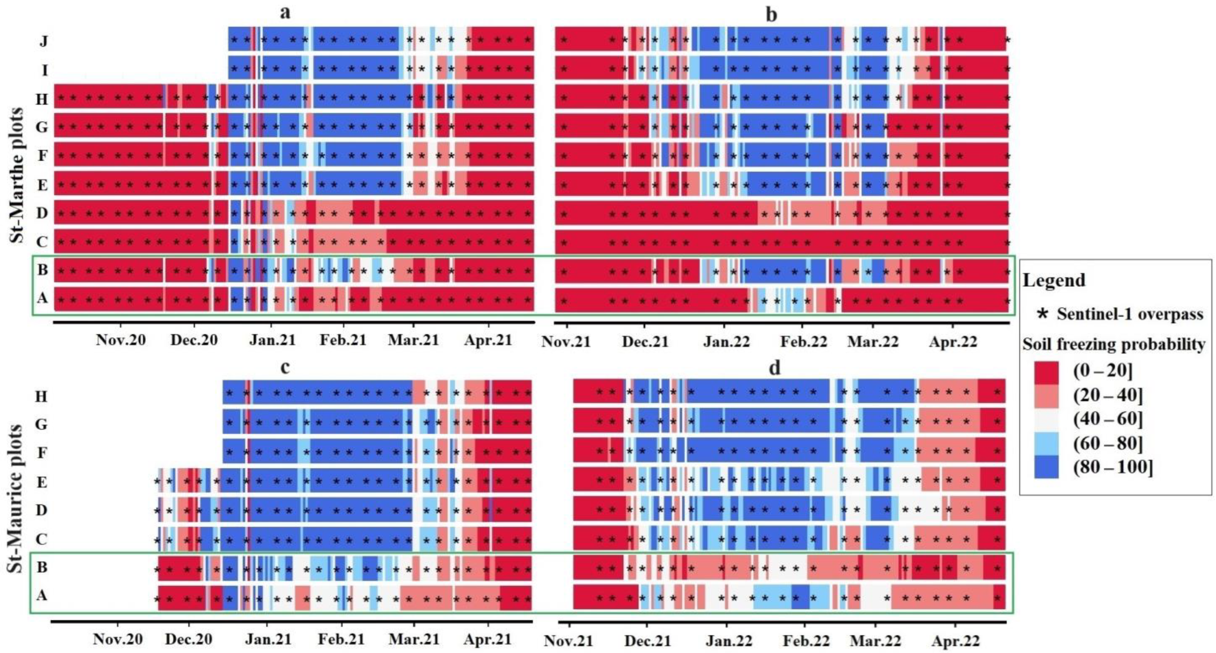
Figure 4.
Comparison of observed 2 cm soil freezing probabilities (dark blue, right Y-axis) with that predicted by the Delta method (top row, in red) and EFTA (bottom row, in red). The S1 corrected VH polarization backscatter signal is also displayed in green. On the left Y-axis, values less than 0 correspond to corrected VH backscatters (green curve), while values greater than 0 correspond to the predicted freezing probability (red curves). (a,b) St-Maurice’s H plot in 2020–21. (c,d) St-Maurice’s H plot in 2021–22. (e,f) St-Marthe’s H plot in 2020–21. (g,h) St-Marthe’s H plot in 2021–22. (i,j) St-Marthe’s I plot in 2020–21. (k,l) St-Marthe’s I plot in 2021–22. The R2 values, derived from the correlation between the soil freezing probability at 2 cm depth and VHDelta (top plots)/and VHEFTA (bottom plots). A dashed line represents the overall trend between VHDelta and the date (top plots) or VHEFTA and the date (bottom plots).

Figure 5.
Local fitted logistic models for observed freezing probability (2 cm) against VHEFTA in St-Marthe (top) and St-Maurice (bottom). (a) St-Marthe’s H agricultural plot. (b) St-Marthe’s I agricultural plot. (c) St-Marthe’s B forest plot. (d) St-Maurice’s F agricultural plot. (e) St-Maurice’s H agricultural plot. (f) St-Maurice’s A forest plot. The top and bottom Pseudo-R2 (Pse-R2) values of each plot are shown for 2020–21 and 2021–22.

Figure 6.
Cross-over interactions of different crop types on the relationship between VHEFTA and the predicted soil freezing probability.
Figure 6.
Cross-over interactions of different crop types on the relationship between VHEFTA and the predicted soil freezing probability.

Figure 7.
Spatial cross-validation results of the Crop-Mixed soil freezing probability model with 28 single folds, showing 14 plots evaluated across two study years: 2020–21 (gray) and 2021–22 (white). The figure displays the Brier score, MAE, and R2 for each fold when individually excluded from calibration and used for validation. The statistical metrics averages for the plots across the study years 2020–21 and 2021–22 exhibited the following respective values: For 2020–21: R2 = 0.55, Brier Score = 0.19, and MAE = 0.18; and for 2021–22: R2 = 0.60, Brier Score = 0.18, and MAE = 0.17.

Figure 8.
Comparison of the soil freezing probability predicted by the Crop-Mixed model vs. observed values. (a) Scatter plot of predicted vs. observed data; (b) frequency histogram showing the accuracy (true positive/negative) and misclassification (false positive/negative) for the different crop types. In the left plot, the red line depicts the best fit for the plotted points, while the gray line illustrates the hypothetical scenario where predicted values perfectly align with observed ones. A smaller gap between these lines signifies the higher model's performance.
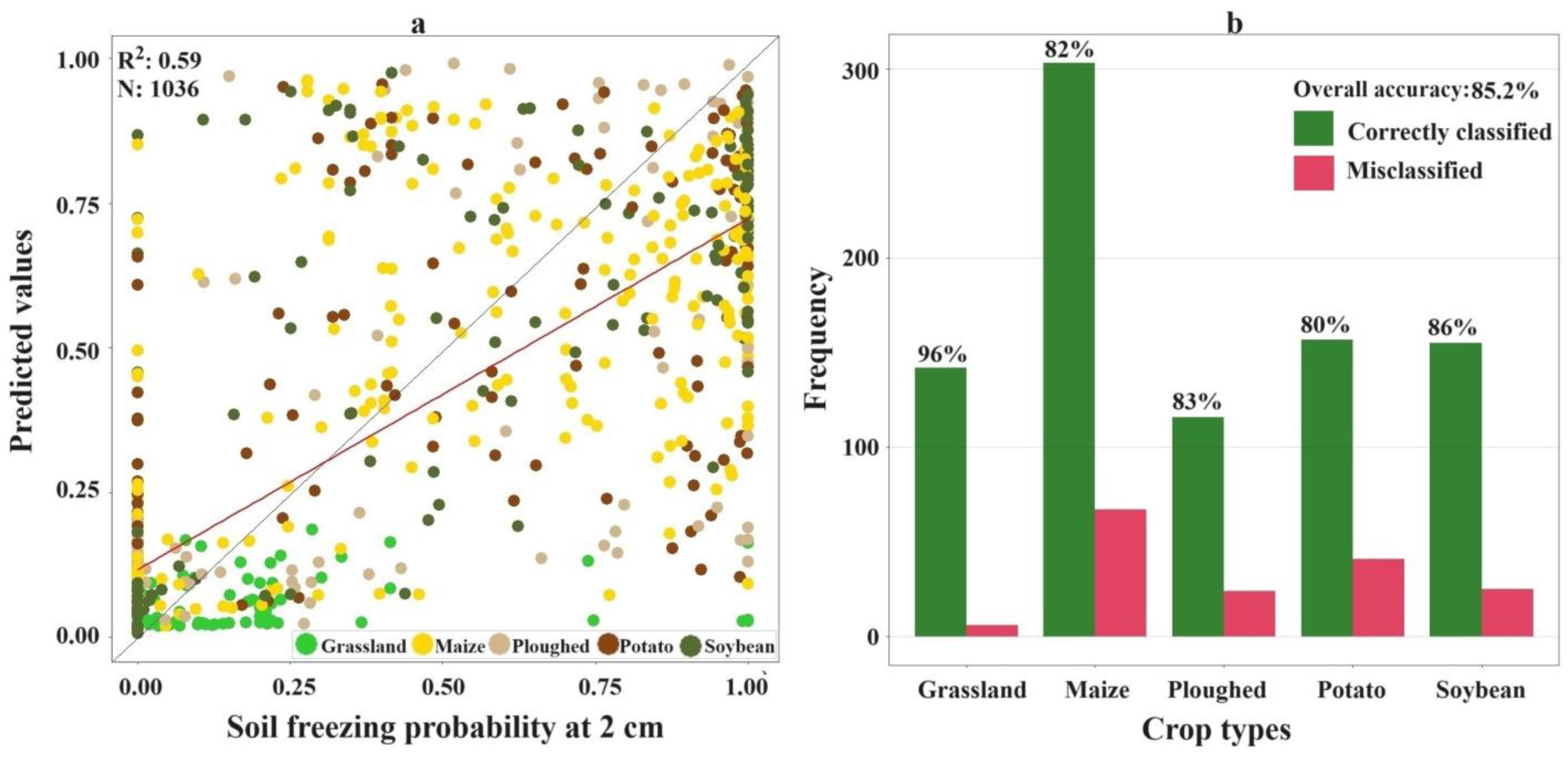

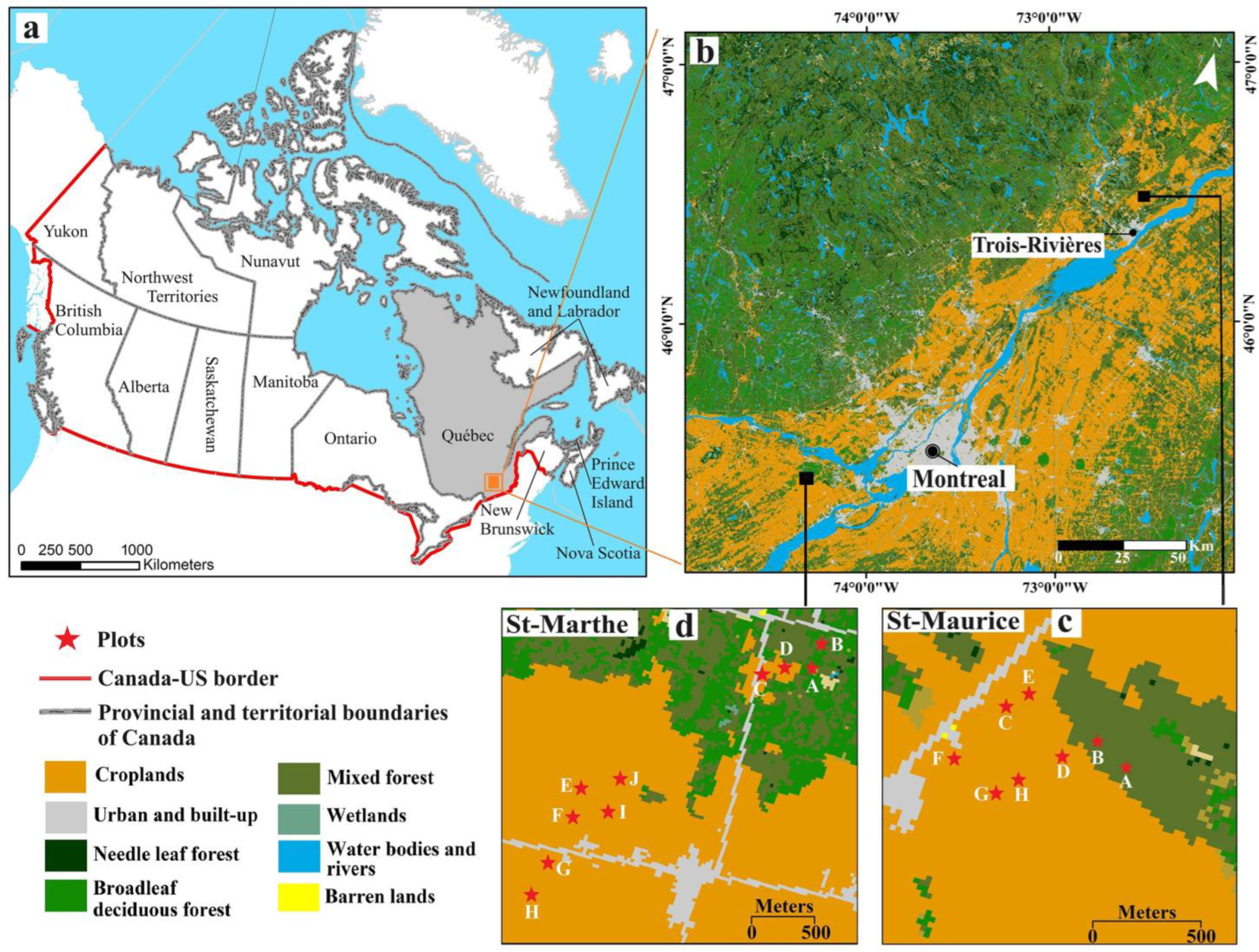
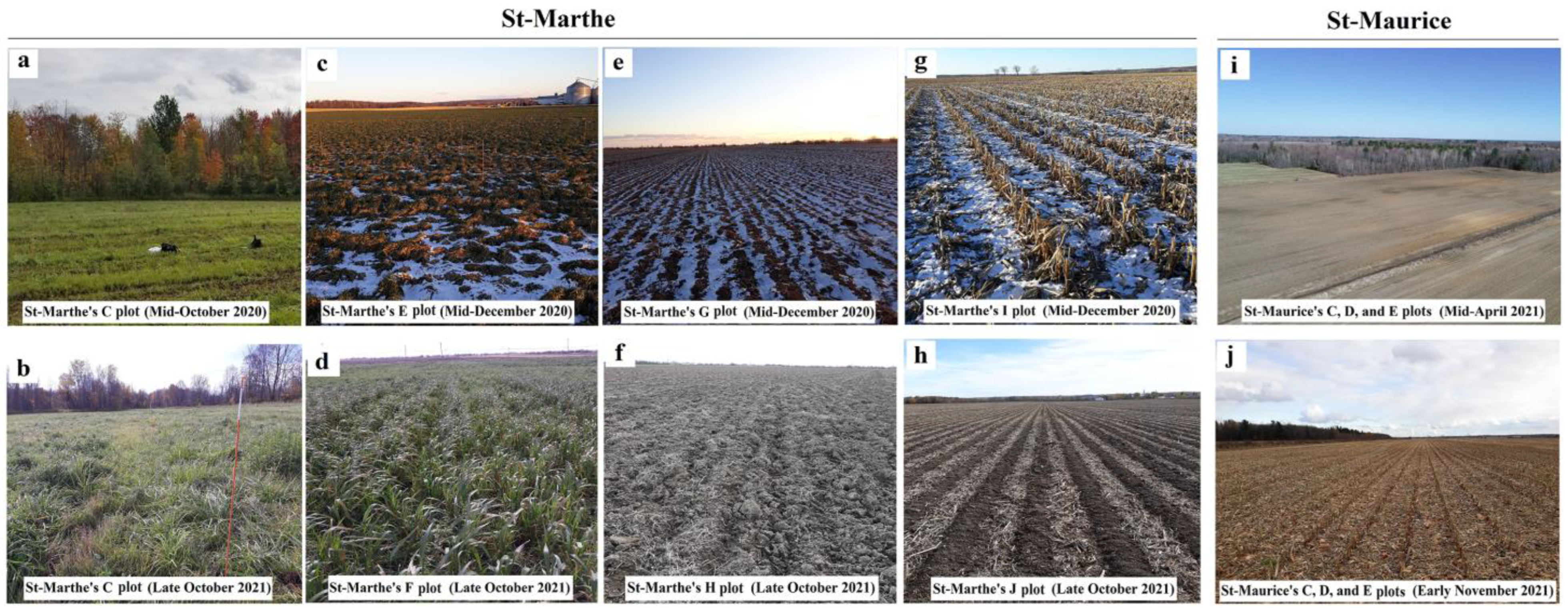
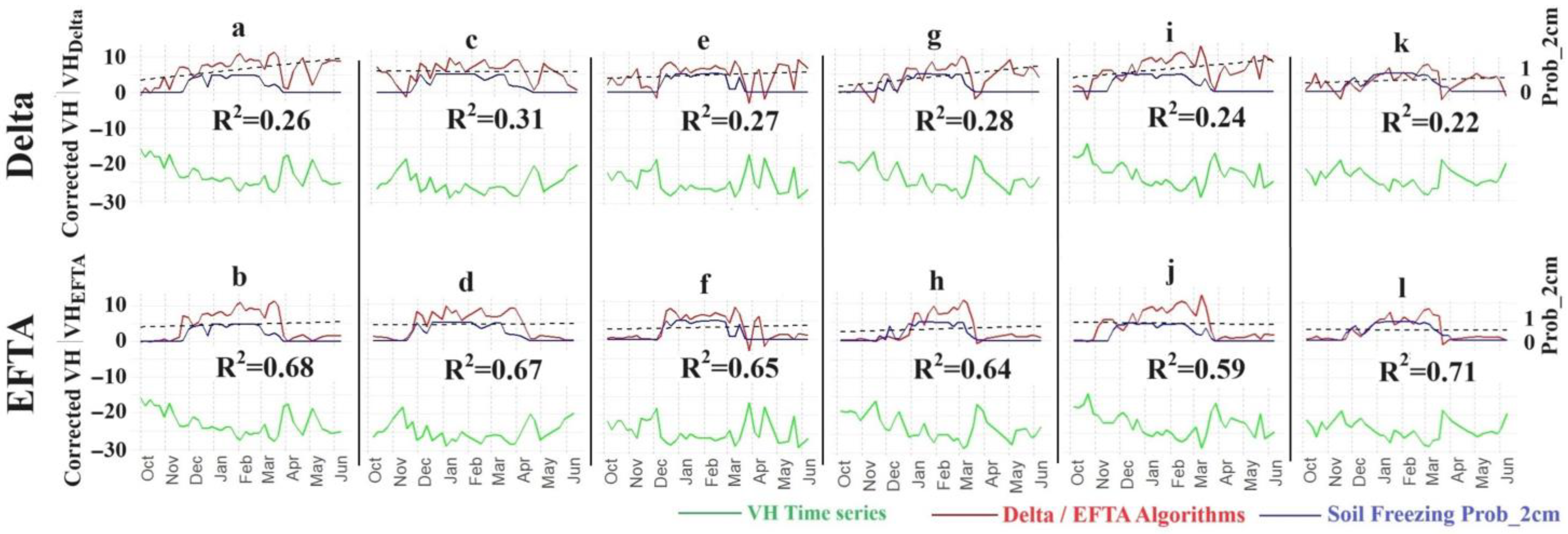
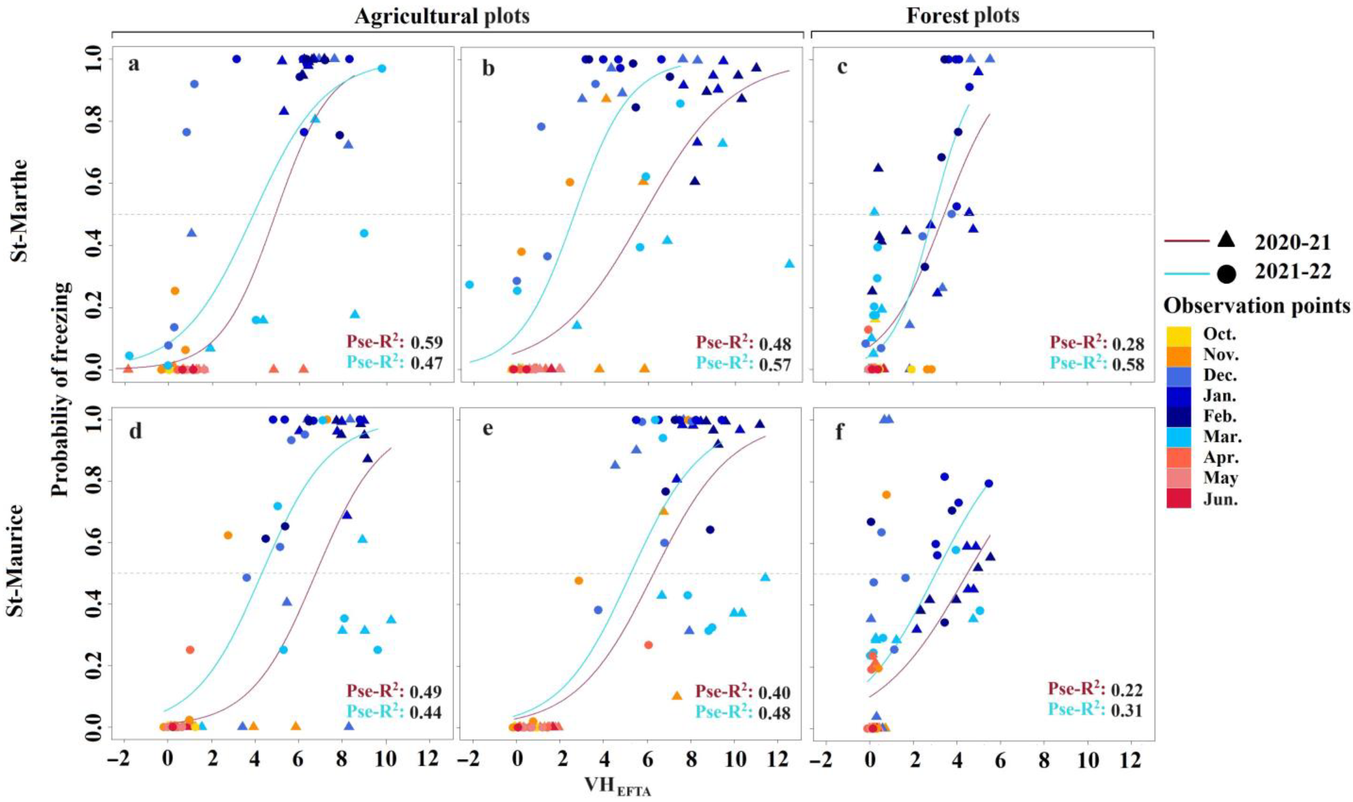
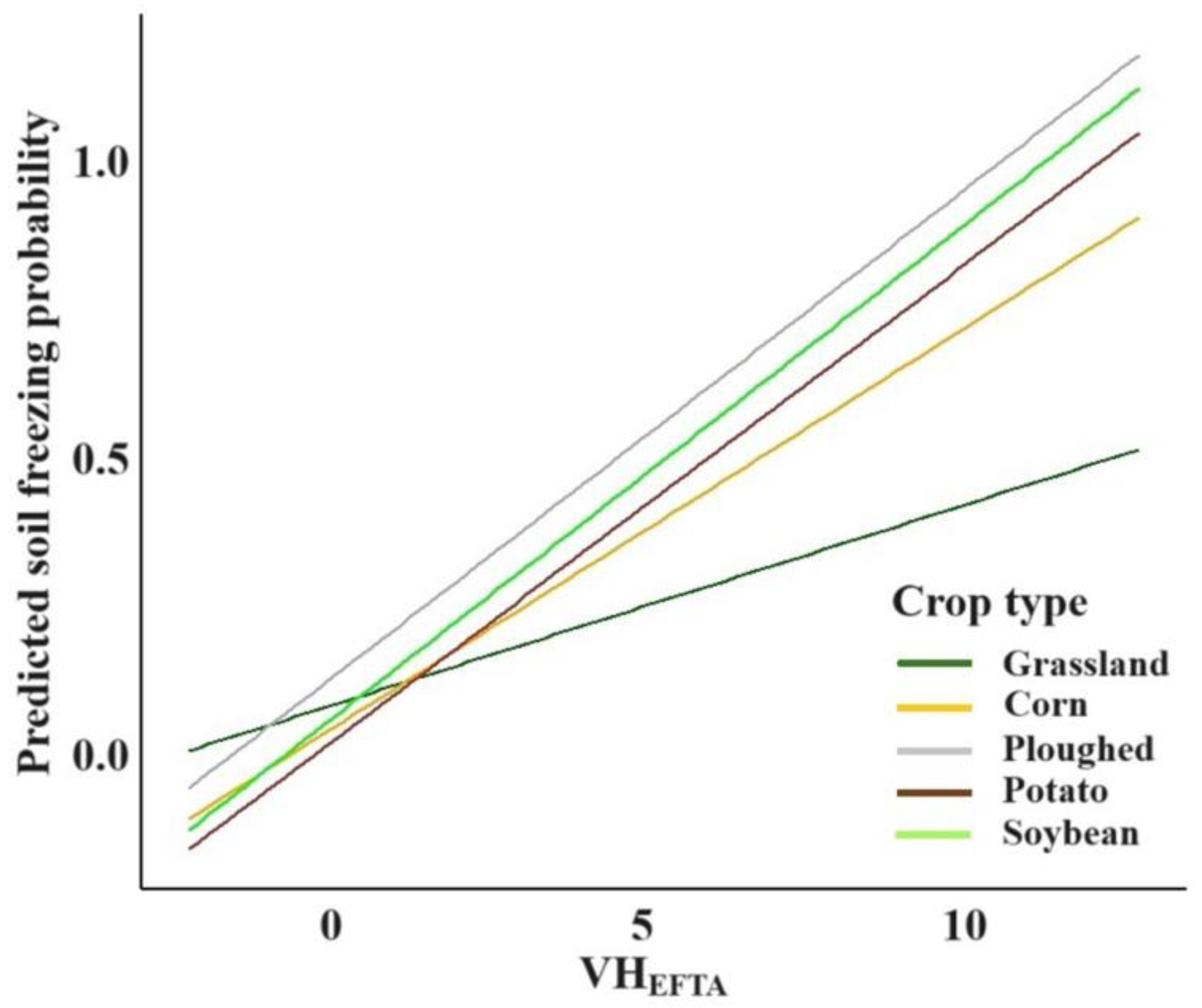
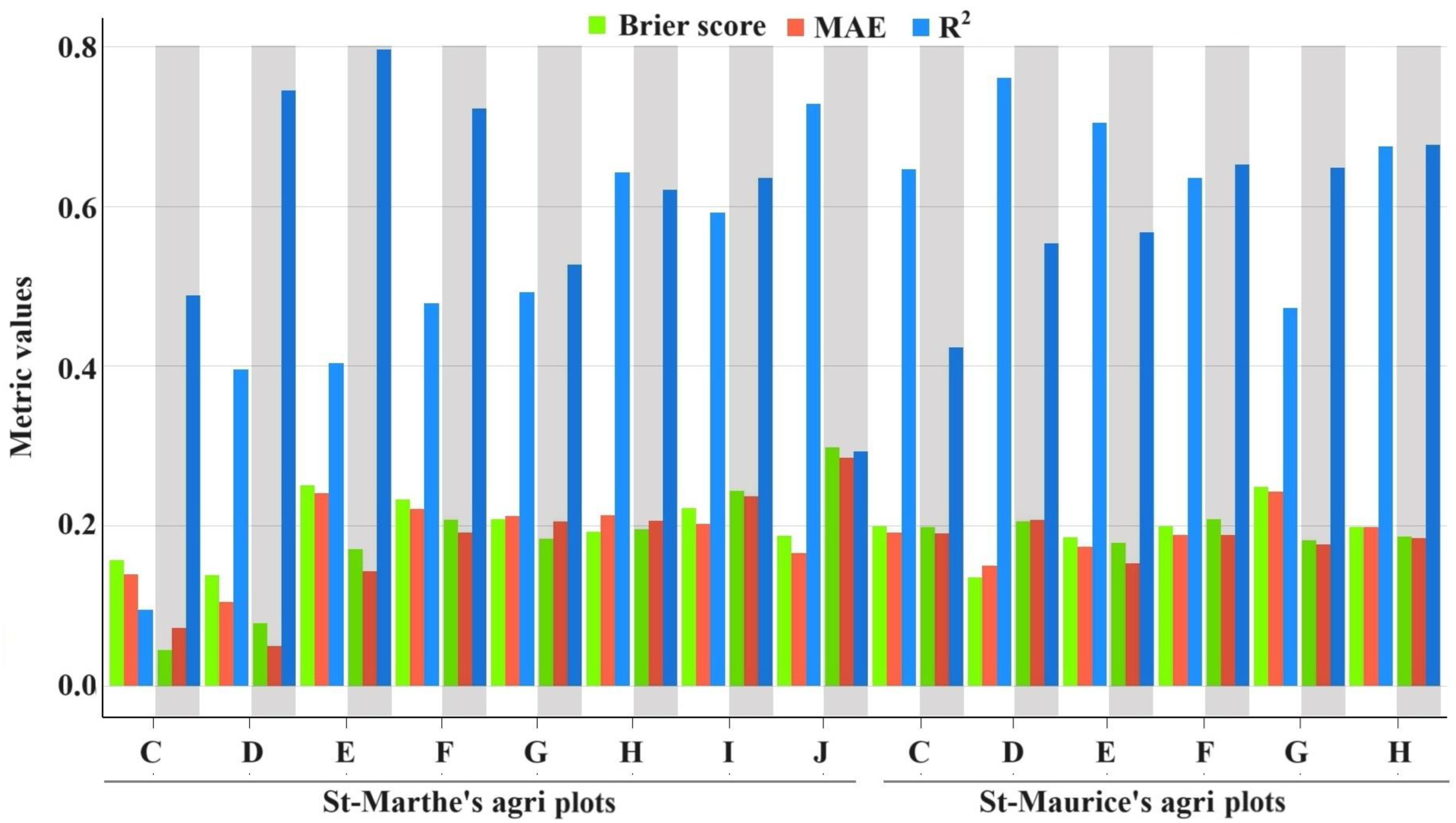
Table 1.
Soil, crop type, and crop residue at each instrumented plot (plot size: 5 m × 5 m).
| Plot | Soil Type | Land Cover/Crop Type | Residues | |||
|---|---|---|---|---|---|---|
| 2020–21 | 2021–22 | 2020–21 | 2021–22 | |||
| St-Maurice | A | Fine sand | Forest | Forest | Forest litter | Forest litter |
| B | Fine sand | Forest | Forest | Forest litter | Forest litter | |
| C | Silty clay | Potato | Corn | Bare field | Corn stalks | |
| D | Silty clay | Potato | Corn | Bare field | Corn stalks | |
| E | Loamy sand | Potato | Corn | Bare field | Corn stalks | |
| F | Silty clay | Corn | Soybean | Corn stalks | Soybean debris | |
| G | Silty clay | Corn | Soybean | Corn stalks | Soybean debris | |
| H | Silty clay | Corn | Soybean | Corn stalks | Soybean debris | |
| St-Marthe | A | Loam | Forest | Forest | Forest litter | Forest litter |
| B | Fine loamy sand | Forest | Forest | Forest litter | Forest litter | |
| C | Fine loamy sand | Grassland | Grassland | Grass | Grass | |
| D | Fine loamy sand | Grassland | Grassland | Grass | Grass | |
| E | Clay | Potato | Corn | Grass | Grass | |
| F | Clay | Potato | Corn | Grass | Grass | |
| G | Clay | Soybean | Ploughed | Soybean debris | Bare field | |
| H | Clay | Soybean | Ploughed | Soybean debris | Bare field | |
| I | Clay | Corn | Ploughed | Corn stalks | Scattered debris | |
| J | Clay | Corn | Ploughed | Corn stalks | Scattered debris | |
Table 2.
Statistical logistic model summary for the EFTA, Delta, and FTI at 2 and 10 cm.
| Algorithms | Soil Depth (cm) | Polarization | Pseudo-R2 | AIC |
|---|---|---|---|---|
| EFTA | 2 | VH | 0.54 | 199 |
| VV | 0.36 | 623 | ||
| 10 | VH | 0.49 | 115 | |
| VV | 0.36 | 194 | ||
| Delta | 2 | VH | 0.32 | 706 |
| VV | 0.22 | 879 | ||
| 10 | VH | 0.27 | 333 | |
| VV | 0.21 | 468 | ||
| FTI | 2 | VH | 0.31 | 714 |
| VV | 0.20 | 918 | ||
| 10 | VH | 0.22 | 445 | |
| VV | 0.16 | 546 |
Table 3.
Comparing probabilistic models of 2 cm depth soil freezing probability based on different site-level predictors. Refer to Section 2.6 for model definitions.
Table 3.
Comparing probabilistic models of 2 cm depth soil freezing probability based on different site-level predictors. Refer to Section 2.6 for model definitions.
| Models | R2 | Pseudo-R2 | AIC | |
|---|---|---|---|---|
| Marginal | Conditional | |||
| 1 | 0.54 | 241 | ||
| 2 | 0.56 | 0.57 | 239 | |
| 3 | 0.55 | 0.58 | 231 | |
| 4 | 0.59 | 0.61 | 232 | |
| 5 | 0.59 | 0.60 | 252 | |
| 6 | 0.59 | 0.60 | 271 | |
Table 4.
Predictor effects for the Crop-Mixed model. σ2 denotes the residual variance, τ00 is the random effect variance at the plot level, and ICC is the intra-class correlation and represents the proportion of total variance attributable to between-group variability, and N Plot denotes the number of agricultural plots used in the analysis. The bold values in the 'p' column indicate statistically significant effects.
| Predictors | Estimates | CI | p |
|---|---|---|---|
| (Intercept) | 0.04 | −0.06–0.14 | 0.441 |
| VHEFTA | 0.04 | 0.02–0.06 | <0.001 |
| Crop type | |||
| Grassland | Reference | ||
| Maize | −0.03 | −0.14–0.08 | 0.593 |
| Ploughed | 0.09 | −0.03–0.21 | 0.142 |
| Potato | −0.05 | −0.17–0.07 | 0.398 |
| Soybean | 0.00 | −0.12–0.12 | 0.989 |
| Crop type and VHFFTA interactions | |||
| VHEFTA: Maize | 0.04 | 0.02–0.07 | 0.001 |
| VHEFTA: Ploughed | 0.06 | 0.03–0.09 | <0.001 |
| VHEFTA: Potato | 0.06 | 0.03–0.08 | <0.001 |
| VHEFTA: Soybean | 0.06 | 0.03–0.09 | <0.001 |
| Random Effects | |||
| σ2 | 0.07 | ||
| τ00 Plot | 0.00 | ||
| ICC | 0.05 | ||
| N Plot | 14 | ||
| Observations | 1036 | ||
| Marginal R2/Conditional R2 | 0.586/0.608 |
Table 5.
Temporal cross-validation of the Crop-Mixed soil freezing model. The R2, MAE, and the Brier score are given for the validation period.
Table 5.
Temporal cross-validation of the Crop-Mixed soil freezing model. The R2, MAE, and the Brier score are given for the validation period.
| State | R2 | MAE | Brier Score |
|---|---|---|---|
| Calibration 2020–21, validation 2021–22 | 0.60 | 0.18 | 0.19 |
| Calibration 2021–22, validation 2020–21 | 0.56 | 0.18 | 0.17 |
Disclaimer/Publisher’s Note: The statements, opinions and data contained in all publications are solely those of the individual author(s) and contributor(s) and not of MDPI and/or the editor(s). MDPI and/or the editor(s) disclaim responsibility for any injury to people or property resulting from any ideas, methods, instructions or products referred to in the content. |
© 2024 by the authors. Licensee MDPI, Basel, Switzerland. This article is an open access article distributed under the terms and conditions of the Creative Commons Attribution (CC BY) license (https://creativecommons.org/licenses/by/4.0/).
Share and Cite
MDPI and ACS Style
Taghipourjavi, S.; Kinnard, C.; Roy, A. Sentinel-1-Based Soil Freeze–Thaw Detection in Agro-Forested Areas: A Case Study in Southern Québec, Canada. Remote Sens. 2024, 16, 1294. https://doi.org/10.3390/rs16071294
AMA Style
Taghipourjavi S, Kinnard C, Roy A. Sentinel-1-Based Soil Freeze–Thaw Detection in Agro-Forested Areas: A Case Study in Southern Québec, Canada. Remote Sensing. 2024; 16(7):1294. https://doi.org/10.3390/rs16071294
Chicago/Turabian StyleTaghipourjavi, Shahabeddin, Christophe Kinnard, and Alexandre Roy. 2024. "Sentinel-1-Based Soil Freeze–Thaw Detection in Agro-Forested Areas: A Case Study in Southern Québec, Canada" Remote Sensing 16, no. 7: 1294. https://doi.org/10.3390/rs16071294
Note that from the first issue of 2016, this journal uses article numbers instead of page numbers. See further details here.