Technical Note

SSEBop Evapotranspiration Estimates Using Synthetically Derived Landsat Data from the Continuous Change Detection and Classification Algorithm

by
Mikael P. Hiestand
1,2,*,
Heather J. Tollerud
1,
Chris Funk
2,
Gabriel B. Senay
3,
Kate C. Fickas
1,2 and
MacKenzie O. Friedrichs
4
1
U.S. Geological Survey (USGS), Earth Resources Observation and Science (EROS) Center, Sioux Falls, SD 57198, USA
2
Climate Hazards Center, University of California, Santa Barbara, CA 93106, USA
3
U.S. Geological Survey (USGS), Earth Resources Observation and Science (EROS) Center, North Central Climate Adaptation Science Center, Fort Collins, CO 80523, USA
4
KBR, Contractor to the USGS, EROS Center, Sioux Falls, SD 57198, USA
*
Author to whom correspondence should be addressed.
Remote Sens. 2024, 16(7), 1297; https://doi.org/10.3390/rs16071297
Submission received: 9 March 2024 / Accepted: 1 April 2024 / Published: 6 April 2024

Abstract

:
The operational Simplified Surface Energy Balance (SSEBop) model has been utilized to generate gridded evapotranspiration data from Landsat images. These estimates are primarily driven by two sources of information: reference evapotranspiration and Landsat land surface temperature (LST) values. Hence, SSEBop is limited by the availability of Landsat data. Here, in this proof-of-concept paper, we utilize the Continuous Change Detection and Classification (CCDC) algorithm to generate synthetic Landsat data, which are then used as input for SSEBop to generate evapotranspiration estimates for six target areas in the continental United States, representing forests, shrublands, and irrigated agriculture. These synthetic land cover data are then used to generate the LST data required for SSEBop evapotranspiration estimates. The synthetic LST, evaporative fractions, and evapotranspiration data from CCDC closely mirror the phenological cycles in the observed Landsat data. Across the six sites, the median correlation in seasonal LST was 0.79, and the median correlation in seasonal evapotranspiration was 0.8. The median root mean squared error (RMSE) values were 2.82 °C for LST and 0.50 mm/day for actual evapotranspiration. CCDC predictions typically underestimate the average evapotranspiration by less than 1 mm/day. The average performance of the CCDC evaporative fractions, and corresponding evapotranspiration estimates, were much better than the initial LST estimates and, therefore, promising. Future work could include bias correction to improve CCDC’s ability to accurately reproduce synthetic Landsat data during the summer, allowing for more accurate evapotranspiration estimates, and determining the ability of SSEBop to predict regional evapotranspiration at seasonal timescales based on projected land cover change from CCDC.

1. Introduction

Understanding spatial and temporal patterns in actual evapotranspiration (ETa) through remotely sensed data products is of increasing importance for a variety of environmental applications in the continental United States. First and foremost, satellite-derived ETa data are an integral part of drought monitoring [1,2,3]. Furthermore, utilizing remotely sensed ETa data in agricultural regions can help inform stakeholders managing evaporative water loss, allowing them to optimize irrigation [4]. Gridded ETa data have been used to monitor the hydrological balance in relation to forest fires [5]. Additionally, gridded ETa datasets have been used to produce an evapotranspiration climatology for the state of Indiana for analyzing the regional water budget and drought’s effects on cereal production [6].
To meet these increasing needs for spatial evapotranspiration data, a variety of gridded evapotranspiration data products have been developed to utilize remote sensing data from a variety of satellite platforms. These satellite-derived evapotranspiration models typically use thermal data from satellites, such as GOES, as is the case for the Atmosphere–Land Exchange Inverse (ALEXI) model [7], or Landsat for the operational Simplified Surface Energy Balance (SSEBop) model [8]. Recently, ALEXI and SSEBop have been aggregated together with several other remote-sensing-based evapotranspiration models to produce the OpenET project, which provides evapotranspiration data for stakeholders in the western United States [9]. Additionally, NASA has recently deployed ECOSTRESS onboard the International Space Station to capture evapotranspiration data at 70 m spatial resolution with a 1- to 5-day repeat time [10]. Landsat provides higher spatial resolution at 30 m but is still limited by its 16-day repeat time.
Despite the clear need for quality ETa estimates, hydrological forecasters typically rely on reference evapotranspiration (ET0) when making predictions. Several different approaches have been successfully utilized to forecast ET0 for agricultural applications, including probabilistic forecasting [11], numerical weather prediction [12,13], wavelet regression models [14], and machine learning [15,16]. Additionally, ET0 forecasts can lead to improved drought forecasts [17]. However, ET0 is typically modeled on large spatial scales [18] that may not be useful for individual stakeholders. Furthermore, ET0 measures potential atmospheric water demand, which varies greatly from ETa in water-stressed environments. Hence, more localized forecasts of water losses through ETa are needed. Here, we take the first step necessary for combining modeled ET0 with Landsat data to provide ETa estimates at 30 m spatial resolution and sub-seasonal timescales.
This proof-of-concept paper uses synthetic Normalized Difference Vegetation Index (NDVI) and thermal infrared Landsat data produced with the Continuous Change Detection and Classification (CCDC) algorithm [19] to generate ETa estimates at a spatial resolution of 30 m on daily timestamps using the SSEBop algorithm. On a per-pixel basis, we use CCDC’s harmonic fitting algorithm to calculate synthetic surface reflectance values and brightness temperatures corresponding to Landsat overpasses at six target areas in the western United States. These synthetic surface reflectance values and brightness temperatures are then used to generate synthetic NDVI and land surface temperature (LST) data, which are input into SSEBop to derive synthetic ETa estimates. The CCDC-derived ETa estimates are validated against ETa estimates from Landsat data in six target areas, representing croplands, forest, and shrublands in the western United States. The work presented in this paper paves the way for using synthetic Landsat data to generate ETa estimates between Landsat overpasses, thus allowing for daily ETa estimates from SSEBop and addressing the limited temporal resolution offered by Landsat. Now that this paper validates the ability of CCDC to generate accurate synthetic ETa estimates through SSEBop, future work can focus on generating synthetic ETa estimates between Landsat overflies, with the goal of extending CCDC into the future to generate sub-seasonal ETa forecasts.

2. Materials and Methods

2.1. Calculation of ETa Data from SSEBop

For this study, we used the most recent edition of SSEBop, which uses the Forcing and Normalizing Operation (FANO) approach [20]. SSEBop was initially outlined by Senay et al. [8] and uses the Surface Energy Balance Algorithm for Land [21] as its theoretical basis to derive ETa by comparing the difference between hot and cold pixels in remotely sensed surface temperatures [22]. The current FANO approach allows for the accurate derivation of cold boundary (wet bulb) LST from Landsat data utilizing localized LST and NDVI values [20]. From there, the evaporative fraction (ETf) was calculated using Equation (1):
ETf = 1 − γs (TsTc)
where Ts is the observed satellite LST, Tc is the wet bulb surface temperature, and γs is the surface psychrometric constant derived from ERA 5, or the fifth-generation ECMWF atmospheric reanalysis of the global climate [23]. The ETf is then multiplied by the alfalfa reference evapotranspiration (ETr), as determined by gridMet [24], to obtain the actual evapotranspiration (ETa; Equation (2)):
ETa = ETf × ETr
The main advantage to SSEBop is that as a two-parameter model, it is easy to deploy and less prone to uncertainties that could arise from a more complex model with additional parameters. Additionally, an advantage of using this surface temperature gradient approach between hot and cold pixels in satellite images is that it does not require absolutely accurate LST, but rather depends on the magnitude of the difference between hot and cold pixels [22], as illustrated in Equation (1). Conversely, as a simple model, SSEBop does not generate other components of the energy balance, such as the sensible and ground heat fluxes. An additional drawback to SSEBop is the limited temporal resolution resulting from Landsat’s 8- to 16-day repeat time and cloud cover [25]. Nonetheless, SSEBop has been shown to provide accurate ETa estimates for irrigated crops in Brazil [26,27] and Egypt [28], in addition to the continental United States [20,29,30].
Here, SSEBop was run on Landsat Collection 2 Level-2 [31], which corresponds to six target areas in the western United States (discussed below). All Landsat scenes from 2019 for each of the six target areas were utilized to generate ETa estimates for comparison to the synthetic ETa estimates produced in this study. Landsat scenes with greater than 70 percent cloud clover, as identified by the Landsat Level-2 QA pixel band, or that only contained part of a target area, were excluded from this study. Additionally, this same cloud mask was used to remove all corresponding cloud-contaminated pixels from the synthetic datasets to avoid biasing the comparisons. These scenes were selected to provide a good representation of water-limited areas in the western United States, where SSEBop is widely used, while also providing a small enough sample size so that individual scenes could be visualized and analyzed in detail.

2.2. Landsat and Synthetic CCDC Data

This study utilized Analysis Ready Data (ARD) from Landsat 8 [32]. Landsat ARD incorporates several preprocessing techniques that standardize data across the Landsat archive and allow for the scientific analysis of Landsat data. First, the ARD normalizes top-of-atmosphere reflectance and brightness temperature values with respect to the cosine of the zenith angle [33]. Additionally, atmospheric corrections for the ARD from Landsat 8 are implemented using the Landsat Surface Reflectance Code [34] and contain a QA band that allows for the filtering of cloud-contaminated pixels [33]. Further, Landsat ARD data follow the Committee on Earth Observation Satellites ARD surface reflectance Product Family Specifications [35].
The initial input for the synthetic ETa was land cover data from the Land Change Monitoring Assessment and Projection (LCMAP) project, which were derived from the CCDC algorithm. LCMAP utilizes ARD [36] after cloud-contaminated pixels have been removed using the Fmask algorithm [37,38]. To generate LCMAP data, CCDC fits a harmonic model to each individual band in the Landsat ARD to generate per-pixel estimates [19]. The CCDC harmonic model (Equation (3)) can then be used to generate synthetic Landsat images and predict surface reflectance for any given date [39].
Here, the harmonic models produced during the LCMAP Collection 1.2 run of CCDC were used to generate synthetic Landsat data for six target areas (discussed below) on dates corresponding to every Landsat flyover for each target area during 2019. On a per-pixel basis, synthetic surface reflectance values and brightness temperatures were calculated from CCDC using the full harmonic model shown in Equation (3) [39]:
ρ ^ i , x f u l l = a 0 , i + a 1 , i c o s 2 π T x + b 1 , i s i n 2 π T x + c 1 , i x + a 2 , i c o s 4 π T x + b 2 , i s i n 4 π T x + a 3 , i c o s 6 π T x + b 3 , i s i n 6 π T x
where,
  • x: Julian date
  • i: the ith Landsat band (i = 1, 2, 3, 4, 5, and 7)
  • T: number of days per year (T = 365.25)
  • a0,i: coefficient for overall value for the ith Landsat band
  • a1,i, b1,i: coefficients for intra-annual change for the ith Landsat band
  • c1,i: coefficient for inter-annual change (slope) for the ith Landsat band
  • a2,i, b2,i: coefficients for intra-annual bimodal change for the ith Landsat band
  • a3,i, b3,i: coefficients for intra-annual trimodal change for the ith Landsat band
  • ρ ^ (i,x)full: predicted value for the ith Landsat band at Julian date x
Equation (3) was used to generate synthetic Landsat data in the thermal infrared, near-infrared (NIR), green, and red bands, which are required for running SSEBop. These pixel-level data were then assembled into raster stacks representing a time series of synthetic data that correspond to the days of Landsat overpasses at each target area. The thermal band was used to produce synthetic brightness temperatures, while the red and NIR bands were used to produce NDVI: (NIR − Red)/(NIR + Red), and the green and NIR bands were used to produce the Normalized Difference Water Index (NDWI): (Green − NIR)/(Green + NIR). A water mask was generated from the NDWI data for pixels with NDWI values greater than 0.1. These synthetic datasets were then uploaded into Google Earth Engine for integration into SSEBop model version 0.2.6 within Google Earth Engine [30]. Brightness temperatures were converted to LST [22] and Tc using the FANO process [20]. SSEBop was run on the resulting synthetic LST rasters with the NDWI and water masks used to identify and model open water and wet areas to prevent those pixels from being included in the Tc parameterization. Finally, the pixels of synthetic data that corresponded to cloud-contaminated pixels in the Landsat data were masked out to allow for a direct one-to-one comparison between the two datasets.

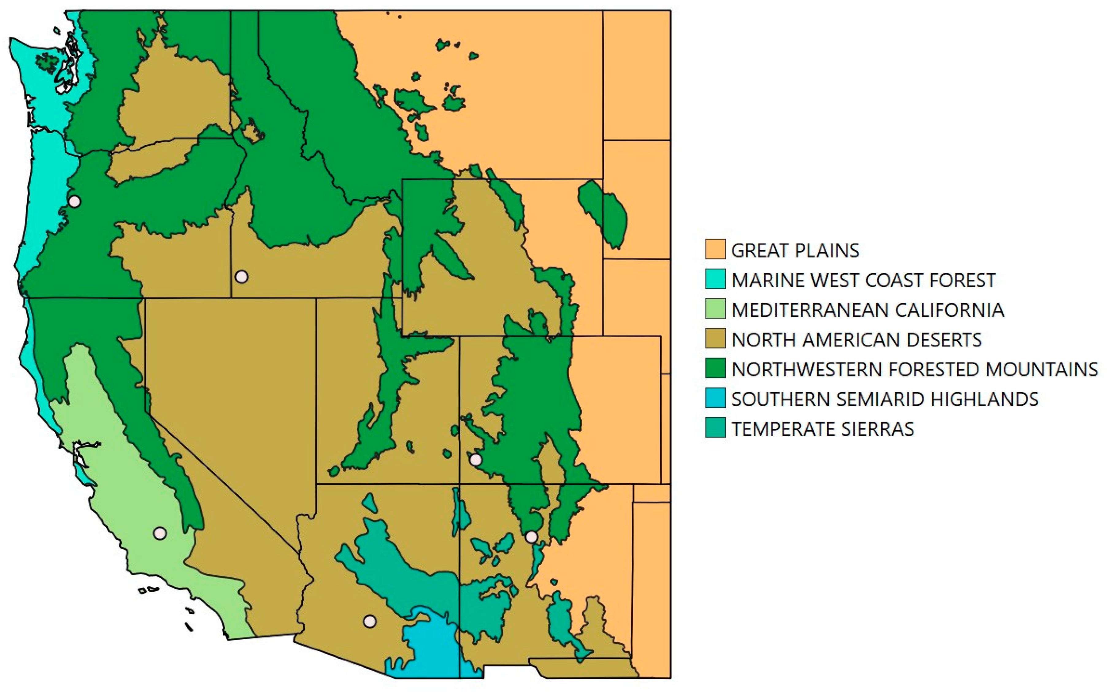
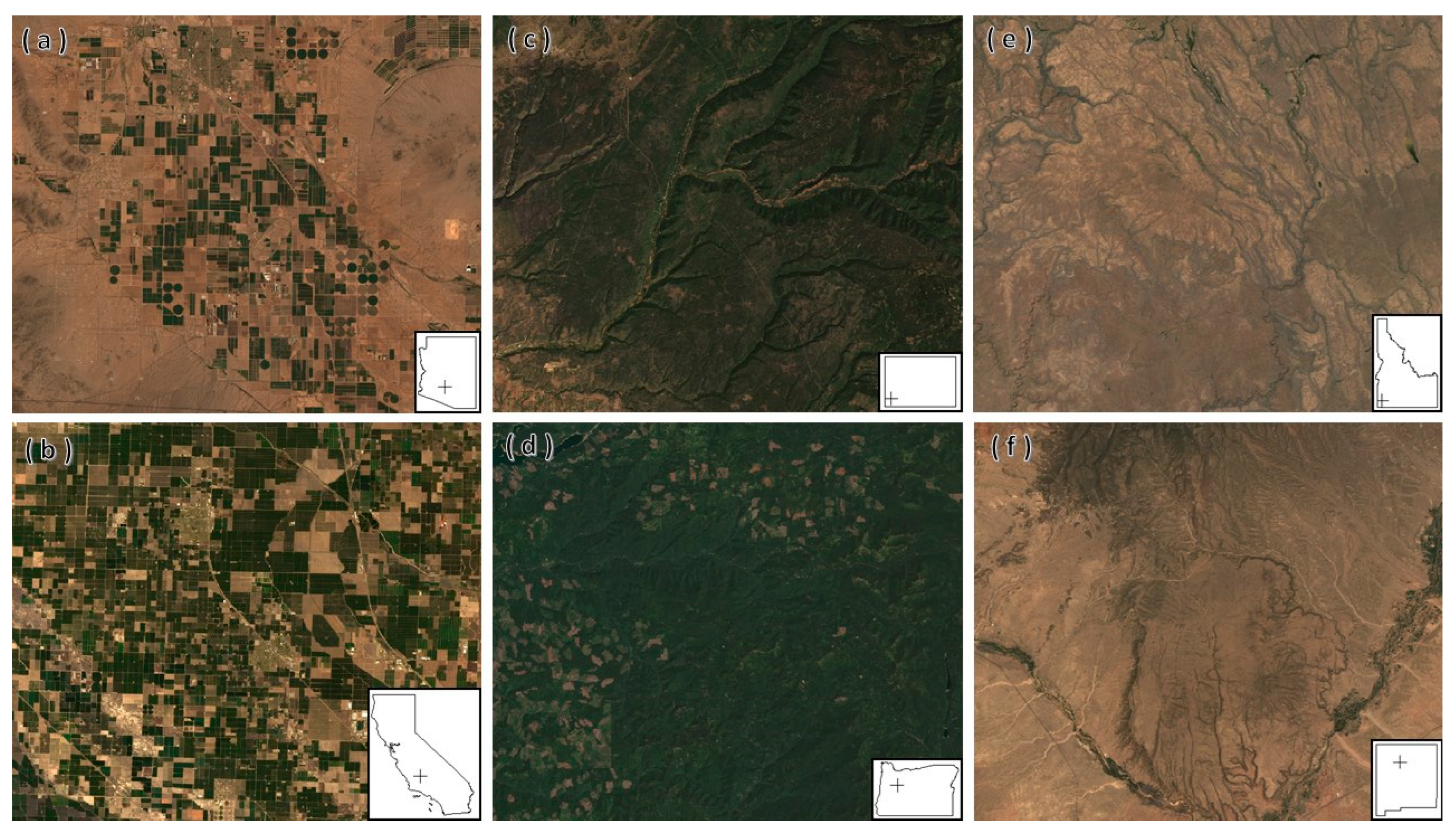
2.3. Site Selection and Study Areas

To determine how well synthetic data can be used to produce ETa estimates with SSEBop, we selected six target areas in the western United States that represent economically important land cover types of forests, irrigated croplands, and shrubland. The locations of the six target areas and their associated ecoregions [40] are shown in Figure 1, and the target areas themselves are depicted in Figure 2. For each target area, a 30-by-30 km grid of 30 m synthetic data was generated for the thermal infrared, red, green, and NIR bands required to generate the input rasters for SSEBop. For this proof-of-concept paper, the small size of the target areas limited variations in land cover, allowing for a more focused evaluation of Landsat and synthetic ETa estimates. Additionally, the target areas were intentionally kept small to limit the computational resources needed for developing multilayer synthetic datasets and to facilitate data transfers to Google Earth Engine for SSEBop. For each target site, synthetic reflectance and thermal data were generated for every day in 2019 that corresponded to Landsat flyover with less than 70% cloud cover. To avoid uncertainties in the final year of the time series, the year 2019 was selected, because LCMAP Collection 1.2 extends through 2020.
Individual target areas were selected in areas where SSEBop has been shown to perform well and validated against flux tower data [8,30], including the Central Valley of California and the Colorado River Basin [29]. The land cover type in each target area was determined using data from the USGS’s LCMAP database [41]. In the case of agricultural areas, the United States Department of Agriculture’s (USDA) 2019 Crop Scape data layer [42] was utilized to identify the crops growing in each target area. The first target area is an almond plantation in the Central Valley of California (Kern County), just northwest of Bakersville. In addition to almonds, small amounts of grapes, alfalfa, pistachios, peanuts, and corn also fall within this Californian target area. The second target area is an agricultural region in the lower Colorado River Basin, south of Phoenix, Arizona (Pinal County), and it is composed mainly of alfalfa, cotton, and corn, surrounded by desert shrubland. The third target area is in the upper Colorado River basin in southwestern Colorado (Dolores County), and it consists almost entirely of evergreen forests. The fourth target area is northeast of Eugene, Oregon (Linn County), and it consists almost entirely of evergreen forests. The fifth target area consists mostly of shrubland and a small amount of evergreen forest in the Santa Anna Pueblo Forest, just north of Albuquerque, New Mexico (Sandoval County), and it encompasses a small stretch of the Rio Grande River. The sixth and final target area is in the southwestern corner of Idaho (Owyhee County) and consists entirely of shrublands. The county-wide average temperatures and total precipitation for 2019 at each target area are presented in Table 1.

3. Results

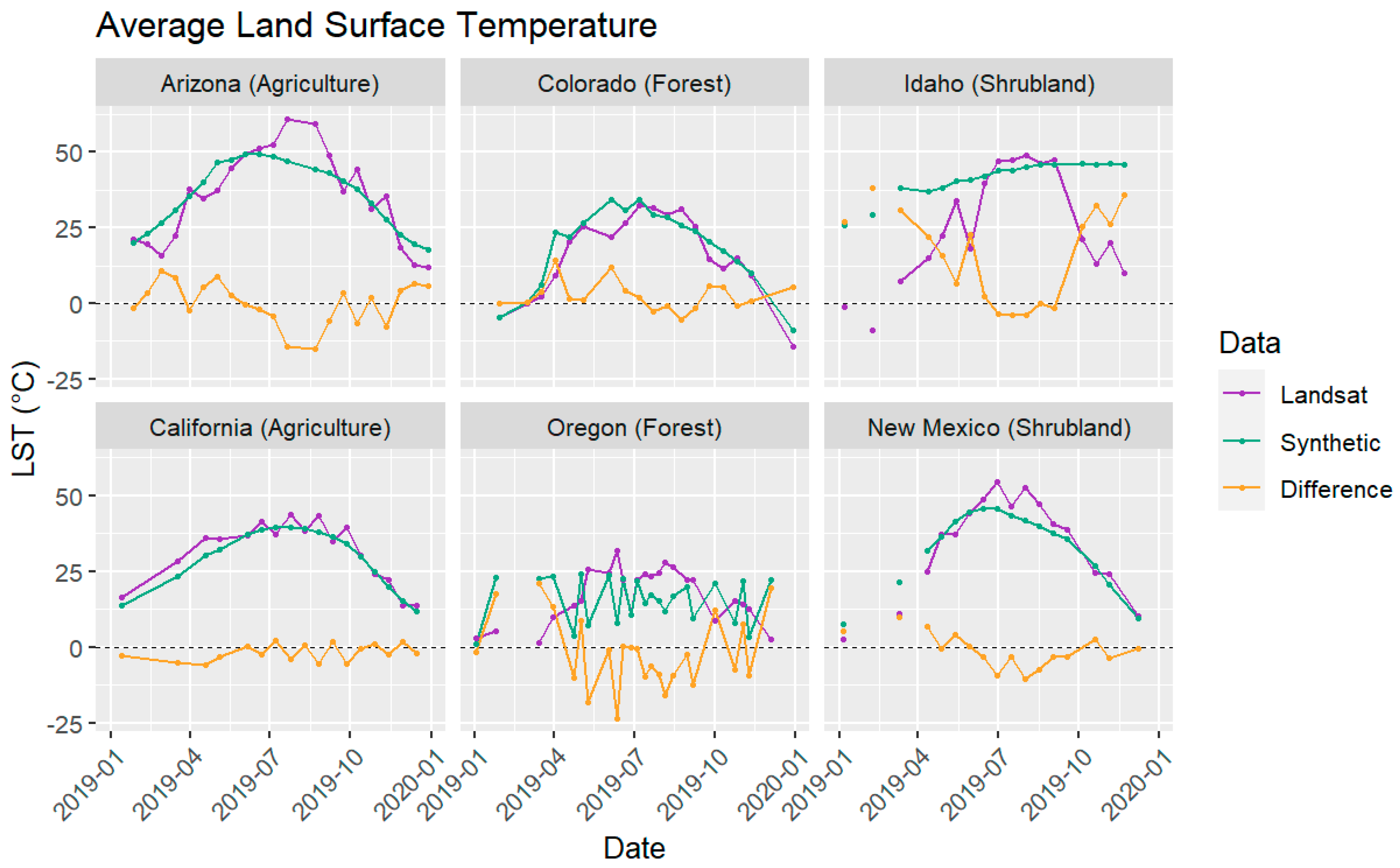
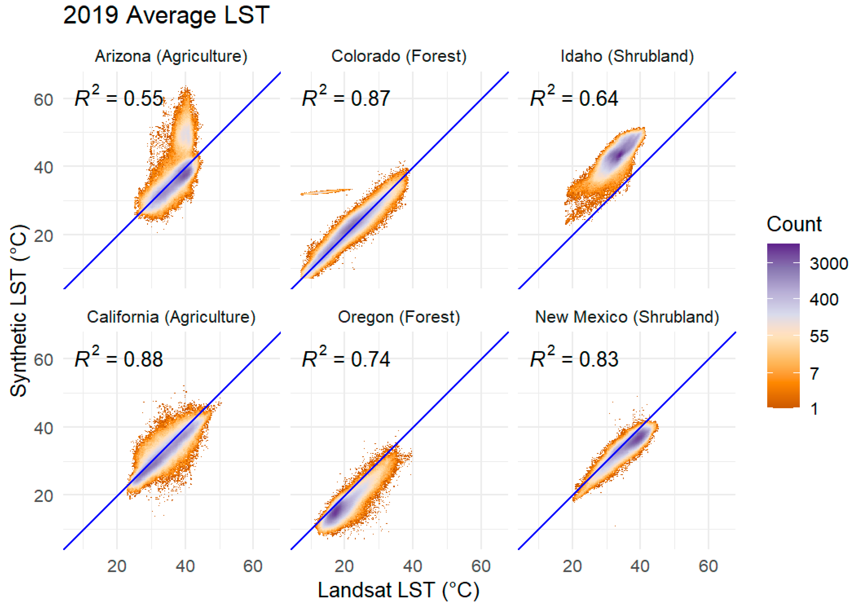
3.1. Land Surface Temperature

The first check on the synthetic data was an examination of how well they reproduce LST in comparison to observed LST from Landsat. Target-area-wide spatial averages of synthetic LST and observed LST are shown in Figure 3. The synthetic LSTs followed the general annual cycle in surface temperatures observed for 2019 for the four southernmost target areas in Arizona, California, Colorado, and New Mexico. However, the synthetic LSTs underestimated the average maximum summer temperatures for each target area and overestimated the average winter and spring surface temperatures in the Arizona and Colorado target areas. This general estimation of summertime LST stems from the lasso regression algorithm [43] used by CCDC that smooths under the summertime peaks in the observed Landsat surface brightness temperatures used to generate the synthetic LST estimates. Then, as expected, the synthetic LST did not capture temperature variations in relation to weather. For the Idaho and Oregon target areas, the synthetic LST did not fully capture the seasonal cycles observed in the Landsat data; however, this did not negatively affect the ETf and ETa estimates (discussed below).
Per-pixel comparisons between the annual averages for the six target areas (Figure 4) and their differences between their overall means (Table 2) showed that synthetic LST generally underestimated the observed LST from Landsat data. This underestimate in the synthetic LST was particularly evident in the California, New Mexico, and Oregon target areas. The Arizona target area showed two clear signals for each of its land cover types. The cropland in Arizona followed the typical trend of the synthetic LST data underestimating the observed LST, whereas it overestimated LST in the surrounding desert regions. Generally, for the Colorado target area, the synthetic LST closely matched the observed LST. However, on the eastern edge of the forested Colorado target area are two regions of dense forest, where the synthetic LST overestimated the observed LST, resulting in the cluster of outliers shown in Figure 4. Idaho stood out as being the only target area where the synthetic LST overestimated the observed LST. However, because ETf estimation depends on the difference between Ts and Tc (Equation (1)) and that exact LST, CCDC was still able to produce reliable ETf estimates (discussed below). The root mean squared errors (RMSE) between the CCDC and Landsat 2019 average LSTs are shown in Table 3.

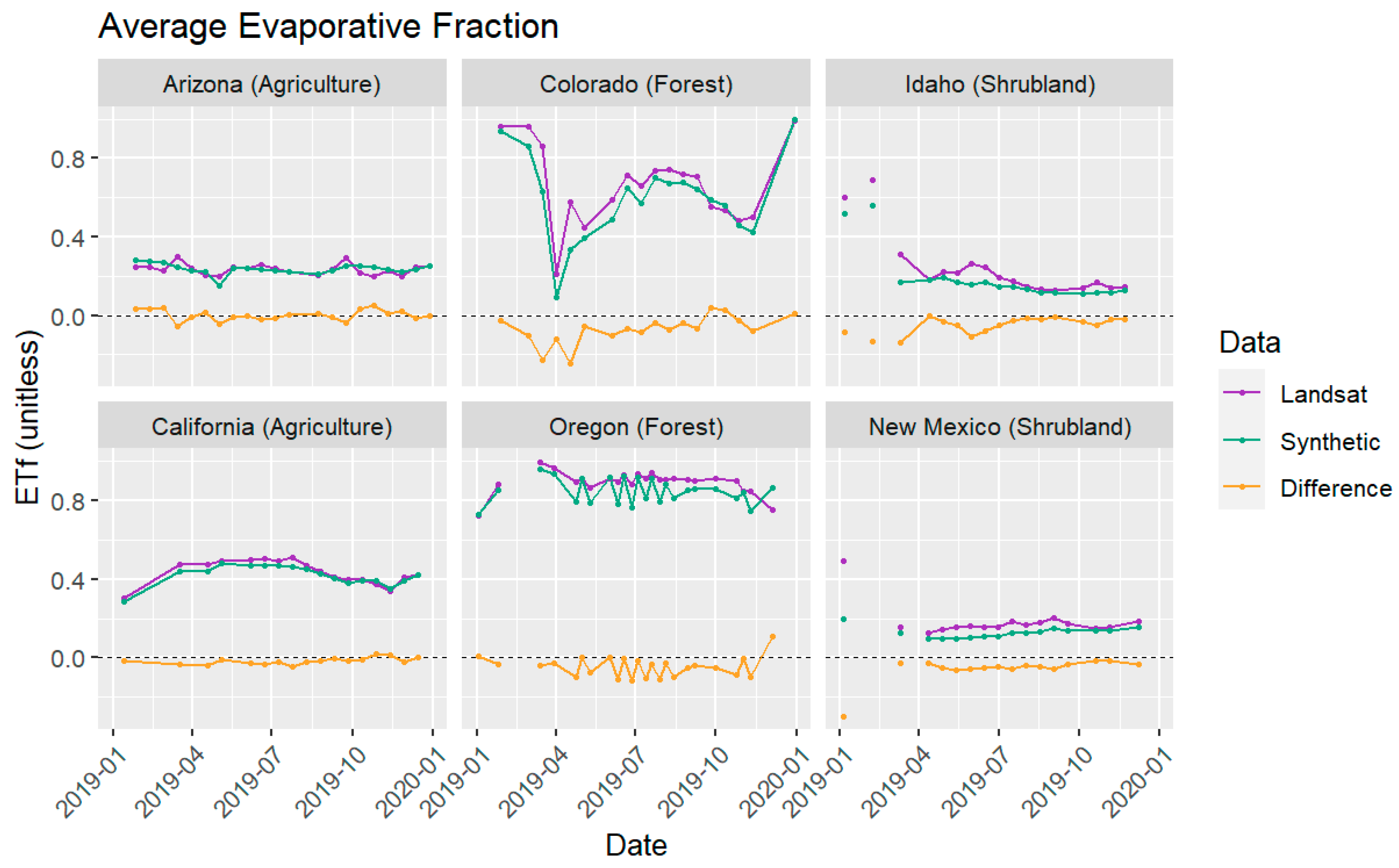
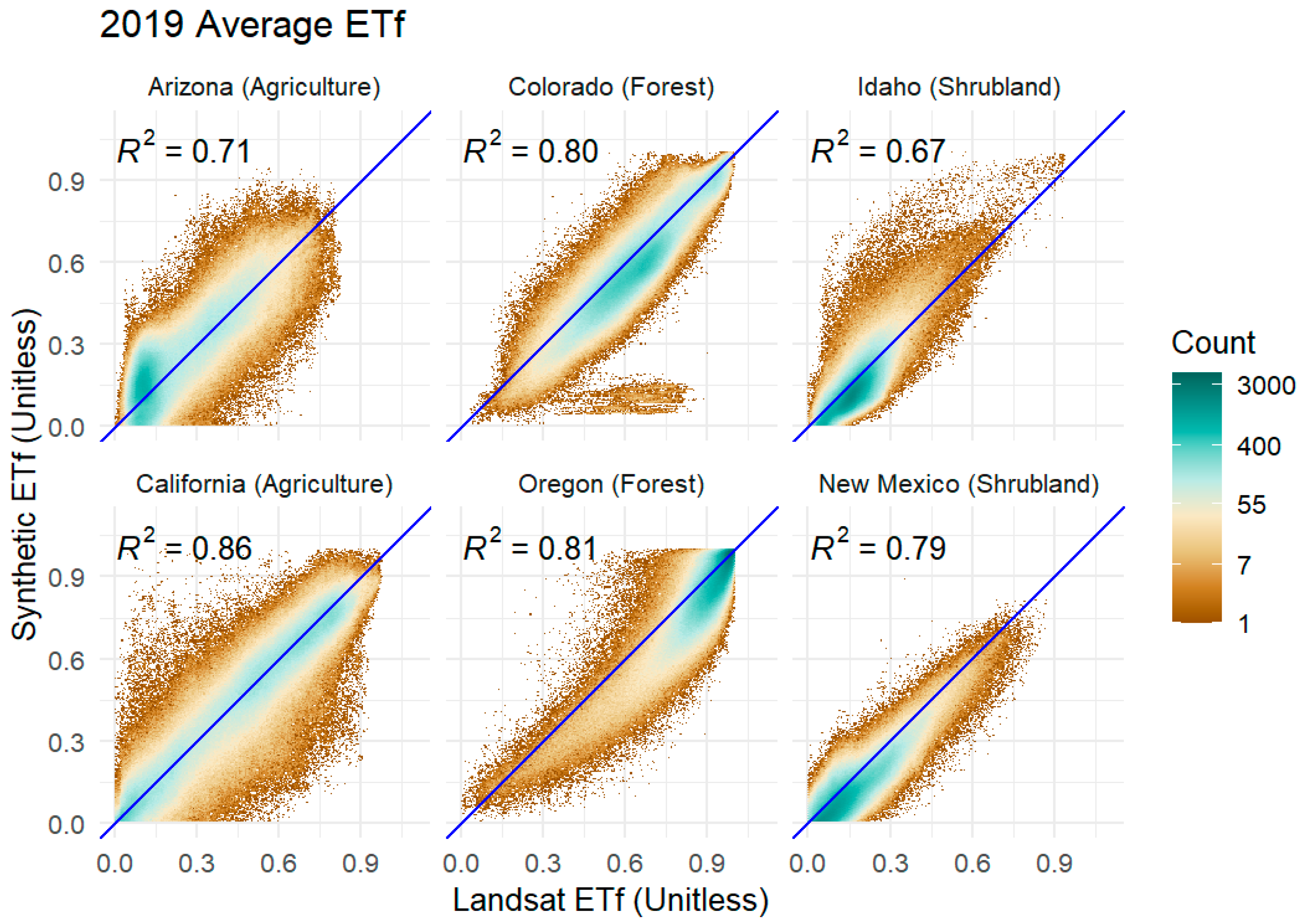
3.2. Evapotranspiration Fraction

The calculation of ETf (Equation (1)) normalizes the LST data into a unitless metric, leading to a much closer match between the synthetic data and those of the observations from Landsat, and minimizes the effects of weather. The synthetic ETf generally matched the annual cycles across 2019 (Figure 5) and only slightly underestimated the ETf from Landsat, particularly for the summer months. Even at the Idaho target area, where the synthetic LST estimates did not closely match the observed LST, the synthetic ETf closely matched the Landsat ETf observations. At the forested target area in Oregon, in addition to underestimating the observed ETf there were also variations in the synthetic ETf that were not apparent in the observed ETf as the result of noise in the synthetic LST data (Figure 3). These underestimates in ETf appeared due to the steeper regression slope in the inverse relationship between the synthetic LST and NDVI data than was apparent in the observations, leading to an underestimation of Tc (Equation (1)) in the synthetic data through the FANO approach [20].
Target-area-wide averages of ETf for 2019 (Figure 6) also showed that synthetic data can produce reasonable ETf estimates and minimize the differences between annual averages of the synthetic data and Landsat observations (Table 2). As shown in Figure 6, the synthetic ETf more closely matched the Landsat observations along the 1:1 line for the New Mexico and California target areas than it did for LST. For the forested Oregon target area, the synthetic ETf underestimated the Landsat observations while closely matching the observed ETf in the Colorado target area. In the Idaho target area, the bulk of the observations followed the 1:1 line; however, there were a considerable number of outliers where the synthetic ETf overestimated the Landsat observations. These outliers appeared to be associated with the steep terrain surrounding the rivers in the Idaho target area. The Arizona target area showed a good fit between the synthetic ETf and Landsat observations for the croplands and an overestimation for the desert regions within the target area. Finally, the magnitude of the RMSE between the synthetic ETf and observed ETf (Table 3) was considerably smaller than that for the LST, indicating that the synthetic ETf estimates were a much better match to the Landsat estimates than LST.

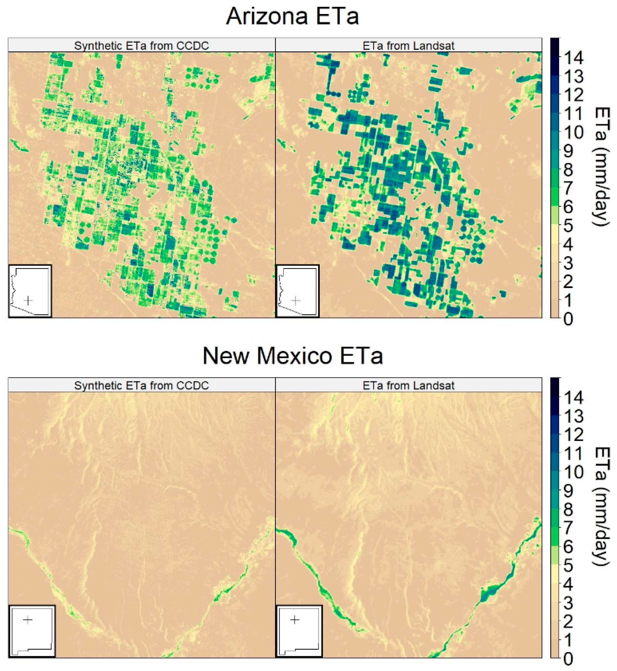
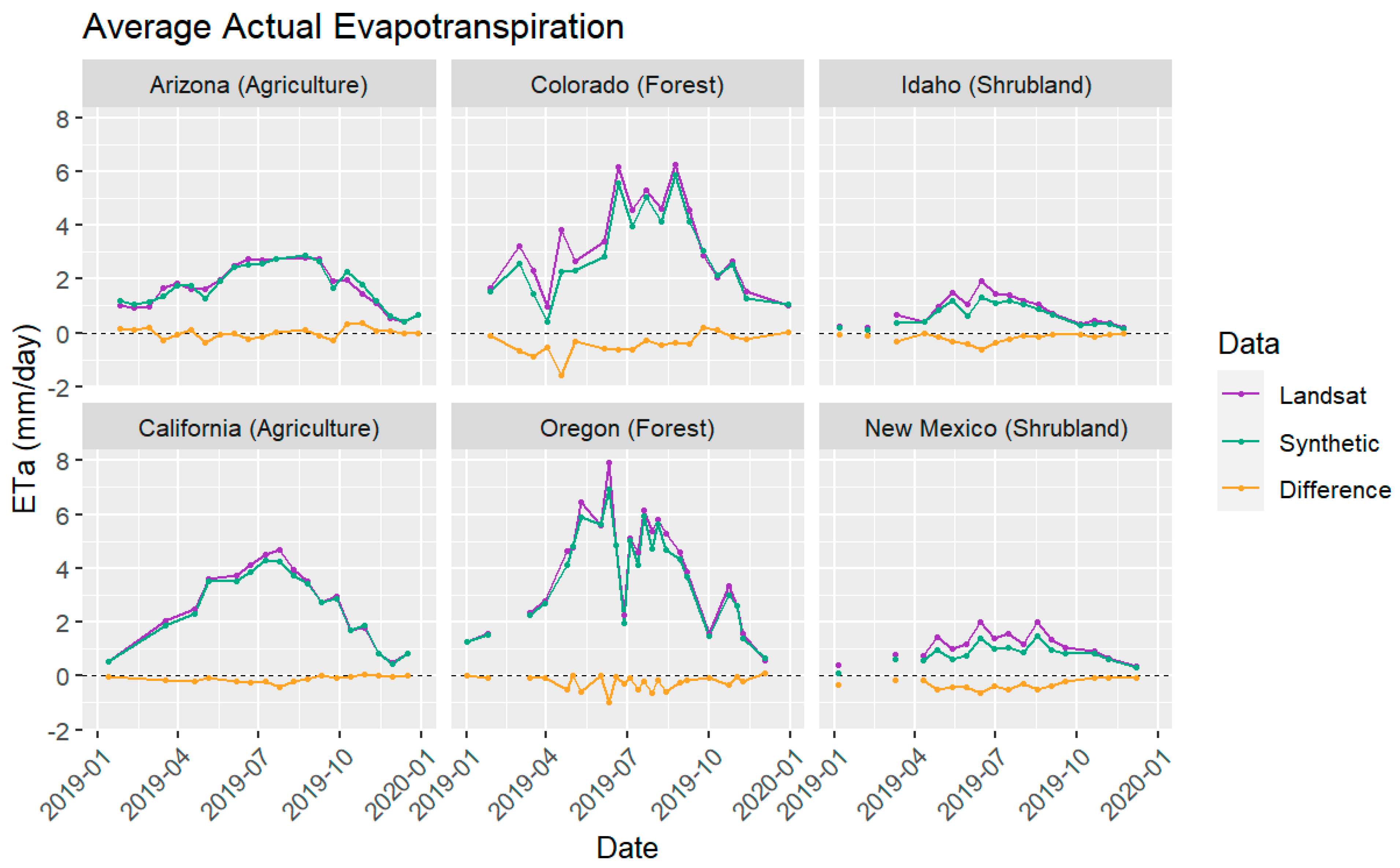
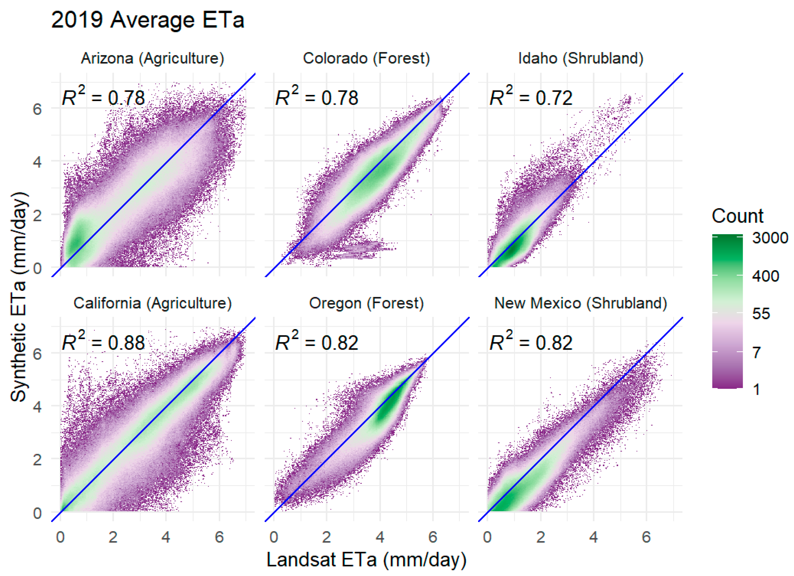
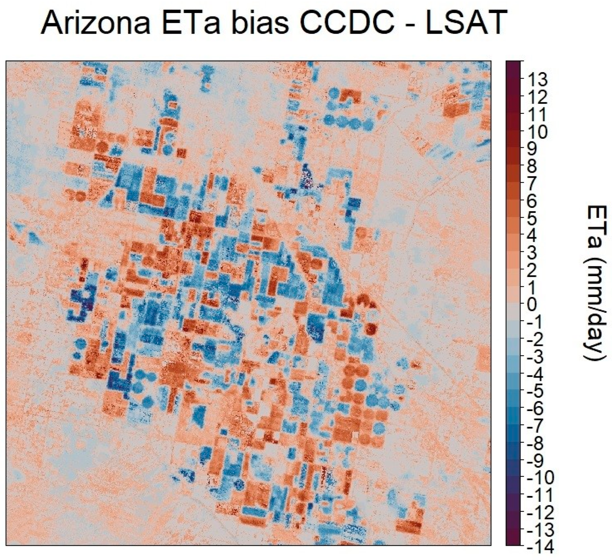
3.3. Actual Evapotranspiration

Side-by-side comparisons of synthetic ETa and observed ETa estimates from Landsat (Figure 7) showed that the synthetically derived data can accurately depict regions of high and low ETa. However, as was the case with LST and ETf, the synthetic ETa typically underestimated the observed ETa. The one exception to this general underestimation by the synthetic ETa data occurred in the desert areas of the Arizona target area, where the synthetic ETa overestimated the observed ETa (Figure 7 and Table 2), while still underestimating ETa in the agricultural areas.
Time series of target area averages (Figure 8) of synthetic and Landsat-derived ETa showed that the synthetic ETa from CCDC accurately depicted seasonal cycles at all six target areas. Additionally, because the ETf was multiplied by gridMet reference evapotranspiration (Equation (2)), the synthetic ETa depicted variations due to weather that were present in the Landsat ETa estimates. However, the synthetic ETa generally underestimated the observed ETa during June, July, and August, with the greatest differences in the Idaho and New Mexico target areas. The forested Colorado target area showed an underestimation by the synthetic ETa in the winter months at the start of 2019, likely the result of winter snow cover. The cropland target areas of California and Arizona showed the closest matches between the synthetic ETa and Landsat observations. The synthetic ETa for the forested Oregon target area closely matched the Landsat-derived ETa, unlike the evaporative fraction, due to the ETr values from gridMet.
At the annual timescale, the 2019 averages of synthetic ETa generally matched those of the observed ETa (Figure 9); however, there was a slight underestimate by the synthetic ETa (Table 2). The synthetic ETa data performed best for the agricultural regions in the California and Arizona target areas. The synthetic ETa slightly underestimated the observed ETa for the shrubland target areas of Idaho and New Mexico. The underestimation of synthetic ETa was most apparent in the forested target area in Colorado and shrubland target area in New Mexico (Table 2). Finally, the overestimation by the synthetic ETa in the Arizona desert region can be seen in the lower left of the Arizona panel in Figure 9, based on the data averaged across all of 2019.

4. Discussion

Synthetic LST and NDVI values from CCDC led to reasonable synthetic ETa estimates at all six target areas for the non-cloud-contaminated pixels. Although CCDC can produce synthetic land cover data for cloud-contaminated pixels, the derived LST and ETa estimates were unreliable. Clouds decreased both LST and ETa by blocking incoming solar radiation and reducing net radiation. The CCDC algorithm does not account for the influence of clouds on net radiation. Thus, we elected to mask out the cloud-contaminated pixels in the synthetic datasets, as indicated by the data gaps in Figure 3, Figure 5 and Figure 8, to focus on the reliable cloud-free data.
These synthetic ETa estimates were more accurate than their corresponding synthetic LST estimates because SSEBop depends on the magnitude of the difference between the hot and cold pixels in each target area to calculate the ETf (Equation (1)) and not the absolute LST values. Additionally, Equation (1) normalized the synthetic LST data and Landsat LST data into the ETf, which ranges from 0 to 1, and further minimized the differences between the synthetic and Landsat data, as indicated by the decrease in RMSE between LST and ETf (Table 3). The accurate synthetic ETf data then led to accurate synthetic ETa estimates when multiplied by the reference evapotranspiration from gridMet (Equation (2)).
At sufficiently large temporal and spatial scales, differences between the average synthetic ETa and average Landsat ETa estimates were less than 1 mm/day. Although accurate at large spatial and temporal scales, these synthetic ETa estimates should not be used for daily weather forecasting or at small spatial scales for individual agricultural fields. The harmonic regression used by CCDC does not capture the variations in ETa that result from irrigation (Figure 10). At both the California and Arizona cropland target areas, irrigation of individual fields shortly before the Landsat flyover resulted in lower LST values, which led to an increase in ETa that was not depicted in the synthetic LST or ETa data. Similarly, fields that were not recently irrigated exhibited higher LSTs and lower ETa values than those predicted by the synthetic datasets from CCDC. However, these spatial variations from irrigation can be averaged across the entire 900 km2 target area (Figure 8) to produce phenologically accurate ETa estimates across the entire year (Figure 9). Additionally, annual averages of the synthetic ETa data produced spatially consistent ETa estimates (Figure 7). The spatial anomalies between the synthetic ETa estimates and observed ETa were less apparent in the shrubland and forest land cover types than in the croplands, as no irrigation occurred in shrubland and forest land. Additionally, the accuracy of the synthetic ETa data had a seasonal component. Across all six target areas, the synthetic ETa values most closely matched the Landsat ETa estimates during the spring and fall, while peak ETa was underestimated during the summer months.
Future work could focus on improving the harmonic CCDC model used for producing synthetic LST and NDVI data to better match summertime Landsat observations before eventually testing its ability to make sub-seasonal ETa forecasts. More accurate synthetic LST and NDVI data may result in a regression line that more closely resembles that in the observed data and allow for more accurate synthetic ETf estimates through FANO [20], ultimately leading to more accurate synthetic ETa data. To improve the accuracy of the synthetic summer and winter time LST and NDVI values, the synthetic harmonic regression could be rerun with an improved fitting algorithm that better captures the seasonal peaks and troughs in the Landsat data. Another modeling approach that could be applied to improve the synthetic ETa data is to begin with the minimum and maximum values as fixed parameters, and then estimate the sub-annual changes as damped oscillations between these extrema [44]. Rerunning the harmonic regression on a shorter timeframe, as opposed to the LCMAP study period, may improve its ability to capture peak summertime values and thus eliminate the underestimation of summer ETa. Another approach that could improve CCDC’s ability to generate accurate synthetic data for SSEBop would be to run the harmonic regression on Landsat-derived LST data [45] to generate synthetic LST, as opposed to using the synthetic surface brightness temperatures to generate the synthetic LST values required for SSEBop.
It is important to note that this research has identified several potential problems that may arise when transitioning to an operations setting, in which a continuous stream of ETa estimates is provided to end users. One large issue is related to systematic bias in Ts, Tc, ETf, and/or ETa. In addition to potential improvements in the CCDC algorithm, as discussed above, future research could also explore more detailed, long-period (1980s to present) ETa estimates for a few key sites. A deeper historical record could enable more detailed evaluation of the causes of biases. The other main issue that has been raised in this paper is the potential for very large ETa errors when there is a mis-match between the irrigation status of farmland. To potentially address this issue, future research could explore the possibility of dynamically updating the CCDC data to more closely represent current conditions.
The work presented here illustrates the ability of synthetic land cover data from CCDC to generate accurate ETa estimates, paving the way for new approaches to generate near-term ETa forecasts. Once the fitting algorithm has been improved, the harmonic regression model can be used to generate synthetic land surface data to produce SSEBop-derived ETa estimates between Landsat overpasses and validated against flux tower observations. An immediate application of the improved synthetic ETa estimates would be to combine them with real data to investigate irrigation practices in arid regions, because subtracting the real data from the synthetic data clearly highlights irrigation patterns (Figure 10). Then, to make sub-seasonal ETa predictions, the harmonic regression model could be combined with meteorological imputes from the Parameter-elevation Regressions on Independent Slopes Model (PRISM) [46] and extended six weeks into the future with a machine learning approach. Combining the improved harmonic regression model for detecting land change along with PRISM data through a machine learning approach may lead to high-quality land cover predictions that could ultimately result in quality ETa forecasts when coupled with SSEBop.

5. Conclusions

In conclusion, this study used CCDC data to generate synthetic Landsat data that were then used to initialize SSEBop. The CCDC-derived synthetic ETa estimates were validated against Landsat estimates at six target areas in the western United States, representing forests, croplands, and shrubland land cover types. Synthetic ETf estimates provided much closer matches to the Landsat data than those observed in LST because the ETf estimations depend on the relative distributions in LST rather than the absolute magnitude in LST, which substantially enhances performance. The synthetic ETa accurately depicted regions of high and low evapotranspiration and seasonal variations in ETa. However, the synthetic ETa typically underestimated peak summer ETa, while providing a much closer match to the Landsat ETa estimates in fall and spring. Additionally, the synthetic ETa does not reflect ETa variations due to changing irrigation practices from irrigation in agricultural areas. Future work could focus improving the harmonic fitting algorithm to better capture summertime ETa values and combine CCDC with meteorological data through machine learning to provide enhanced projections of ETa. Using CCDC to generate ETa forecasts may allow for enhanced drought prediction, allowing stakeholders and decision-makers to make more informed water management decisions in the increasingly water-stressed western United States.

Author Contributions

Conceptualization, M.P.H., H.J.T. and C.F.; methodology, M.P.H., H.J.T., C.F. and G.B.S.; software, M.P.H., K.C.F. and M.O.F.; validation, M.P.H., H.J.T., C.F. and G.B.S.; formal analysis, M.P.H.; investigation, M.P.H.; writing—original draft preparation, M.P.H.; writing—review and editing, M.P.H., H.J.T., C.F., G.B.S. and M.O.F.; visualization, M.P.H. All authors have read and agreed to the published version of the manuscript.

Funding

Funding was provided through the Mendenhall Postdoctoral Fellowship program of the U.S. Geological Survey. The authors declare that no additional funds, grants, or other support were received during the preparation of this manuscript.

Data Availability Statement

The Landsat images used in the study are freely available online through Earth Explorer at https://earthexplorer.usgs.gov/ (accessed on 4 April, 2023). The SSEBop code is available on GitHub at: https://github.com/Open-ET/openet-ssebop (accessed on 14 April 2023). LCMAP data are available online through Earth Explorer at: https://earthexplorer.usgs.gov/ (accessed on 12 April 2023), and Crop Scape data are available online through the USDA at: https://nassgeodata.gmu.edu/CropScape/ (accessed on 12 April 2023) [42]. The synthetic CCDC data generated during this study and CCDC code are available upon request.

Acknowledgments

Thanks to Shraddhanand Shukla for the insights on gridMet and reference evapotranspiration and Seamus O’Neil for the line editing. Any use of trade, firm, or product names is for descriptive purposes only and does not imply endorsement by the U.S. Government.

Conflicts of Interest

The authors declare no conflicts of interest.

References

  1. Anderson, M.C.; Hain, C.; Wardlow, B.; Pimstein, A.; Mecikalski, J.R.; Kustas, W.P. Evaluation of Drought Indices Based on Thermal Remote Sensing of Evapotranspiration over the Continental United States. J. Clim. 2011, 24, 2025–2044. [Google Scholar] [CrossRef]
  2. Aghakouchak, A.; Farahmand, A.; Melton, F.S.; Teixeira, J.; Anderson, M.C.; Wardlow, B.D.; Hain, C.R. Reviews of Geophysics Remote Sensing of Drought: Progress, Challenges. Rev. Geophys. 2015, 53, 452–480. [Google Scholar] [CrossRef]
  3. Gavahi, K.; Abbaszadeh, P.; Moradkhani, H.; Zhan, X.; Hain, C. Multivariate Assimilation of Remotely Sensed Soil Moisture and Evapotranspiration for Drought Monitoring. J. Hydrometeorol. 2020, 21, 2293–2308. [Google Scholar] [CrossRef]
  4. Knipper, K.R.; Kustas, W.P.; Anderson, M.C.; Alfieri, J.G.; Prueger, J.H.; Hain, C.R.; Gao, F.; Yang, Y.; McKee, L.G.; Nieto, H.; et al. Evapotranspiration Estimates Derived Using Thermal-Based Satellite Remote Sensing and Data Fusion for Irrigation Management in California Vineyards. Irrig. Sci. 2019, 37, 431–449. [Google Scholar] [CrossRef]
  5. Roche, J.W.; Ma, Q.; Rungee, J.; Bales, R.C. Evapotranspiration Mapping for Forest Management in California’s Sierra Nevada. Front. For. Glob. Chang. 2020, 3, 69. [Google Scholar] [CrossRef]
  6. Niyogi, D.; Jamshidi, S.; Smith, D.; Kellner, O. Evapotranspiration Climatology of Indiana Using In Situ and Remotely Sensed Products. J. Appl. Meteorol. Climatol. 2020, 50, 2093–2111. [Google Scholar] [CrossRef]
  7. Anderson, M.C.; Norman, J.M.; Mecikalski, J.R.; Otkin, J.A.; Kustas, W.P. A Climatological Study of Evapotranspiration and Moisture Stress across the Continental United States Based on Thermal Remote Sensing: 1. Model Formulation. J. Geophys. Res. Atmos. 2007, 112. [Google Scholar] [CrossRef]
  8. Senay, G.B.; Bohms, S.; Singh, R.K.; Gowda, P.H.; Velpuri, N.M.; Alemu, H.; Verdin, J.P. Operational Evapotranspiration Mapping Using Remote Sensing and Weather Datasets: A New Parameterization for the SSEB Approach. J. Am. Water Resour. Assoc. 2013, 49, 577–591. [Google Scholar] [CrossRef]
  9. Melton, F.S.; Huntington, J.; Grimm, R.; Herring, J.; Hall, M.; Rollison, D.; Erickson, T.; Allen, R.; Anderson, M.; Fisher, J.B.; et al. OpenET: Filling a Critical Data Gap in Water Management for the Western United States. J. Am. Water Resour. Assoc. 2022, 58, 971–994. [Google Scholar] [CrossRef]
  10. Fisher, J.B.; Lee, B.; Purdy, A.J.; Halverson, G.H.; Dohlen, M.B.; Cawse-Nicholson, K.; Wang, A.; Anderson, R.G.; Aragon, B.; Arain, M.A.; et al. ECOSTRESS: NASA’s Next Generation Mission to Measure Evapotranspiration From the International Space Station. Water Resour. Res. 2020, 56, e2019WR026058. [Google Scholar] [CrossRef]
  11. Pelosi, A.; Medina, H.; Villani, P.; D’Urso, G.; Chirico, G.B. Probabilistic Forecasting of Reference Evapotranspiration with a Limited Area Ensemble Prediction System. Agric. Water Manag. 2016, 178, 106–118. [Google Scholar] [CrossRef]
  12. Perera, K.C.; Western, A.W.; Nawarathna, B.; George, B. Forecasting Daily Reference Evapotranspiration for Australia Using Numerical Weather Prediction Outputs. Agric. For. Meteorol. 2014, 194, 50–63. [Google Scholar] [CrossRef]
  13. Medina, H.; Tian, D.; Srivastava, P.; Pelosi, A.; Chirico, G.B. Medium-Range Reference Evapotranspiration Forecasts for the Contiguous United States Based on Multi-Model Numerical Weather Predictions. J. Hydrol. 2018, 562, 502–517. [Google Scholar] [CrossRef]
  14. Karbasi, M. Forecasting of Multi-Step Ahead Reference Evapotranspiration Using Wavelet- Gaussian Process Regression Model. Water Resour. Manag. 2018, 32, 1035–1052. [Google Scholar] [CrossRef]
  15. de Oliveira e Lucas, P.; Alves, M.A.; de Lima e Silva, P.C.; Guimarães, F.G. Reference Evapotranspiration Time Series Forecasting with Ensemble of Convolutional Neural Networks. Comput. Electron. Agric. 2020, 177, 105700. [Google Scholar] [CrossRef]
  16. Ferreira, L.B.; da Cunha, F.F. Multi-Step Ahead Forecasting of Daily Reference Evapotranspiration Using Deep Learning. Comput. Electron. Agric. 2020, 178, 105728. [Google Scholar] [CrossRef]
  17. McEvoy, D.J.; Huntington, J.L.; Mejia, J.F.; Hobbins, M.T. Improved Seasonal Drought Forecasts Using Reference Evapotranspiration Anomalies. Geophys. Res. Lett. 2016, 43, 377–385. [Google Scholar] [CrossRef]
  18. Blankenau, P.A.; Kilic, A.; Allen, R. An Evaluation of Gridded Weather Data Sets for the Purpose of Estimating Reference Evapotranspiration in the United States. Agric. Water Manag. 2020, 242, 106376. [Google Scholar] [CrossRef]
  19. Zhu, Z.; Woodcock, C.E. Continuous Change Detection and Classification of Land Cover Using All Available Landsat Data. Remote Sens. Environ. 2014, 144, 152–171. [Google Scholar] [CrossRef]
  20. Senay, G.B.; Parrish, G.E.L.; Schauer, M.; Friedrichs, M.; Khand, K.; Boiko, O.; Kagone, S.; Dittmeier, R.; Arab, S.; Ji, L. Improving the Operational Simplified Surface Energy Balance Evapotranspiration Model Using the Forcing and Normalizing Operation. Remote Sens. 2023, 15, 260. [Google Scholar] [CrossRef]
  21. Bastiaanssen, W.G.M.; Pelgrum, H.; Wang, J.; Ma, Y.; Moreno, J.F.; Roerink, G.J.; Van Der Wal, T. A Remote Sensing Surface Energy Balance Algorithm for Land (SEBAL): 2. Validation. J. Hydrol. 1998, 212–213, 213–229. [Google Scholar] [CrossRef]
  22. Allen, R.G.; Tasumi, M.; Morse, A.; Trezza, R.; Wright, J.L.; Bastiaanssen, W.; Kramber, W.; Lorite, I.; Robison, C.W. Satellite-Based Energy Balance for Mapping Evapotranspiration with Internalized Calibration (METRIC)—Applications. J. Irrig. Drain. Eng. 2007, 133, 395–406. [Google Scholar] [CrossRef]
  23. Hersbach, H.; Bell, B.; Berrisford, P.; Hirahara, S.; Horányi, A.; Muñoz-Sabater, J.; Nicolas, J.; Peubey, C.; Radu, R.; Schepers, D.; et al. The ERA5 Global Reanalysis. Q. J. R. Meteorol. Soc. 2020, 146, 1999–2049. [Google Scholar] [CrossRef]
  24. Abatzoglou, J.T. Development of Gridded Surface Meteorological Data for Ecological Applications and Modelling. Int. J. Climatol. 2013, 33, 121–131. [Google Scholar] [CrossRef]
  25. Anderson, M.C.; Yang, Y.; Xue, J.; Knipper, K.R.; Yang, Y.; Gao, F.; Hain, C.R.; Kustas, W.P.; Cawse-Nicholson, K.; Hulley, G.; et al. Interoperability of ECOSTRESS and Landsat for Mapping Evapotranspiration Time Series at Sub-Field Scales. Remote Sens. Environ. 2021, 252, 112189. [Google Scholar] [CrossRef]
  26. de Paula, A.C.P.; da Silva, C.L.; Rodrigues, L.N.; Scherer-Warren, M. Performance of the SSEBop Model in the Estimation of the Actual Evapotranspiration of Soybean and Bean Crops. Pesqui. Agropecu. Bras. 2019, 54, e00739. [Google Scholar] [CrossRef]
  27. Dias Lopes, J.; Neiva Rodrigues, L.; Acioli Imbuzeiro, H.M.; Falco Pruski, F. Performance of SSEBop Model for Estimating Wheat Actual Evapotranspiration in the Brazilian Savannah Region. Int. J. Remote Sens. 2019, 40, 6930–6947. [Google Scholar] [CrossRef]
  28. Ayyad, S.; Al Zayed, I.S.; Ha, V.T.T.; Ribbe, L. The Performance of Satellite-Based Actual Evapotranspiration Products and the Assessment of Irrigation Efficiency in Egypt. Water 2019, 11, 1913. [Google Scholar] [CrossRef]
  29. Senay, G.B.; Schauer, M.; Friedrichs, M.; Velpuri, N.M.; Singh, R.K. Satellite-Based Water Use Dynamics Using Historical Landsat Data (1984–2014) in the Southwestern United States. Remote Sens. Environ. 2017, 202, 98–112. [Google Scholar] [CrossRef]
  30. Senay, G.B.; Friedrichs, M.; Morton, C.; Parrish, G.E.L.; Schauer, M.; Khand, K.; Kagone, S.; Boiko, O.; Huntington, J. Mapping Actual Evapotranspiration Using Landsat for the Conterminous United States: Google Earth Engine Implementation and Assessment of the SSEBop Model. Remote Sens. Environ. 2022, 275, 113011. [Google Scholar] [CrossRef]
  31. Crawford, C.J.; Roy, D.P.; Arab, S.; Barnes, C.; Vermote, E.; Hulley, G.; Gerace, A.; Choate, M.; Engebretson, C.; Micijevic, E.; et al. The 50-Year Landsat Collection 2 Archive. Sci. Remote Sens. 2023, 8, 100103. [Google Scholar] [CrossRef]
  32. Roy, D.P.; Wulder, M.A.; Loveland, T.R.; Woodcock, C.E.; Allen, R.G.; Anderson, M.C.; Helder, D.; Irons, J.R.; Johnson, D.M.; Kennedy, R.; et al. Landsat-8: Science and Product Vision for Terrestrial Global Change Research. Remote Sens. Environ. 2014, 145, 154–172. [Google Scholar] [CrossRef]
  33. Dwyer, J.L.; Roy, D.P.; Sauer, B.; Jenkerson, C.B.; Zhang, H.K.; Lymburner, L. Analysis Ready Data: Enabling Analysis of the Landsat Archive. Remote Sens. 2018, 10, 1363. [Google Scholar] [CrossRef]
  34. Vermote, E.; Justice, C.; Claverie, M.; Franch, B. Preliminary Analysis of the Performance of the Landsat 8/OLI Land Surface Reflectance Product. Remote Sens. Environ. 2016, 185, 46–56. [Google Scholar] [CrossRef] [PubMed]
  35. Lewis, A.; Lacey, J.; Mecklenburg, S.; Ross, J.; Siqueira, A.; Killough, B.; Szantoi, Z.; Tadono, T.; Rosenqvist, A.; Goryl, P.; et al. CEOS Analysis Ready Data for Land (CARD4L) Overview. In Proceedings of the IGARSS 2018—2018 IEEE International Geoscience and Remote Sensing Symposium, Valencia, Spain, 22–27 July 2018; pp. 7407–7410. [Google Scholar]
  36. Xian, G.Z.; Smith, K.; Wellington, D.; Horton, J.; Zhou, Q.; Li, C.; Auch, R.; Brown, J.F.; Zhu, Z.; Reker, R.R. Implementation of the CCDC Algorithm to Produce the LCMAP Collection 1.0 Annual Land Surface Change Product. Earth Syst. Sci. Data 2022, 14, 143–162. [Google Scholar] [CrossRef]
  37. Zhu, Z.; Wang, S.; Woodcock, C.E. Improvement and Expansion of the Fmask Algorithm: Cloud, Cloud Shadow, and Snow Detection for Landsats 4-7, 8, and Sentinel 2 Images. Remote Sens. Environ. 2015, 159, 269–277. [Google Scholar] [CrossRef]
  38. Zhu, Z.; Woodcock, C.E. Object-Based Cloud and Cloud Shadow Detection in Landsat Imagery. Remote Sens. Environ. 2012, 118, 83–94. [Google Scholar] [CrossRef]
  39. Zhu, Z.; Woodcock, C.E.; Holden, C.; Yang, Z. Generating Synthetic Landsat Images Based on All Available Landsat Data: Predicting Landsat Surface Reflectance at Any given Time. Remote Sens. Environ. 2015, 162, 67–83. [Google Scholar] [CrossRef]
  40. Omernik, J.M.; Griffith, G.E. Ecoregions of the Conterminous United States: Evolution of a Hierarchical Spatial Framework. Environ. Manag. 2014, 54, 1249–1266. [Google Scholar] [CrossRef]
  41. Brown, J.F.; Tollerud, H.J.; Barber, C.P.; Zhou, Q.; Dwyer, J.L.; Vogelmann, J.E.; Loveland, T.R.; Woodcock, C.E.; Stehman, S.V.; Zhu, Z.; et al. Lessons Learned Implementing an Operational Continuous United States National Land Change Monitoring Capability: The Land Change Monitoring, Assessment, and Projection (LCMAP) Approach. Remote Sens. Environ. 2020, 238, 111356. [Google Scholar] [CrossRef]
  42. Han, W.; Yang, Z.; Di, L.; Mueller, R. CropScape: A Web Service Based Application for Exploring and Disseminating US Conterminous Geospatial Cropland Data Products for Decision Support. Comput. Electron. Agric. 2012, 84, 111–123. [Google Scholar] [CrossRef]
  43. Tibshiranit, R. Regression Shrinkage and Selection via the Lasso. J. R. Statist. Soc. B 1996, 58, 267–288. [Google Scholar]
  44. Funk, C.; Budde, M.E. Phenologically-Tuned MODIS NDVI-Based Production Anomaly Estimates for Zimbabwe. Remote Sens. Environ. 2009, 113, 115–125. [Google Scholar] [CrossRef]
  45. Cook, M.; Schott, J.R.; Mandel, J.; Raqueno, N. Development of an Operational Calibration Methodology for the Landsat Thermal Data Archive and Initial Testing of the Atmospheric Compensation Component of a Land Surface Temperature (LST) Product from the Archive. Remote Sens. 2014, 6, 11244–11266. [Google Scholar] [CrossRef]
  46. Daly, C.; Gibson, W.P.; Taylor, G.H.; Johnson, G.L.; Pasteris, P. A Knowledge-Based Approach to the Statistical Mapping of Climate. Clim. Res. 2002, 22, 99–113. [Google Scholar] [CrossRef]
Figure 1. The locations of the six target areas (white dots) in the western United States and their associated ecoregions. The Level I ecoregion data are available at ecologicalregions.info/htm/na_eco.htm (accessed on 23 February 2024).
Remotesensing 16 01297 g001
Figure 2. Red, green, and blue composite Landsat images of the six target areas. The Arizona target area (a) consists of irrigated croplands and desert. The California target area (b) consist mostly of irrigated almond plantations. Both the Colorado (c) and Oregon (d) target areas are largely forested. Then, both the Idaho (e) and New Mexico (f) target areas are shrubland.
Remotesensing 16 01297 g002
Figure 3. Target-area-wide averages of the Landsat (purple) and synthetic (cyan) land surface temperature (LST) estimates for 2019. The yellow difference line represents the Landsat data minus the synthetic data at each timestep. Note that the gaps in both the Landsat and synthetic data were the result of applying the same Landsat cloud mask to both datasets.
Remotesensing 16 01297 g003
Figure 4. Heat plots of synthetic land surface temperature (LST), derived from Continuous Change Detection and Classification (CCDC) and Landsat LST estimations for 2019, showing a per-pixel comparison for each target area. The blue 1:1 line represents the hypothetical perfect fit between observed LST and synthetic LST. Note the logarithmic scale, with purple indicating high pixel counts and orange indicating low pixel counts. Linear regression results are indicated by the R2 values and are significant at p < 0.001.
Remotesensing 16 01297 g004
Figure 5. Target-area-wide averages of the Landsat (purple) and synthetic (cyan) evaporative fraction (ETf) estimates for 2019. The yellow difference line represents the Landsat data minus the synthetic data at each timestep. Note that the gaps in both the Landsat and synthetic data were the result of applying the same Landsat cloud mask to both datasets.
Remotesensing 16 01297 g005
Figure 6. Heat plots of synthetic evaporative fraction (ETf), derived from Continuous Change Detection and Classification (CCDC) and Landsat ETf estimations for 2019, showing a per-pixel comparison for each target area. The blue 1:1 line represents the hypothetical perfect fit between observed ETf and synthetic ETf. Note the logarithmic scale, with green indicating high pixel counts and brown indicating low pixel counts. Linear regression results are indicated by the R2 values and are significant at p < 0.001.
Remotesensing 16 01297 g006
Figure 7. Side-by-side comparisons of the synthetic actual evapotranspiration (ETa) data (left) derived from the Continuous Change Detection and Classification (CCDC) and the observed ETa from Landsat (right). The Arizona (top) data correspond to a Landsat overpass on 5 July 2019, and New Mexico (bottom) data are from an overpass on 30 June 2019. The location of each target area is indicated by the plus sign in the bottom left corner.
Remotesensing 16 01297 g007
Figure 8. Target-area-wide averages of the Landsat (purple) and synthetic (cyan) actual evapotranspiration (ETa) estimates for 2019. The yellow difference line represents the Landsat data minus the synthetic data at each timestep. Note that the gaps in both the Landsat and synthetic data were the result of applying the same Landsat cloud mask to both datasets.
Remotesensing 16 01297 g008
Figure 9. Heat plots of synthetic actual evapotranspiration (ETa), derived from Continuous Change Detection and Classification (CCDC), and Landsat ETa estimations for 2019, showing a per-pixel comparison for each target area. The blue 1:1 line represents the hypothetical perfect fit between observed ETa and synthetic ETa. Note the logarithmic scale, with green indicating high pixel counts and purple indicating low pixel counts. Linear regression results are indicated by the R2 values and are significant at p < 0.001.
Remotesensing 16 01297 g009
Figure 10. Actual evapotranspiration (ETa) bias map showing the synthetic ETa estimates minus the Landsat ETa estimates for 21 July 2019, showing the large amount of spatial variation due to irrigation. The synthetic data underestimated ETa for fields that had recently been irrigated, and high ETa in the Landsat data (blue) and overestimated ETa (red) in agricultural fields that had not been irrigated recently.
Remotesensing 16 01297 g010
Table 1. The county-wide mean temperatures for 2019, along with the mean annual temperature for the 1901–2000 period and the 2019 total precipitation for the six target areas. The 1901–2000 mean precipitation is the average of the yearly total precipitation amounts for 1901–2000. Climate data were courtesy of NOAA National Centers for Environmental information, Climate at a Glance: County Rankings, from: https://www.ncei.noaa.gov/access/monitoring/climate-at-a-glance/county/rankings (accessed on 6 March 2024).
Target AreaCounty2019 Mean Temp1901–2000 Mean Temp2019 Total Precip1901–2000 Mean Precip
ArizonaPinal County20.5 °C19.8 °C 391.16 mm 318.01 mm
CaliforniaKern County16.5 °C15.8 °C 338.33 mm 229.87 mm
ColoradoDolores County6.1 °C5.4 °C 618.49 mm 593.09 mm
OregonLinn County9.4 °C9.2 °C 1420.11 mm 1763.78 mm
IdahoOwyhee County8.3 °C8.2 °C 367.03 mm 319.02 mm
New MexicoSandoval County10.1 °C9.6 °C 303.53 mm 340.11 mm
Table 2. The differences between the 2019 target-area-wide averages in the synthetic Continuous Change Detection and Classification (CCDC) data and the Landsat observations for the land surface temperature (LST), evaporative fraction (ETf), and actual evapotranspiration (ETa) at each target area.
2019 Target Area Wide Average Differences
Study AreaLST (°C)ETfETa (mm/day)
Arizona−1.100.000.01
California−1.61−0.02−0.13
Colorado0.11−0.05−0.30
Oregon−2.70−0.05−0.25
Idaho9.87−0.03−0.18
New Mexico−2.16−0.04−0.32
Table 3. Root mean squared error (RMSE) between the synthetic Continuous Change Detection and Classification (CCDC) data and Landsat observations for the 2019 averages of land surface temperature (LST), evaporative fraction (ETf), and actual evapotranspiration (ETa).
RMSE Error for the 2019 Averages
Study AreaLST (°C)ETfETa mm/day
Arizona3.180.090.68
California2.320.100.60
Colorado1.950.090.53
Oregon3.070.080.39
Idaho9.980.070.33
New Mexico2.570.070.48
Disclaimer/Publisher’s Note: The statements, opinions and data contained in all publications are solely those of the individual author(s) and contributor(s) and not of MDPI and/or the editor(s). MDPI and/or the editor(s) disclaim responsibility for any injury to people or property resulting from any ideas, methods, instructions or products referred to in the content.

