
Spatiotemporal Patterns of Air Pollutants over the Epidemic Course: A National Study in China

 ,
, 
 , ,
, , 
Abstract

1. Introduction
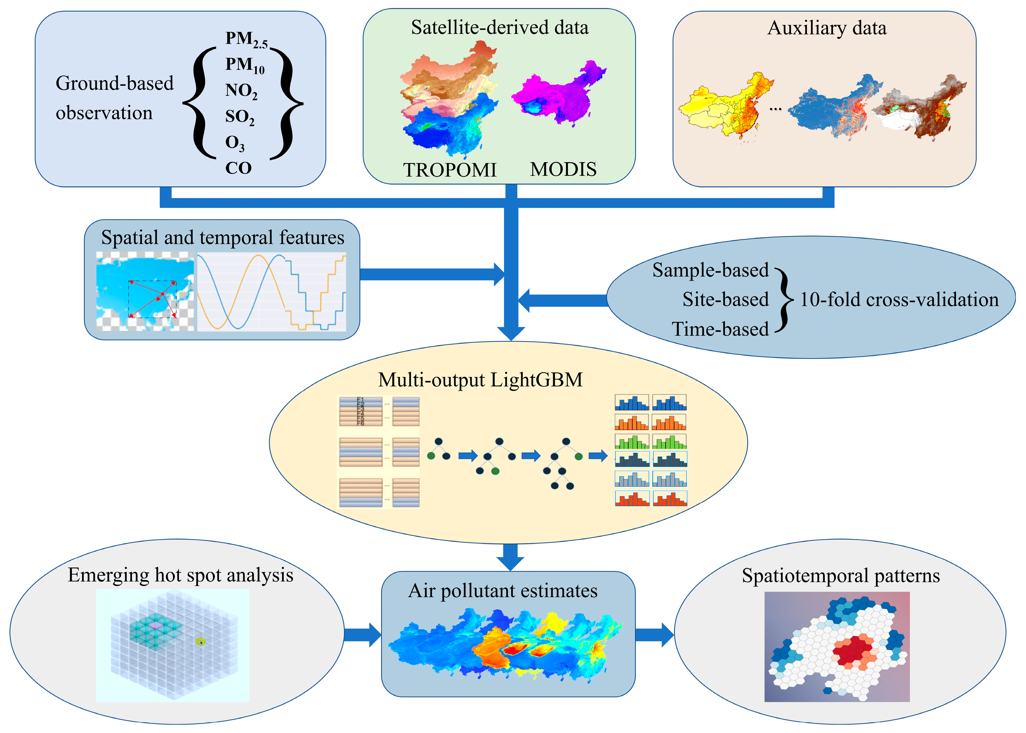
2. Methods
2.1. Datasets
2.1.1. Ground-Based Measurements
2.1.2. Satellite-Derived Data
2.1.3. Auxiliary Data
2.2. Extraction of Spatial and Temporal Features
2.3. Algorithm Description
2.4. Model Evaluation
2.5. Trend Analysis
3. Results
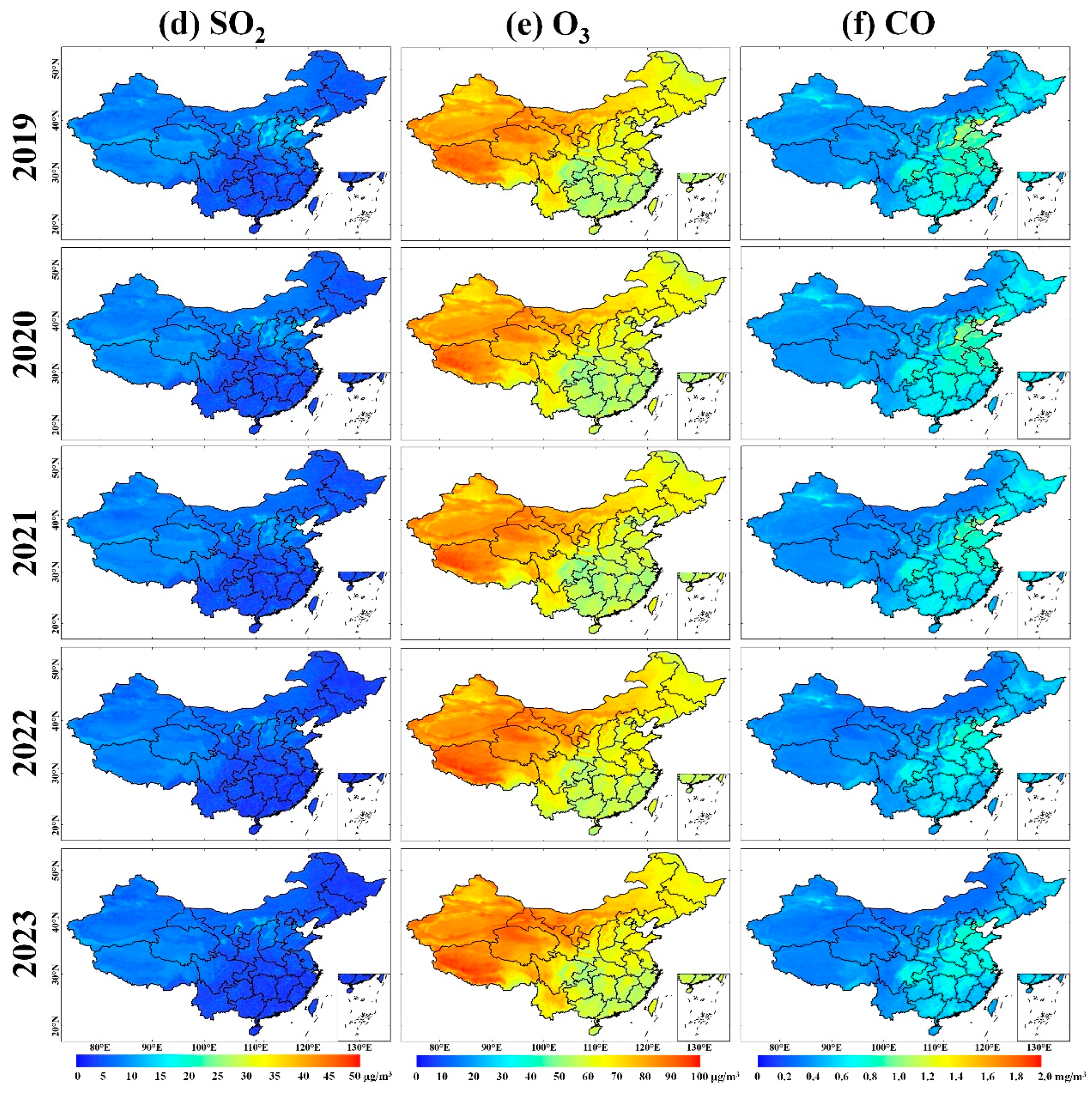
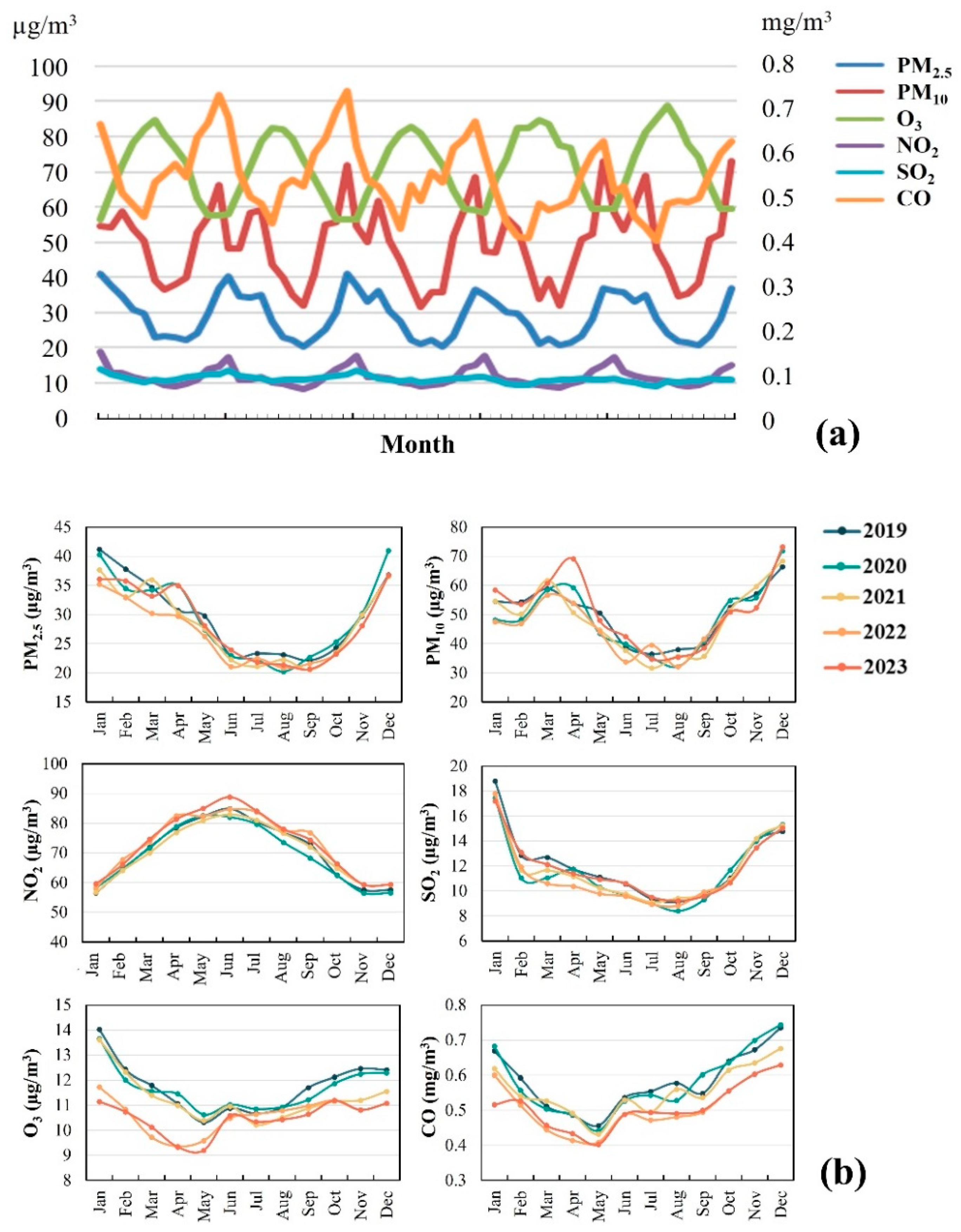
3.1. Spatial and Temporal Distribution of Air Pollutants
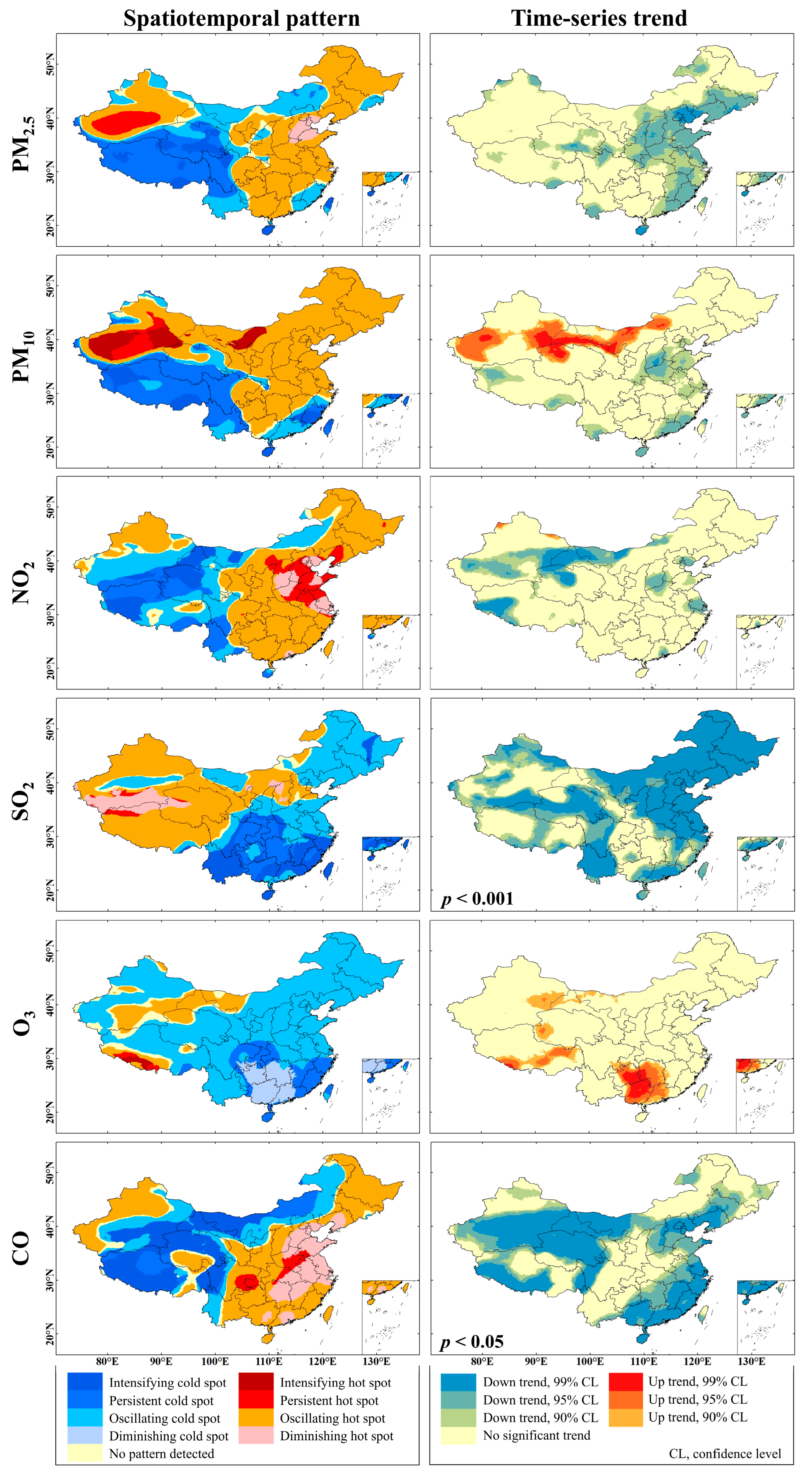
3.2. Spatiotemporal Patterns of Air Pollutants
3.3. Model Performance
3.3.1. Feature Importance of Predictor Variables
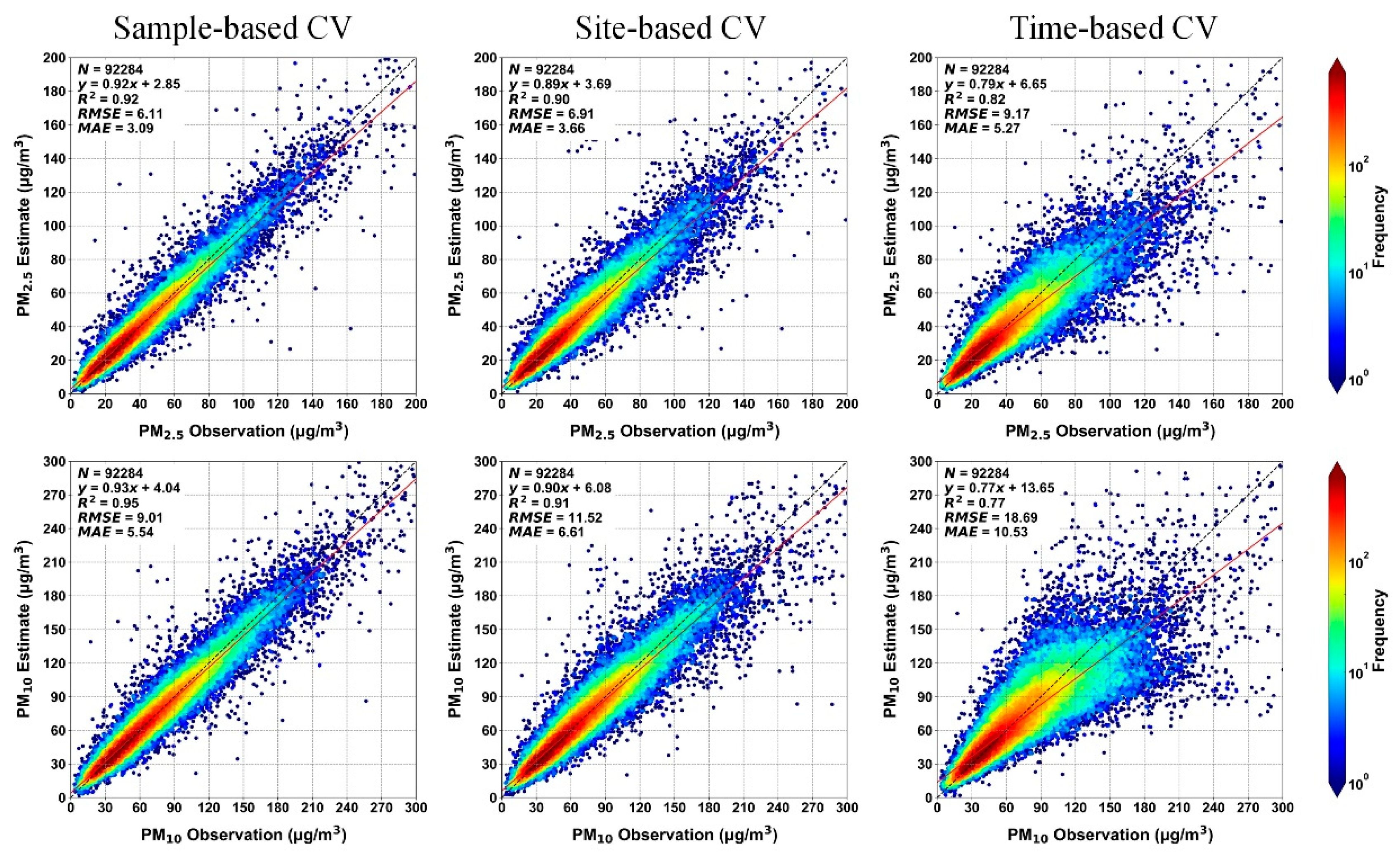
3.3.2. Predictive Accuracy of CV Results
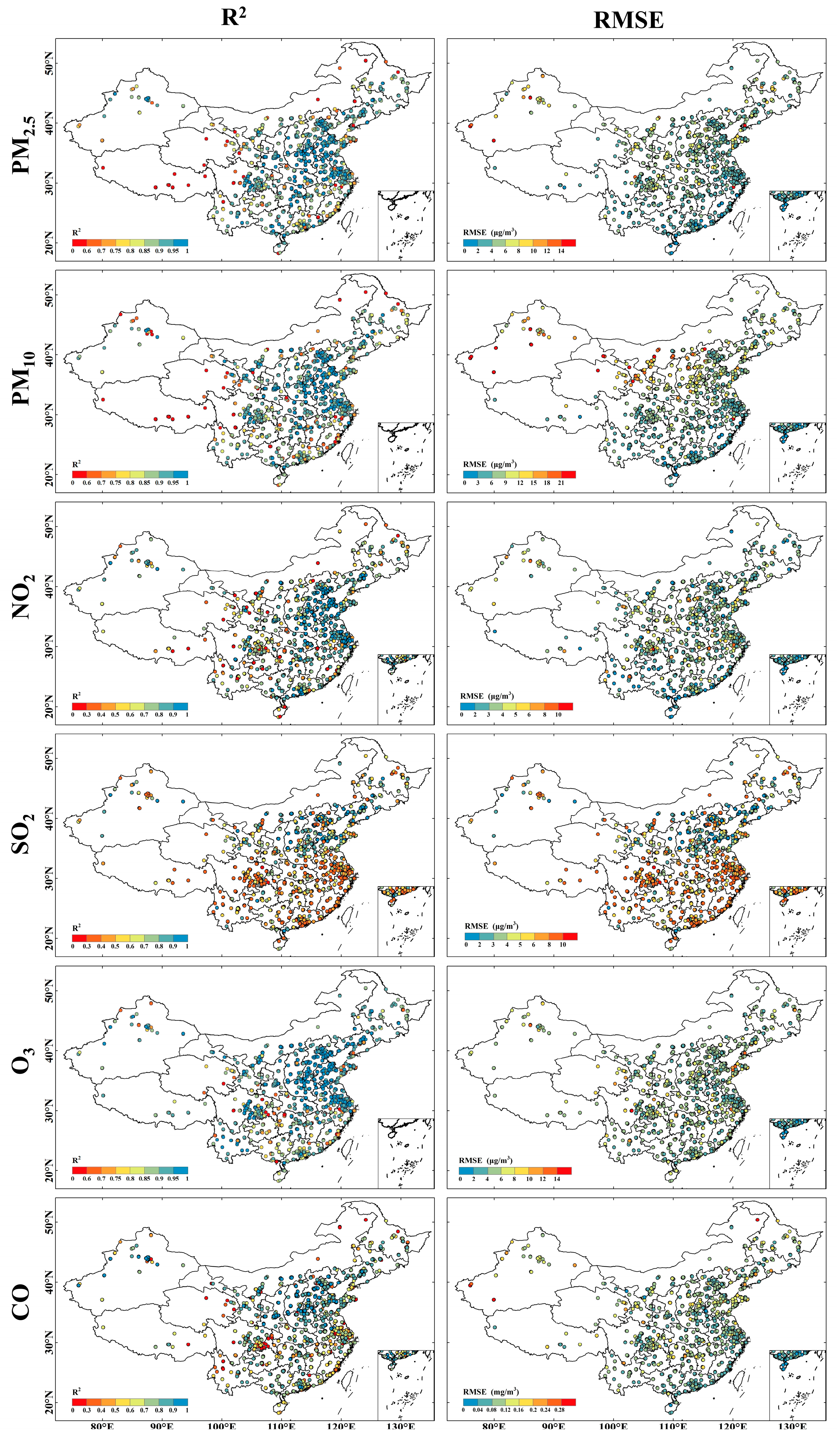
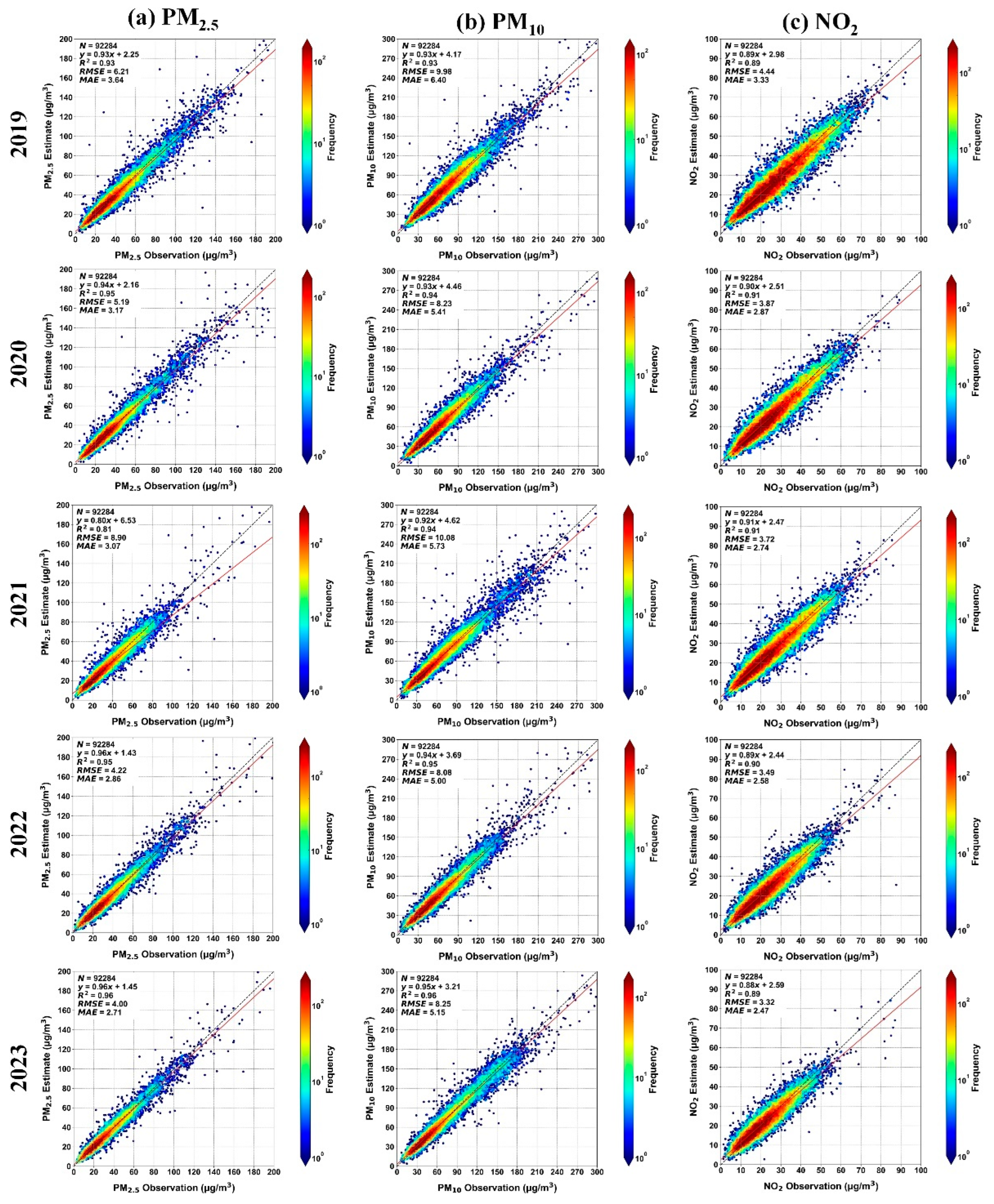
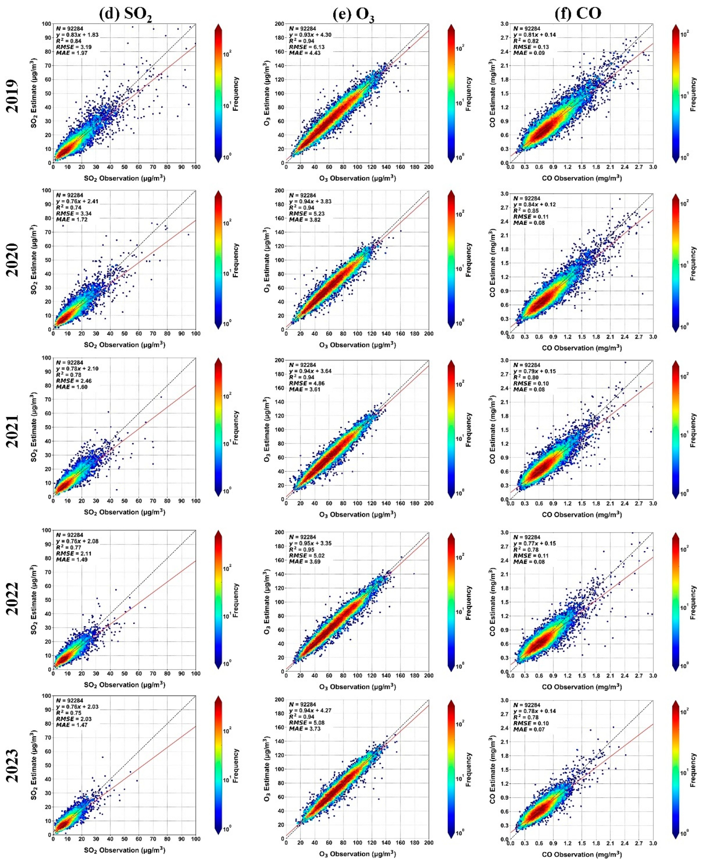
3.3.3. Spatial and Temporal Robustness of the Results
3.3.4. Comparisons of Multi-Output and Single-Output Models
4. Discussion
5. Conclusions
Author Contributions
Funding
Data Availability Statement
Acknowledgments
Conflicts of Interest
References
- Lelieveld, J.; Evans, J.S.; Fnais, M.; Giannadaki, D.; Pozzer, A. The Contribution of Outdoor Air Pollution Sources to Premature Mortality on a Global Scale. Nature 2015, 525, 367–371. [Google Scholar] [CrossRef]
- Zhou, X.; Zhang, X.; Wang, Y.; Chen, W.; Li, Q. Spatio-Temporal Variations and Socio-Economic Drivers of Air Pollution: Evidence from 332 Chinese Prefecture-Level Cities. Atmos. Pollut. Res. 2023, 14, 101782. [Google Scholar] [CrossRef]
- Landrigan, P.J. Air Pollution and Health. Lancet Public Health 2017, 2, e4–e5. [Google Scholar] [CrossRef]
- Brunekreef, B.; Holgate, S.T. Air Pollution and Health. Lancet 2002, 360, 1233–1242. [Google Scholar] [CrossRef]
- Silva, R.A.; West, J.J.; Lamarque, J.-F.; Shindell, D.T.; Collins, W.J.; Faluvegi, G.; Folberth, G.A.; Horowitz, L.W.; Nagashima, T.; Naik, V. Future Global Mortality from Changes in Air Pollution Attributable to Climate Change. Nat. Clim. Chang. 2017, 7, 647–651. [Google Scholar] [CrossRef]
- Cooper, M.J.; Martin, R.V.; Hammer, M.S.; Levelt, P.F.; Veefkind, P.; Lamsal, L.N.; Krotkov, N.A.; Brook, J.R.; McLinden, C.A. Global Fine-Scale Changes in Ambient NO2 during COVID-19 Lockdowns. Nature 2022, 601, 380–387. [Google Scholar] [CrossRef]
- Castells-Quintana, D.; Dienesch, E.; Krause, M. Air Pollution in an Urban World: A Global View on Density, Cities and Emissions. Ecol. Econ. 2021, 189, 107153. [Google Scholar] [CrossRef]
- Sicard, P.; Agathokleous, E.; Anenberg, S.C.; De Marco, A.; Paoletti, E.; Calatayud, V. Trends in Urban Air Pollution over the Last Two Decades: A Global Perspective. Sci. Total Environ. 2023, 858, 160064. [Google Scholar] [CrossRef]
- Rudke, A.P.; Martins, J.A.; Hallak, R.; Martins, L.D.; de Almeida, D.S.; Beal, A.; Freitas, E.D.; Andrade, M.F.; Koutrakis, P.; Albuquerque, T.T.A. Evaluating TROPOMI and MODIS Performance to Capture the Dynamic of Air Pollution in São Paulo State: A Case Study during the COVID-19 Outbreak. Remote Sens. Environ. 2023, 289, 113514. [Google Scholar] [CrossRef]
- Venter, Z.S.; Aunan, K.; Chowdhury, S.; Lelieveld, J. COVID-19 Lockdowns Cause Global Air Pollution Declines. Proc. Natl. Acad. Sci. USA 2020, 117, 18984–18990. [Google Scholar] [CrossRef]
- Fu, F.; Purvis-Roberts, K.L.; Williams, B. Impact of the COVID-19 Pandemic Lockdown on Air Pollution in 20 Major Cities around the World. Atmosphere 2020, 11, 1189. [Google Scholar] [CrossRef]
- Huang, Y.; Yang, S.; Zou, Y.; Su, J.; Wu, C.; Zhong, B.; Jia, P. Spatiotemporal Epidemiology of COVID-19 from an Epidemic Course Perspective. Geospat. Health 2022, 17. [Google Scholar] [CrossRef]
- Jia, P.; Yang, S. Are We Ready for a New Era of High-Impact and High-Frequency Epidemics? Nature 2020, 580, 321–322. [Google Scholar] [CrossRef]
- Burki, T. Dynamic Zero COVID Policy in the Fight against COVID. Lancet Respir. Med. 2022, 10, e58–e59. [Google Scholar] [CrossRef]
- Liu, Y.; Saltman, R.B. Policy Lessons from Early Reactions to the COVID-19 Virus in China. Am. J. Public Health 2020, 110, 1145–1148. [Google Scholar] [CrossRef]
- Pei, Z.; Han, G.; Ma, X.; Su, H.; Gong, W. Response of Major Air Pollutants to COVID-19 Lockdowns in China. Sci. Total Environ. 2020, 743, 140879. [Google Scholar] [CrossRef]
- Gao, C.; Zhang, F.; Fang, D.; Wang, Q.; Liu, M. Spatial Characteristics of Change Trends of Air Pollutants in Chinese Urban Areas during 2016–2020: The Impact of Air Pollution Controls and the COVID-19 Pandemic. Atmos. Res. 2023, 283, 106539. [Google Scholar] [CrossRef]
- Zhang, Q.; Mao, X.; Wang, Z.; Tan, Y.; Zhang, Z.; Wu, Y.; Gao, Y. Impact of the Emergency Response to COVID-19 on Air Quality and Its Policy Implications: Evidence from 290 Cities in China. Environ. Sci. Policy 2023, 145, 50–59. [Google Scholar] [CrossRef]
- Lv, Y.; Tian, H.; Luo, L.; Liu, S.; Bai, X.; Zhao, H.; Zhang, K.; Lin, S.; Zhao, S.; Guo, Z.; et al. Understanding and Revealing the Intrinsic Impacts of the COVID-19 Lockdown on Air Quality and Public Health in North China Using Machine Learning. Sci. Total Environ. 2023, 857, 159339. [Google Scholar] [CrossRef]
- Ma, Q.; Wang, J.; Xiong, M.; Zhu, L. Air Quality Index (AQI) Did Not Improve during the COVID-19 Lockdown in Shanghai, China, in 2022, Based on Ground and TROPOMI Observations. Remote Sens. 2023, 15, 1295. [Google Scholar] [CrossRef]
- Ministry of Ecology and Environment of the People’s Republic of China. Ambien Air Quality Standards (GB 3095-2012). 2012. Available online: https://www.mee.gov.cn/ywgz/fgbz/bz/bzwb/dqhjbh/dqhjzlbz/201203/t20120302_224165.shtml (accessed on 1 April 2024). (In Chinese)
- Wang, Z.; Tan, Y.; Guo, M.; Cheng, M.; Gu, Y.; Chen, S.; Wu, X.; Chai, F. Prospect of China’s Ambient Air Quality Standards. J. Environ. Sci. 2023, 123, 255–269. [Google Scholar] [CrossRef]
- Qin, W.; Fang, H.; Wang, L.; Wei, J.; Zhang, M.; Su, X.; Bilal, M.; Liang, X. MODIS High-Resolution MAIAC Aerosol Product: Global Validation and Analysis. Atmos. Environ. 2021, 264, 118684. [Google Scholar] [CrossRef]
- Veefkind, J.P.; Aben, I.; McMullan, K.; Förster, H.; De Vries, J.; Otter, G.; Claas, J.; Eskes, H.J.; De Haan, J.F.; Kleipool, Q. TROPOMI on the ESA Sentinel-5 Precursor: A GMES Mission for Global Observations of the Atmospheric Composition for Climate, Air Quality and Ozone Layer Applications. Remote Sens. Environ. 2012, 120, 70–83. [Google Scholar] [CrossRef]
- Wu, S.; Huang, B.; Wang, J.; He, L.; Wang, Z.; Yan, Z.; Lao, X.; Zhang, F.; Liu, R.; Du, Z. Spatiotemporal Mapping and Assessment of Daily Ground NO2 Concentrations in China Using High-Resolution TROPOMI Retrievals. Environ. Pollut. 2021, 273, 116456. [Google Scholar] [CrossRef]
- Kim, M.; Brunner, D.; Kuhlmann, G. Importance of Satellite Observations for High-Resolution Mapping of near-Surface NO2 by Machine Learning. Remote Sens. Environ. 2021, 264, 112573. [Google Scholar] [CrossRef]
- Goldberg, D.L.; Harkey, M.; de Foy, B.; Judd, L.; Johnson, J.; Yarwood, G.; Holloway, T. Evaluating NOx Emissions and Their Effect on O3 Production in Texas Using TROPOMI NO2 and HCHO. Atmos. Chem. Phys. 2022, 22, 10875–10900. [Google Scholar] [CrossRef]
- Hersbach, H.; Bell, B.; Berrisford, P.; Hirahara, S.; Horányi, A.; Muñoz-Sabater, J.; Nicolas, J.; Peubey, C.; Radu, R.; Schepers, D.; et al. The ERA5 Global Reanalysis. Q. J. R. Meteorol. Soc. 2020, 146, 1999–2049. [Google Scholar] [CrossRef]
- Zuo, C.; Chen, J.; Zhang, Y.; Jiang, Y.; Liu, M.; Liu, H.; Zhao, W.; Yan, X. Evaluation of Four Meteorological Reanalysis Datasets for Satellite-Based PM2.5 Retrieval over China. Atmos. Environ. 2023, 305, 119795. [Google Scholar] [CrossRef]
- Mu, X.; Wang, S.; Jiang, P.; Wang, B.; Wu, Y.; Zhu, L. Full-Coverage Spatiotemporal Estimation of Surface Ozone over China Based on a High-Efficiency Deep Learning Model. Int. J. Appl. Earth Obs. Geoinf. 2023, 118, 103284. [Google Scholar] [CrossRef]
- Jacquemin, B.; Lepeule, J.; Boudier, A.; Arnould, C.; Benmerad, M.; Chappaz, C.; Ferran, J.; Kauffmann, F.; Morelli, X.; Pin, I.; et al. Impact of Geocoding Methods on Associations between Long-Term Exposure to Urban Air Pollution and Lung Function. Environ. Health Perspect. 2013, 121, 1054–1060. [Google Scholar] [CrossRef]
- Wei, J.; Li, Z.; Cribb, M.; Huang, W.; Xue, W.; Sun, L.; Guo, J.; Peng, Y.; Li, J.; Lyapustin, A.; et al. Improved 1 Km Resolution PM2.5 Estimates across China Using Enhanced Space–Time Extremely Randomized Trees. Atmos. Chem. Phys. 2020, 20, 3273–3289. [Google Scholar] [CrossRef]
- Yang, N.; Shi, H.; Tang, H.; Yang, X. Geographical and Temporal Encoding for Improving the Estimation of PM2.5 Concentrations in China Using End-to-End Gradient Boosting. Remote Sens. Environ. 2022, 269, 112828. [Google Scholar] [CrossRef]
- Ke, G.; Meng, Q.; Finley, T.; Wang, T.; Chen, W.; Ma, W.; Ye, Q.; Liu, T.-Y. LightGBM: A Highly Efficient Gradient Boosting Decision Tree. In Proceedings of the Advances in Neural Information Processing Systems, Long Beach, CA, USA, 4–9 December 2017; Volume 30. [Google Scholar]
- Zhong, J.; Zhang, X.; Gui, K.; Wang, Y.; Che, H.; Shen, X.; Zhang, L.; Zhang, Y.; Sun, J.; Zhang, W. Robust Prediction of Hourly PM2.5 from Meteorological Data Using LightGBM. Natl. Sci. Rev. 2021, 8, nwaa307. [Google Scholar] [CrossRef]
- Ma, J.; Zhang, R.; Xu, J.; Yu, Z. MERRA-2 PM2. 5 Mass Concentration Reconstruction in China Mainland Based on LightGBM Machine Learning. Sci. Total Environ. 2022, 827, 154363. [Google Scholar] [CrossRef]
- Pedregosa, F.; Varoquaux, G.; Gramfort, A.; Michel, V.; Thirion, B.; Grisel, O.; Blondel, M.; Prettenhofer, P.; Weiss, R.; Dubourg, V. Scikit-Learn: Machine Learning in Python. J. Mach. Learn. Res. 2011, 12, 2825–2830. [Google Scholar]
- Yang, Q.; Kim, J.; Cho, Y.; Lee, W.-J.; Lee, D.-W.; Yuan, Q.; Wang, F.; Zhou, C.; Zhang, X.; Xiao, X.; et al. A Synchronized Estimation of Hourly Surface Concentrations of Six Criteria Air Pollutants with GEMS Data. NPJ Clim. Atmos. Sci. 2023, 6, 94. [Google Scholar] [CrossRef]
- Kohavi, R. A Study of Cross-Validation and Bootstrap for Accuracy Estimation and Model Selection. In Proceedings of the IJCAI, Montreal, QC, Canada, 20–25 August 1995; Volume 14, pp. 1137–1145. [Google Scholar]
- Fushiki, T. Estimation of Prediction Error by Using K-Fold Cross-Validation. Stat. Comput. 2011, 21, 137–146. [Google Scholar] [CrossRef]
- Esri. How Emerging Hot Spot Analysis Works. 2016. Available online: https://pro.arcgis.com/en/pro-app/3.1/tool-reference/space-time-pattern-mining/learnmoreemerging.htm (accessed on 1 April 2024).
- Ord, J.K.; Getis, A. Local Spatial Autocorrelation Statistics: Distributional Issues and an Application. Geogr. Anal. 1995, 27, 286–306. [Google Scholar] [CrossRef]
- Mann, H.B. Nonparametric Tests against Trend. Econom. J. Econom. Soc. 1945, 13, 245–259. [Google Scholar] [CrossRef]
- Kendall, M.G. Rank Correlation Methods; Griffin: Watertown, WI, USA, 1948. [Google Scholar]
- Thunis, P.; Clappier, A.; de Meij, A.; Pisoni, E.; Bessagnet, B.; Tarrason, L. Why Is the City’s Responsibility for Its Air Pollution Often Underestimated? A Focus on PM2.5. Atmos. Chem. Phys. 2021, 21, 18195–18212. [Google Scholar] [CrossRef]
- Friberg, M.D.; Zhai, X.; Holmes, H.A.; Chang, H.H.; Strickland, M.J.; Sarnat, S.E.; Tolbert, P.E.; Russell, A.G.; Mulholland, J.A. Method for Fusing Observational Data and Chemical Transport Model Simulations to Estimate Spatiotemporally Resolved Ambient Air Pollution. Environ. Sci. Technol. 2016, 50, 3695–3705. [Google Scholar] [CrossRef]
- Li, C.; Chen, Z.; Wang, X.; Wan, Y.; Zhao, Z. The Impact of COVID-19 on Economy, Air Pollution and Income: Evidence from China. Stoch. Environ. Res. Risk Assess. 2023, 37, 3343–3354. [Google Scholar] [CrossRef]
- Silva, A.C.T.; Branco, P.T.; Ferrini Rodrigues, P.; Sousa, S.I. Sustainable Policies for Air Pollution Reduction after COVID-19 Pandemic: Lessons Learnt from the Impact of the Different Lockdown Periods on Air Quality. Sustain. Dev. 2023, 31, 959–975. [Google Scholar] [CrossRef]
- Wang, R.; Peñuelas, J. Monitoring Compliance in Pandemic Management with Air Pollution Data: A Lesson from COVID-19. Environ. Sci. Technol. 2021, 55, 13571–13574. [Google Scholar] [CrossRef]
- Dong, L.; Chen, B.; Huang, Y.; Song, Z.; Yang, T. Analysis on the Characteristics of Air Pollution in China during the COVID-19 Outbreak. Atmosphere 2021, 12, 205. [Google Scholar] [CrossRef]
- Zhang, X.; Zhang, M.; Zhao, Z.; Huang, Z.; Deng, Q.; Li, Y.; Pan, A.; Li, C.; Chen, Z.; Zhou, M. Obesogenic Environmental Factors of Adult Obesity in China: A Nationally Representative Cross-Sectional Study. Environ. Res. Lett. 2020, 15, 044009. [Google Scholar] [CrossRef]
- Yang, S.; Liang, X.; Dou, Q.; La, Y.; Cai, J.; Yang, J.; Laba, C.; Liu, Q.; Guo, B.; Yu, W. Ethnic Disparities in the Association between Ambient Air Pollution and Risk for Cardiometabolic Abnormalities in China. Sci. Total Environ. 2022, 838, 155940. [Google Scholar] [CrossRef]
- Openshaw, S. The Modifiable Areal Unit Problem. In Concepts and Techniques in Modern Geography; Geo Books: Norwich, UK, 1984. [Google Scholar]
- Jia, P.; Yu, C.; Remais, J.V.; Stein, A.; Liu, Y.; Brownson, R.C.; Lakerveld, J.; Wu, T.; Yang, L.; Smith, M. Spatial Lifecourse Epidemiology Reporting Standards (ISLE-ReSt) Statement. Health Place 2020, 61, 102243. [Google Scholar] [CrossRef]
- Jia, P.; Stein, A. Using Remote Sensing Technology to Measure Environmental Determinants of Non-Communicable Diseases. Int. J. Epidemiol. 2017, 46, 1343–1344. [Google Scholar] [CrossRef] [PubMed]
- Chen, X.; Ye, X.; Widener, M.J.; Delmelle, E.; Kwan, M.-P.; Shannon, J.; Racine, E.F.; Adams, A.; Liang, L.; Jia, P. A Systematic Review of the Modifiable Areal Unit Problem (MAUP) in Community Food Environmental Research. Urban Inform. 2022, 1, 22. [Google Scholar] [CrossRef]
- Jia, P.; Stein, A.; James, P.; Brownson, R.C.; Wu, T.; Xiao, Q.; Wang, L.; Sabel, C.E.; Wang, Y. Earth Observation: Investigating Noncommunicable Diseases from Space. Annu. Rev. Public Health 2019, 40, 85–104. [Google Scholar] [CrossRef] [PubMed]
- Jia, P.; Liu, S.; Yang, S. Innovations in Public Health Surveillance for Emerging Infections. Annu. Rev. Public Health 2023, 44, 55–74. [Google Scholar] [CrossRef] [PubMed]


| Variable | Content | Unit | Spatial Resolution | Temporal Resolution | Data Source |
|---|---|---|---|---|---|
| Ground-based measurements | |||||
| PM2.5 | Ground-monitored PM2.5 concentration | µg/m3 | In situ | Hourly | China Environmental Monitoring Center |
| PM10 | Ground-monitored PM10 concentration | µg/m3 | |||
| O3 | Ground-monitored O3 concentration | µg/m3 | |||
| NO2 | Ground-monitored NO2 concentration | µg/m3 | |||
| SO2 | Ground-monitored SO2 concentration | µg/m3 | |||
| CO | Ground-monitored CO concentration | mg/m3 | |||
| Satellite-derived data | |||||
| AOD | Aerosol optical depth | – | 1 km × 1 km | Daily | Moderate-resolution Imaging Spectroradiometer (MODIS) |
| AAI | Absorbing aerosol index | – | 3.5 km × 7 km | Daily | Tropospheric Monitoring Instrument (TROPOMI) |
| TROPOMI CO | CO column number density | mol/m2 | |||
| TROPOMI NO2 | Tropospheric NO2 column number density | mol/m2 | |||
| TROPOMI O3 | O3 column number density | mol/m2 | |||
| Auxiliary data | |||||
| TEM | Temperature at 2 m | K | 0.1° × 0.1° | Monthly | European Centre for Medium-Range Weather Forecasts Reanalysis version 5 (ERA5) |
| DT | Dewpoint temperature at 2 m | K | |||
| WU | U-component of wind at 10 m | m/s | |||
| WV | V-component of wind at 10 m | m/s | |||
| SP | Surface pressure | hPa | |||
| ET | Total evaporation | mm | |||
| PRE | Total precipitation | mm | |||
| BLH | Boundary layer height | m | 0.25° × 0.25° | ||
| RH | Relative humidity | % | |||
| UVB | Downward UV radiation at the surface | J/m2 | |||
| SSR | Surface net solar radiation | J/m2 | |||
| STRD | Surface net thermal radiation | J/m2 | |||
| EI | Emission inventory | kt CO2/cell | 0.1° × 0.1° | Annual | Global Infrastructure Emissions Detector (GID) |
| NTL | Nighttime light | nW/sr/cm2 | 500 m × 500 m | Monthly | Visible Infrared Imaging Radiometer (VIIRS) |
| POP | Population counts | – | 1 km × 1 km | Annual | LandScan Global Population Data |
| NDVI | Normalized difference vegetation index | – | 1 km × 1 km | Monthly | Moderate-resolution Imaging Spectroradiometer (MODIS) |
| LUC | Land use cover | – | 1 km × 1 km | Annual | |
| DEM | Surface elevation | m | 90 m × 90 m | – | Shuttle Radar Topography Mission (SRTM) |
| Year | PM2.5 | PM10 | NO2 | SO2 | O3 | CO |
|---|---|---|---|---|---|---|
| 2019 | 29.7 ± 11.4 | 50.1 ± 24.6 | 12.2 ± 5.6 | 11.7 ± 2.0 | 70.5 ± 10.6 | 0.58 ± 0.17 |
| 2020 | 29.7 ± 11.0 | 49.0 ± 23.8 | 11.6 ± 5.0 | 11.7 ± 1.9 | 69.6 ± 10.6 | 0.58 ± 0.15 |
| 2021 | 28.4 ± 9.4 | 48.5 ± 22.5 | 11.7 ± 5.1 | 11.3 ± 1.9 | 70.4 ± 11.2 | 0.55 ± 0.15 |
| 2022 | 27.4 ± 9.5 | 47.7 ± 26.3 | 11.4 ± 4.5 | 10.6 ± 1.9 | 72.7 ± 11.0 | 0.51 ± 0.13 |
| 2023 | 28.7 ± 9.4 | 51.5 ± 25.5 | 11.9 ± 4.7 | 10.5 ± 1.9 | 73.1 ± 10.9 | 0.51 ± 0.14 |
| Sample-Based CV | Site-Based CV | Time-Based CV | |||||||
|---|---|---|---|---|---|---|---|---|---|
| R2 | RMSE | MAE | R2 | RMSE | MAE | R2 | RMSE | MAE | |
| PM2.5 | 0.92 | 6.11 | 3.09 | 0.90 | 6.91 | 3.66 | 0.82 | 9.17 | 5.27 |
| PM10 | 0.95 | 9.01 | 5.54 | 0.91 | 11.52 | 6.61 | 0.77 | 18.69 | 10.53 |
| NO2 | 0.90 | 3.79 | 2.80 | 0.90 | 3.96 | 2.95 | 0.85 | 4.75 | 3.56 |
| SO2 | 0.79 | 2.67 | 1.65 | 0.77 | 2.83 | 1.78 | 0.70 | 3.23 | 2.01 |
| O3 | 0.95 | 5.27 | 3.84 | 0.93 | 5.85 | 4.35 | 0.89 | 7.34 | 5.65 |
| CO | 0.82 | 0.11 | 0.08 | 0.79 | 0.12 | 0.09 | 0.73 | 0.14 | 0.10 |
| Sample-Based CV | Site-Based CV | Time-Based CV | |||||
|---|---|---|---|---|---|---|---|
| R2 | RMSE | R2 | RMSE | R2 | RMSE | ||
| PM2.5 | Multi-output | 0.92 | 6.11 | 0.90 | 6.91 | 0.82 | 9.17 |
| Single-output | 0.92 | 6.05 | 0.90 | 6.85 | 0.77 | 10.24 | |
| PM10 | Multi-output | 0.95 | 9.01 | 0.91 | 11.52 | 0.77 | 18.69 |
| Single-output | 0.94 | 9.15 | 0.91 | 11.56 | 0.76 | 19.13 | |
| NO2 | Multi-output | 0.90 | 3.79 | 0.90 | 3.96 | 0.85 | 4.75 |
| Single-output | 0.90 | 3.94 | 0.89 | 3.97 | 0.85 | 4.80 | |
| SO2 | Multi-output | 0.79 | 2.67 | 0.77 | 2.83 | 0.70 | 3.23 |
| Single-output | 0.78 | 2.75 | 0.77 | 2.83 | 0.69 | 3.25 | |
| O3 | Multi-output | 0.95 | 5.27 | 0.93 | 5.85 | 0.89 | 7.34 |
| Single-output | 0.95 | 5.28 | 0.93 | 5.81 | 0.89 | 7.48 | |
| CO | Multi-output | 0.82 | 0.11 | 0.79 | 0.12 | 0.73 | 0.14 |
| Single-output | 0.81 | 0.11 | 0.79 | 0.12 | 0.74 | 0.14 | |
Disclaimer/Publisher’s Note: The statements, opinions and data contained in all publications are solely those of the individual author(s) and contributor(s) and not of MDPI and/or the editor(s). MDPI and/or the editor(s) disclaim responsibility for any injury to people or property resulting from any ideas, methods, instructions or products referred to in the content. |
© 2024 by the authors. Licensee MDPI, Basel, Switzerland. This article is an open access article distributed under the terms and conditions of the Creative Commons Attribution (CC BY) license (https://creativecommons.org/licenses/by/4.0/).
Share and Cite
Qin, K.; Wang, Z.; Dai, S.; Li, Y.; Li, M.; Li, C.; Qiu, G.; Shi, Y.; Yin, C.; Yang, S.; et al. Spatiotemporal Patterns of Air Pollutants over the Epidemic Course: A National Study in China. Remote Sens. 2024, 16, 1298. https://doi.org/10.3390/rs16071298
Qin K, Wang Z, Dai S, Li Y, Li M, Li C, Qiu G, Shi Y, Yin C, Yang S, et al. Spatiotemporal Patterns of Air Pollutants over the Epidemic Course: A National Study in China. Remote Sensing. 2024; 16(7):1298. https://doi.org/10.3390/rs16071298
Chicago/Turabian StyleQin, Kun, Zhanpeng Wang, Shaoqing Dai, Yuchen Li, Manyao Li, Chen Li, Ge Qiu, Yuanyuan Shi, Chun Yin, Shujuan Yang, and et al. 2024. "Spatiotemporal Patterns of Air Pollutants over the Epidemic Course: A National Study in China" Remote Sensing 16, no. 7: 1298. https://doi.org/10.3390/rs16071298
APA StyleQin, K., Wang, Z., Dai, S., Li, Y., Li, M., Li, C., Qiu, G., Shi, Y., Yin, C., Yang, S., & Jia, P. (2024). Spatiotemporal Patterns of Air Pollutants over the Epidemic Course: A National Study in China. Remote Sensing, 16(7), 1298. https://doi.org/10.3390/rs16071298