Three-Dimensional Signal Source Localization with Angle-Only Measurements in Passive Sensor Networks

Abstract

Some passive sensors can provide only relative angles of a signal source. To obtain the signal source location, multiple passive sensors can be constructed into a passive sensor network through communication links. This paper investigates the source localization problem with angle-only measurements in three-dimensional space. First, we present an intersection localization method, which estimates the target position by minimizing the sum of distances between lines formed by angle-only measurements. It has the same target position estimate as the widely used least-squares (LS) method, but with a lower computational cost. Furthermore, considering the differences in measurement accuracy of sensors, the weighted least-squares (WLS) algorithm can achieve better localization performance than the LS method. Unfortunately, since the coefficient matrix and the noise vector are correlated, the WLS method is biased. The bias-compensation WLS (BCWLS) method is also presented in this paper to reduce the bias by estimating the correlation between the coefficient matrix and the pseudolinear noise vector. To evaluate the performance of the presented algorithms, numerical simulations are conducted, indicating that the superiority of the intersection localization method in computational cost and the superiority of the BCWLS method in localization accuracy.

1. Introduction

Signal source localization has applications in many fields, such as surveillance, guidance, and tracking [1,2,3]. In terms of whether to actively transmit electromagnetic signals, sensors for target localization can be divided into active sensors and passive sensors. Active sensors can achieve single-station positioning by transmitting signals to measure the distance to the target [4]. Passive sensors do not emit electromagnetic signals; therefore, they have a strong concealment [5]. Generally speaking, the types of passive sensors’ measurements include time delay (TD), Doppler shift (DS), angle of arrival (AOA), angle rate, or their combinations [6,7]. Among them, signal source localization with angle-only measurements has attracted considerable attention for many years, and it has been applied in many fields, including radar, sonar, navigation, and communications [8,9,10,11]. The signal source position cannot be obtained by the angle-only measurement in one snapshot with one passive sensor. Therefore, in order to estimate the signal source position, a widely used approach is to connect passive sensors distributed at different positions through communication links, and then design appropriate positioning algorithms to estimate the source position.

In the three-dimensional (3D) space, each passive sensor can measure the relative azimuth angle and elevation angle of the signal source, and output them as angle-only measurements. Therefore, it is obvious that each angle-only measurement can form a line with the sensor position as the endpoint. In the absence of noise, the signal source position are on a straight line, and the lines formed by the angle-only measurements of different sensors from the same signal source intersect at the signal source position. However, in practice, due to the presence of measurement error, including the angle measurement error and the sensor self-positioning error, even the lines formed by angle measurements from the same target are unlikely to intersect at the same point, but they intersect in a small volume. The small volume is determined by the level of the measurement noise. In [11], following this concept, a test statistic is constructed using the distance between the lines formed by angle-only measurements to complete the data association of angle-only measurements from different sensors.

Although the concept of target localization may be simple, it is challenging to obtain a robust and efficient estimate of the target position. Due to the nonlinearity of the signal source position and the angle-only measurement, signal source localization based on angle-only measurements is a nonlinear estimation problem [12,13]. To solve this problem, a pseudolinear equation regarding the signal source position is constructed by linearizing the angle measurement equation [6,8,10,14]. The least-squares (LS) method is an efficient and intuitive method to solve the pseudolinear overdetermined equation [15]. It is widely used because of its low complexity and stability. However, in the constructed pseudolinear overdetermined equation, the coefficient matrix is also contaminated by the measurement noise, which is not considered in the LS method [16,17]. The total least-squares (TLS) method not only considers the error of the data vector but also takes into account the perturbation of the coefficient matrix [18,19]. It is a natural generalization of the LS method [14,20]. In addition, the signal source position can also be estimated based on the spatial relationship between the source position and the lines formed by angle-only measurements [11,21,22,23].

The LS and TLS methods do not take into account the difference in the measurement noise levels of different sensors and they assume that the weights for different measurements are the same. Furthermore, to obtain a more accurate target position estimate, the weighted least-squares algorithm has been presented by considering the difference in measurement noise levels between different sensors [8,24]. The WLS algorithm is widely used due to its stability and accuracy [8,15,25,26]. Although the WLS method provides a more accurate target position estimate compared to the LS method, the WLS method is biased due to the presence of measurement noise not only in the pseudolinear noise vector but also in the coefficient matrix, especially if the angle measurement noise level is high [27]. To reduce the bias of the target position estimate, a series of methods have been investigated [28,29]. In 2D space, the bias-compensation operation is studied, which can reduce the bias to a certain extent [28]. In addition, from the perspective of reducing the noise of the coefficient matrix, the instrumental variables constructed in [29] can partly overcome the bias. Therefore, if the target is stationary or the observations of the sensors are synchronized, the above series of localization algorithms can be used to locate the target. However, if the target is moving and the sensor observations are not synchronized, it may be inappropriate to ignore the target movement.

To estimate the target motion state under asynchronous sensor observations, the gross LS method and the linear LS method are presented in [30]. In addition, a series of filtering algorithms have also been applied to estimate the target motion state with angle-only measurements [31]. Because of the nonlinearity of angle measurements and the target position, it is necessary to use a nonlinear tracking algorithm to estimate the target state. First, the standard Kalman filter algorithm has been used to process the pseudolinear equations constructed by the angle-only measurements, called pseudolinear Kalman filter (PLKF) [32,33]. In addition, many nonlinear filtering algorithms have also been used for target tracking with angle-only measurements. The extended Kalman filter (EKF) approximately obtains a linear observation equation through a first-order Taylor expansion. However, due to the neglect of high-order terms, it faces a filtering divergence problem when the measurement noise level is high [34]. Sigma-point Kalman filtering algorithms assume that approximating a distribution is easier than approximating a nonlinear function itself. They approximate the distribution of the target state by selecting a set of sigma points and use a Kalman filter to update the target state, such as the cubature Kalman filter (CKF) [35] or the unscented Kalman filter (UKF) [36,37]. In addition, the particle filter is also used for target tracking with angle-only measurement [38].

In this paper, we investigate the source localization problem with angle-only measurements from the passive sensor network connected by communication links in one snapshot. Firstly, we formulate an algorithm named intersection localization method, which is obtained by minimizing the distances between lines formed by the angle-only measurements. The LS method is also studied in this paper, which estimates the target position by solving the equation constructed using the angle measurements. By comparing the results of the presented intersection localization method and the LS method, we prove that the target position estimates of the intersection localization method and the LS method are the same. However, compared with the LS method, the coefficient matrix size of the proposed intersection localization method is smaller. Therefore, it requires smaller multiplication and addition operations. In theory, the computational cost of the intersection localization method is lower. Furthermore, the TLS method is studied, which takes into account not only errors in the data vector but also errors in the coefficient matrix. In practice, different sensors may have different levels of measurement noise. The WLS method is determined by considering the difference in measurement noise of different sensors. It is found that the WLS method is biased due to the presence of noise not only in the pseudolinear noise vector but also in the coefficient matrix. Therefore, we further formulate a bias-compensation WLS (BCWLS) algorithm by compensating the positioning bias of the WLS algorithm. To analyze the localization performance, the Cramér–Rao lower bound (CRLB) of the target position estimators based on angle-only measurements is also derived in this paper.

In numerical simulation, we analyze the impacts of angle measurement noise and sensor self-positioning noise on the target positioning accuracy of several algorithms. Numerical results show that the performance of the BCWLS method is closer to the CRLB performance among the above algorithms, proving the performance improvement of the BCWLS algorithm. In addition, it is verified that the intersection localization method and the LS method have the same target position estimate. Furthermore, we compare the running time of several algorithms under the same conditions, and the results verify the inference that the intersection localization algorithm requires a lower computational cost than the LS algorithm. Simulation results validate the performance of the proposed methods and demonstrate the improvement compared with the previous algorithms. In summary, the main contributions of this article can be highlighted as follows:

(1)

We present an intersection localization method with angle-only measurements in a passive sensor network. The presented intersection localization method has the same target position solution as the widely used and computationally efficient LS method but has a lower computational cost.

(2)

We present a bias computation WLS estimator for target localization using angle-only measurements. The presented method can compensate for the positioning bias of the WLS method, thereby improving the accuracy of the target position estimate.

(3)

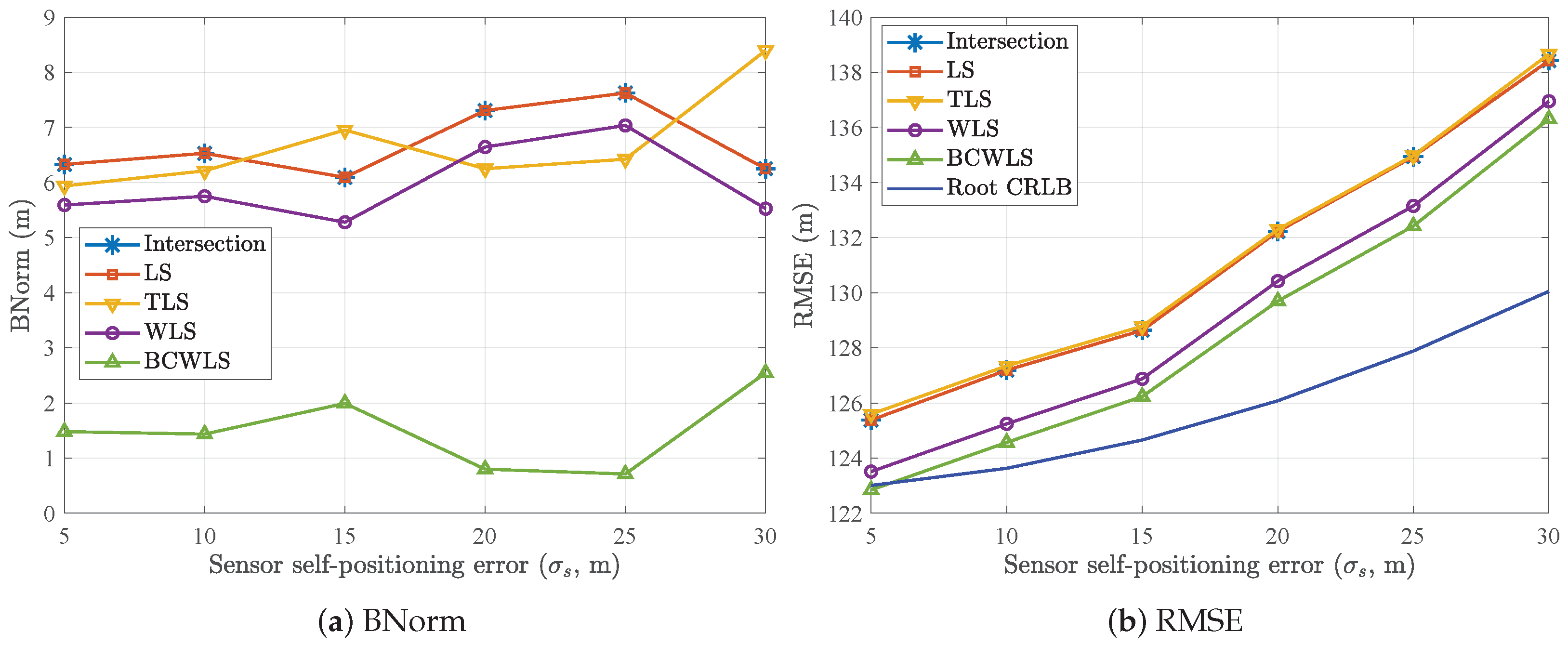
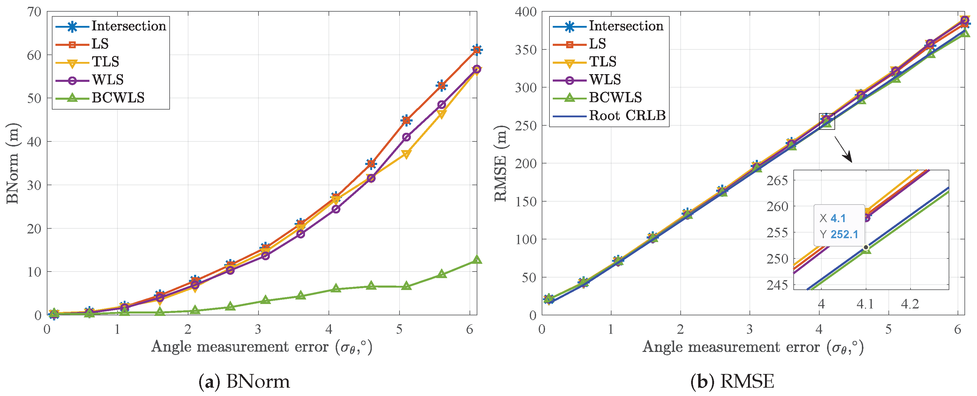
We derive the CRLB for estimating the target position under the condition of sensor self-positioning error. Numerical simulations evaluate the superiority of the intersection localization method in terms of computational cost and the superiority of the BCWLS method in terms of localization accuracy.

The rest of this article is sectioned as follows. In Section 2, we construct a target localization scenario with angle-only measurements in a passive sensor network and provide a series of target localization methods. In Section 2.2, we present an intersection localization method. In Section 2.3, Section 2.4 and Section 2.5, the LS, TLS, and WLS methods are introduced, respectively. In Section 2.6, we analyze the solution of the WLS method and further present a bias-compensation WLS method. Section 2.7 gives the CRLB of the target position estimators with angle-only measurements in passive sensor network. Section 3 examines the performance of the above methods via numerical simulations. Section 4 summarizes the results of the simulation results and provides the advantages and disadvantages of the two presented algorithms. Finally, Section 5 concludes this article.

2. Materials and Methods

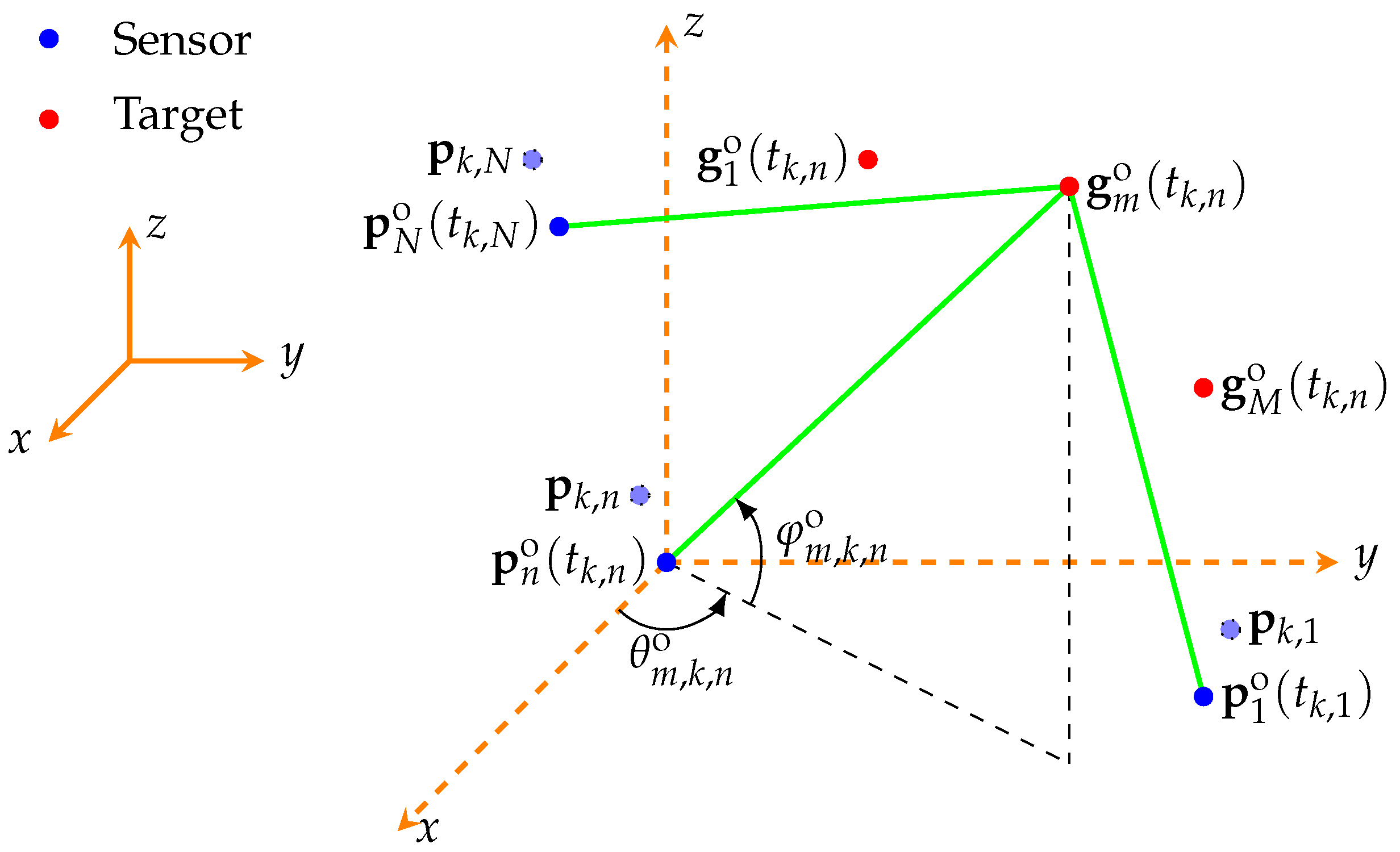
2.1. Signal Model of Angle-Only Measurements

We consider a 3D target localization scenario, which includes M targets and a passive sensor network. This passive sensor network consists of N passive sensors that can only provide the angle information of the target, such as passive radar, photoelectric sensor, and infrared sensor. In 3D space, angle-only measurements consist of azimuth and elevation angles. The true positions of the targets need to be estimated by the angle-only measurements. The position of each passive sensor is measured by its mounted positioning device, such as inertial navigation systems and the Global Positioning System (GPS). At time t, the true position of the nth sensor is denoted as ${\mathbf{p}}_n^{\mathrm{o}}\left(t\right)={[x_{n,s}^{\mathrm{o}}\left(t\right),y_{n,s}^{\mathrm{o}}\left(t\right),z_{n,s}^{\mathrm{o}}\left(t\right)]}^{\mathrm{T}}$, $n=1,2,\dots ,N$. The elements $x_{n,s}^{\mathrm{o}}\left(t\right)$, $y_{n,s}^{\mathrm{o}}\left(t\right)$ and $z_{n,s}^{\mathrm{o}}\left(t\right)$, respectively, represent the coordinates of the nth sensor on the x-axis, y-axis, and z-axis in the common coordinate system at time t. The notation ${[·]}^{\mathrm{T}}$ denotes the transpose operation. The true position of the mth target at time t is denoted as ${\mathbf{g}}_m^{\mathrm{o}}\left(t\right)={[x_{m,g}^{\mathrm{o}}\left(t\right),y_{m,g}^{\mathrm{o}}\left(t\right),z_{m,g}^{\mathrm{o}}\left(t\right)]}^{\mathrm{T}}$, $m=1,2,\dots ,M$. Figure 1 shows the 3D target localization scenario.

Assume that for the nth sensor, there are a total of $N_n$ observations. Each observation can receive radiation signals from multiple signal sources. The time instant of each observation can be defined as $t_{k,n}$, $k=1,\dots ,N_n$. For each radiation signal, the passive sensor can measure its AOA, termed angle-only measurement. At time instant $t_{k,n}$, the measurement of the nth sensor position can be expressed as

$$\begin{array}{c}\hfill {\mathbf{p}}_{k,n}\left(t_{k,n}\right)={\mathbf{p}}_n^{\mathrm{o}}\left(t_{k,n}\right)+\Delta {\mathbf{p}}_n\left(t_{k,n}\right)={[x_{n,s}\left(t_{k,n}\right),y_{n,s}\left(t_{k,n}\right),z_{n,s}\left(t_{k,n}\right)]}^{\mathrm{T}}\end{array}$$

(1)

where the vector $\Delta {\mathbf{p}}_n\left(t_{k,n}\right)$ is the sensor self-positioning noise. Without loss of generality, it is assumed to follow a zero-mean Gaussian distribution with the covariance matrix ${\mathbf{R}}_{s,n}\left(t_{k,n}\right)=\mathbb{E}(\Delta {\mathbf{p}}_n\left(t_{k,n}\right)\Delta {\mathbf{p}}_n^{\mathrm{T}}\left(t_{k,n}\right))$, namely $\Delta {\mathbf{p}}_n\left(t_{k,n}\right)\sim \mathcal{N}(\mathbf{0},{\mathbf{R}}_{s,n}\left(t_{k,n}\right))$. The notation $\mathbb{E}(·)$ is the expectation operation. At time instant $t_{k,n}$, the real position of the mth target can be denoted as

$${\mathbf{g}}_m^{\mathrm{o}}\left(t_{k,n}\right)={[x_{m,g}^{\mathrm{o}}\left(t_{k,n}\right),y_{m,g}^{\mathrm{o}}\left(t_{k,n}\right),z_{m,g}^{\mathrm{o}}\left(t_{k,n}\right)]}^{\mathrm{T}}.$$

(2)

Assuming that the nth sensor receives a total of $L_{k,n}$ signals corresponding to $L_{k,n}$ angle-only measurements during the kth observation. Therefore, the angle-only measurements of the kth observation of the nth sensor can be indexed by a triple $(l,k,n)$, $l=1,\dots ,L_{k,n}$. It should be noted that due to the presence of false alarms and missed detections, there may be a situation where $L_{k,n}$ is not equal to the number of targets M. In this way, we can establish a one-to-one index for all angle-only measurements of all sensors.

The set of angle-only measurements of the nth sensor at instant $t_{k,n}$ can be represented as ${\mathcal{L}}_{k,n}$, and

$$\begin{array}{c}\hfill {\mathcal{L}}_{k,n}=\left\{j\right|j=(l,k,n)\}.\end{array}$$

(3)

The cardinality of ${\mathcal{L}}_{k,n}$ satisfies $L_{k,n}=\left|{\mathcal{L}}_{k,n}\right|$, where the notation $|·|$ represents the cardinality of the set. Denote the set ${\mathcal{L}}_n$ and $\mathcal{L}$, which represent the set of measurements by the nth sensor and the set of measurements by N sensors, respectively. The sets ${\mathcal{L}}_n$ and $\mathcal{L}$ are

$$\begin{array}{c}\hfill {\mathcal{L}}_n={\cup }_{k=1}^{N_n}{\mathcal{L}}_{k,n},\mathcal{L}={\cup }_{n=1}^N{\mathcal{L}}_n\end{array}$$

(4)

where the notation ∪ represents the union operation. Therefore, we define $N_{\mathrm{s}}$ as the total number of the angle-only measurements of N sensors,

$$\begin{array}{c}\hfill N_{\mathrm{s}}=\left|\mathcal{L}\right|=\sum _{n=1}^N\sum _{k=1}^{N_n}{L}_{k,n}.\end{array}$$

(5)

It is necessary to associate the measurements of N sensors before target localization. Each angle-only measurement can only come from one of M targets or a false alarm. We define a set $\mathcal{M}=\{0,1,\dots ,M\}$ as the associated results’ index set, where the index 0 represents the false alarm, and the index $1,\dots ,M$ represent target $1,\cdots ,M$, respectively. Each angle-only measurement corresponds only to one member of the set $\mathcal{M}$. In our previous work [11], we constructed a test statistic using the minimum distance between the lines formed by the angle-only measurements of different sensors and then achieved the data association of the angle-only measurements. Then, we can obtain a mapping $\psi :\mathcal{L}\to \mathcal{M}$, which represents that any element in $\mathcal{L}$ corresponds to a unique element in $\mathcal{M}$. Therefore, after data association, the index set $\mathcal{L}$ can be divided into $M+1$ disjoint set, denoted as ${\mathcal{B}}_0,{\mathcal{B}}_1,\dots ,{\mathcal{B}}_M$, where ${\mathcal{B}}_0$ represents the index set of angle-only measurements from the false alarm, and ${\mathcal{B}}_m$ represents the index set of angle-only measurements from the mth target, where ${\mathcal{B}}_m$ is

$$\begin{array}{c}\hfill {\mathcal{B}}_m=\left\{j\right|\psi \left(j\right)=m,j\in \mathcal{L}\}\end{array}$$

(6)

where the sets ${\mathcal{B}}_i$ and ${\mathcal{B}}_j$ satisfy ${\mathcal{B}}_i\cap {\mathcal{B}}_j=\varnothing$, $i,j\in \mathcal{M}$, $i\ne j$. The notation ∩ represents the intersection operation of sets. In this paper, we study the target localization problem with angle-only measurements from multiple passive sensors. Therefore, for simplicity, we assume that the data association of angle-only measurements has been completed, and the mapping $\psi$ is known. For the mth target, its angle-only measurements index set is ${\mathcal{B}}_m$. We assume that $|{\mathcal{B}}_m|=L_m$. For the angle-only measurement index $n\in {\mathcal{B}}_m$, assuming that the sensor position measurement of its corresponding sensor can be expressed as

$$\begin{array}{c}\hfill {\mathbf{p}}_n={\mathbf{p}}_n^{\mathrm{o}}+\Delta {\mathbf{p}}_n\end{array}$$

(7)

where the vector ${\mathbf{p}}_n$ represents the sensor position measurement, the vector ${\mathbf{p}}_n^{\mathrm{o}}$ represents the true sensor position, and the vector $\Delta {\mathbf{p}}_n$ represents the sensor self-positioning noise assumed to be a zero-mean Gaussian distribution with covariance matrix ${\mathbf{R}}_{\mathbf{p},n}$.

The positions of the sensors with respect to the $L_m$ angle-only measurements can be expressed as

$$\begin{array}{c}\hfill \mathbf{p}={\mathbf{p}}^{\mathrm{o}}+\Delta \mathbf{p}\end{array}$$

(8)

where $\mathbf{p}={[{\mathbf{p}}_1^{\mathrm{T}},{\mathbf{p}}_2^{\mathrm{T}},\dots ,{\mathbf{p}}_{L_m}^{\mathrm{T}}]}^{\mathrm{T}}$, ${\mathbf{p}}^{\mathrm{o}}={[{\mathbf{p}}_1^{\mathrm{o}\mathrm{T}},{\mathbf{p}}_2^{\mathrm{o}\mathrm{T}},\dots ,{\mathbf{p}}_{L_m}^{\mathrm{o}\mathrm{T}}]}^{\mathrm{T}}$, and $\Delta \mathbf{p}={[\Delta {\mathbf{p}}_1^{\mathrm{o}\mathrm{T}},\Delta {\mathbf{p}}_2^{\mathrm{o}\mathrm{T}},\dots ,\Delta {\mathbf{p}}_{L_m}^{\mathrm{o}\mathrm{T}}]}^{\mathrm{T}}$. The covariance matrix of $\Delta \mathbf{p}$ is ${\mathbf{R}}_{\mathbf{p}}=\mathrm{blkdiag}({\mathbf{R}}_{\mathbf{p},1},{\mathbf{R}}_{\mathbf{p},2},\dots ,{\mathbf{R}}_{\mathbf{p},L_m})$, where the notation $\mathrm{blkdiag}({\mathbf{A}}_1,{\mathbf{A}}_2,\dots ,{\mathbf{A}}_N)$ represents the operation of constructing a block diagonal matrix with the matrices ${\mathbf{A}}_1,{\mathbf{A}}_2,\dots ,{\mathbf{A}}_N$.

The true value of the azimuth angle ${\theta }_n^{\mathrm{o}}$ and elevation angle ${\phi }_n^{\mathrm{o}}$ corresponding to the nth angle-only measurement can be expressed as [34]

$$\begin{array}{cc}\hfill {\theta }_n^{\mathrm{o}}& =f_{\theta }({\mathbf{g}}_m^{\mathrm{o}},{\mathbf{p}}_n^o)={tan}^{-1}\left(\frac{y_{m,g}^{\mathrm{o}}-y_{n,s}^{\mathrm{o}}}{x_{m,g}^{\mathrm{o}}-x_{n,s}^{\mathrm{o}}}\right)\hfill \end{array}$$

(9)

$$\begin{array}{cc}\hfill {\phi }_n^{\mathrm{o}}& =f_{\phi }({\mathbf{g}}_m^{\mathrm{o}},{\mathbf{p}}_n^o)={tan}^{-1}\frac{z_{m,g}^{\mathrm{o}}-z_{n,s}^{\mathrm{o}}}{\sqrt{{(x_{m,g}^{\mathrm{o}}-x_{n,s}^{\mathrm{o}})}^2+{(y_{m,g}^{\mathrm{o}}-y_{n,s}^{\mathrm{o}})}^2}}\hfill \end{array}$$

(10)

where ${\mathbf{g}}_m^{\mathrm{o}}={[x_{m,g}^{\mathrm{o}},y_{m,g}^{\mathrm{o}},z_{m,g}^{\mathrm{o}}]}^{\mathrm{T}}$ represents the target position, ${\theta }_n^o\in [-\pi ,\pi ]$, ${\phi }_n^o\in [-\frac{\pi }{2},\frac{\pi }{2}]$, and ${tan}^{-1}$ is the 4-quadrant arctangent function.

In practice, the angle-only measurements ${\theta }_n$ and ${\phi }_n$ can be expressed as

$$\begin{array}{cc}\hfill {\theta }_n& ={\theta }_n^{\mathrm{o}}+\Delta {\theta }_n=f_{\theta }({\mathbf{g}}_m^{\mathrm{o}},{\mathbf{p}}_n)+\Delta {\theta }_n\hfill \end{array}$$

(11)

$$\begin{array}{cc}\hfill {\phi }_n& ={\phi }_n^{\mathrm{o}}+\Delta {\theta }_n=f_{\phi }({\mathbf{g}}_m^{\mathrm{o}},{\mathbf{p}}_n)+\Delta {\phi }_n\hfill \end{array}$$

(12)

where the elements $\Delta {\theta }_n$ and $\Delta {\phi }_n$ represent the angle measurement noise, ${\theta }_n\in [-\pi ,\pi ]$, and ${\phi }_n\in [-\frac{\pi }{2},\frac{\pi }{2}]$. Without loss of generality, we assume that $\Delta {\theta }_n$ and $\Delta {\phi }_n$ are zero-mean Gaussian noises with variances ${\sigma }_{\Delta {\theta }_n}^2$ and ${\sigma }_{\Delta {\phi }_n}^2$, namely, $\Delta {\theta }_n\sim \mathcal{N}(0,{\sigma }_{\Delta {\theta }_n}^2)$ and $\Delta {\phi }_n\sim \mathcal{N}(0,{\sigma }_{\Delta {\phi }_n}^2)$, respectively.

From (11) and (12), due to the presence of sensor positioning error, (11) and (12) can be expressed as

$$\begin{array}{cc}\hfill {\theta }_n& ={\theta }_n^{\mathrm{o}}+e_{\theta ,n}+\Delta {\theta }_n={\theta }_n^{\mathrm{o}}+{\delta }_{\theta ,n}\hfill \end{array}$$

(13)

$$\begin{array}{cc}\hfill {\phi }_n& ={\phi }_n^{\mathrm{o}}+e_{\phi ,n}+\Delta {\phi }_n={\phi }_n^{\mathrm{o}}+{\delta }_{\phi ,n}\hfill \end{array}$$

(14)

where the elements $e_{\theta ,n}$ and $e_{\phi ,n}$ denote the measurement noise of the azimuth and elevation angles, respectively, caused by the sensor self-positioning error. They can be expressed as

$$\begin{array}{c}\hfill e_{\theta ,n}=\frac{\partial f_{\theta }({\mathbf{g}}_m^{\mathrm{o}},{\mathbf{p}}_n)}{\partial {\mathbf{p}}_n^{\mathrm{T}}}\Delta {\mathbf{p}}_n,e_{\phi ,n}=\frac{\partial f_{\phi }({\mathbf{g}}_m^{\mathrm{o}},{\mathbf{p}}_n)}{\partial {\mathbf{p}}_n^{\mathrm{T}}}\Delta {\mathbf{p}}_n.\end{array}$$

(15)

Therefore, the elements ${\delta }_{\theta ,n}$ and ${\delta }_{\phi ,n}$ represent the total measurement error of the azimuth angle and elevation angle, respectively. Assuming that the sensor self-positioning noise and the angle measurement noise are independent of each other, the variances of ${\delta }_{\theta ,n}$ and ${\delta }_{\phi ,n}$ are

$$\begin{array}{cc}\hfill {\sigma }_{\theta ,n}^2& ={\sigma }_{\Delta {\theta }_n}^2+{\mathbf{b}}_{\theta ,n}^{\mathrm{T}}{\mathbf{R}}_{\mathbf{p},n}{\mathbf{b}}_{\theta ,n}\hfill \end{array}$$

(16)

$$\begin{array}{cc}\hfill {\sigma }_{\phi ,n}^2& ={\sigma }_{\Delta {\phi }_n}^2+{\mathbf{b}}_{\phi ,n}^{\mathrm{T}}{\mathbf{R}}_{\mathbf{p},n}{\mathbf{b}}_{\phi ,n}\hfill \end{array}$$

(17)

where

$$\begin{array}{c}\hfill {\mathbf{b}}_{\theta ,n}=\frac{\partial f_{\theta }({\mathbf{g}}_m^{\mathrm{o}},{\mathbf{p}}_n)}{\partial {\mathbf{p}}_n},{\mathbf{b}}_{\phi ,n}=\frac{\partial f_{\phi }({\mathbf{g}}_m^{\mathrm{o}},{\mathbf{p}}_n)}{\partial {\mathbf{p}}_n}\end{array}$$

(18)

The nth angle-only measurement vector is ${\mathit{\theta }}_n={[{\theta }_n,{\phi }_n]}^{\mathrm{T}}$, and its corresponding measurement error vector is ${\mathit{\delta }}_{\mathit{\theta },n}={[{\delta }_{\theta ,n},{\delta }_{\phi ,n}]}^{\mathrm{T}}$. The covariance matrix of ${\mathit{\delta }}_{\mathit{\theta },n}$ is ${\mathbf{R}}_{\mathit{\theta },n}=\mathrm{diag}({\sigma }_{\theta ,n}^2,{\sigma }_{\phi ,n}^2)$, where the notation $\mathrm{diag}(a_1,a_2,\dots ,a_N)$ represents the operation of constructing a diagonal matrix using $a_1,a_2,\dots ,a_N$.

The angle-only measurement vector of the mth target is

$$\begin{array}{c}\hfill \mathit{\theta }={\mathit{\theta }}^{\mathrm{o}}+{\mathit{\delta }}_{\mathit{\theta }}\end{array}$$

(19)

where $\mathit{\theta }={[{\mathit{\theta }}_1^{\mathrm{T}},{\mathit{\theta }}_2^{\mathrm{T}},\dots ,{\mathit{\theta }}_{L_m}^{\mathrm{T}}]}^{\mathrm{T}}$, ${\mathit{\theta }}^{\mathrm{o}}={[{\mathit{\theta }}_1^{\mathrm{o}\mathrm{T}},{\mathit{\theta }}_2^{\mathrm{o}\mathrm{T}},\dots ,{\mathit{\theta }}_{L_m}^{\mathrm{o}\mathrm{T}}]}^{\mathrm{T}}$, and ${\mathit{\delta }}_{\mathit{\theta }}={[{\mathit{\delta }}_{\mathit{\theta },1}^{\mathrm{T}},{\mathit{\delta }}_{\mathit{\theta },2}^{\mathrm{T}},\dots ,{\mathit{\delta }}_{\mathit{\theta },L_m}^{\mathrm{T}}]}^{\mathrm{T}}$. The covariance matrix of ${\mathit{\delta }}_{\mathit{\theta }}$ is ${\mathbf{R}}_{\mathit{\theta }}=\mathrm{blkdiag}({\mathbf{R}}_{\mathit{\theta },1},{\mathbf{R}}_{\mathit{\theta },2},\dots ,{\mathbf{R}}_{\theta ,L_m})$.

2.2. Intersection Localization Method

It is obvious that each angle-only measurement of a passive sensor forms a line in 3D space with the sensor position as the endpoint. Under the condition that this measurement is not a false alarm, and there is no measurement noise, the target is on that line. With multiple angle-only measurements from different sensors, the target can be located. The line formed by the nth measurement can be expressed as

$$\begin{array}{c}\hfill L_n:{\mathbf{x}}_n={\mathbf{p}}_n+{\alpha }_n{\mathbf{e}}_n,{\alpha }_n\in \mathbb{R}\end{array}$$

(20)

where the element ${\alpha }_n$ is a distance parameter indicating the distance to ${\mathbf{p}}_n$, the vector ${\mathbf{e}}_n={[e_{n,x},e_{n,y},e_{n,z}]}^{\mathrm{T}}$ denotes the normalized direction vector, and

$$\begin{array}{c}\hfill {\mathbf{e}}_n={[cos\left({\theta }_n\right)cos\left({\phi }_n\right),sin\left({\theta }_n\right)cos\left({\phi }_n\right),sin\left({\phi }_n\right)]}^{\mathrm{T}}\end{array}$$

(21)

where $\parallel {\mathbf{e}}_n\parallel =1$, and the notation $\parallel ·\parallel$ over a vector denotes the ${\ell }_2$-norm.

In [11], the minimum distance between two lines is used to solve the distance parameters of the two lines. In this part, we extend the algorithm such that the distance parameters $\mathit{\alpha }={[{\alpha }_1,\dots ,{\alpha }_{L_m}]}^{\mathrm{T}}$ are solved as a whole.

For simplicity, assume that the elements in ${\mathcal{B}}_m$ can be expressed by ${\mathcal{B}}_m=\{1,\dots ,L_m\}$. The square of the Euclidean distance between two points on two lines $L_i$, $L_j$ is

$$\begin{array}{cc}\hfill d_{i,j}=& \parallel {\mathbf{p}}_j-{\mathbf{p}}_i+({\mathbf{e}}_i,{\mathbf{e}}_j){[-{\alpha }_i,{\alpha }_j]}^{\mathrm{T}}{\parallel }^2\hfill \\ \hfill =& \parallel \mathbf{P}{\mathbf{I}}_{i,j}\mathbf{1}+\mathbf{E}{\mathbf{I}}_{i,j}{\alpha \parallel }^2\hfill \\ \hfill =& {\alpha }^{\mathrm{T}}{\mathbf{I}}_{i,j}{\mathbf{E}}^{\mathrm{T}}\mathbf{E}{\mathbf{I}}_{i,j}\alpha +2{\alpha }^{\mathrm{T}}{\mathbf{I}}_{i,j}{\mathbf{E}}^{\mathrm{T}}\mathbf{P}{\mathbf{I}}_{i,j}\mathbf{1}+{\mathbf{1}}^{\mathrm{T}}{\mathbf{I}}_{i,j}{\mathbf{P}}^{\mathrm{T}}\mathbf{P}{\mathbf{I}}_{i,j}\mathbf{1}\hfill \end{array}$$

(22)

where $\mathbf{P}=[{\mathbf{p}}_1,\dots ,{\mathbf{p}}_{L_m}]\in {\mathbb{R}}^{3\times L_m}$, $\mathbf{E}=[{\mathbf{e}}_1,\dots ,{\mathbf{e}}_{L_m}]\in {\mathbb{R}}^{3\times L_m}$, the vector $\mathbf{1}\in {\mathbb{R}}^{L_m\times 1}$ denotes an all-one vector of length $L_m$, and the elements of matrix ${\mathbf{I}}_{i,j}\in {\mathbb{R}}^{L_m\times L_m}$ can be expressed as

$$\begin{array}{c}\hfill {\left[{\mathbf{I}}_{i,j}\right]}_{k,m}=\left\{\begin{array}{cc}1\hfill & k=m=j\hfill \\ -1\hfill & k=m=i\hfill \\ 0\hfill & \mathrm{else}.\hfill \end{array}\right.\end{array}$$

(23)

It should be noted that the distance $d_{i,j}$ is actually the square of the Euclidean distance, instead of the Euclidean distance itself. To extend the minimum total distance between all the lines, instead of two lines, we can formulate the optimization problem as

$$\begin{array}{c}\hfill \underset{\alpha }{min}d=\sum _{1\le i<j\le L_m}{d}_{i,j}\end{array}$$

(24)

where only one $(i,j)$ pair is taken into account in the summation operation since $d_{i,j}=d_{j,i}$.

It can be proved that the total distance can be expressed by

$$\begin{array}{c}\hfill d=\sum _{1\le i<j\le L_m}{d}_{i,j}={\mathit{\alpha }}^{\mathrm{T}}\mathbf{K}\mathit{\alpha }+2{\mathit{\alpha }}^{\mathrm{T}}\overline{\mathbf{K}}\mathbf{1}+{\mathbf{1}}^{\mathrm{T}}\tilde{\mathbf{K}}\mathbf{1}\end{array}$$

(25)

where

$$\begin{array}{cc}\hfill \mathbf{K}& =\sum _{1\le i<j\le L_m}{\mathbf{I}}_{i,j}{\mathbf{E}}^{\mathrm{T}}\mathbf{E}{\mathbf{I}}_{i,j}={\mathbf{K}}^{\mathrm{T}}\hfill \end{array}$$

(26)

$$\begin{array}{cc}\hfill \overline{\mathbf{K}}& =\sum _{1\le i<j\le L_m}{\mathbf{I}}_{i,j}{\mathbf{E}}^{\mathrm{T}}\mathbf{P}{\mathbf{I}}_{i,j}\hfill \end{array}$$

(27)

$$\begin{array}{cc}\hfill \tilde{\mathbf{K}}& =\sum _{1\le i<j\le L_m}{\mathbf{I}}_{i,j}{\mathbf{P}}^{\mathrm{T}}\mathbf{P}{\mathbf{I}}_{i,j}={\tilde{\mathbf{K}}}^{\mathrm{T}}.\hfill \end{array}$$

(28)

It is evident that $\mathbf{K}={\mathbf{K}}^{\mathrm{T}}$, and $\tilde{\mathbf{K}}={\tilde{\mathbf{K}}}^{\mathrm{T}}$. For any matrix $\mathbf{G}\in {\mathbb{R}}^{L_m\times L_m}$, we have

$${\left[{\mathbf{I}}_{i,j}\mathbf{G}{\mathbf{I}}_{i,j}\right]}_{k,m}=\left\{\begin{array}{cc}{G}_{i,i}\hfill & k=m=i\hfill \\ -G_{i,j}\hfill & k=i,m=j,\mathrm{or},k=j,m=i\hfill \\ G_{j,j}\hfill & k=m=j\hfill \\ 0\hfill & \mathrm{else}.\hfill \end{array}\right.$$

(29)

With this equation, we can verify that

$$\sum _{1\le i<j\le L_m}{\mathbf{I}}_{i,j}\mathbf{G}{\mathbf{I}}_{i,j}=L\mathrm{Diag}\left(\mathbf{G}\right)-\mathbf{G}$$

(30)

where the notation $\mathrm{Diag}(·)$ corresponds to a square matrix representing a diagonal matrix with the same diagonal elements as the input matrix.

Note that all the diagonal elements of $\mathbf{E}{\mathbf{E}}^{\mathrm{T}}$ are 1 since ${\mathbf{e}}^{\mathrm{T}}\mathbf{e}=1$; then,

$$\begin{array}{cc}\hfill \mathbf{K}& =\sum _{1\le i<j\le L_m}{\mathbf{I}}_{i,j}{\mathbf{E}}^{\mathrm{T}}\mathbf{E}{\mathbf{I}}_{i,j}=L_m\mathbf{I}-{\mathbf{E}}^{\mathrm{T}}\mathbf{E}\hfill \end{array}$$

(31)

$$\begin{array}{cc}\hfill \overline{\mathbf{K}}& =L_m\mathrm{Diag}\left({\mathbf{E}}^{\mathrm{T}}\mathbf{P}\right)-{\mathbf{E}}^{\mathrm{T}}\mathbf{P}\hfill \end{array}$$

(32)

$$\begin{array}{cc}\hfill \tilde{\mathbf{K}}& =L_m\mathrm{Diag}\left({\mathbf{P}}^{\mathrm{T}}\mathbf{P}\right)-{\mathbf{P}}^{\mathrm{T}}\mathbf{P}.\hfill \end{array}$$

(33)

To solve for the parameter $\mathit{\alpha }$ that minimizes d, we take the derivative of (25) with respect to $\mathit{\alpha }$,

$$\begin{array}{cc}\hfill \frac{\mathrm{d}d}{\mathrm{d}\mathit{\alpha }}& =2\mathbf{K}\mathit{\alpha }+2\overline{\mathbf{K}}\mathbf{1}.\hfill \end{array}$$

(34)

Setting (34) to zero and solving the equation, we obtain a solution

$$\frac{\mathrm{d}d}{\mathrm{d}\mathit{\alpha }}=0\Rightarrow {\mathit{\alpha }}_{\mathrm{opt}}=-{\mathbf{K}}^{-1}\overline{\mathbf{K}}\mathbf{1}$$

(35)

Putting ${\mathit{\alpha }}_{\mathrm{opt}}$ into (25), we obtain the minimal distance $d_{min}$ as

$$\begin{array}{c}\hfill d_{min}={\mathbf{1}}^{\mathrm{T}}(\tilde{\mathbf{K}}-\tilde{\mathbf{K}}{\mathbf{K}}^{-1}\tilde{\mathbf{K}})\mathbf{1}.\end{array}$$

(36)

In particular, if

$$\tilde{\mathbf{K}}=\tilde{\mathbf{K}}{\mathbf{K}}^{-1}\tilde{\mathbf{K}}$$

(37)

then

$$d_{min}=0.$$

(38)

In practice, the size of $\mathbf{K}$ is $L_m\times L_m$, and thus the computational cost to calculate ${\mathbf{K}}^{-1}$ is huge. According to the Sherman–Woodbury–Morrison equation,

$${(\mathbf{A}+\mathbf{B}\mathbf{C})}^{-1}={\mathbf{A}}^{-1}-{\mathbf{A}}^{-1}\mathbf{B}{(\mathbf{I}+\mathbf{C}{\mathbf{A}}^{-1}\mathbf{B})}^{-1}\mathbf{C}{\mathbf{A}}^{-1}$$

(39)

From $\mathbf{K}$ in (31), we let $\mathbf{A}\to -L_m\mathbf{I}$, $\mathbf{B}\to -{\mathbf{E}}^{\mathrm{T}}/L_m$, and $\mathbf{C}\to \mathbf{E}$; then, the matrix inversion operation ${\mathbf{K}}^{-1}$ can be simplified as

$${\mathbf{K}}^{-1}=\frac{1}{L_m}\mathbf{I}+\frac{1}{L_m^2}{\mathbf{E}}^{\mathrm{T}}{(\mathbf{I}-\mathbf{E}{\mathbf{E}}^{\mathrm{T}}/L_m)}^{-1}\mathbf{E}$$

(40)

where the only matrix inverse operation is over a $3\times 3$ matrix $\mathbf{I}-\mathbf{E}{\mathbf{E}}^{\mathrm{T}}/L_m$.

Consequently,

$$\begin{array}{c}\hfill \begin{array}{cc}\hfill {\mathbf{K}}^{-1}\overline{\mathbf{K}}& =\mathrm{Diag}\left({\mathbf{E}}^{\mathrm{T}}\mathbf{P}\right)-\frac{1}{L_m}{\mathbf{E}}^{\mathrm{T}}\mathbf{P}+\frac{1}{L_m^2}{\mathbf{E}}^{\mathrm{T}}{(\mathbf{I}-\mathbf{E}{\mathbf{E}}^{\mathrm{T}}/L_m)}^{-1}\mathbf{E}(L_m\mathrm{Diag}\left({\mathbf{E}}^{\mathrm{T}}\mathbf{P}\right)-{\mathbf{E}}^{\mathrm{T}}\mathbf{P})\hfill \\ \hfill & =\mathrm{Diag}\left({\mathbf{E}}^{\mathrm{T}}\mathbf{P}\right)-\frac{1}{L_m}{\mathbf{E}}^{\mathrm{T}}\mathbf{P}+\frac{1}{L_m}{\mathbf{E}}^{\mathrm{T}}{(\mathbf{I}-\mathbf{E}{\mathbf{E}}^{\mathrm{T}}/L_m)}^{-1}\mathbf{E}\mathrm{Diag}\left({\mathbf{E}}^{\mathrm{T}}\mathbf{P}\right)\hfill \\ \hfill & +\frac{1}{L_m}{\mathbf{E}}^{\mathrm{T}}{(\mathbf{I}-\mathbf{E}{\mathbf{E}}^{\mathrm{T}}/L_m)}^{-1}(\mathbf{I}-\mathbf{E}{\mathbf{E}}^{\mathrm{T}}/L_m-\mathbf{I})\mathbf{P}\hfill \\ \hfill & =\mathrm{Diag}\left({\mathbf{E}}^{\mathrm{T}}\mathbf{P}\right)+\frac{1}{L_m}{\mathbf{E}}^{\mathrm{T}}{(\mathbf{I}-\mathbf{E}{\mathbf{E}}^{\mathrm{T}}/L_m)}^{-1}(\mathbf{E}\mathrm{Diag}\left({\mathbf{E}}^{\mathrm{T}}\mathbf{P}\right)-\mathbf{P}).\hfill \end{array}\end{array}$$

(41)

The optimal weight can be written as

$${\mathit{\alpha }}_{\mathrm{opt}}=-{\mathbf{K}}^{-1}\overline{\mathbf{K}}\mathbf{1}=-\mathrm{diagvec}\left({\mathbf{E}}^{\mathrm{T}}\mathbf{P}\right)-\frac{1}{L_m}{\mathbf{E}}^{\mathrm{T}}{(\mathbf{I}-\mathbf{E}{\mathbf{E}}^{\mathrm{T}}/L_m)}^{-1}(\mathbf{E}\mathrm{diagvec}\left({\mathbf{E}}^{\mathrm{T}}\mathbf{P}\right)-\mathbf{P}\mathbf{1})$$

(42)

where the notation $\mathrm{diagvec}(·)$ with a square matrix input represents a vector formed by the diagonal elements of the input matrix.

For the ith line, the point corresponding to ${\alpha }_i$ is

$$\mathbf{x}\left(t_i\right)={\mathbf{p}}_i+{\alpha }_i{\mathbf{e}}_i$$

(43)

which, however, may be different for different lines. Therefore, we take the mean as the final estimate of the target position ${\mathbf{g}}_m^{\mathrm{o}}$, namely,

$$\begin{array}{c}\hfill \begin{array}{cc}\hfill {\widehat{\mathbf{g}}}_m& =\frac{1}{L_m}\sum _{i=1}^{L_m}\mathbf{x}\left(t_i\right)=\frac{1}{L_m}(\mathbf{P}\mathbf{1}+\mathbf{E}{\mathit{\alpha }}_{\mathrm{opt}})\hfill \\ \hfill & =\frac{1}{L_m}(\mathbf{P}\mathbf{1}-\mathbf{E}{\mathbf{K}}^{-1}\overline{\mathbf{K}}\mathbf{1})\hfill \\ \hfill & ={(L_m\mathbf{I}-\mathbf{E}{\mathbf{E}}^{\mathrm{T}})}^{-1}(\mathbf{P}\mathbf{1}-\mathbf{E}\mathrm{diagvec}\left({\mathbf{E}}^{\mathrm{T}}\mathbf{P}\right))\hfill \\ \hfill & ={(L_m\mathbf{I}-\mathbf{E}{\mathbf{E}}^{\mathrm{T}})}^{-1}\sum _{i=1}^{L_m}(\mathbf{I}-{\mathbf{e}}_i{\mathbf{e}}_i^{\mathrm{T}}){\mathbf{p}}_i.\hfill \end{array}\end{array}$$

(44)

2.3. Least-Squares Method

The LS method is a very classic and widely used method to solve linear overdetermined equations [15]. In this section, we use the LS method to solve the pseudolinear equations constructed by the angle measurement equations to estimate the target position. Firstly, let us derive the pseudolinear equations about a target position.

In (9), taking the tangent on both sides of the equation and replacing $tan{\theta }_n^{\mathrm{o}}$ with $sin{\theta }_n^{\mathrm{o}}/cos{\theta }_n^{\mathrm{o}}$, it can be rewritten as [8]

$$\begin{array}{c}\hfill {\mathbf{u}}_{\theta }^{\mathrm{o}\mathrm{T}}{\mathbf{p}}_n^{\mathrm{o}}={\mathbf{u}}_{\theta }^{\mathrm{o}\mathrm{T}}{\mathbf{g}}_m^{\mathrm{o}}\end{array}$$

(45)

where ${\mathbf{u}}_{\theta }^{\mathrm{o}}={[sin{\theta }_n^{\mathrm{o}},-cos{\theta }_n^{\mathrm{o}},0]}^{\mathrm{T}}$.

Replace ${\mathbf{p}}_n^{\mathrm{o}}$ and ${\mathit{\theta }}_n^o$ with their corresponding measurement values ${\mathbf{p}}_n$ and ${\mathit{\theta }}_n$, respectively. If the angle measurement noise is small, we have approximations of $sin{\delta }_{\theta ,n}\approx {\delta }_{\theta ,n}$ and $cos{\delta }_{\theta ,n}\approx 1$, then

$$\begin{array}{cc}\hfill sin{\theta }_n& =sin({\theta }_n^{\mathrm{o}}+{\delta }_{\theta ,n})\approx sin{\theta }_n^{\mathrm{o}}+{\delta }_{\theta ,n}cos{\theta }_n^{\mathrm{o}}\hfill \end{array}$$

(46)

$$\begin{array}{cc}\hfill cos{\theta }_n& =cos({\theta }_n^{\mathrm{o}}+{\delta }_{\theta ,n})\approx cos{\theta }_n^{\mathrm{o}}-{\delta }_{\theta ,n}sin{\theta }_n^{\mathrm{o}}.\hfill \end{array}$$

(47)

Taking (46) and (47) into (45), the pseudolinear equation obtained from the azimuth angle can be expressed as

$$\begin{array}{c}\hfill z_{\theta ,n}={\mathbf{A}}_{\theta ,n}{\mathbf{g}}_m^{\mathrm{o}}+{\eta }_{\theta ,n}\end{array}$$

(48)

where $z_{\theta ,n}={\mathbf{u}}_{\theta ,n}^{\mathrm{T}}{\mathbf{p}}_n$, ${\eta }_{\theta ,n}\approx -d_n^{\mathrm{o}}cos{\phi }_n^{\mathrm{o}}{\delta }_{\theta ,n}+{\mathbf{u}}_{\theta ,n}^{\mathrm{o}\mathrm{T}}\Delta {\mathbf{p}}_n$, ${\mathbf{A}}_{\theta ,n}={\mathbf{u}}_{\theta ,n}^{\mathrm{T}}$, ${\mathbf{u}}_{\theta ,n}={[sin{\theta }_n,-cos{\theta }_n,0]}^{\mathrm{T}}$, $d_n^{\mathrm{o}}=\parallel {\mathbf{p}}_n^{\mathrm{o}}-{\mathbf{g}}_m^{\mathrm{o}}\parallel$. In (48), we have used the geometric relationship $(x_{g,m}^{\mathrm{o}}-x_{n,s}^{\mathrm{o}})cos{\theta }_n^{\mathrm{o}}+(y_{g,m}^{\mathrm{o}}-y_{n,s}^{\mathrm{o}})sin{\theta }_n^{\mathrm{o}}=d_n^{\mathrm{o}}cos{\phi }_n^{\mathrm{o}}$.

Similarly, Equation (10) can be rewritten as [8]

$$\begin{array}{c}\hfill {\mathbf{u}}_{\phi ,n}^{\mathrm{o}\mathrm{T}}{\mathbf{p}}_n^{\mathrm{o}}={\mathbf{u}}_{\phi ,n}^{\mathrm{o}\mathrm{T}}{\mathbf{g}}_m^{\mathrm{o}}\end{array}$$

(49)

where ${\mathbf{u}}_{\phi ,n}^{\mathrm{o}}={[-cos{\theta }_n^{\mathrm{o}}sin{\phi }_n^{\mathrm{o}},-sin{\theta }_n^{\mathrm{o}}sin{\phi }_n^{\mathrm{o}},cos{\phi }_n^{\mathrm{o}}]}^{\mathrm{T}}$. Similarly, from (46) and (47), we also have the following approximation about the elevation angle

$$\begin{array}{cc}\hfill sin{\phi }_n& =sin({\phi }_n^{\mathrm{o}}+{\delta }_{\phi ,n})\approx sin{\phi }_n^{\mathrm{o}}+{\delta }_{\phi ,n}cos{\phi }_n^{\mathrm{o}}\hfill \end{array}$$

(50)

$$\begin{array}{cc}\hfill cos{\phi }_n& =cos({\phi }_n^{\mathrm{o}}+{\delta }_{\phi ,n})\approx cos{\phi }_n^{\mathrm{o}}-{\delta }_{\phi ,n}sin{\phi }_n^{\mathrm{o}}.\hfill \end{array}$$

(51)

Putting (46), (47), (50), (51), and the noisy sensor position ${\mathbf{p}}_n$ into (49), the pseudolinear equation obtained by the elevation angle can be expressed as

$$\begin{array}{c}\hfill z_{\phi ,n}={\mathbf{A}}_{\phi ,n}{\mathbf{g}}_m^{\mathrm{o}}+{\eta }_{\phi ,n}\end{array}$$

(52)

where $z_{\phi ,n}={\mathbf{u}}_{\phi ,n}^{\mathrm{T}}{\mathbf{p}}_n$, ${\mathbf{A}}_{\phi ,n}={\mathbf{u}}_{\phi ,n}^{\mathrm{T}}$, and ${\mathbf{u}}_{\phi ,n}={[-cos{\theta }_{n}sin{\phi }_n,-sin{\theta }_{n}sin{\phi }_n,cos{\phi }_n]}^{\mathrm{T}}$, ${\eta }_{\phi ,n}\approx d_n^{\mathrm{o}}{\delta }_{\phi ,n}+{\mathbf{u}}_{\phi ,n}^{\mathrm{o}\mathrm{T}}\Delta {\mathbf{p}}_n$. Combining (48) and (52) in matrix form, we obtain a pseudolinear equation,

$$\begin{array}{c}\hfill {\mathbf{z}}_n={\mathbf{A}}_n{\mathbf{g}}_m^{\mathrm{o}}+{\mathit{\eta }}_n\end{array}$$

(53)

where ${\mathbf{z}}_n={[z_{\theta ,n},z_{\phi ,n}]}^{\mathrm{T}}$, and ${\mathbf{A}}_n={[{\mathbf{u}}_{\theta ,n},{\mathbf{u}}_{\phi ,n}]}^{\mathrm{T}}\in {\mathbb{R}}^{2\times 3}$. The vector ${\mathit{\eta }}_n$ denotes the pseudolinear noise vector,

$$\begin{array}{c}\hfill {\mathit{\eta }}_n={[{\eta }_{\theta ,n},{\eta }_{\phi ,n}]}^{\mathrm{T}}\approx {\mathbf{D}}_n^{\mathrm{o}}{\delta }_{\theta ,n}+{\mathbf{A}}_n^{\mathrm{o}}\Delta {\mathbf{p}}_n\end{array}$$

(54)

where ${\mathbf{D}}_n^{\mathrm{o}}=\mathrm{diag}(-d_n^{\mathrm{o}}cos{\phi }_n^{\mathrm{o}},d_n^{\mathrm{o}})$ and ${\mathbf{A}}_n^{\mathrm{o}}={[{\mathbf{u}}_{\theta ,n}^{\mathrm{o}},{\mathbf{u}}_{\phi ,n}^{\mathrm{o}}]}^{\mathrm{T}}$. The covariance matrix of ${\mathit{\eta }}_n$ is

$$\begin{array}{c}\hfill {\mathbf{R}}_{\mathit{\eta },n}=\mathbb{E}[{\mathit{\eta }}_n,{\mathit{\eta }}_n^{\mathrm{T}}]={\mathbf{D}}_n^{\mathrm{o}}{\mathbf{R}}_{\theta ,n}{\mathbf{D}}_n^{\mathrm{o}\mathrm{T}}+{\mathbf{A}}_n^{\mathrm{o}}{\mathbf{R}}_{\mathbf{p},n}{\mathbf{A}}_n^{\mathrm{o}\mathrm{T}}.\end{array}$$

(55)

Combining (55) formed by $L_m$ angle-only measurements, we have

$$\begin{array}{c}\hfill \mathbf{z}=\mathbf{A}{\mathbf{g}}_m^{\mathrm{o}}+\mathit{\eta }\end{array}$$

(56)

where the coefficient matrix $\mathbf{A}$ and the data vector $\mathbf{z}$ can be expressed as

$$\begin{array}{cc}\hfill \mathbf{z}& ={[{\mathbf{z}}_1^{\mathrm{T}},{\mathbf{z}}_2^{\mathrm{T}},\dots ,{\mathbf{z}}_{L_m}^{\mathrm{T}}]}^{\mathrm{T}}\hfill \end{array}$$

(57)

$$\begin{array}{cc}\hfill \mathbf{A}& ={[{\mathbf{A}}_1^{\mathrm{T}},{\mathbf{A}}_2^{\mathrm{T}},\dots ,{\mathbf{A}}_{L_m}^{\mathrm{T}}]}^{\mathrm{T}}.\hfill \end{array}$$

(58)

The pseudolinear noise vector $\mathit{\eta }$ is

$$\begin{array}{c}\hfill \mathit{\eta }={[{\mathit{\eta }}_1^{\mathrm{T}},{\mathit{\eta }}_2^{\mathrm{T}},\dots ,{\mathit{\eta }}_{L_m}^{\mathrm{T}}]}^{\mathrm{T}}\approx {\mathbf{D}}^{\mathrm{o}}{\delta }_{\theta }+{\mathbf{B}}^{\mathrm{o}}\Delta \mathbf{p}\end{array}$$

(59)

where ${\mathbf{D}}^{\mathrm{o}}=\mathrm{blkdiag}({\mathbf{D}}_1^{\mathrm{o}},{\mathbf{D}}_2^{\mathrm{o}},\dots ,{\mathbf{D}}_{L_m}^{\mathrm{o}})$ and ${\mathbf{B}}^{\mathrm{o}}=\mathrm{blkdiag}({\mathbf{A}}_1^{\mathrm{o}},{\mathbf{A}}_2^{\mathrm{o}},\dots ,{\mathbf{A}}_{L_m}^{\mathrm{o}})$. The covariance matrix of vector $\mathit{\eta }$ can be expressed as

$$\begin{array}{c}\hfill {\mathbf{R}}_{\mathit{\eta }}=\mathrm{blkdiag}({\mathbf{R}}_{\mathit{\eta },1},{\mathbf{R}}_{\mathit{\eta },2},\dots ,{\mathbf{R}}_{\mathit{\eta },L_m}).\end{array}$$

(60)

With $L_m$ observations, there are a total of $2L_m$ equations about the target position ${\mathbf{g}}_m^{\mathrm{o}}$, and there are three unknown parameters in ${\mathbf{g}}_m^{\mathrm{o}}$. Therefore, if $L_m\ge 2$, ${\mathbf{g}}_m^{\mathrm{o}}$ has a solution, its LS solution can be obtained by minimizing $\parallel \mathit{\eta }\parallel$, which can be expressed as [15]

$$\begin{array}{c}\hfill {\widehat{\mathbf{g}}}_{m,\mathrm{LS}}={\left({\mathbf{A}}^{\mathrm{T}}\mathbf{A}\right)}^{-1}{\mathbf{A}}^{\mathrm{T}}\mathbf{z}.\end{array}$$

(61)

By rewriting the target position ${\mathbf{g}}_m^{\mathrm{o}}$ as ${\left({\mathbf{A}}^{\mathrm{T}}\mathbf{A}\right)}^{-1}{\mathbf{A}}^{\mathrm{T}}\mathbf{A}{\mathbf{g}}_m^{\mathrm{o}}$, the bias of the LS estimate ${\widehat{\mathbf{g}}}_{m,\mathrm{LS}}$ can be expressed as

$$\begin{array}{c}\hfill \mathbb{E}[\Delta {\mathbf{g}}_{m,LS}]=\mathbb{E}[{\mathbf{g}}_m^{\mathrm{o}}-{\widehat{\mathbf{g}}}_{m,\mathrm{LS}}]=-\mathbb{E}\left[{\left({\mathbf{A}}^{\mathrm{T}}\mathbf{A}\right)}^{-1}{\mathbf{A}}^{\mathrm{T}}\mathit{\eta }\right].\end{array}$$

(62)

We can see that if the measurement noise is negligible and the pseudolinear noise vector satisfies $\mathbb{E}\left[\mathit{\eta }\right]=\mathbf{0}$, the LS estimator can be seen as approximately unbiased.

It can be proved that the following equations exist

$$\begin{array}{cc}\hfill \mathbf{I}-{\mathbf{e}}_n{\mathbf{e}}_n^{\mathrm{T}}& ={\mathbf{A}}_n^{\mathrm{T}}{\mathbf{A}}_n\hfill \end{array}$$

(63)

$$\begin{array}{cc}\hfill {\mathbf{A}}_n^{\mathrm{T}}\mathbf{z}={\mathbf{A}}_n^{\mathrm{T}}{\mathbf{A}}_n{\mathbf{p}}_n& =(\mathbf{I}-{\mathbf{e}}_n{\mathbf{e}}_n^{\mathrm{T}}){\mathbf{p}}_n.\hfill \end{array}$$

(64)

Therefore, in (44) and (61), we have the following equations

$$\begin{array}{c}\hfill {(L_m\mathbf{I}-\mathbf{E}{\mathbf{E}}^{\mathrm{T}})}^{-1}=\left({\mathbf{A}}^{\mathrm{T}}\mathbf{A}\right)\end{array}$$

(65)

$$\begin{array}{c}\hfill \sum _{i=1}^{L_m}(\mathbf{I}-{\mathbf{e}}_i{\mathbf{e}}_i^{\mathrm{T}}){\mathbf{p}}_i={\mathbf{A}}^{\mathrm{T}}\mathbf{z}.\end{array}$$

(66)

Therefore, the target position estimate ${\widehat{\mathbf{g}}}_m$ of the intersection localization method and the LS estimate ${\widehat{\mathbf{g}}}_{m,LS}$ are equal. Due to the fact that the size of $\mathbf{A}$ in the LS method is $2L_m\times 3$, and the size of $\mathbf{E}$ in the intersection localization method is $3\times L_m$, their computational costs are different. In theory, the intersection localization method requires fewer multiplication and addition operations than the LS method.

2.4. Total Least-Squares Method

It should be noted that the construction of matrix $\mathbf{A}$ and vector $\mathbf{z}$ is based on the angle measurements and the sensor position measurements. Therefore, measurement noise not only exists in vector $\mathbf{z}$ but also in matrix $\mathbf{A}$, and Equation (56) can actually be expressed as [18]

$$\begin{array}{c}\hfill ({\mathbf{A}}^{\mathrm{o}}+\Delta \mathbf{A}){\mathbf{g}}_m^{\mathrm{o}}={\mathbf{z}}^{\mathrm{o}}+\Delta \mathbf{z}\end{array}$$

(67)

where $\mathbf{A}={\mathbf{A}}^{\mathrm{o}}+\Delta \mathbf{A}$, and $\mathbf{z}={\mathbf{z}}^{\mathrm{o}}+\Delta \mathbf{z}$. The matrix ${\mathbf{A}}^{\mathrm{o}}$ and the vector ${\mathbf{z}}^{\mathrm{o}}$ represent $\mathbf{A}$ and $\mathbf{z}$ with the noise values replaced by the true values, respectively.

By transferring items, (67) can be expressed as

$$\begin{array}{c}\hfill ({\mathbf{A}}^{\mathrm{o}}+\Delta \mathbf{A}|{\mathbf{z}}^{\mathrm{o}}+\Delta \mathbf{z})\left[\begin{array}{c}{\mathbf{g}}_m^{\mathrm{o}}\\ -1\end{array}\right]=\mathbf{0}.\end{array}$$

(68)

The TLS solution of the target position can be obtained by minimizing the Frobenius norm of the matrix $[\Delta \mathbf{A},\Delta \mathbf{z}]$. Therefore, the TLS estimate ${\widehat{\mathbf{g}}}_{m,\mathrm{TLS}}$ can be obtained by solving the following constrained optimization problem, as in [18],

$$\begin{array}{c}\hfill \begin{array}{cc}\hfill & \underset{{\widehat{\mathbf{g}}}_{m,\mathrm{TLS}},\Delta {\mathbf{A}}_{\mathrm{TLS}},\Delta {\mathbf{z}}_{\mathrm{TLS}}}{argmin}{\parallel \left[\begin{array}{cc}\Delta \mathbf{A}& \Delta \mathbf{z}\end{array}\right]\parallel }_{\mathrm{F}}\hfill \\ \hfill & \mathrm{s}.\mathrm{t}.(\mathbf{A}-\Delta \mathbf{A}){\mathbf{g}}_m^{\mathrm{o}}=\mathbf{z}-\Delta \mathbf{z}\hfill \end{array}\end{array}$$

(69)

where the notation ${\parallel ·\parallel }_{\mathrm{F}}$ with a matrix entry represents the Frobenius norm of the matrix. The TLS estimate ${\widehat{\mathbf{g}}}_{m,\mathrm{TLS}}$ of the target position ${\mathbf{g}}_m^{\mathrm{o}}$ can be obtained by singular value decomposition (SVD) of the augmented matrix $[\mathbf{A},-\mathbf{z}]$ [19].

Denote $\mathbf{C}=[\mathbf{A},-\mathbf{z}]\in {\mathbb{R}}^{2L_m\times 4}$, and the SVD of the matrix $\mathbf{C}$ is

$$\begin{array}{c}\hfill \mathbf{C}=\mathbf{U}\mathbf{\Sigma }{\mathbf{V}}^{\mathrm{T}}\end{array}$$

(70)

where the matrix $\mathbf{\Sigma }=\mathrm{diag}({\sigma }_1,\dots ,{\sigma }_4)$. ${\sigma }_1,\dots ,{\sigma }_4$ are the singular values of $\mathbf{C}$ and satisfy ${\sigma }_1\ge {\sigma }_2\dots \ge {\sigma }_4$. The matrix $\mathbf{V}$ can be partitioned as

$$\begin{array}{c}\hfill \mathbf{V}=\left[\begin{array}{cc}{\mathbf{V}}_{11}& {\mathbf{v}}_{12}\\ {\mathbf{v}}_{21}& v_{22}\end{array}\right]\end{array}$$

(71)

where ${\mathbf{V}}_{11}\in {\mathbb{R}}^{3\times 3}$, ${\mathbf{v}}_{12}\in {\mathbb{R}}^{3\times 1}$, ${\mathbf{v}}_{21}\in {\mathbb{R}}^{1\times 3}$, and $v_{22}\in {\mathbb{R}}^{1\times 1}$.

It has been proved in [19] that the TLS solution of (69) exists if and only if the element $v_{22}$ is non-singular, i.e., $v_{22}\ne 0$. In this case, the TLS estimate can be expressed as

$$\begin{array}{c}\hfill {\widehat{\mathbf{g}}}_{m,\mathrm{TLS}}={\mathbf{v}}_{12}{v}_{22}^{-1}.\end{array}$$

(72)

2.5. Weighted Least-Squares Method

The LS method applies the same weight to different measurements. However, in practice, the accuracy of different measurements may be different and may be known a priori. We assume that the distributions of angle-only measurement noise and sensor self-positioning noise are known a priori. Therefore, the target localization accuracy can be improved by giving proper weights to different measurements, which is the WLS method [8,14,15].

In (56), by considering the covariance of $\mathit{\eta }$, the cost function of the WLS formulation is

$$\begin{array}{c}\hfill J={(\mathbf{z}-\mathbf{A}{\mathbf{g}}_m^{\mathrm{o}})}^{\mathrm{T}}\mathbf{W}(\mathbf{z}-\mathbf{A}{\mathbf{g}}_m^{\mathrm{o}})\end{array}$$

(73)

where $\mathbf{W}$ is the weighting matrix,

$$\begin{array}{c}\hfill \mathbf{W}={\mathbf{R}}_{\mathit{\eta }}^{-1}=\mathrm{blkdiag}({\mathbf{W}}_1,{\mathbf{W}}_2,\dots ,{\mathbf{W}}_{L_m})\end{array}$$

(74)

where ${\mathbf{W}}_n={\mathbf{R}}_{\mathit{\eta },n}^{-1}$, $n=1,2,\dots ,L_m$.

The partial derivative of the cost function J for the target position ${\mathbf{g}}_m^{\mathrm{o}}$ is

$$\begin{array}{c}\hfill \frac{\partial J}{\partial {\mathbf{g}}_m^{\mathrm{o}}}=-2{\mathbf{A}}^{\mathrm{T}}\mathbf{W}\mathbf{z}+2{\mathbf{A}}^{\mathrm{T}}\mathbf{W}\mathbf{A}{\mathbf{g}}_m^{\mathrm{o}}.\end{array}$$

(75)

Let $\partial J/\partial {\mathbf{g}}_m^{\mathrm{o}}=0$; then, the WLS solution of the target position is [8]

$$\begin{array}{c}\hfill {\widehat{\mathbf{g}}}_{m,\mathrm{WLS}}={\left({\mathbf{A}}^{\mathrm{T}}\mathbf{W}\mathbf{A}\right)}^{-1}{\mathbf{A}}^{\mathrm{T}}\mathbf{W}\mathbf{z}.\end{array}$$

(76)

Rewriting the target position as ${\left({\mathbf{A}}^{\mathrm{T}}\mathbf{W}\mathbf{A}\right)}^{-1}{\mathbf{A}}^{\mathrm{T}}\mathbf{W}\mathbf{A}{\mathbf{g}}_m^{\mathrm{o}}$, we obtain the estimate error of ${\widehat{\mathbf{g}}}_{m,\mathrm{WLS}}$ as

$$\begin{array}{c}\hfill \Delta {\mathbf{g}}_{m,\mathrm{WLS}}={\widehat{\mathbf{g}}}_{m,\mathrm{WLS}}-{\mathbf{g}}_m^{\mathrm{o}}={\left({\mathbf{A}}^{\mathrm{T}}\mathbf{W}\mathbf{A}\right)}^{-1}{\mathbf{A}}^{\mathrm{T}}\mathbf{W}\mathit{\eta }.\end{array}$$

(77)

The covariance matrix of ${\widehat{\mathbf{g}}}_{m,\mathrm{WLS}}$ is [29]

$$\begin{array}{c}\hfill \begin{array}{cc}\hfill {\mathbf{R}}_{\mathbf{g},\mathrm{WLS}}& =\mathbb{E}[\Delta {\mathbf{g}}_{m,\mathrm{WLS}}\Delta {\mathbf{g}}_{m,\mathrm{WLS}}^{\mathrm{T}}]\hfill \\ \hfill & \approx {\left({\mathbf{A}}^{\mathrm{o}\mathrm{T}}\mathbf{W}{\mathbf{A}}^{\mathrm{o}}\right)}^{-1}{\mathbf{A}}^{\mathrm{o}\mathrm{T}}\mathbf{W}\mathbb{E}\left[\eta {\eta }^{\mathrm{T}}\right]{\mathbf{W}}^{\mathrm{T}}{\mathbf{A}}^{\mathrm{o}}{\left({\mathbf{A}}^{\mathrm{o}\mathrm{T}}\mathbf{W}{\mathbf{A}}^{\mathrm{o}}\right)}^{-1}={\left({\mathbf{A}}^{\mathrm{o}\mathrm{T}}\mathbf{W}{\mathbf{A}}^{\mathrm{o}}\right)}^{-1}\hfill \end{array}\end{array}$$

(78)

where we have used $\mathbb{E}\left[\mathit{\eta }{\mathit{\eta }}^{\mathrm{T}}\right]={\mathbf{W}}^{-1}$.

It should be noted that the weighting matrix $\mathbf{W}$ requires the unknown true position of the target via ${\mathbf{D}}^{\mathrm{o}}$ and ${\mathbf{B}}^{\mathrm{o}}$. To solve this problem, we obtain an initial target position estimate by using the LS method. The weighting matrix $\mathbf{W}$ can be obtained by this initial solution; then, the WLS estimate can be derived by (76).

2.6. Bias-Compensation WLS Method

This section firstly analyzes the bias issue of the WLS method introduced in Section 2.5. Then, a bias-compensated WLS method is studied by estimating the bias of the WLS estimate ${\widehat{\mathbf{g}}}_{m,\mathrm{WLS}}$.

The expectation of $\Delta {\mathbf{g}}_{m,\mathrm{WLS}}$ in (77) can be expressed as

$$\begin{array}{c}\hfill {\delta }_{\mathbf{g},\mathrm{WLS}}=\mathbb{E}[\Delta {\mathbf{g}}_{m,\mathrm{WLS}}]=\mathbb{E}\left[{\left({\mathbf{A}}^{\mathrm{T}}\mathbf{W}\mathbf{A}\right)}^{-1}{\mathbf{A}}^{\mathrm{T}}\mathbf{W}\mathit{\eta }\right]\approx {\left({\mathbf{A}}^{\mathrm{T}}\mathbf{W}\mathbf{A}\right)}^{-1}\mathbb{E}\left[{\mathbf{A}}^{\mathrm{T}}\mathbf{W}\mathit{\eta }\right]\end{array}$$

(79)

Since both the matrix $\mathbf{A}$ and the pseudolinear noise vector $\mathit{\eta }$ contain measurement noise, the matrix $\mathbf{A}$ and the noise vector $\mathit{\eta }$ are correlated. Therefore, $\mathbb{E}\left[{\mathbf{A}}^{\mathrm{T}}\mathbf{W}\mathit{\eta }\right]\ne \mathbf{0}$, so that the WLS estimator is biased.

Since the matrix $\mathbf{W}$ is a block diagonal matrix, the expectation $\mathbb{E}\left[{\mathbf{A}}^{\mathrm{T}}\mathbf{W}\mathit{\eta }\right]$ can be rewritten as

$$\begin{array}{c}\hfill \mathbb{E}\left[{\mathbf{A}}^{\mathrm{T}}\mathbf{W}\mathit{\eta }\right]=\sum _{n=1}^{L_m}\mathbb{E}\left[{\mathbf{A}}_n^{\mathrm{T}}{\mathbf{W}}_n{\mathit{\eta }}_n\right]\approx \sum _{n=1}^{L_m}{\mathbf{m}}_n.\end{array}$$

(80)

Because the weighting matrix ${\mathbf{W}}_n$ is the inverse of the covariance matrix ${\mathbf{R}}_n$, it is a symmetric matrix that can be expressed as

$$\begin{array}{c}\hfill {\mathbf{W}}_n=\left[\begin{array}{cc}{a}_n& b_n\\ b_n& c_n\end{array}\right]\end{array}$$

(81)

Putting (81) into (80), the vector ${\mathbf{m}}_n$ can be written as

$$\begin{array}{c}\hfill {\mathbf{m}}_n={\mathbf{g}}_{1,n}+{\mathbf{g}}_{2,n}\end{array}$$

(82)

where

$$\begin{array}{cc}\hfill {\mathbf{g}}_{1,n}& =\left(a_n{\mathbf{a}}_{1,n}{\mathbf{b}}_{\theta ,n}^{\mathrm{T}}+b_n({\mathbf{a}}_{2,n}{\mathbf{b}}_{\theta ,n}^{\mathrm{T}}+{\mathbf{a}}_{3,n}{\mathbf{b}}_{\phi ,n}^{\mathrm{T}})\right){\mathbf{R}}_{\mathbf{p},n}{\mathbf{u}}_{\theta ,n}^o-d_n^{o}cos{\phi }_n^o{\sigma }_{\Delta {\theta }_n}^2(a_n{\mathbf{a}}_{1,n}+b_n{\mathbf{a}}_{2,n})\hfill \end{array}$$

(83)

$$\begin{array}{cc}\hfill {\mathbf{g}}_{2,n}& =\left(b_n{\mathbf{a}}_{1,n}{\mathbf{b}}_{\theta ,n}^{\mathrm{T}}+c_n({\mathbf{a}}_{2,n}{\mathbf{b}}_{\theta ,n}^{\mathrm{T}}+{\mathbf{a}}_{3,n}{\mathbf{b}}_{\phi ,n}^{\mathrm{T}})\right){\mathbf{R}}_{\mathbf{p},n}{\mathbf{u}}_{\phi ,n}^o+c_n{d}_n^o{\mathbf{a}}_{3,n}{\sigma }_{\Delta {\phi }_n}^2\hfill \end{array}$$

(84)

where

$$\begin{array}{cc}\hfill {\mathbf{a}}_{1,n}& ={[cos{\theta }_n^{\mathrm{o}},sin{\theta }_n^{\mathrm{o}},0]}^{\mathrm{T}}\hfill \end{array}$$

(85)

$$\begin{array}{cc}\hfill {\mathbf{a}}_{2,n}& ={[sin{\theta }_n^{\mathrm{o}}sin{\phi }_n^{\mathrm{o}},-cos{\theta }_n^{\mathrm{o}}sin{\phi }_n^{\mathrm{o}},0]}^{\mathrm{T}}\hfill \end{array}$$

(86)

$$\begin{array}{cc}\hfill {\mathbf{a}}_{3,n}& =-{[cos{\theta }_n^{\mathrm{o}}cos{\phi }_n^{\mathrm{o}},sin{\theta }_n^{\mathrm{o}}cos{\phi }_n^{\mathrm{o}},sin{\phi }_n^{\mathrm{o}}]}^{\mathrm{T}}\hfill \end{array}$$

(87)

Therefore, according to (77), the bias-compensation WLS estimate of the target position is

$$\begin{array}{c}\hfill {\widehat{\mathbf{g}}}_{m,WLS}^{bc}={\widehat{\mathbf{g}}}_{m,WLS}-{\delta }_{\mathbf{g},WLS}.\end{array}$$

(88)

It should be noted that the calculation of ${\mathit{\delta }}_{\mathbf{g},WLS}$ depends on the true azimuth angle ${\theta }_n^{\mathrm{o}}$, elevation angle ${\phi }_n^{\mathrm{o}}$, and distance $d_n^{\mathrm{o}}$. To ensure accuracy, we can use the WLS solution ${\widehat{\mathbf{g}}}_{m,WLS}$ of the target position to estimate ${\mathit{\delta }}_{\mathbf{g},WLS}$ and then derive the final solution by (88).

2.7. Cramér–Rao Lower Bound

It is well-known that the CRLB establishes a lower bound on the performance of estimators [8,14,24]. Therefore, it is widely used to calculate the best estimation accuracy in theory and evaluate the performance of estimators. For the scenario in this article, with the presence of the sensor self-positioning noise, the unknown parameters include the target position ${\mathbf{g}}_m$ and the positions of the sensors ${\mathbf{p}}^{\mathrm{o}}$. Therefore, under the assumption that the angle-only measurements’ noise and the sensor self-positioning noise are independent and all subject to the zero-mean Gaussian distribution, we would like to derive the CRLB of the parameter vector $\mathbf{\Theta }={[{\mathbf{g}}_m^{\mathrm{o}\mathrm{T}},{\mathbf{p}}^{\mathrm{o}\mathrm{T}}]}^{\mathrm{T}}\in {\mathbb{R}}^{(3L_m+3)\times 1}$. The measurement vector consists of $L_m$ angle-only measurements $\mathit{\theta }$ and corresponding position measurements $\mathbf{p}$ of sensors, denoted by $\mathbf{m}={[{\mathit{\theta }}^{\mathrm{T}},{\mathbf{p}}^{\mathrm{T}}]}^{\mathrm{T}}\in {\mathbb{R}}^{5L_m\times 1}$. Under the given parameters $\mathbf{\Theta }$, the logarithm of the joint probability density function of $\mathbf{m}$ is

$$\begin{array}{cc}\hfill lnp\left(\mathbf{m}\right|\mathbf{\Theta })& =lnp\left(\mathit{\theta }\right|\mathbf{\Theta })+lnp(\mathbf{p}|\mathbf{\Theta })\hfill \\ \hfill & =\kappa -\frac{1}{2}{(\mathit{\theta }-{\mathit{\theta }}^{\mathrm{o}})}^{\mathrm{T}}{\mathbf{R}}_{\mathit{\theta }}^{-1}(\mathit{\theta }-{\mathit{\theta }}^{\mathrm{o}})-\frac{1}{2}{(\mathbf{p}-{\mathbf{p}}^{\mathrm{o}})}^{\mathrm{T}}{\mathbf{R}}_{\mathbf{p}}^{-1}(\mathbf{p}-{\mathbf{p}}^{\mathrm{o}})\hfill \end{array}$$

(89)

where $\kappa$ is a constant.

According to (89), the Fisher information matrix (FIM) of $\mathbf{\Theta }$ is

$$\begin{array}{c}\hfill \mathrm{FIM}(\mathbf{\Theta })=-E\left[\frac{\partial l{n}^{2}p\left(\mathbf{m}\right|\mathbf{\Theta })}{\partial \mathbf{\Theta }\partial {\mathbf{\Theta }}^{\mathrm{T}}}\right]\end{array}$$

(90)

The CRLB matrix of an estimate of $\mathbf{\Theta }$ is the inverse of $\mathrm{FIM}(\mathbf{\Theta })$:

$$\begin{array}{cc}\hfill \mathrm{CRLB}(\mathbf{\Theta })& ={\mathrm{FIM}}^{-1}(\mathbf{\Theta })\hfill \\ \hfill & ={\left[\begin{array}{cc}{\left[\frac{\partial {\mathit{\theta }}^{\mathrm{o}}}{\partial {\mathbf{g}}_m^{\mathrm{o}}}\right]}^{\mathrm{T}}{\mathbf{R}}_{\mathit{\theta }}^{-1}\frac{\partial {\mathit{\theta }}^{\mathrm{o}}}{\partial {\mathbf{g}}_m^{\mathrm{o}}}& {\left[\frac{\partial {\mathit{\theta }}^{\mathrm{o}}}{\partial {\mathbf{g}}_m^{\mathrm{o}}}\right]}^{\mathrm{T}}{\mathbf{R}}_{\mathit{\theta }}^{-1}\frac{\partial {\mathit{\theta }}^{\mathrm{o}}}{\partial {\mathbf{p}}^{\mathrm{o}}}\\ {\left[\frac{\partial {\mathit{\theta }}^{\mathrm{o}}}{\partial {\mathbf{p}}^{\mathrm{o}}}\right]}^{\mathrm{T}}{\mathbf{R}}_{\mathit{\theta }}^{-1}\frac{\partial {\mathit{\theta }}^{\mathrm{o}}}{\partial {\mathbf{g}}_m^{\mathrm{o}}}& {\left[\frac{\partial {\mathit{\theta }}^{\mathrm{o}}}{\partial {\mathbf{p}}^{\mathrm{o}}}\right]}^{\mathrm{T}}{\mathbf{R}}_{\mathit{\theta }}^{-1}\frac{\partial {\mathit{\theta }}^{\mathrm{o}}}{\partial {\mathbf{p}}^{\mathrm{o}}}+{\mathbf{R}}_{\mathbf{p}}^{-1}\end{array}\right]}^{-1}={\left[\begin{array}{cc}\mathbf{X}& \mathbf{Z}\\ {\mathbf{Z}}^{\mathrm{T}}& \mathbf{Y}\end{array}\right]}^{-1}\hfill \end{array}$$

(91)

where

$$\begin{array}{cc}\hfill \frac{\partial {\mathit{\theta }}^{\mathrm{o}}}{\partial {\mathbf{g}}_m^{\mathrm{o}}}& =\mathrm{blkdiag}\left(\frac{\partial {\mathit{\theta }}_1^{\mathrm{o}}}{\partial {\mathbf{g}}_m^{\mathrm{o}}},\frac{\partial {\mathit{\theta }}_2^{\mathrm{o}}}{\partial {\mathbf{g}}_m^{\mathrm{o}}},\dots ,\frac{\partial {\mathit{\theta }}_{L_m}^{\mathrm{o}}}{\partial {\mathbf{g}}_m^{\mathrm{o}}}\right)=\mathrm{blkdiag}({\mathbf{B}}_1,{\mathbf{B}}_2,\dots ,{\mathbf{B}}_{L_m})\in {\mathbb{R}}^{3L_m\times 2L_m}\hfill \end{array}$$

(92)

$$\begin{array}{cc}\hfill \frac{\partial {\mathit{\theta }}^{\mathrm{o}}}{\partial {\mathbf{p}}^{\mathrm{o}}}& =\mathrm{blkdiag}\left(\frac{\partial {\mathit{\theta }}_1^{\mathrm{o}}}{\partial {\mathbf{p}}_1^{\mathrm{o}}},\frac{\partial {\mathit{\theta }}_2^{\mathrm{o}}}{\partial {\mathbf{p}}_2^{\mathrm{o}}},\dots ,\frac{\partial {\mathit{\theta }}_{L_m}^{\mathrm{o}}}{\partial {\mathbf{p}}_{L_m}^{\mathrm{o}}}\right)=-\mathrm{blkdiag}({\mathbf{B}}_1,{\mathbf{B}}_2,\dots ,{\mathbf{B}}_{L_m})\in {\mathbb{R}}^{3L_m\times 2L_m}\hfill \end{array}$$

(93)

where

$$\begin{array}{cc}\hfill {\mathbf{B}}_n& =\frac{\partial {\mathit{\theta }}_n^{\mathrm{o}}}{\partial {\mathbf{g}}_m^{\mathrm{o}}}=\left[\frac{\partial {\theta }_n^{\mathrm{o}}}{\partial {\mathbf{g}}_m^{\mathrm{o}}},\frac{\partial {\phi }_n^{\mathrm{o}}}{\partial {\mathbf{g}}_m^{\mathrm{o}}}\right]\hfill \end{array}$$

(94)

$$\begin{array}{cc}\hfill \frac{\partial {\theta }_n^{\mathrm{o}}}{\partial {\mathbf{g}}_m^{\mathrm{o}}}& ={\left[\frac{y_{n,s}^{\mathrm{o}}-y_{m,g}^{\mathrm{o}}}{{(x_{m,g}^{\mathrm{o}}-x_{n,s}^{\mathrm{o}})}^2+{(y_{m,g}^{\mathrm{o}}-y_{n,s}^{\mathrm{o}})}^2},\frac{x_{m,g}^{\mathrm{o}}-x_{n,s}^{\mathrm{o}}}{{(x_{m,g}^{\mathrm{o}}-x_{n,s}^{\mathrm{o}})}^2+{(y_{m,g}^{\mathrm{o}}-y_{n,s}^{\mathrm{o}})}^2},0\right]}^{\mathrm{T}}\hfill \end{array}$$

(95)

$$\begin{array}{cc}\hfill \frac{\partial {\phi }_n^{\mathrm{o}}}{\partial {\mathbf{g}}_m^{\mathrm{o}}}& ={\left[-\frac{cos{\theta }_n^{\mathrm{o}}sin{\phi }_n^{\mathrm{o}}}{d_n^{\mathrm{o}}},-\frac{sin{\theta }_n^{\mathrm{o}}sin{\phi }_n^{\mathrm{o}}}{d_n^{\mathrm{o}}},\frac{sin{\phi }_n^{\mathrm{o}}}{d_n^{\mathrm{o}}}\right]}^{\mathrm{T}}\hfill \end{array}$$

(96)

According to the block matrix inversion formula, we can obtain the CRLB of target position ${\mathbf{g}}_m$ as

$$\begin{array}{c}\hfill \mathrm{CRLB}\left({\mathbf{g}}_m^{\mathrm{o}}\right)={(\mathbf{X}-\mathbf{Z}{\mathbf{Y}}^{-1}{\mathbf{Z}}^{\mathrm{T}})}^{-1}\end{array}$$

(97)

According to the matrix inversion lemma, (97) can be rewritten as

$$\begin{array}{c}\hfill \mathrm{CRLB}\left({\mathbf{g}}_m^{\mathrm{o}}\right)={\mathbf{X}}^{-1}+{\mathbf{X}}^{-1}\mathbf{Z}{(\mathbf{Y}-{\mathbf{Z}}^{\mathrm{T}}{\mathbf{X}}^{-1}\mathbf{Z})}^{-1}{\mathbf{Z}}^{\mathrm{T}}{\mathbf{X}}^{-1}\end{array}$$

(98)

where ${\mathbf{X}}^{-1}$ represents the CRLB of the target position estimate if there is no self-positioning error of the sensors, and ${\mathbf{X}}^{-1}\mathbf{Z}{(\mathbf{Y}-{\mathbf{Z}}^{\mathrm{T}}{\mathbf{X}}^{-1}\mathbf{Z})}^{-1}{\mathbf{Z}}^{\mathrm{T}}{\mathbf{X}}^{-1}$ is the increase in the target positioning error caused by the sensor self-positioning error.

3. Results

In this section, we compare the target localization performance of the above estimators in different scenarios and different noise levels. We first considered a scenario that included four sensors and one target, and the sensors could only provide the angle information of the target. For simplicity and without loss of generality, false alarms and missed detections were not considered. As shown in

Table 1. Positions of sensors and target.

	Position (m)
Sensor #1	${\mathbf{p}}_1^{\mathrm{o}}={[0,0,0]}^{\mathrm{T}}$
Sensor #2	${\mathbf{p}}_2^{\mathrm{o}}={[3000,3000,0]}^{\mathrm{T}}$
Sensor #3	${\mathbf{p}}_3^{\mathrm{o}}={[1000,-1000,0]}^{\mathrm{T}}$
Sensor #4	${\mathbf{p}}_4^{\mathrm{o}}={[-1000,-1000,0]}^{\mathrm{T}}$
Target #1	${\mathbf{g}}_1^{\mathrm{o}}={[1000,2000,1000]}^{\mathrm{T}}$

, we established the positions of the sensors and the target.

We assumed that the sensor self-positioning noise levels of the four sensors were the same, and their covariance matrices was denoted as ${\mathbf{R}}_{\mathbf{s},n}=\mathrm{diag}({\sigma }_s^2,{\sigma }_s^2,{\sigma }_s^2)$, $n\in \{1,2,3,4\}$, where ${\sigma }_s$ represents the sensor self-positioning noise level. It was also assumed that the angle measurement noises of each sensor, including azimuth and elevation angles, followed a zero-mean Gaussian distribution and were independent of each other. The variances of angle measurements were denoted as ${\sigma }_{\Delta {\theta }_n}^2={\sigma }_{\Delta {\phi }_n}^2={\sigma }_{\theta }^2$, $n\in \{1,2,3,4\}$, where ${\sigma }_{\theta }$ represents the angle measurement noise level. All the following simulations were performed on a laptop with an Intel core i7-12700H and 32-GB RAM. The software version was MATLAB R2020a. In the simulations, except for the TLS method using the built-in singular value decomposition (SVD) function in MATLAB, no other specialized toolboxes were used.

3.1. Statistical Metrics

The bias norm (BNorm) and root-mean-square error (RMSE) were used to evaluate the target localization accuracy of the estimators. BNorm reflects the bias performance of the estimators, and a smaller BNorm indicates a smaller localization bias. BNorm and RMSE can be calculated by L Monte Carlo simulations as

$$\begin{array}{cc}\hfill \mathrm{BNorm}& =∥\frac{1}{L}\sum _{l=1}^L({\widehat{\mathbf{g}}}^{\left(l\right)}-{\mathbf{g}}^{\mathrm{o}})∥\hfill \end{array}$$

(99)

$$\begin{array}{cc}\hfill \mathrm{RMSE}& ={\left(\frac{1}{L}\sum _{l=1}^L{\parallel {\widehat{\mathbf{g}}}^{\left(l\right)}-{\mathbf{g}}^{\mathrm{o}}\parallel }^2\right)}^{1/2}\hfill \end{array}$$

(100)

where ${\widehat{\mathbf{g}}}^{\left(l\right)}$ represents the estimated value of the real target position ${\mathbf{g}}^{\mathrm{o}}$ at the lth Monte Carlo simulation. At different error conditions, we set the number of Monte Carlo simulations to $L=20,000$. The square root of the trace of the CRLB matrix of (98) was referred to as root CRLB and was used as the theoretical boundary for the RMSE of the target position estimators.

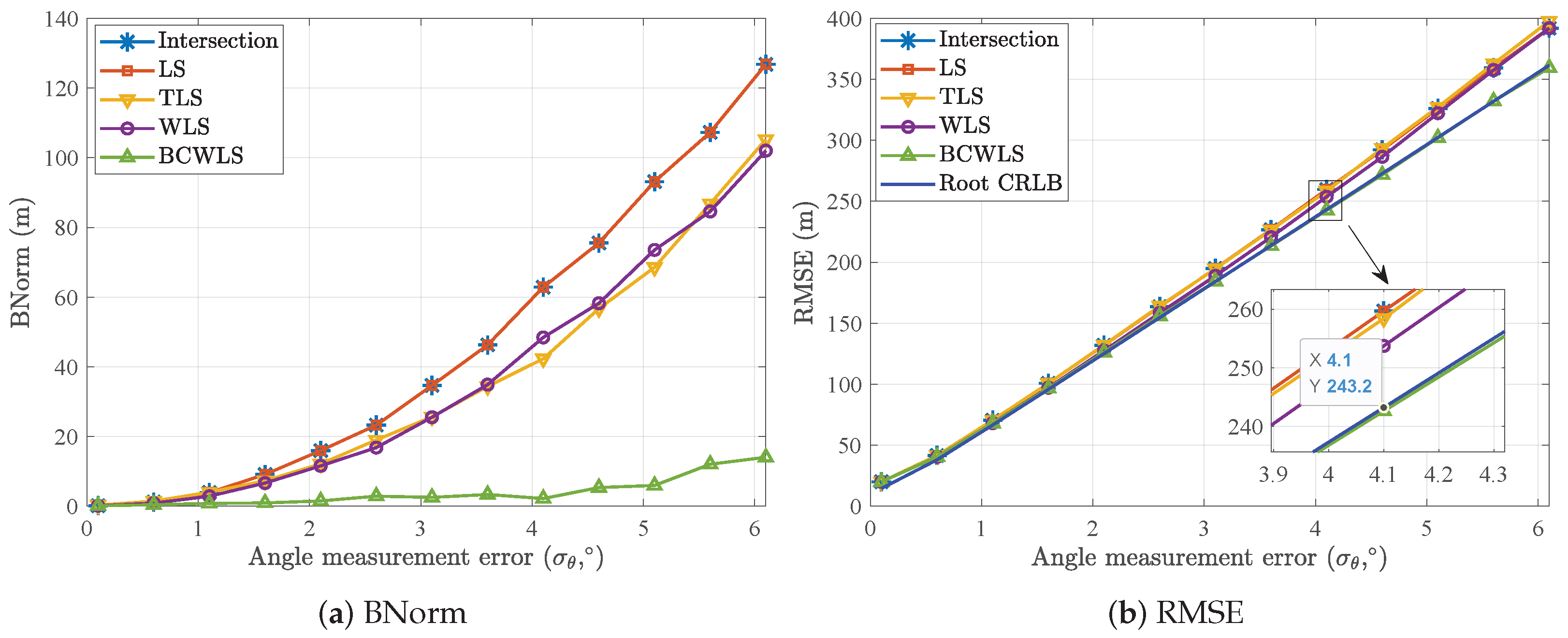
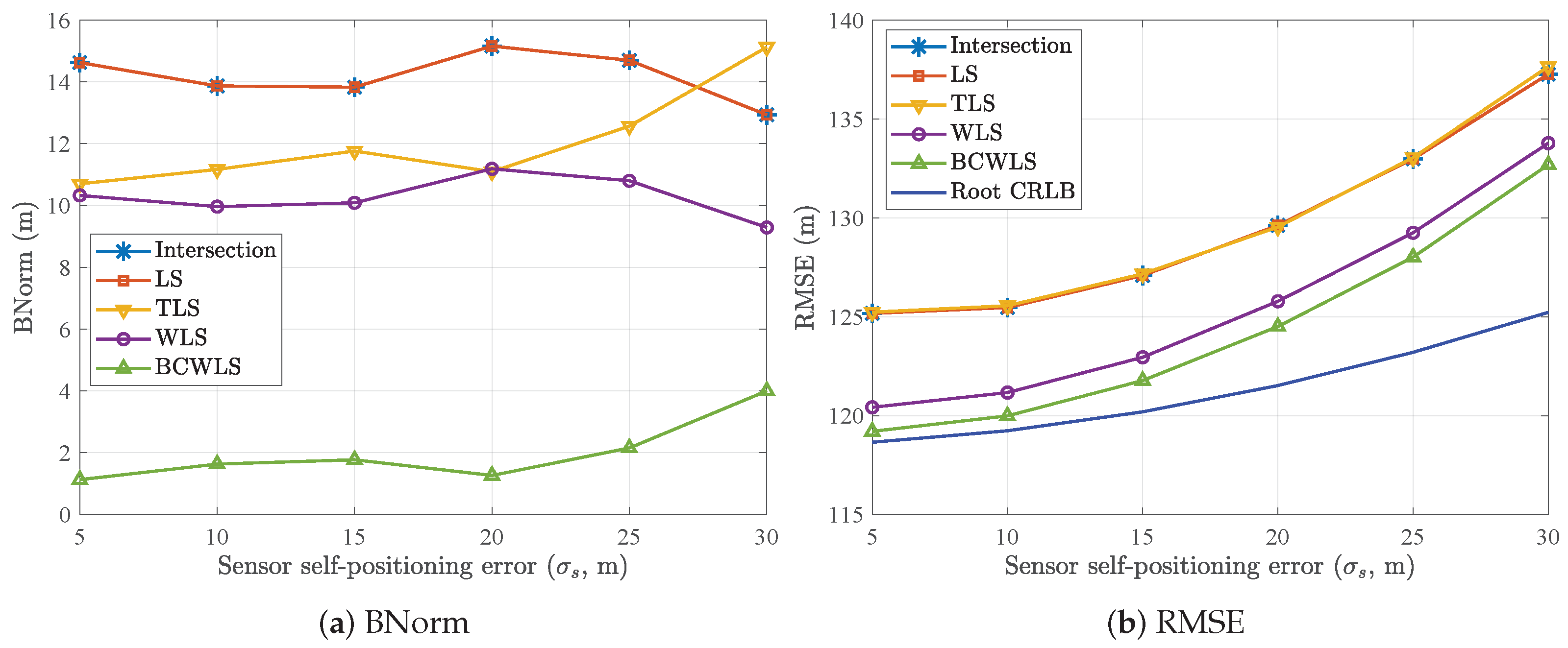
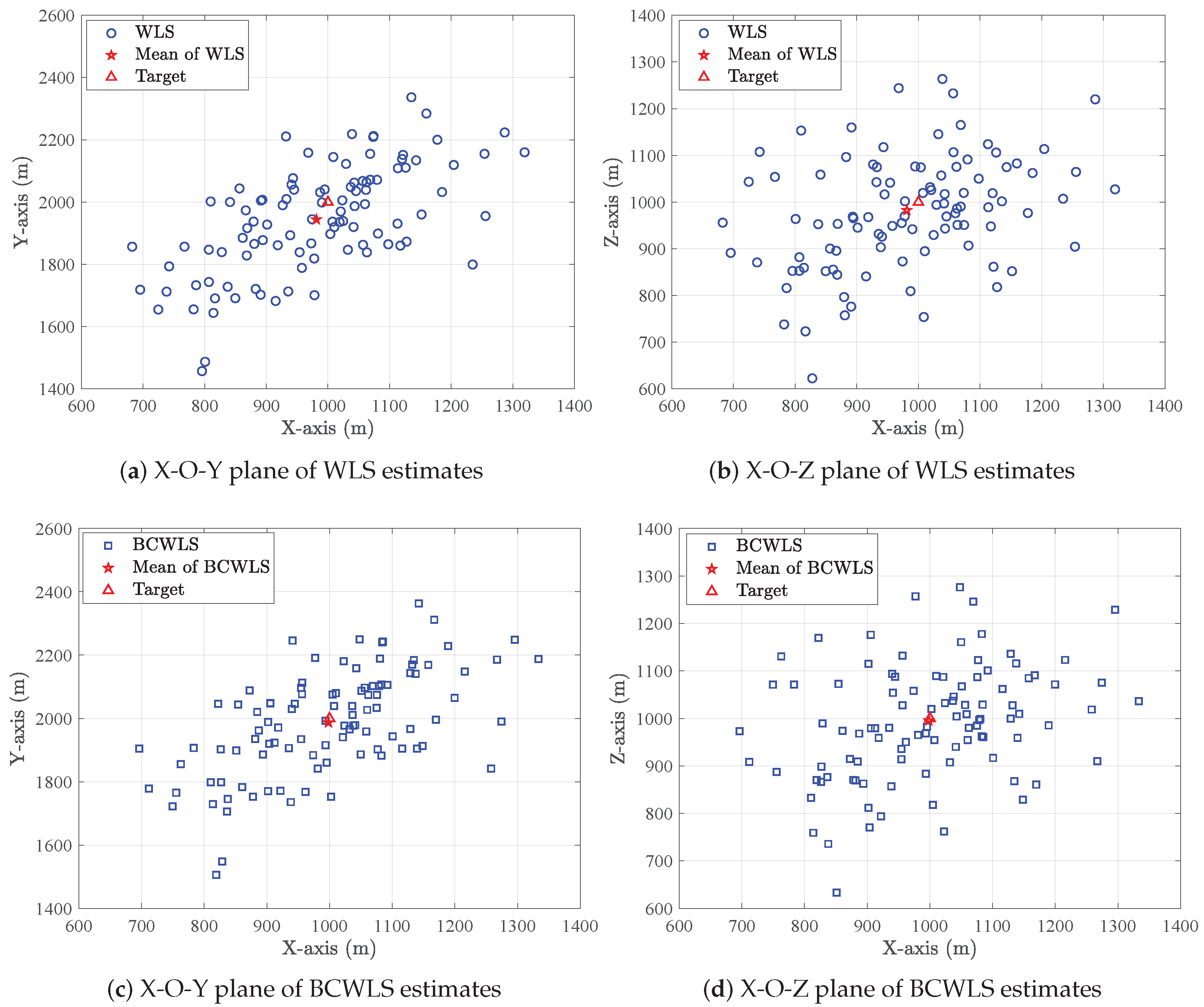
3.2. The Impacts of Sensor Self-Positioning Noise and Angle Measurement Noise

To evaluate the influence of the measurement noise level on the target localization accuracy, we compared the RMSE and BNorm performance of the above algorithms under different error conditions. First, we evaluated the impact of the angle measurement noise level on the target localization accuracy of each algorithm. We fixed the sensor self-positioning noise level ${\sigma }_s$ at 10 m, and the angle measurement noise level varied from 0.1° to 6.1° at intervals of 0.5°. Figure 2 illustrates the impact of angle measurement noise level on the target localization performance of the above target position estimators.

Form Figure 2, it appears that the proposed intersection localization algorithm and the LS algorithm had the same BNorm and RMSE, verifying the inference that the target position solutions of the two algorithms were equal. The BNorm of the TLS and WLS algorithms was very close, slightly better than that of LS algorithm. In addition, the BCWLS algorithm had the smallest BNorm among several algorithms, which showed the effectiveness of the proposed algorithm. We can see that the BNorm of all the methods was less than 5 m if the angle measurement noise level was less than 1.1°. However, with the increase in ${\sigma }_{\theta }$, the BNorm of the other methods, other than the BCWLS algorithm, increased rapidly. When the ${\sigma }_{\theta }$ was 4.1°, the BNorm of the WLS and TLS algorithms was close to 40 m, the BNorm of the LS algorithm and intersection localization algorithm was close to 60 m, while the BNorm of BCWLS algorithm was still less than 5 m. Form Figure 2b, it can be seen that the proposed BCWLS algorithm had the best RMSE among the above algorithms, and its RMSE was much closer to the root CRLB.

Next, we evaluated the impact of sensor self-positioning accuracy on target localization performance. We fixed the angle measurement noise level ${\sigma }_{\theta }$ at 2°, and the sensor self-positioning noise level ${\sigma }_s$ varied from 5 m to 30 m, at intervals of 5 m. Figure 3 illustrates the impact of the sensor self-positioning noise level on the target localization performance of the above target position estimators. Figure 3a gives the BNorm results of the estimators. It shows that the BCWLS algorithm had the best BNorm performance among the considered algorithms. The BNorm results of the TLS and WLS methods were very close to each other and slightly better than the BNorm of the LS method and intersection localization method. In addition, we can see that the BNorm of the above various algorithms remained stable as the sensor self-positioning noise level ${\sigma }_s$ increased. The reason is that the bias of the target position estimators is caused by the nonlinearity of the angle-only measurement and the target position. The impacts of the sensor self-positioning noise level on the RMSE of several estimators are shown in Figure 3b. It is obvious that the BCWLS method had the best RMSE results among several algorithms. The RMSE of the TLS algorithm, LS algorithm, and intersection localization method was very close and larger than that of the WLS method. In addition, the LS algorithm and intersection localization algorithm had the same RMSE and BNorm results, which further verified the inference that both algorithms had the same target position estimates.

To illustrate the advantages of the BCWLS algorithm in terms of bias, we directly show the target position estimates of the WLS and BCWLS algorithms. Figure 4 shows the 100 target position estimates of the two methods under the conditions ${\sigma }_{\theta }=4°$ and ${\sigma }_s=10$ m. The shapes ◯ and □ represent the target position estimates obtained by the WLS and BCWLS methods, respectively. The shape Δ represents the true position of the target. The shape ✩ is the mean of the 100 target position estimates obtained by the WLS or BCWLS method. It should be noted that the measurements used for the 100 target position estimates by these two methods were the same. We can see that the mean of the target position estimates by the WLS method deviates from the true position of target. In contrast, the mean of the target position estimates by BCWLS method is closer to the true value of the target position. Thus, the BCWLS method generally has a better localization performance than the WLS method.

3.3. The Impact of the Number of Sensors

It is well known that target localization performance depends to a large extent on the number of sensors and the geometry of the sensors and the target. Therefore, we changed the number of sensors to three, removed the fourth sensor in Table 1, and kept the positions of the remaining sensors and the target unchanged.

Figure 5 illustrates the target localization performance of the considered algorithms with ${\sigma }_s$ fixed at 10 m and ${\sigma }_{\theta }$ varying from 0.1° to 6.1° in the case of three sensors. Form Figure 2a and Figure 5a, it is obvious that after the removal of sensor $\#4$, the BNorm of several algorithms changed under different angle measurement noise levels. Under the condition of ${\sigma }_{\theta }=4.1°$, when the number of sensors was four, the BNorm of the LS algorithm and intersection localization algorithm was about 45 m, and the BNorm of the BCWLS algorithm was about 5 m. However, after removing sensor $\#4$, the BNorm of the intersection localization algorithm, LS, TLS, and WLS methods was very close, only about 30 m, and the BNorm of BCWLS was also about 5 m. Therefore, according to the results, increasing the number of sensors may not necessarily improve the BNorm performance of target position estimators, and the geometry between the sensors and the target needs to be considered. Form Figure 2b and Figure 5b, it is obvious that after removing sensor $\#4$, the RMSE of BCWLS algorithm was also the smallest among the considered algorithms. In addition, after removing sensor $\#4$, under the different conditions of angle measurement noise level, the root CRLB of the target position estimates remained almost unchanged compared to that without removal. For example, in the case of ${\sigma }_{\theta }=4.1°$, before removing sensor $\#4$, the root CRLB of target position estimates was $243.2$ m, and after removing sensor $\#4$, the root CRLB was $252.1$ m, with only a difference of about $8.9$ m.

Figure 6 shows the target localization performance of the considered algorithms at a fixed ${\sigma }_{\theta }$ of 2° and ${\sigma }_s$ varying from 5 m to 30 m in the case of three sensors. Form Figure 6a and Figure 3a, we can see that the BNorm of the BCWLS algorithm was the smallest among the tested algorithms. In addition, by comparing Figure 6a and Figure 3a, we can see that after removing sensor $\#4$, the BNorm of the intersection localization method and LS method decreased approximately from 14 m to 7 m, and the BNorm of the TLS and WLS methods decreased approximately from 10 m to 7 m. Therefore, the results further demonstrate that increasing the number of sensors may not necessarily improve the BNorm performance of target position estimates, and it is necessary to consider the geometry of the sensors and the target. Form Figure 6b and Figure 3b, we can see that the RMSE of these methods was very close before and after removing sensor $\#4$. The RMSE of the BCWLS method was also the smallest among the considered algorithms in different cases of sensor self-positioning noise levels. The results verify the superiority of the positioning accuracy of the BCWLS method among the above methods.

3.4. The Computational Cost

According to the analysis in Section 2.3, as the size of the coefficient matrices $\mathbf{E}$ and $\mathbf{A}$ of the intersection localization method and LS method is $3\times L_m$ and $2L_m\times 3$, respectively, the intersection localization method theoretically involves fewer multiplication and addition operations and has a lower computational cost. In order to study the computational cost of the above algorithms, we recorded the required computational time of these algorithms under the same conditions.

Table 2. The total computation time of the intersection localization method, LS, TLS, WLS, and BCWLS algorithms across 20,000 Monte Carlo runs, absolute and relative.

Method	Intersection	LS	TLS	WLS	BCWLS
Absolute time (ms)	312.05	490.21	675.60	1130.04	1515.82
Relative time	0.64	1	1.38	2.31	3.09

shows the total time of various algorithms across 20,000 Monte Carlo runs, where the positions of the sensors and the target were set as in Table 1. It illustrates that the time of the intersection localization method was the shortest. Compared with the LS algorithm, the intersection localization algorithm reduced the total time by about $178.16$ ms in 20,000 simulations, with a reduction ratio of approximately $36\%$. Therefore, the target position estimates of the intersection localization algorithm and the LS algorithm were the same, but the computational cost of the intersection localization algorithm was smaller. Since the target position estimates were obtained by an SVD of the augmented matrix $\mathbf{C}$, the computational cost of the TLS algorithm was higher than that of the LS algorithm. In addition, the time of the BCWLS algorithm increased approximately $385.78$ ms compared to that of the WLS algorithm, because the BCWLS algorithm has a bias-compensation operation compared to the WLS algorithm, resulting in a higher computational cost.

4. Discussion

In this paper, we first presented an intersection localization method to estimate the target position based on angle-only measurements. A theoretical analysis showed that this method had the same target position solution as the LS method, but due to the smaller size of the coefficient matrix, the computational cost was lower. The simulation results verified that the intersection localization method and the LS method had the same target position solution and a lower computational cost under the same conditions. Since the size of the coefficient matrices for both the intersection localization and the LS methods is proportional to the number of angle-only measurements, the more angle-only measurements there are, the more computational cost of the intersection localization decreases compared to the LS method.

In addition, through a theoretical analysis, we found that the WLS target localization method with angle-only measurements was biased due to the correlation between the coefficient matrix and the noise vector. Therefore, we further presented a BCWLS method by estimating the bias of the WLS method. This method could reduce the localization bias to a certain extent. The simulation results showed that in different scenarios, the BCWLS method had a smaller BNorm and RMSE compared to the intersection localization method, LS method, TLS method, and WLS method. In addition, the results showed that the BCWLS method could approximately achieve the CRLB. However, due to the addition of a bias-compensation step in the BCWLS method, the computational cost was higher than that of the WLS method.

In order to investigate the impact of the number of sensors on the target positioning accuracy, we removed one sensor from the original sensor network in a simulation and compared the positioning accuracy of various algorithms before and after removal. The results showed that the RMSE and BNorm of various algorithms under different error conditions before and after removal were very close, and the BNorm of various algorithms after removal was even smaller. Therefore, when increasing the number of the sensors to improve the target positioning accuracy, it should be noted that the geometry of the sensors and the target plays an important role. If the placement of new sensors is improper, it is likely to have the opposite effect.

5. Conclusions

This paper studied the source localization problem with angle-only measurements in a passive sensor network. We first presented an intersection localization method that was obtained by minimizing the distances between lines formed by angle-only measurements. Starting from the angle measurement formula, we studied the LS algorithm by solving the target position equations constructed from angle measurements. Comparing the closed-form solutions of the intersection localization algorithm and the LS algorithm, we proved that the two algorithms had the same target position solution. However, since the coefficient matrix of the intersection localization method was smaller, its computational cost was lower than that of the LS method. Furthermore, we studied the TLS method, which takes into account not only the errors in the data vector but also the errors in the coefficient matrix. In contrast, the LS method only considers the error in the data vector. The intersection localization method, LS, and TLS methods do not take into account the difference in measurements errors of different sensors. In practice, the measurement noise level of each sensor may be different. We studied the WLS method by considering the difference in measurement accuracy of sensors. Since the coefficient matrix and the pseudolinear noise vector of the WLS method are correlated, the WLS method is biased, especially at high measurement noise level. To reduce the bias, we presented a BCWLS method by estimating the correlation between the coefficient matrix and pseudolinear noise vector. The BCWLS method had a higher accuracy of the target position estimate than the WLS method. On the other hand, due to the addition of bias-compensation steps, the computational cost of the BCWLS method also increased. Finally, we derived the CRLB of the target localization based on angle-only measurements to evaluate the positioning performance of the above algorithms.

The numerical simulations showed that the intersection localization algorithm and LS algorithm had the same localization results, verifying the theoretical derivation. We also analyzed the impacts of the measurement noise level on the target localization performance of the above target position estimators, including angle measurement noise and sensor self-positioning noise. The target localization performance advantages of the BCWLS method were verified by a numerical simulation. Furthermore, the running time of the considered methods was compared, and the results showed that the intersection localization method had the lowest computational cost.

In this paper, we assumed that the self-positioning noise and the angle measurement noise both followed a zero-mean Gaussian distribution. However, in practice, this assumption may not be valid. In particular, if the passive sensor is mounted on a motion platform, the sensor self-positioning noise may not be zero-mean. Therefore, in the future, we will study the target localization based on angle-only measurements with a non-Gaussian noise background.

References

1. Olson, E.; Leonard, J.J.; Teller, S. Robust Range-Only Beacon Localization. IEEE J. Ocean. Eng. 2006, 31, 949–958. [Google Scholar] [CrossRef]
2. Hamdollahzadeh, M.; Amiri, R.; Behnia, F. Moving Target Localization in Bistatic Forward Scatter Radars: Performance Study and Efficient Estimators. IEEE Trans. Aerosp. Electron. Syst. 2020, 56, 1582–1594. [Google Scholar] [CrossRef]
3. Sadeghi, M.; Behnia, F.; Amiri, R.; Farina, A. Target Localization Geometry Gain in Distributed MIMO Radar. IEEE Trans. Signal Process. 2021, 69, 1642–1652. [Google Scholar] [CrossRef]
4. Famoriji, O.J.; Shongwe, T. Source Localization of EM Waves in the Near-Field of Spherical Antenna Array in the Presence of Unknown Mutual Coupling. Wirel. Commun. Mob. Comput. 2021, 2021, 3237219. [Google Scholar] [CrossRef]
5. Wang, C.L.; Yang, R.J. Research on Airborne Infrared Passive Location Method Based on Orthogonal Multi-station Triangulation. Laser Infrared 2007, 11, 1184–1187+1191. [Google Scholar]
6. Kazemi, S.A.R.; Amiri, R.; Behnia, F. Efficient Closed-Form Solution for 3-D Hybrid Localization in Multistatic Radars. IEEE Trans. Aerosp. Electron. Syst. 2021, 57, 3886–3895. [Google Scholar] [CrossRef]
7. Yang, J.; Liu, C.; Huang, J.; Hu, D.; Zhao, C. Overcoming Unknown Measurement Noise Powers in Multistatic Target Localization: A Cyclic Minimization and Joint Estimation Algorithm. Radioengineering 2023, 32, 415–424. [Google Scholar] [CrossRef]
8. Wang, Y.; Ho, K.C. An Asymptotically Efficient Estimator in Closed-Form for 3-D AOA Localization Using a Sensor Network. IEEE Trans. Wirel. Commun. 2015, 14, 6524–6535. [Google Scholar] [CrossRef]
9. Bai, G.; Liu, J.; Song, Y.; Zuo, Y. Two-UAV Intersection Localization System Based on the Airborne Optoelectronic Platform. Sensors 2017, 17, 98. [Google Scholar] [CrossRef]
10. Peng, S.; Zhao, Q.; Ma, Y.; Jiang, J. Research on the technology of cooperative dual-station position based on passive radar system. In Proceedings of the 2020 3rd International Conference on Unmanned Systems (ICUS), Harbin, China, 27–28 November 2020; pp. 611–614. [Google Scholar] [CrossRef]
11. Chen, Y.; Wang, L.; Zhou, S.; Chen, R. Signal Source Positioning Based on Angle-Only Measurements in Passive Sensor Networks. Sensors 2022, 22, 1554. [Google Scholar] [CrossRef]
12. Doğançay, K. 3D Pseudolinear Target Motion Analysis From Angle Measurements. IEEE Trans. Signal Process. 2015, 63, 1570–1580. [Google Scholar] [CrossRef]
13. Nguyen, N.H.; Doğançay, K.; Kuruoglu, E.E. An Iteratively Reweighted Instrumental-Variable Estimator for Robust 3-D AOA Localization in Impulsive Noise. IEEE Trans. Signal Process. 2019, 67, 4795–4808. [Google Scholar] [CrossRef]
14. Jia, T.; Wang, H.; Shen, X.; Jiang, Z.; He, K. Target localization based on structured total least squares with hybrid TDOA-AOA measurements. Signal Process. 2018, 143, 211–221. [Google Scholar] [CrossRef]
15. Wells, D.E.; Krakiwsky, E.J. The Method of Least Squares; Department of Surveying Engineering, University of New Brunswick Canada: Fredericton, NB, Canada, 1971; Volume 18. [Google Scholar]
16. Doğançay, K. On the bias of linear least squares algorithms for passive target localization. Signal Process. 2004, 84, 475–486. [Google Scholar] [CrossRef]
17. Doğançay, K. Bearings-only target localization using total least squares. Signal Process. 2005, 85, 1695–1710. [Google Scholar] [CrossRef]
18. Golub, G.H.; van Loan, C.F. An Analysis of the Total Least Squares Problem. SIAM J. Numer. Anal. 1980, 17, 883–893. [Google Scholar] [CrossRef]
19. Markovsky, I.; Van Huffel, S. Overview of total least-squares methods. Signal Process. 2007, 87, 2283–2302. [Google Scholar] [CrossRef]
20. Dogancay, K. Relationship Between Geometric Translations and TLS Estimation Bias in Bearings-Only Target Localization. IEEE Trans. Signal Process. 2008, 56, 1005–1017. [Google Scholar] [CrossRef]
21. Wu, W.; Jiang, J.; Fan, X.; Zhou, Z. Performance analysis of passive location by two airborne platforms with angle-only measurements in WGS-84. Infrared Laser Eng. 2015, 44, 654–661. [Google Scholar]
22. Frew, E.W. Sensitivity of cooperative target geolocalization to orbit coordination. J. Guid. Control. Dyn. 2008, 31, 1028–1040. [Google Scholar] [CrossRef]
23. Zhang, Y.; Li, Y.; Qi, G.; Sheng, A. Cooperative Target Localization and Tracking with Incomplete Measurements. Int. J. Distrib. Sens. Netw. 2014, 2014. [Google Scholar] [CrossRef]
24. Pang, F.; Doğançay, K.; Nguyen, N.H.; Zhang, Q. AOA Pseudolinear Target Motion Analysis in the Presence of Sensor Location Errors. IEEE Trans. Signal Process. 2020, 68, 3385–3399. [Google Scholar] [CrossRef]
25. Ghaderpour, E.; Antonielli, B.; Bozzano, F.; Scarascia Mugnozza, G.; Mazzanti, P. A fast and robust method for detecting trend turning points in InSAR displacement time series. Comput. Geosci. 2024, 185, 105546. [Google Scholar] [CrossRef]
26. Hu, J.; Li, Z.; Ding, X.; Zhu, J.; Sun, Q. Spatial–temporal surface deformation of Los Angeles over 2003–2007 from weighted least squares DInSAR. Int. J. Appl. Earth Obs. Geoinf. 2013, 21, 484–492. [Google Scholar] [CrossRef]
27. Sun, Y.; Ho, K.C.; Wan, Q. Eigenspace Solution for AOA Localization in Modified Polar Representation. IEEE Trans. Signal Process. 2020, 68, 2256–2271. [Google Scholar] [CrossRef]
28. Shao, H.J.; Zhang, X.P.; Wang, Z. Efficient Closed-Form Algorithms for AOA Based Self-Localization of Sensor Nodes Using Auxiliary Variables. IEEE Trans. Signal Process. 2014, 62, 2580–2594. [Google Scholar] [CrossRef]
29. Doğançay, K. Passive emitter localization using weighted instrumental variables. Signal Process. 2004, 84, 487–497. [Google Scholar] [CrossRef]
30. Zhou, S.; Wang, L.; Liu, R.; Chen, Y.; Peng, X.; Xie, X.; Yang, J.; Gao, S.; Shao, X. Signal Source Localization with Long-Term Observations in Distributed Angle-Only Sensors. Sensors 2022, 22, 9655. [Google Scholar] [CrossRef] [PubMed]
31. Wang, L.; Zhou, S.; Chen, Y.; Xie, X. Bias compensation Kalman filter for 3D angle-only measurements target traking. In Proceedings of the International Conference on Radar Systems (RADAR 2022), Edinburgh, UK, 24–27 October 2022; Volume 2022, pp. 546–551. [Google Scholar] [CrossRef]
32. Rao, S.K. Pseudo-linear estimator for bearings-only passive target tracking. IEEE Proc. Radar Sonar Navig. 2001, 148, 16–22. [Google Scholar] [CrossRef]
33. He, S.; Wang, J.; Lin, D. Three-Dimensional Bias-Compensation Pseudomeasurement Kalman Filter for Bearing-Only Measurement. J. Guid. Control. Dyn. 2018, 41, 2678–2686. [Google Scholar] [CrossRef]
34. Mallick, M.; Morelande, M.; Mihaylova, L.; Arulampalam, S.; Yan, Y. Angle-Only Filtering in Three Dimensions; Wiley: Hoboken, NJ, USA, 2016; pp. 3–42. [Google Scholar]
35. Arasaratnam, I.; Haykin, S. Cubature Kalman Filters. IEEE Trans. Autom. Control. 2009, 54, 1254–1269. [Google Scholar] [CrossRef]
36. Julier, S.; Uhlmann, J. Unscented filtering and nonlinear estimation. Proc. IEEE 2004, 92, 401–422. [Google Scholar] [CrossRef]
37. Mao, W.L. GPS Interference Mitigation Using Derivative-free Kalman Filter-based RNN. Radioengineering 2016, 25, 518–526. [Google Scholar] [CrossRef]
38. Yu, J.Y.; Coates, M.J.; Rabbat, M.G.; Blouin, S. A Distributed Particle Filter for Bearings-Only Tracking on Spherical Surfaces. IEEE Signal Process. Lett. 2016, 23, 326–330. [Google Scholar] [CrossRef]
Figure 1. Three-dimensional target localization scenario.
Remotesensing 16 01319 g001
Figure 2. The BNorm and RMSE of the target position estimators with σ s fixed at 10 m and σ θ varying from 0.1° to 6.1°.
Remotesensing 16 01319 g002
Figure 3. The BNorm and RMSE of the target position estimators with σ θ fixed at 2° and σ s varying from 5 m to 30 m.
Remotesensing 16 01319 g003
Figure 4. The target position estimates of the WLS and BCWLS algorithms on the X-O-Y plane and X-O-Z plane. ◯ represents the WLS estimates of the target position. □ represents the BCWLS estimates of the target position. Δ represents the true position of the target. ✩ represents the mean of target position estimates.
Remotesensing 16 01319 g004
Figure 5. The BNorm and RMSE of the target position estimators with σ s fixed at 10 m and σ θ varying from 0.1° to 6.1° in the case of 3 sensors.
Remotesensing 16 01319 g005
Figure 6. The BNorm and RMSE of the target position estimators with σ θ fixed at 2° and σ s varying from 5 m to 30 m in the case of 3 sensors.
Remotesensing 16 01319 g006