High Spatiotemporal Estimation of Reservoir Evaporation Water Loss by Integrating Remote-Sensing Data and the Generalized Complementary Relationship

Abstract

Accurately estimating the reservoir evaporation loss is crucial for water resources management. The existing research on reservoir evaporation loss estimates primarily focuses on large spatiotemporal scales and neglects the rapid dynamic changes to reservoirs’ surface area. For reservoirs essential for frequent flood control and regular water supply, high spatiotemporal evaporation data are crucial. By integrating remote sensing and the evaporation model, this study proposes a new method for the high spatiotemporal estimation of the evaporation losses from reservoirs. The proposed method is applied to the largest artificial freshwater lake in Asia, i.e., Danjiangkou (DJK) Reservoir. The daily reservoir water surface area is extracted at a spatial resolution of 30 m during the period 2014–2018 based on the Enhanced Spatial and Temporal Adaptive Reflectance Fusion Model (ESTARFM). The daily evaporation rate is estimated at a spatial resolution of 100 m using the generalized complementary relationship (GCR). The results show that the water surface area of the DJK Reservoir exhibits rapid and frequent fluctuations from 2015 to 2018, with a multi-year average area of 731.9 km² and a maximum and minimum difference of 304 km². Significant seasonal variations are observed in both the evaporation rate and volume, with a multi-year average evaporation rate of 806 mm and evaporation volume of 595 million m³. The estimated results align well with three other independent estimates, indicating that the GCR is capable of water surface evaporation estimation. Further analysis suggests that the data resolution has a great influence on the evaporative water loss from the reservoir. The estimated mean annual evaporation volume based on the 1000 m resolution water surface area data is 14% lower than that estimated using the 30 m resolution water surface area data. This study not only provides a new method for the high spatiotemporal estimation of reservoir evaporation by integrating remote-sensing data and the GCR method but also highlights that reservoir evaporation water loss should be quantified using the volume rather than the rate and that the estimated loss is noticeably affected by the estimation spatial resolution.

1. Introduction

Water surface evaporation refers to the process in which water molecules on the surface of a water body transition from a liquid state to a gaseous state. This phenomenon constitutes a vital component of the hydrological cycle and has significant implications for water resources management [1], climate studies [2,3], and the functioning of ecosystems [4]. Reservoir water resources play a pivotal role in the sustainable societal and economic development of all nations. Due to the expansive open water areas of reservoirs, significant amounts of water are lost through evaporation annually [5]. Therefore, accurately quantifying the reservoir evaporative water loss is crucial for water resources management and sustainable utilization, and it can provide fundamental data and a basis for water resource protection [6,7].

The dynamics of reservoir evaporative water loss are influenced by both the water surface area and the evaporation rate. Most of the current research predominantly focuses on variations in the evaporation rate rather than the overall evaporation loss [8,9,10]. Evaporation rates alone may not provide an accurate depiction of the reservoir evaporation loss, especially for reservoirs where water surface area changes are usually huge due to floodwater utilization. Current studies on the quantification of evaporation losses from reservoirs mostly concentrate on large (e.g., globe and nation) or point (e.g., experimental site) scales [11,12,13,14]. The large-scale studies provide a fundamental understanding of terrestrial water surface evaporation at the global and national scales. However, the spatiotemporal resolutions of these estimations are relatively low and thus rapid changes in the water surface area and the consequences for reservoir evaporation are overlooked. The water surface of a reservoir can change rapidly over a few days, and it can significantly influence evaporation estimation [15]. Experimental site-scale research provides more accurate data, while the acquisition of data is challenging, and such data can only provide limited information on whole reservoir-scale evaporation [16]. Therefore, to acquire more detailed and continuous evaporation information from the reservoir, high spatiotemporal reservoir surface area and evaporation rate data are needed [17,18].

The reservoir surface area is usually inferred from in situ water level measurements. However, this method has some limitations in obtaining the continuous, accurate, and spatially distributed reservoir water surface area [19], which is critically important under the influence of artificial control for floodwater utilization [20]. Reservoir water level variations during the flood season can be up to tens of meters and spatiotemporal changes are highly dynamic, necessitating high temporal and spatial resolution for effectively monitoring changes in the water surface area [21]. Remote sensing has advantages in accurately obtaining the water surface area and has become the mainstream method in hydrology research [22,23,24]. Landsat-8 and MODIS are proven to have relative spatial and temporal advantages for water body monitoring [25]. However, there is a trade-off between high temporal and spatial resolutions, so it is necessary to adopt an image fusion algorithm to integrate the advantages of the two observations to obtain long-term, continuous and accurate time series of the water surface area [26]. Gao, et al. [27] introduced the Spatial and Temporal Adaptive Reflectance Fusion Model (STARFM), and the fusion results of this model are particularly suitable for monitoring rapidly changing land features at the regional scale. Subsequently, scholars have advanced this method, such as Zhu et al. [28], who proposed the Enhanced Spatial and Temporal Adaptive Reflectance Fusion Model (ESTARFM). This model has improved the capacity of the STARFM in the heterogeneous and changing region [29], and it has been applied widely [30]. Remote sensing has significantly improved our capacity to accurately map highly dynamic variations in the reservoir surface area, especially during the flood season.

Various methods have been successfully applied to estimate water surface evaporation rates, such as the Pan evaporation method [31], eddy covariance method (EC) [32], Bowen ratio energy budget method (BREB) [33], mass balance approach [34] and Penman equation [35,36]. The Pan evaporation method, EC and BREB rely on point observations, requiring station deployment for estimating evaporation. However, due to cost and site constraints, the limited station density makes them unsuitable for large-scale evaporation estimation. The mass balance approach is data intensive, requiring inputs of inflow, outflow, storage change, and water use data [37]. However, the intensive data requirement can lead to considerable errors [38]. The Penman equation is the most common method among the various combination equation methods [39]. It assumes that the relationship between the potential evaporation (${\mathrm{E}}_{\mathrm{p}\mathrm{a}}$) and actual evaporation (${\mathrm{E}}_{\mathrm{a}}$) is proportional. But, the Penman method neglects the feedback of evaporation on the near-surface atmosphere [40]. The generalized complementary relationship (GCR) [41] is the latest form of complementary principle [42]. It considers the complex feedback of evaporative rate changes on atmospheric conditions and attributes the complex evaporation surface and atmosphere interactions to the changes in several meteorological elements, including the temperature, humidity, etc. [43]. The input data for the GCR method are mostly routine meteorological observations [44]. Recently, it has been validated and successfully applied in various climates and landscapes globally [41,45,46]. However, it has rarely been applied to estimate water surface evaporation and thus needs further verification.

This study proposes a new method by integrating the ESTARFM and GCR to allow for the high spatiotemporal estimation of evaporation from reservoirs. Danjiangkou (DJK) Reservoir, the largest artificial freshwater lake in Asia, is chosen as the study area. The DJK Reservoir serves as the source for the South-to-North Water Diversion Middle Route Project (SNWDP) that benefits more than 100 million people; thus, understanding its evaporation is important for water resources management. Specifically, our main objectives are: (1) to derive the water surface area of the DJK Reservoir at high spatial and temporal resolution; (2) to estimate the evaporation rate and volume of the DJK Reservoir at high spatial and temporal resolution; and (3) to demonstrate the capability of the GCR for estimating large reservoir water surface evaporation.

2. Methods

2.1. Surface Area Extraction

The ESTARFM is utilized for the fusion of high-resolution (Landsat) and coarse (MODIS) images [30]. The model takes into account the spatial variability of pixel reflectance, the spectral similarity between central and neighboring pixels, and temporal changes in reflectance values, effectively enhancing the fusion accuracy. Currently, this model has been widely applied in various complex and fragmented landscapes.

The ESTARFM requires two pairs of Landsat and MODIS images at the base date ($t_0$: $t_1$ and $t_2$) and MODIS images for the predicted time to generate Landsat images for the predicted time. Errors in the geometric and atmospheric corrections of the images are overlooked during the fusion process. However, systematic differences in surface reflectance may exist among images from different sensors. Hence, the relationship between the Landsat and MODIS reflectance with homogeneous land cover can be described by a linear model, which is expressed as:

$$L\left(x,y,t_k,b\right)=M\left(x,y,t_k,b\right)+{\epsilon }_k$$

(1)

where ($x,y$) is a given pixel location for both the Landsat (L) and MODIS (M) images, $b$ represent the predicted band, $t_k$ is the acquisition date, and ${\epsilon }_k$ represents the difference between the observed MODIS and Landsat surface reflectance.

The algorithm further assumes that the system error (i.e., ${\epsilon }_k$ in Equation (1)) is the same between periods [27]; thus, Equation (1) can be rewritten to approximate the Landsat reflectance at the predicted date ($t_p$) as:

$$L\left(x,y,t_p,b\right)=L\left(x,y,t_0,b\right)+(M\left(x,y,t_p,b\right)-M\left(x,y,t_0,b\right))$$

(2)

Simultaneously, the ESTARFM algorithm introduces neighboring homogeneous pixels with similar spectral characteristics as auxiliary information to improve the fusion accuracy. Therefore, within a moving window, the predicted reflectance of the center pixel is as follows:

$$L\left(\frac{x_w}{2},\frac{y_w}{2},t_p,b\right)=L\left(\frac{x_w}{2},\frac{y_w}{2},t_0,b\right)+{\sum }_{i=1}^N{W}_i\times v_i\times (M\left(x_i,y_i,t_p,b\right)-M\left(x_i,y_i,t_0,b\right))$$

(3)

where $\frac{x_w}{2}$ and $\frac{y_w}{2}$ represent the locations of the central pixel, $\left(x_i,y_i\right)$ is the location of the i-th pixel, $W_i$ is the weight of the i-th similar pixel, $v_i$ is the conversion coefficient of the i-th similar pixel, and $N$ is the number of similar pixels.

To derive the water surface area utilizing the fused images generated by the ESTARFM, the first step involves delineating the land and water for each pixel. Next, the total water surface area is calculated by multiplying the number of classified water pixels by the grid cell size (900 m²). The water surface area of the reservoir for each period is extracted from the 15-day fused time series by Matthew’s water classification algorithm [47]. This approach involves calculating the mean $\left(M\right)$ and standard deviation $\left(S\right)$ of the Modified Normalized Difference Water Index (MNDWI) for regions that are likely to be water and land. Equation (5) is then applied to compute the appropriate threshold value ${\sigma }_{0WD}$:

$${\sigma }_{0WD}\left(t\right)=M_{Water}\left(t\right)+x{S}_{Water}\left(t\right)=M_{Land}\left(t\right)+x{S}_{Land}\left(t\right)$$

(4)

where $M_{Water}$ and $M_{Land}$ represent the means of the water and land pixels, respectively; $S_{Water}$ and $S_{Land}$ represent the standard deviations of the water and land pixels, respectively; and $x$ is a multiplicative factor determined by equating the center and right-hand side terms of the Equation.

The threshold ${\sigma }_{0WD}$ obtained through Equation (5) is applied to classify the reservoir pixels, following the criteria outlined as follows:

$$class\left(x,y,t\right)=\left\{\begin{array}{c}water, if \sigma \left(x,y,t\right)>{\sigma }_0\left(t\right)\\ land, if \sigma \left(x,y,t\right)\le {\sigma }_0\left(t\right)\end{array}\right.$$

(5)

2.2. Evaporation Volume and Rate Estimation

For a comprehensive evaluation of the water loss from the DJK Reservoir, the evaporation volume ($V_E$) is employed as the primary basis for evaluating the reservoir evaporation loss using Equation (1).

$$V_E=E\times \frac{A_S}{1000}$$

(6)

where $V_E$ represents the daily evaporation volume (m³ d⁻¹);$E$represents the daily evaporation rate (mm d⁻¹); and $A_s$ represents the daily water surface area of the reservoir (km²). The daily scale E is calculated using the GCR. $A_s$ is determined through linear interpolation of the water surface areas extracted at 15-day intervals using the ESTARFM. The specific calculation procedure will be elaborated in the following subsection.

The complementary principle reveals the relationship among three types of evaporation [48,49,50]. The first is the actual evaporation ($E$) of a natural land under drying conditions; the second is the evaporation occurring under ample water availability conditions, known as potential evaporation ($E_{po}$); and the third is the evaporation taking place on a small wet surface area, placed in the same environment and surrounded by the drying surface from which $E$ is taking place, referred to as apparent potential evaporation ($E_{pa}$). Under well-watered conditions, all the net radiation is converted into latent heat through evaporation, resulting in $E$, $E_{pa}$, and $E_{po}$ being equal, i.e., $E=E_{po}=E_{pa}$. However, in water-limited situations, $E$ decreases, with a fraction of the net radiation not dissipated through evaporation transforming into sensible heat, increasing $E_{pa}$. The relationship among these three factors follows $E<E_{po}<E_{pa}$. This study adopts the generalized complementary relationship recently proposed by Brutsaert [51], with the model’s formula as follows:

$$E={(\frac{E_{po}}{E_{pa}})}^2(2E_{pa}-E_{po})$$

(7)

where $E_{po}={\alpha }_c{E}_e$, ${\alpha }_c$ is an adjustable parameter of the complementary relationship [45] and $E_e$ represents equilibrium evaporation. The calculation method for $E_e$ is as follows:

$$E_e=\frac{\Delta }{\Delta +\gamma }{Q}_{ne}$$

(8)

where $\Delta$ is the slope of the saturation vapor pressure curve; $\gamma$ is the psychrometric constant; and $Q_{ne}$ represents available energy, measured in $\mathrm{m}\mathrm{m} {\mathrm{d}\mathrm{a}\mathrm{y}}^{-1}$, and the equation is as follows:

$$Q_{ne}=\frac{(R_n-G)}{\lambda }$$

(9)

where $R_n$ is net radiation, measured in W m⁻²; $\lambda$ is the latent heat of vaporization (MJ kg⁻¹); and G is the water heat flux, measured in W m⁻². Due to the relatively small magnitude of G compared to $R_n$ and its difficulty in terms of measurement, especially at smaller timescales, G was neglected in the estimation [9]. $R_n$ is calculated using $R_n=R_{si}-R_{so}+R_{li}-R_{lo}$. $R_{so}$ and $R_{lo}$ are the outgoing shortwave and longwave radiation. $R_{so}$ is obtained using $R_{so}=\alpha R_{si}$, with $\alpha$ the surface albedo determined to be 0.06 [52]. $R_{lo}$ is calculated by equation $R_{lo}={\epsilon }_s\sigma T_a^4,$ with ${\epsilon }_s$the surface emissivity, $\sigma$the Stefan–Boltzmann constant (5.67 × 10⁻⁸, W m⁻² K⁻⁴). The latent heat values to convert the net radiation into evaporation units are calculated using $\lambda =2.501-0.002361T_a$(MJ kg⁻¹), where $T_a$ is the air temperature 2 m above the surface.

The parameter ${\alpha }_c$ is determined using an empirical statistical model established by Brutsaert, Cheng and Zhang [41]:

$${\alpha }_c=\frac{a}{[1+{\left(bK\right)}^c]}$$

(10)

where $a=$ 1.496; $b=$ 0.2948; $c=$0.6697; and K is the aridity index and is estimated as 1.27.

For $E_{pa}$, it can be measured using an evaporative pan [53,54]. Previous studies demonstrated that $E_{pa}$ can be estimated by Penman equations [55].

$$E_{pa}=\frac{\Delta }{\Delta +\gamma }{Q}_{ne}+\frac{\gamma }{\Delta +\gamma }{f}_e\left(u_2\right)(e_1^{\ast }-e_1)$$

(11)

where $u_2$(m s⁻¹) is the average wind speed measured at a height of $z_2$ above the surface, while $e_1$(hPa) is the vapor pressure recorded at a height of $z_1$ above the surface, with the asterisk indicating saturation. For routine meteorological observations, $z_1$ and $z_2$ are 2 m above the surface. The wind function $f_e\left(u_2\right)$ is formulated through the Penman wind function [35] as:

$$f_e\left(u_2\right)=0.26(1+0.54u_2)$$

(12)

The vapor pressure $e_1$ is estimated as $e_1=0.0016077q_{air}Pres$, where $q_{air}$ and $Pres$ are the specific humidity and surface pressure, respectively.

3. Study Area and Data

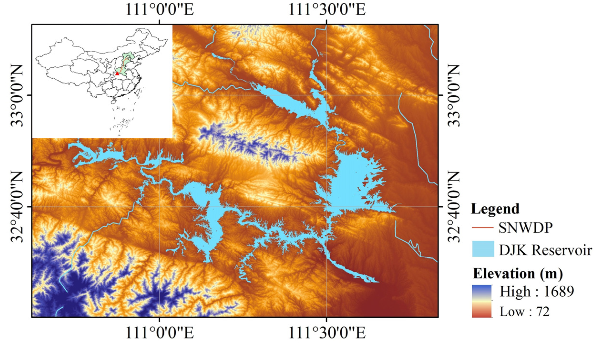
3.1. Study Area

The DJK Reservoir is situated in the middle and upper reaches of the Han River [56], spanning the provinces of Hubei and Henan (32°71′, 111°55′; Figure 1). It is the largest artificial freshwater lake in Asia, serving a crucial role as a water source for the Middle Route of the SNWDP. The reservoir fulfills multiple functions, including flood control, water supply, power generation, irrigation, navigation, and aquaculture [57]. Located in a subtropical monsoon climate [58], the reservoir experiences an average annual temperature of 15.8 °C and an average annual precipitation of 804.3 mm, with higher precipitation levels typically observed in July and September. The reservoir has a water surface area of 546 km² and receives an average annual inflow of 39.48 billion m³, primarily from the Han River and its tributary, the Dan River. The reservoir underwent a dam heightening project starting in 2005, officially completing operations in 2013 [59]. This project raised the normal water level from 157 m to 170 m [60], increasing the reservoir’s maximum storage capacity to 29.05 billion m³. The Middle Route of the SNWDP became operational in December 2014, further impacting the reservoir’s dynamics. The reservoir undergoes multiple cycles of water storage and discharge each year due to various operational requirements, such as flood control, water resource utilization, and power generation, contributing to the highly dynamic nature of the reservoir’s water level. Due to the flat terrain around the reservoir, changes in the water level can result in significant variations in the water surface area.

3.2. Data

Six meteorological variables of the China Meteorological Forcing Dataset (CMFD) [61] were collected as input parameters for the application of the GCR in estimating the evaporation rate. The variables included the 2 m air temperature ($T_a$), surface pressure ($Pres$), specific humidity ($q_{air}$), 10 m wind speed ($WS$), downward shortwave radiation ($R_{si}$), and downward longwave radiation ($R_{li}$). The dataset is available for the period 2014–2018, with a spatial resolution of 0.1° at the daily time scale. The $WS$ data were reduced to 2 m above the surface by a mean reduction factor of 0.795 [(=2/10)^1/7], which is required in the GCR. To explore the influences of different spatial resolution data on evaporation estimation, the input data were linearly downscaled to resolutions of 100 m, 1000 m, and 5000 m to obtain the evaporation rates at different resolutions.

To achieve image fusion, Landsat 8 OLI (Operational Land Imagery) Surface Reflectance and MODIS NBAR (Nadir BRDF-Adjusted Reflectance) imagery were chosen to be input pairs. The fused 15-day water surface series of the DJK Reservoir with a 30 m resolution was generated based on the ESTARFM. To achieve higher temporal resolution, the linear interpolation method was employed to reconstruct the desired daily water surface series.

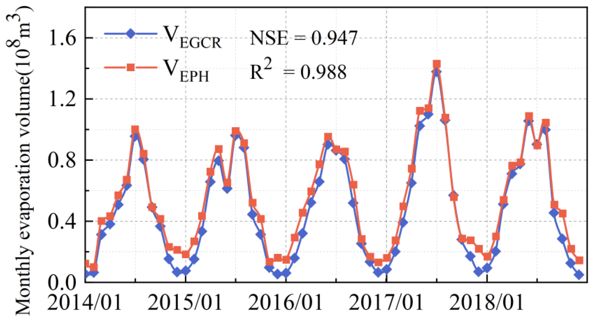
3.3. Independent Datasets and Cross-Validation

To verify the applicability of the GCR in reservoir evaporation estimation, three independent evaporation datasets were further collected, including the Global Land Evaporation Amsterdam Model (GLEAM) [62], ECMWF Reanalysis dataset version 5 (ERA5) [63], and Penman–Monteith–Leuning Evaporation dataset (PML) [64], with the spatial resolution of 0.25°, 0.5°, and 0.05°, respectively. The temporal resolution of the GLEAM and ERA5 is daily, while that of the PML is 8 days. The datasets obtained from the CMFD, GLEAM, ERA5 and PML were resampled to the same resolution (i.e., 100 m) using a local averaging method.

To verify the reliability of the estimated evaporation volumes, a method (PH) proposed by Zhao and Gao [17] was selected as a comparative method, which has been validated using in situ observations. This method incorporates the fetch length into the Penman equation, which requires daily wind direction data from the DJK Reservoir for the years 2014 to 2018. Due to data availability challenges, 3 h interval wind direction data from the Laohekou station (~25 km away) of the National Climate Data Center were used as a substitute and were converted into daily data.

4. Results

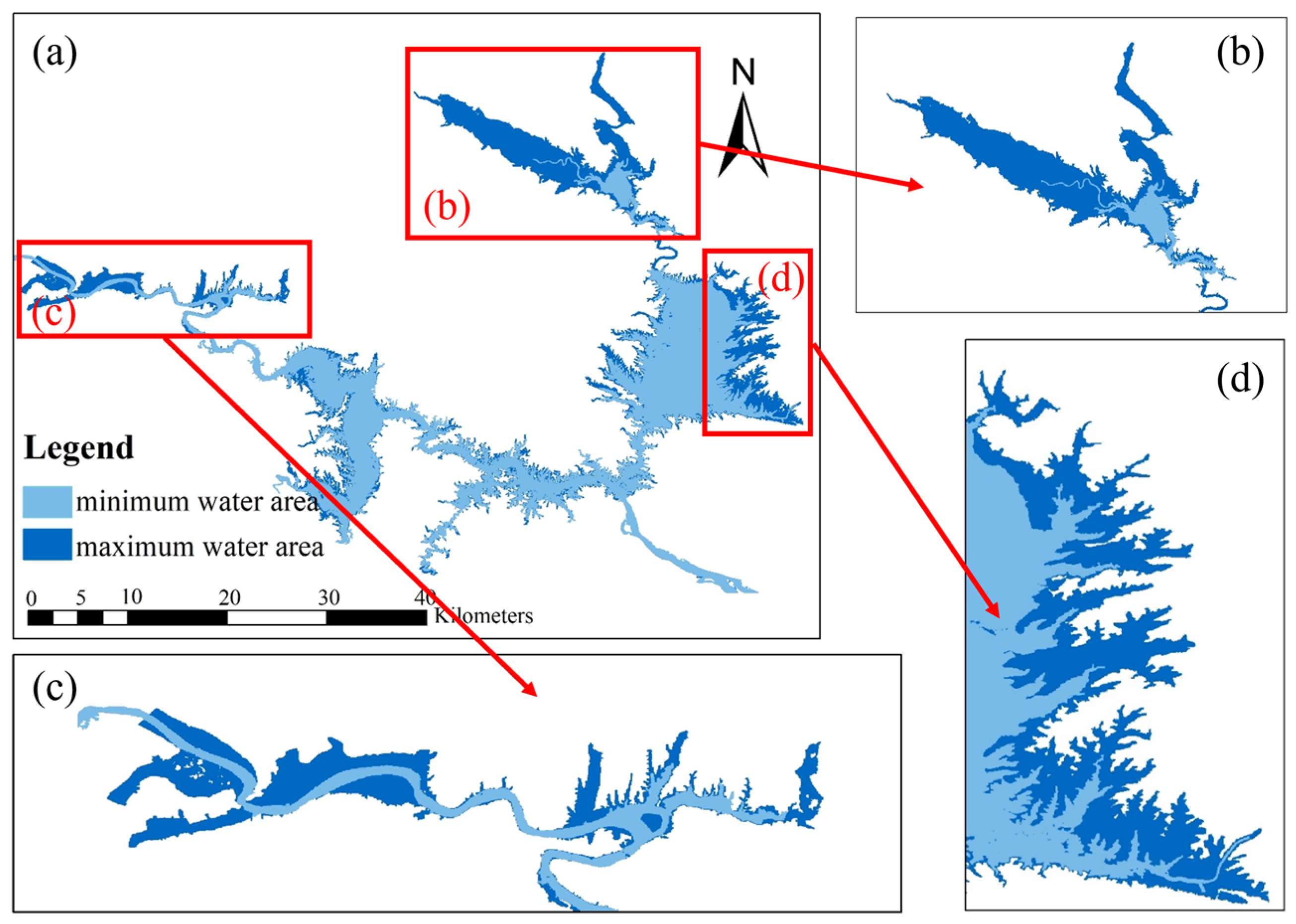
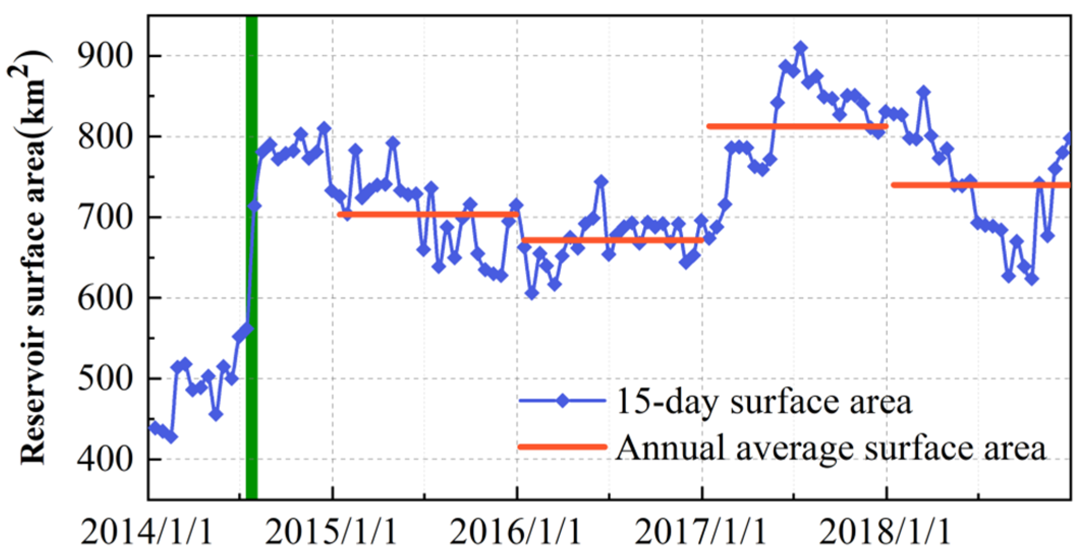
4.1. Estimated Reservoir Surface Area

The study period of 2014–2018 was chosen to showcase the notable variations in the water surface area between the periods before (2014–2015) and after (2015–2018) the dam heightening. However, the evaporation analysis primarily focused on the period after the dam heightening (2015–2018) as it is the present condition. Figure 2 shows the 15-day fluctuations in the water surface area of the DJK Reservoir. In 2014, the water surface area of the reservoir increases significantly fluctuates from 426 km² in early 2014 to 790 km² in September due to the dam heightening. From September 2014 to the end of 2018, the surface area fluctuates between 600 km² and 900 km², with the multi-year average water surface area for the years 2015–2018 being 731.9 km² after the dam heightening. The annual average values of the period 2015–2018 are 703, 671, 813, and 740 km², respectively. During this period, the water area experiences frequent and rapid fluctuations, with the maximum value appearing in July 2017 and the minimum value appearing in January 2016. The fluctuation characteristics of the water surface area in the four years after heightening have no seasonality. In 2015, it shows a downward trend. In 2016, the fluctuation is relatively small around the annual average value. In 2017 and 2018, the fluctuation is large, with the maximum and minimum area differences of 236 km² and 231 km², and experiences clear upward and downward changes, respectively.

Figure 3 presents a 30 m spatial resolution image depicting the maximum and minimum water surface areas of the DJK Reservoir from 2015 to 2018. The minimum water surface area (606 km²) occurs on 30 January 2016, while the maximum water surface area (910 km²) occurs on 15 July 2017. The dark blue area illustrates the range of fluctuations in the water surface area between the maximum and minimum. As shown in Figure 3, notable variations primarily occur in three distinct regions in the eastern, western, and northern parts of the reservoir, respectively. Conversely, minor fluctuations are observed in other areas of the reservoir. The differences between the maximum and minimum water surface areas are 69.6, 51.6, and 143.7 km² in the eastern, western, and northern parts of the reservoir, respectively. The total differences between these three regions accounts for about 87.1% of the total difference in the whole reservoir between the maximum and minimum water surface areas. It is worth noting that the boundary of the water surface is fragmental, which indicates the significance of the spatial resolution in accurate water area estimations.

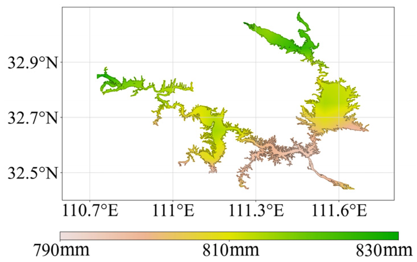
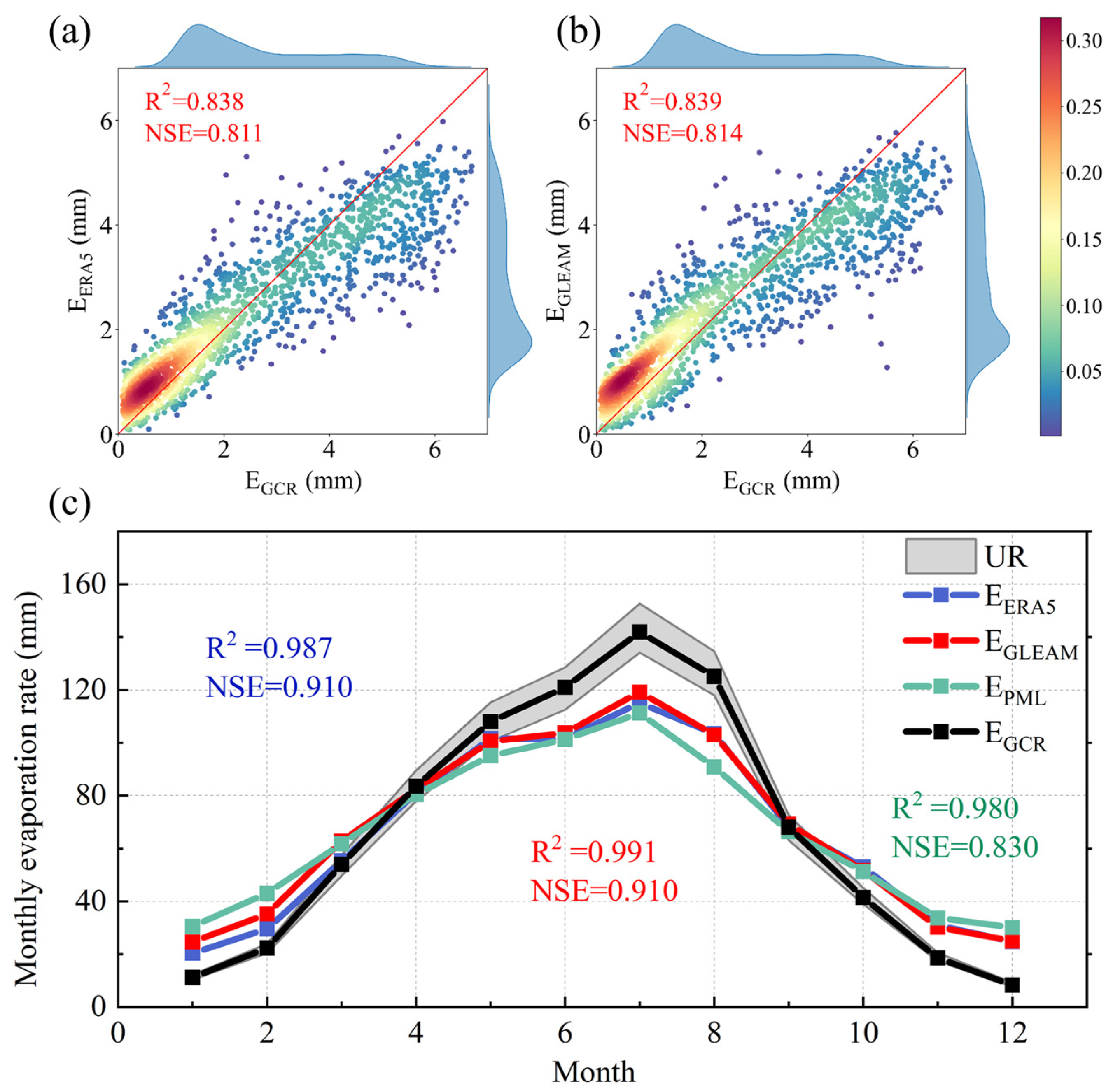
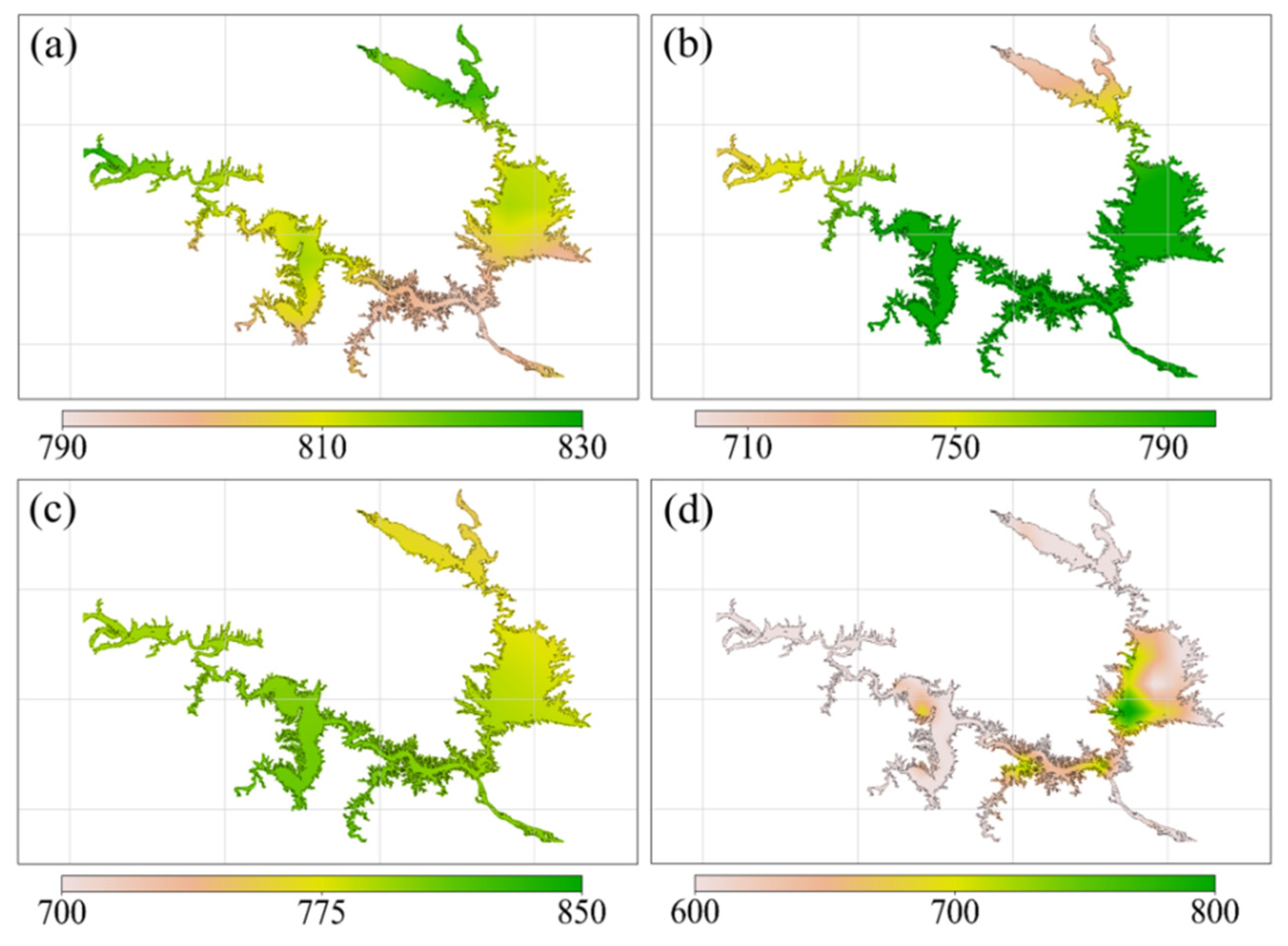
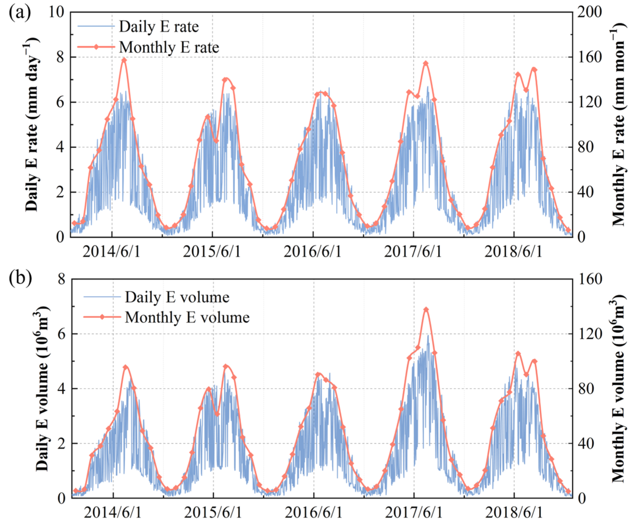
4.2. High Spatiotemporal Estimation of Reservoir Evaporation

Figure 4 shows the daily and monthly evaporation rates (Figure 4a) and volumes (Figure 4b) of the DJK Reservoir from 2014 to 2018. The evaporation rate shows evident seasonal patterns, with higher values observed from May to August and lower values observed from November to February. The daily evaporation rate exhibits rapid and frequent fluctuations, characterized by smaller variations at lower values and larger variations at higher values. Notably, the maximum difference in the evaporation rate between two consecutive days can reach 4.43 mm. Over the period from 2014 to 2018, the average daily evaporation rate is 2.20 mm. The maximum daily evaporation rate of 6.70 mm occurs on 23 July 2017, while the minimum daily evaporation rate of 0.08 mm is observed on 20 December 2014. The average monthly evaporation rate from 2014 to 2018 is 67.0 mm. The highest monthly evaporation rate of 157.3 mm is estimated in July 2014, whereas the lowest monthly evaporation rate of 6.4 mm is observed in December 2018. During the period from May to August in the years 2014 to 2018, the evaporation rates accounts for 62%, 61%, 60%, 64%, and 62% of the annual total evaporation, respectively. The annual evaporation rates of the 5 years are as 794, 763, 772, 835, and 854 mm, respectively. The five-year (2014–2018) average evaporation rate is estimated to be 804 mm.

The evaporation volume exhibits a similar seasonal pattern to the evaporation rate, with higher values observed in the summer and lower values in the winter. The maximum and minimum daily evaporation volumes are observed in July 2017 and December 2014, respectively. The sum of the monthly evaporation volumes for May to August in each year from 2014 to 2018 accounts for 61%, 60%, 61%, 65%, and 61% of the respective year’s total annual evaporation. The five-year (2014–2018) average evaporation volume is 572 million m³. After dam heightening, the mean annual average evaporation volume (2015–2018) is 595 million m³. The annual total evaporation volumes for the years 2014 to 2018 are 480, 538, 527, 698, and 617 million m³, respectively, indicating a larger interannual variation than that of the evaporation rate.

Figure 5 shows the spatial distribution of the multi-year average evaporation rates of the DJK Reservoir after heightening estimated by the GCR with a resolution of 100 m. The multi-year average evaporation rate from 2015 to 2018 is estimated to be 806 mm. Notably, the spatial variation of the evaporation rate in the reservoir is manifested as a decrease from north to south and from west to east. The spatial distribution of the evaporation rates exhibits relatively uniform characteristics, with a difference of 35 mm between the maximum and minimum values. The maximum rate of 828 mm is observed in the northeast and northwest regions, while the minimum rate of 793 mm is observed in the central part of the reservoir.

To validate the suitability of the GCR method for reservoir evaporation estimation, the estimated evaporation rates obtained by the GCR were compared with the datasets derived from the ERA5, GLEAM, and PML in terms of the temporal and spatial consistency. Two performance indices, including the coefficient of determination (R²) and the Nash–Sutcliffe model efficiency coefficient (NSE), were used. Figure 6a,b present the comparison of the daily evaporation rate between the estimated values and the ERA5 and GLEAM from 2014 to 2018. The PML is not compared at the daily time scale due to it being at an 8-day temporal resolution. Both the NSE and R² values are higher than 0.8, indicating the strong consistency of estimated results in this study with other independent estimates. Figure 6c shows the monthly average comparison of the estimated results with the three products from 2014 to 2018 and the uncertainty range (UR) of the GCR. It demonstrates consistent monthly variations among the four datasets. The NSEs of the estimated monthly evaporation rates with the other three products are all above 0.8, and the R² values are all higher than 0.95, indicating a good agreement with the independent estimates. However, it is worth noting that the estimated evaporation rates based on the GCR method are higher than the other three products during the summer months (June to August) and lower during the winter months (November to February).

The downscaled spatial distribution images of the muti-year average ${\mathrm{E}}_{\mathrm{G}\mathrm{C}\mathrm{R}}$, ${\mathrm{E}}_{\mathrm{G}\mathrm{L}\mathrm{E}\mathrm{A}\mathrm{M}}$, ${\mathrm{E}}_{\mathrm{E}\mathrm{R}\mathrm{A}5}$ and ${\mathrm{E}}_{\mathrm{P}\mathrm{M}\mathrm{L}}$ from 2014 to 2018 at a resolution of 100 m are presented in Figure 7. The magnitudes of the multi-year average values are comparable, with values of 790.12, 786.09, 809.05, and 763.04 mm, respectively. However, the spatial pattern of ${\mathrm{E}}_{\mathrm{G}\mathrm{C}\mathrm{R}}$, as depicted in Figure 7a–d, shows inconsistency with the other three evaporation products. The inconsistency of meteorological data may be a primary factor contributing to the spatial disparity.

To verify the reliability of the estimated evaporation volumes, the comparison with the PH method was conducted at a monthly scale as the PH method has been applied at the monthly time scale before. Figure 8 presents the fitting results of the monthly evaporation volumes using the PH and GCR methods from 2014 to 2018. Notably, the evaporation volumes estimated using the PH method are slightly higher than those of the GCR method during the winter (November to January). Both the NSE and R² exceed 0.94 between the monthly results estimated using the PH and GCR methods, indicating high overall consistency.

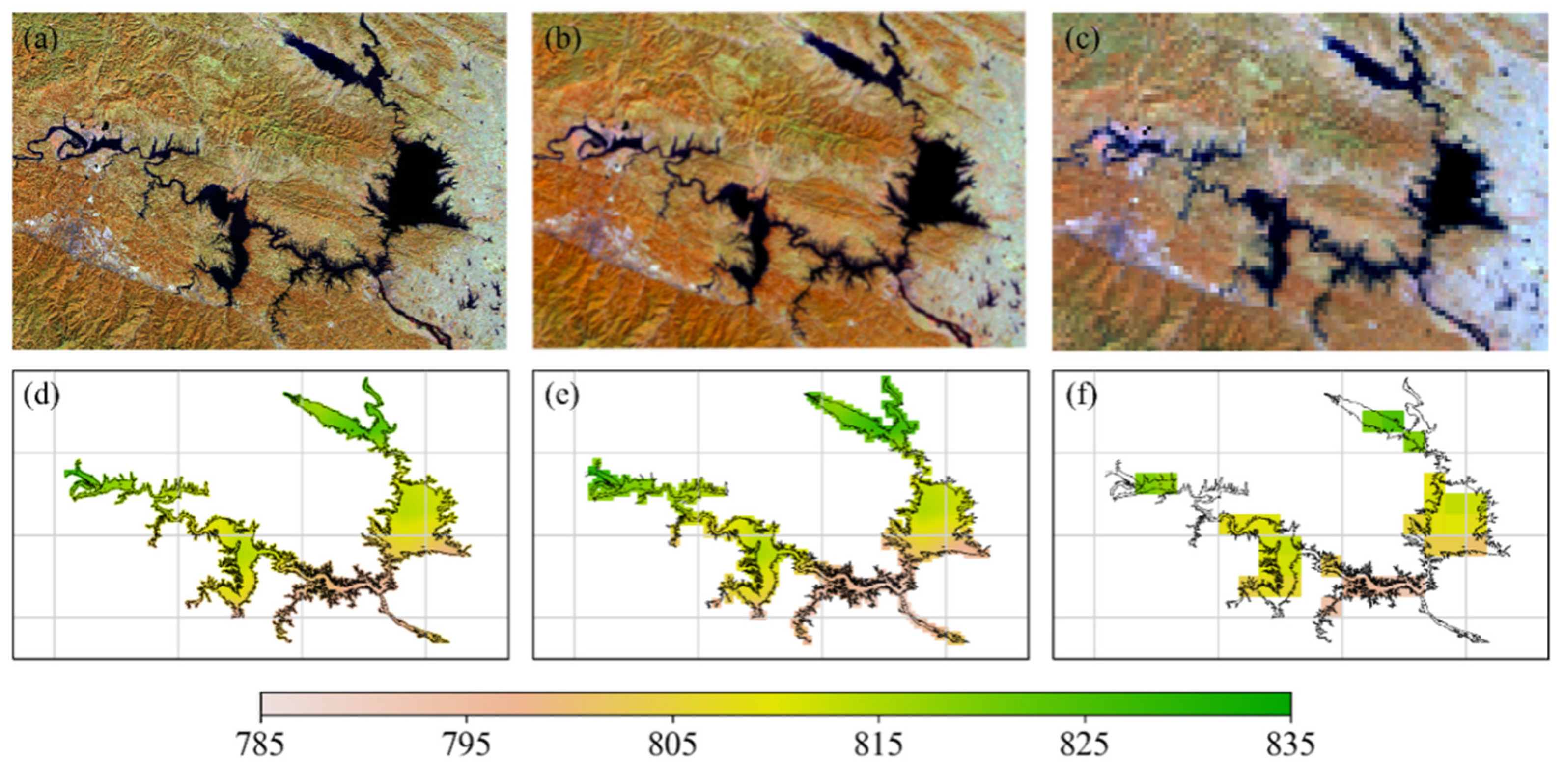
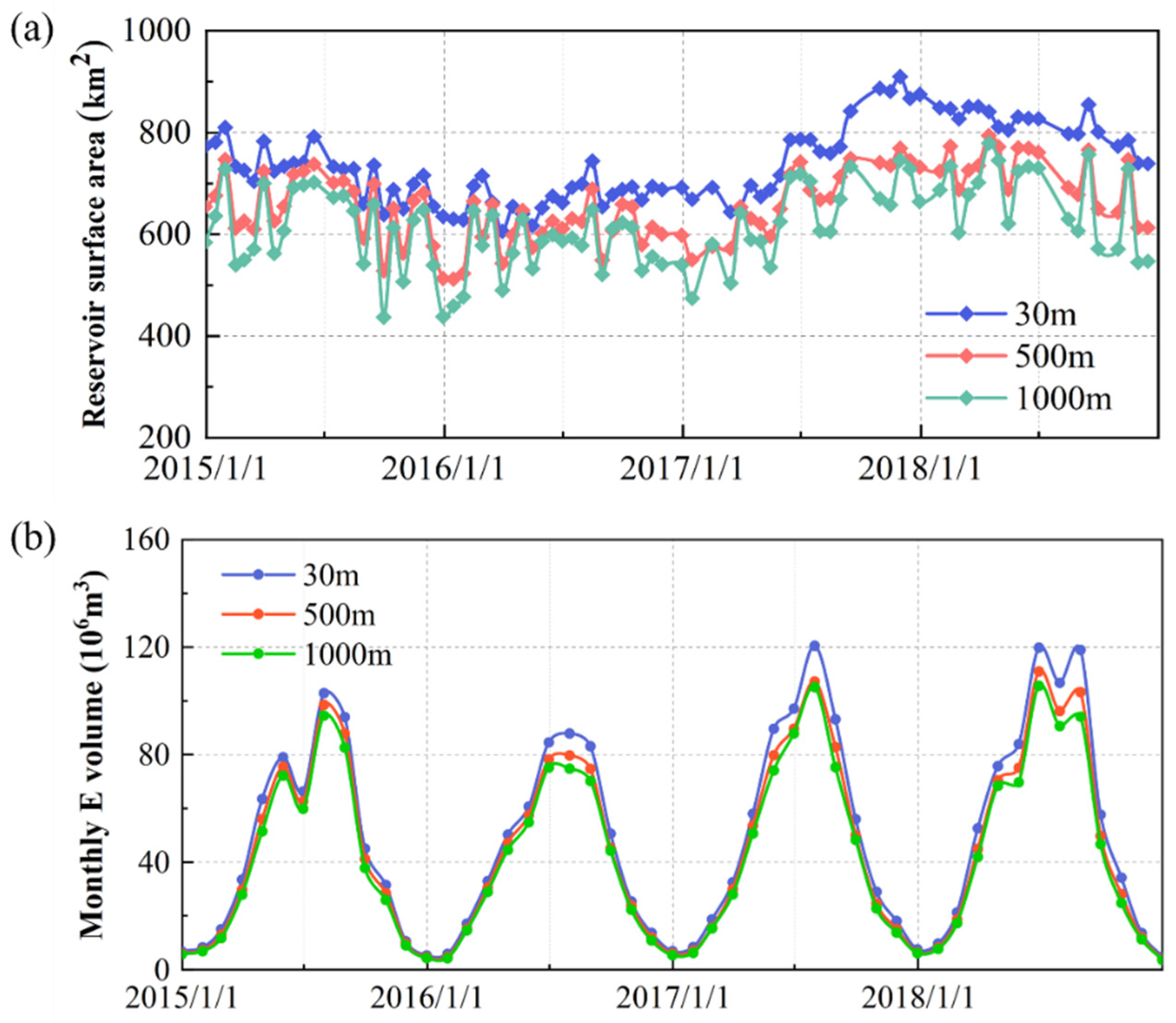
4.3. Influences of Data Resolutions on Evaporation Estimation

Figure 9 shows images of the water surface area of 30 m, 500 m, and 1000 m resolutions and the estimated evaporation rates of 100 m, 1000 m, and 5000 m resolutions. The water surface area image with a resolution of 30 m was obtained using the ESTARFM. The 500 m data was directly derived from the MODIS, while the 1000 m data, due to the lack of direct acquisition, was obtained by upscaling using the GEE reprojection method. There is a significant disparity in the clarity of the water surface area images at different resolutions. Importantly, the image with a resolution of 30 m exhibits clear water–land boundaries, which is a crucial factor influencing water surface area extraction. Notably, high-resolution evaporation rate images display more continuous spatial patterns and mitigate the occurrence of extensive data gaps, as is shown in Figure 9f. As the evaporation rate represents the mean value across all the grid cells within the basin, there is minimal divergence in the evaporation rates at different spatial resolutions, consequently exerting a negligible impact on the evaporation estimation. Therefore, this section solely showcases the impact of the water surface area extracted at different spatial resolutions on the estimation of evaporation. Figure 10a shows the variation in the water surface area extracted at different resolutions, with data acquired every 15 days. Substantial differences exist among the three water surface area datasets. The disparities are primarily concentrated in the years 2017–2018, with the difference range between the 30 m and 500 m resolution data being 0.33 km²–151 km², and between 30 m and 1000 m resolution data ranging from 10 km²–229 km². The higher values are relatively close, while the lower values exhibit significant differences. The average values for the water surface area data at resolutions of 30 m, 500 m, and 1000 m are 734, 662, and 620 km², respectively. The three water surface area datasets (30 m, 500 m, and 1000 m) are used in conjunction with the same climate-forcing data (100 m) to estimate the monthly evaporation volume. Figure 10b demonstrates noticeable differences among the three estimated evaporation volumes, primarily concentrated in the summer season, with little difference in winter. The annual average evaporation volumes at the three different spatial resolutions are 556, 514, and 488 million m³, respectively. Compared to the results at the 100 m resolution, the estimated mean annual evaporation volume is 9% and 14% smaller at the 500 m and 1000 m resolutions, respectively. The use of reprojection in obtaining the 1000 m water surface area data may have a certain impact on the results. However, the significant differences in the evaporation estimation results caused by data of different resolutions still persist.

5. Discussion

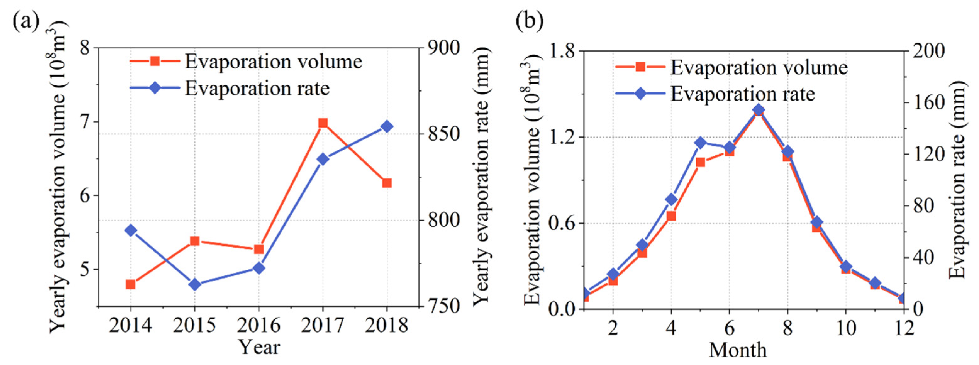
5.1. Attribution of Interannual Variability of Reservoir Evaporation Volume

Most existing studies on evaporation estimation primarily focus on evaporation rates, but relying solely on evaporation rates may not offer a comprehensive depiction of the evaporation losses from reservoirs. As shown in Figure 11a, the evaporation rates and volumes exhibit apparently different inter-annual variations. Except for the variations from 2016 to 2017, the changes in the remaining three between-year variations are the opposite. Figure 11b displays the inconsistent variations in the monthly evaporation rates and volumes in 2017, particularly during May and June. This indicates that evaporation rates alone are insufficient for assessing evaporation losses in reservoirs. To quantify the impact of the water surface area on the evaporation volume variations, a detrending method [65,66] was employed to estimate the contribution. The results indicate that the water surface area and climate forcing account for 95.8% and 4.2% of the variation, respectively. It is found that the water surface area makes the dominant contribution, consistent with the previous analysis [67]. According to the contribution analysis method, the larger the water surface area, the greater its impact on the evaporation volume, while the contribution of meteorological factors becomes smaller. In the case of the DJK Reservoir, a large reservoir with a water surface area of 708 km², meteorological factors exert minimal influence on evaporation. Nevertheless, the results demonstrate the importance of considering the water surface area as a crucial factor in quantifying the evaporation loss of the reservoir. In reality, the water surface area of reservoirs often undergoes significant dynamic changes in the short term for multiple reservoir operation purposes, highlighting the importance of obtaining high temporal resolution water surface area data for accurately estimating evaporation losses in reservoirs.

5.2. Uncertainty Analysis

The uncertainty associated with the ESTARFM algorithm primarily comes from the selection of similar image pairs. Due to the high requirements of image pairs for the fusion, only 18 pairs of similar images were identified between 2014 and 2018. Consequently, when predicting an image at a specific moment, the significant intervals between the preceding and succeeding time periods may result in an inability to accurately capture the irregular variations in the reservoir, resulting in uncertainty that is challenging to calculate and analyze.

The generalized complementary relationship (GCR), introduced by Brutsaert [51], has been validated and successfully applied in various global climates and landscapes. The preliminary evidence of the comparison with three evaporation products demonstrates the applicability of the GCR method for water surface evaporation estimation. However, due to the lack of actual measured values for comparison, further analysis of the uncertainty of the GCR method is required. The influence of the parameter ${\alpha }_c$ on evaporation rate estimation using the GCR was analyzed by arbitrarily varying its value within ±5% and running over 100 times. This 5% adjustment was compared to variable uncertainties, as depicted in the uncertainty range (UR) of the GCR shown in Figure 6c. The maximum UR at monthly scale is 18.5 mm in July, and the minimum is 1.5 mm in December. A 5% variation in ${\alpha }_c$ results in a 5.7% change in the evaporation rate.

6. Conclusions

This study proposes a new method to perform high spatiotemporal estimation of reservoir evaporation losses by integrating remote sensing and evaporation models. By applying the method to the DJK Reservoir, the high spatial (30 m) and temporal (daily) water surface area was derived using the ESTARFM, and the high spatial (100 m) and temporal (daily) evaporation rate was estimated using the GCR. The evaporation losses were subsequently estimated as the product of the surface area and evaporation rate. The magnitudes and spatiotemporal variations of the reservoir surface area, evaporation rate, and reservoir evaporation volume were analyzed. Different data resolution has a great influence on the estimation of the evaporation volume, and the difference between low-resolution and high-resolution data reaches 14%. Compared with the other three evaporation products and methods, the applicability of the GCR in estimating water surface evaporation is verified. This study highlights the importance of using the evaporation volume rather than relying solely on the evaporation rate to assess the evaporation losses from reservoirs. These findings enhance the understanding of the evaporation process from the reservoir and provide a valuable basis for optimizing the water resource management of the reservoir.

References

1. Grossman, R.L.; Friedrich, K.; Huntington, J.; Blanken, P.D.; Lenters, J.; Holman, K.D.; Gochis, D.; Livneh, B.; Prairie, J.; Skeie, E.; et al. Reservoir Evaporation in the Western United States: Current Science, Challenges, and Future Needs. Bull. Am. Meteorol. Soc. 2018, 99, 167–187. [Google Scholar] [CrossRef]
2. Dai, A.; Zhao, T.; Chen, J. Climate change and drought: A precipitation and evaporation perspective. Curr. Clim. Chang. Rep. 2018, 4, 301–312. [Google Scholar] [CrossRef]
3. Wang, Q.; Deng, H.; Jian, J. Hydrological Processes under Climate Change and Human Activities: Status and Challenges. Water 2023, 15, 4164. [Google Scholar] [CrossRef]
4. Zhang, H.; Gorelick, S.M.; Zimba, P.V.; Zhang, X. A remote sensing method for estimating regional reservoir area and evaporative loss. J. Hydrol. 2017, 555, 213–227. [Google Scholar] [CrossRef]
5. Zhan, S.; Song, C.; Wang, J.; Sheng, Y.; Quan, J. A global assessment of terrestrial evapotranspiration increase due to surface water area change. Earth’s Future 2019, 7, 266–282. [Google Scholar] [CrossRef] [PubMed]
6. Rodrigues, C.M.; Moreira, M.; Guimarães, R.C.; Potes, M. Reservoir evaporation in a Mediterranean climate: Comparing direct methods in Alqueva Reservoir, Portugal. Hydrol. Earth Syst. Sci. 2020, 24, 5973–5984. [Google Scholar] [CrossRef]
7. Zhou, L.; Cheng, L.; Qin, S.; Mai, Y.; Lu, M. Estimation of Urban Evapotranspiration at High Spatiotemporal Resolution and Considering Flux Footprints. Remote Sens. 2023, 15, 1327. [Google Scholar] [CrossRef]
8. Zhao, G.; Gao, H.; Cai, X. Estimating lake temperature profile and evaporation losses by leveraging MODIS LST data. Remote Sens. Environ. 2020, 251, 112104. [Google Scholar] [CrossRef]
9. Gallego-Elvira, B.; Baille, A.; Martin-Gorriz, B.; Maestre-Valero, J.; Martinez-Alvarez, V. Evaluation of evaporation estimation methods for a covered reservoir in a semi-arid climate (south-eastern Spain). J. Hydrol. 2012, 458, 59–67. [Google Scholar] [CrossRef]
10. Majidi, M.; Alizadeh, A.; Farid, A.; Vazifedoust, M. Estimating Evaporation from Lakes and Reservoirs under Limited Data Condition in a Semi-Arid Region. Water Resour. Manag. 2015, 29, 3711–3733. [Google Scholar] [CrossRef]
11. McVicar, T.R.; Roderick, M.L.; Donohue, R.J.; Li, L.T.; Van Niel, T.G.; Thomas, A.; Grieser, J.; Jhajharia, D.; Himri, Y.; Mahowald, N.M. Global review and synthesis of trends in observed terrestrial near-surface wind speeds: Implications for evaporation. J. Hydrol. 2012, 416, 182–205. [Google Scholar] [CrossRef]
12. Vinukollu, R.K.; Wood, E.F.; Ferguson, C.R.; Fisher, J.B. Global estimates of evapotranspiration for climate studies using multi-sensor remote sensing data: Evaluation of three process-based approaches. Remote Sens. Environ. 2011, 115, 801–823. [Google Scholar] [CrossRef]
13. Pan, S.; Pan, N.; Tian, H.; Friedlingstein, P.; Sitch, S.; Shi, H.; Arora, V.K.; Haverd, V.; Jain, A.K.; Kato, E. Evaluation of global terrestrial evapotranspiration using state-of-the-art approaches in remote sensing, machine learning and land surface modeling. Hydrol. Earth Syst. Sci. 2020, 24, 1485–1509. [Google Scholar] [CrossRef]
14. Wang, Y.; Merlin, O.; Zhu, G.; Zhang, K. A physically based method for soil evaporation estimation by revisiting the soil drying process. Water Resour. Res. 2019, 55, 9092–9110. [Google Scholar] [CrossRef]
15. Althoff, D.; Rodrigues, L.N.; da Silva, D.D. Impacts of climate change on the evaporation and availability of water in small reservoirs in the Brazilian savannah. Clim. Chang. 2020, 159, 215–232. [Google Scholar] [CrossRef]
16. Chen, F.; Mitchell, K.; Schaake, J.; Xue, Y.; Pan, H.L.; Koren, V.; Duan, Q.Y.; Ek, M.; Betts, A. Modeling of land surface evaporation by four schemes and comparison with FIFE observations. J. Geophys. Res. Atmos. 1996, 101, 7251–7268. [Google Scholar] [CrossRef]
17. Zhao, G.; Gao, H. Estimating reservoir evaporation losses for the United States: Fusing remote sensing and modeling approaches. Remote Sens. Environ. 2019, 226, 109–124. [Google Scholar] [CrossRef]
18. Cheng, L.; Xu, Z.; Wang, D.; Cai, X. Assessing interannual variability of evapotranspiration at the catchment scale using satellite-based evapotranspiration data sets. Water Resour. Res. 2011, 47. [Google Scholar] [CrossRef]
19. Khandelwal, A.; Karpatne, A.; Marlier, M.E.; Kim, J.; Lettenmaier, D.P.; Kumar, V. An approach for global monitoring of surface water extent variations in reservoirs using MODIS data. Remote Sens. Environ. 2017, 202, 113–128. [Google Scholar] [CrossRef]
20. Huang, S.; Li, J.; Xu, M. Water surface variations monitoring and flood hazard analysis in Dongting Lake area using long-term Terra/MODIS data time series. Nat. Hazards 2012, 62, 93–100. [Google Scholar] [CrossRef]
21. Li, X.; Ling, F.; Foody, G.M.; Boyd, D.S.; Jiang, L.; Zhang, Y.; Zhou, P.; Wang, Y.; Chen, R.; Du, Y. Monitoring high spatiotemporal water dynamics by fusing MODIS, Landsat, water occurrence data and DEM. Remote Sens. Environ. 2021, 265, 112680. [Google Scholar] [CrossRef]
22. Xia, H.; Zhao, J.; Qin, Y.; Yang, J.; Cui, Y.; Song, H.; Ma, L.; Jin, N.; Meng, Q. Changes in Water Surface Area during 1989–2017 in the Huai River Basin using Landsat Data and Google Earth Engine. Remote Sens. 2019, 11, 1824. [Google Scholar] [CrossRef]
23. Chang, L.; Cheng, L.; Huang, C.; Qin, S.; Fu, C.; Li, S. Extracting urban water bodies from Landsat imagery based on mNDWI and HSV transformation. Remote Sens. 2022, 14, 5785. [Google Scholar] [CrossRef]
24. Zeng, J.; Zhou, T.; Wang, Q.; Xu, Y.; Lin, Q.; Zhang, Y.; Wu, X.; Zhang, J.; Liu, X. Spatial patterns of China’s carbon sinks estimated from the fusion of remote sensing and field-observed net primary productivity and heterotrophic respiration. Ecol. Inform. 2023, 76, 102152. [Google Scholar] [CrossRef]
25. Gao, F.; Anderson, M.C.; Zhang, X.; Yang, Z.; Alfieri, J.G.; Kustas, W.P.; Mueller, R.; Johnson, D.M.; Prueger, J.H. Toward mapping crop progress at field scales through fusion of Landsat and MODIS imagery. Remote Sens. Environ. 2017, 188, 9–25. [Google Scholar] [CrossRef]
26. Zhao, Y.; Huang, B.; Song, H. A robust adaptive spatial and temporal image fusion model for complex land surface changes. Remote Sens. Environ. 2018, 208, 42–62. [Google Scholar] [CrossRef]
27. Gao, F.; Masek, J.; Schwaller, M.; Hall, F. On the blending of the Landsat and MODIS surface reflectance: Predicting daily Landsat surface reflectance. IEEE Trans. Geosci. Remote Sens. 2006, 44, 2207–2218. [Google Scholar]
28. Zhu, X.; Chen, J.; Gao, F.; Chen, X.; Masek, J.G. An enhanced spatial and temporal adaptive reflectance fusion model for complex heterogeneous regions. Remote Sens. Environ. 2010, 114, 2610–2623. [Google Scholar] [CrossRef]
29. Ma, J.; Zhang, W.; Marinoni, A.; Gao, L.; Zhang, B. Performance assessment of ESTARFM with different similar-pixel identification schemes. J. Appl. Remote Sens. 2018, 12, 025017. [Google Scholar] [CrossRef]
30. Zhu, X.; Cai, F.; Tian, J.; Williams, T. Spatiotemporal Fusion of Multisource Remote Sensing Data: Literature Survey, Taxonomy, Principles, Applications, and Future Directions. Remote Sens. 2018, 10, 527. [Google Scholar] [CrossRef]
31. Kohler, M.A.; Nordenson, T.J.; Fox, W. Evaporation from Pans and Lakes; US Government Printing Office: Benicia, CA, USA, 1955; Volume 30.
32. Blanken, P.D.; Rouse, W.R.; Culf, A.D.; Spence, C.; Boudreau, L.D.; Jasper, J.N.; Kochtubajda, B.; Schertzer, W.M.; Marsh, P.; Verseghy, D. Eddy covariance measurements of evaporation from Great Slave lake, Northwest Territories, Canada. Water Resour. Res. 2000, 36, 1069–1077. [Google Scholar] [CrossRef]
33. Finch, J.; Calver, A. Methods for the Quantification of Evaporation from Lakes; World Meteorological Organization’s Commission for Hydrology: Geneva, Switzerland, 2008. [Google Scholar]
34. Brutsaert, W. Evaporation into the Atmosphere: Theory, History and Applications; Springer Science & Business Media: Berlin, Germany, 2013; Volume 1. [Google Scholar]
35. Penman, H.L. Natural evaporation from open water, bare soil and grass. Proceedings of the Royal Society of London. Ser. A Math. Phys. Sci. 1948, 193, 120–145. [Google Scholar]
36. Penman, H. Evaporation: An introductory survey. Neth. J. Agric. Sci. 1956, 4, 9–29. [Google Scholar] [CrossRef]
37. Pham, T.T.; Mai, T.D.; Pham, T.D.; Hoang, M.T.; Nguyen, M.K.; Pham, T.T. Industrial water mass balance as a tool for water management in industrial parks. Water Resour. Ind. 2016, 13, 14–21. [Google Scholar] [CrossRef]
38. Stannard, D.; Gannett, M.; Polette, D.; Cameron, J.; Waibel, M.; Spears, J. Evapotranspiration from marsh and open-water sites at Upper Klamath Lake. Oregon 2008, 2010, 2013. [Google Scholar]
39. Wang, K.; Dickinson, R.E. A review of global terrestrial evapotranspiration: Observation, modeling, climatology, and climatic variability. Rev. Geophys. 2012, 50. [Google Scholar] [CrossRef]
40. Morton, F.I. Operational estimates of areal evapotranspiration and their significance to the science and practice of hydrology. J. Hydrol. 1983, 66, 1–76. [Google Scholar] [CrossRef]
41. Brutsaert, W.; Cheng, L.; Zhang, L. Spatial Distribution of Global Landscape Evaporation in the Early Twenty-First Century by Means of a Generalized Complementary Approach. J. Hydrometeorol. 2020, 21, 287–298. [Google Scholar] [CrossRef]
42. Bouchet, R. Actual and potential evapotranspiration, climatic significance. IAHS Publ. 1963, 62, 134–142. [Google Scholar]
43. Dimitriadou, S.; Nikolakopoulos, K.G. Evapotranspiration trends and interactions in light of the anthropogenic footprint and the climate crisis: A review. Hydrology 2021, 8, 163. [Google Scholar] [CrossRef]
44. Lei, X.; Cheng, L.; Ye, L.; Zhang, L.; KIM, J.S.; Qin, S.; Liu, P. Integration of the generalized complementary relationship into a lumped hydrological model for improving water balance partitioning: A case study with the Xinanjiang model. J. Hydrol. 2023, 621, 129569. [Google Scholar] [CrossRef]
45. Lei, X.; Cheng, L.; Zhang, L.; Cheng, S.; Qin, S.; Liu, P. Improving the Applicability of Lumped Hydrological Models by Integrating the Generalized Complementary Relationship. Water Resour. Res. 2024, 60, e2023WR035567. [Google Scholar] [CrossRef]
46. Zhang, L.; Cheng, L.; Brutsaert, W. Estimation of land surface evaporation using a generalized nonlinear complementary relationship. J. Geophys. Res. Atmos. 2017, 122, 1475–1487. [Google Scholar] [CrossRef]
47. Bonnema, M.; David, C.H.; Frasson, R.P.d.M.; Oaida, C.; Yun, S.H. The Global Surface Area Variations of Lakes and Reservoirs as Seen From Satellite Remote Sensing. Geophys. Res. Lett. 2022, 49, e2022GL098987. [Google Scholar] [CrossRef]
48. Ramírez, J.A.; Hobbins, M.T.; Brown, T.C. Observational evidence of the complementary relationship in regional evaporation lends strong support for Bouchet’s hypothesis. Geophys. Res. Lett. 2005, 32, L15401. [Google Scholar] [CrossRef]
49. Liu, X.; Liu, C.; Brutsaert, W. Investigation of a generalized nonlinear form of the complementary principle for evaporation estimation. J. Geophys. Res. Atmos. 2018, 123, 3933–3942. [Google Scholar] [CrossRef]
50. Han, S.; Tian, F. A review of the complementary principle of evaporation: From the original linear relationship to generalized nonlinear functions. Hydrol. Earth Syst. Sci. 2020, 24, 2269–2285. [Google Scholar] [CrossRef]
51. Brutsaert, W. A generalized complementary principle with physical constraints for land-surface evaporation. Water Resour. Res. 2015, 51, 8087–8093. [Google Scholar] [CrossRef]
52. Cogley, J.G. The albedo of water as a function of latitude. Mon. Weather Rev. 1979, 107, 775–781. [Google Scholar] [CrossRef]
53. Kahler, D.M.; Brutsaert, W. Complementary relationship between daily evaporation in the environment and pan evaporation. Water Resour. Res. 2006, 42. [Google Scholar] [CrossRef]
54. Brutsaert, W. Use of pan evaporation to estimate terrestrial evaporation trends: The case of the Tibetan Plateau. Water Resour. Res. 2013, 49, 3054–3058. [Google Scholar] [CrossRef]
55. Brutsaert, W.; Stricker, H. An advection-aridity approach to estimate actual regional evapotranspiration. Water Resour. Res. 1979, 15, 443–450. [Google Scholar] [CrossRef]
56. Zhao, J.; Li, H.; Cai, X.; Chen, F.; Wang, L.; Yu, D. Long-term (2002–2017) impacts of Danjiangkou dam on thermal regimes of downstream Han River (China) using Landsat thermal infrared imagery. J. Hydrol. 2020, 589, 125135. [Google Scholar] [CrossRef]
57. Chen, M.; Jin, X.; Liu, Y.; Guo, L.; Ma, Y.; Guo, C.; Wang, F.; Xu, J. Human activities induce potential aquatic threats of micropollutants in Danjiangkou Reservoir, the largest artificial freshwater lake in Asia. Sci. Total Environ. 2022, 850, 157843. [Google Scholar] [CrossRef] [PubMed]
58. Li, S.; Zhang, Q. Partial pressure of CO2 and CO2 emission in a monsoon-driven hydroelectric reservoir (Danjiangkou Reservoir), China. Ecol. Eng. 2014, 71, 401–414. [Google Scholar] [CrossRef]
59. Zhang, C.; Duan, Q.; Yeh, P.J.F.; Pan, Y.; Gong, H.; Gong, W.; Di, Z.; Lei, X.; Liao, W.; Huang, Z. The effectiveness of the South-to-North Water Diversion Middle Route Project on water delivery and groundwater recovery in North China Plain. Water Resour. Res. 2020, 56, e2019WR026759. [Google Scholar] [CrossRef]
60. Du, C.; Ren, X.; Zhang, L.; Xu, M.; Wang, X.; Zhuang, Y.; Du, Y. Adsorption Characteristics of Phosphorus onto Soils from Water Level Fluctuation Zones of the Danjiangkou Reservoir. CLEAN—Soil Air Water 2016, 44, 975–983. [Google Scholar] [CrossRef]
61. He, J.; Yang, K.; Tang, W.; Lu, H.; Qin, J.; Chen, Y.; Li, X. The first high-resolution meteorological forcing dataset for land process studies over China. Sci. Data 2020, 7, 25. [Google Scholar] [CrossRef] [PubMed]
62. Miralles, D.G.; Holmes, T.; De Jeu, R.; Gash, J.; Meesters, A.; Dolman, A. Global land-surface evaporation estimated from satellite-based observations. Hydrol. Earth Syst. Sci. 2011, 15, 453–469. [Google Scholar] [CrossRef]
63. Bell, B.; Hersbach, H.; Simmons, A.; Berrisford, P.; Dahlgren, P.; Horányi, A.; Muñoz-Sabater, J.; Nicolas, J.; Radu, R.; Schepers, D. The ERA5 global reanalysis: Preliminary extension to 1950. Q. J. R. Meteorol. Soc. 2021, 147, 4186–4227. [Google Scholar] [CrossRef]
64. Zhang, Y.; Kong, D.; Gan, R.; Chiew, F.H.; McVicar, T.R.; Zhang, Q.; Yang, Y. Coupled estimation of 500 m and 8-day resolution global evapotranspiration and gross primary production in 2002–2017. Remote Sens. Environ. 2019, 222, 165–182. [Google Scholar] [CrossRef]
65. Mao, Y.; Nijssen, B.; Lettenmaier, D.P. Is climate change implicated in the 2013-2014 California drought? A hydrologic perspective. Geophys. Res. Lett. 2015, 42, 2805–2813. [Google Scholar] [CrossRef]
66. Zhang, J.; Sun, F.; Xu, J.; Chen, Y.; Sang, Y.F.; Liu, C. Dependence of trends in and sensitivity of drought over China (1961–2013) on potential evaporation model. Geophys. Res. Lett. 2016, 43, 206–213. [Google Scholar] [CrossRef]
67. Tian, W.; Liu, X.; Wang, K.; Bai, P.; Liu, C. Estimation of reservoir evaporation losses for China. J. Hydrol. 2021, 596, 126142. [Google Scholar] [CrossRef]
Figure 1. Elevation and water surface distribution map of the Danjiangkou (DJK) Reservoir.
Remotesensing 16 01320 g001
Figure 2. The variation in the 15-day water surface area of the DJK Reservoir (2014–2018). The green line represents the heightening event; the red line represents the annual average surface area of each year.
Remotesensing 16 01320 g002
Figure 3. (a) Maximum and minimum water surface area of the DJK Reservoir. Subplots (bd) depict regions with significant water surface area variation in the northern, western, and eastern parts.
Remotesensing 16 01320 g003
Figure 4. Daily and monthly variation in the (a) evaporation rates and (b) volumes of the DJK Reservoir (2014–2018).
Remotesensing 16 01320 g004
Figure 5. Spatial variation in the annual average evaporation rates of DKJ reservoir estimated by the GCR.
Remotesensing 16 01320 g005
Figure 6. Comparison of the daily evaporation rates (a) between EGCR and EERA5, and (b) between EGCR and EGLEAM. (c) Comparison of the monthly average evaporation rates of different estimates.
Remotesensing 16 01320 g006
Figure 7. Spatial consistency between the GCR and evaporation products (2014–2018). (a) Spatial distribution of the annual average evaporation rates estimated by the GCR. Subplots (bd) depict the spatial distribution of the annual average evaporation rates obtained from the GLEAM, ERA5, and PML datasets.
Remotesensing 16 01320 g007
Figure 8. Comparison of the monthly average evaporation volume estimated by the GCR (VEGCR) and PH (VEPH).
Remotesensing 16 01320 g008
Figure 9. Comparison of the water surface area and estimated annual evaporation rate at different spatial resolutions for the DJK Reservoir. Subplots (ac) show images of the water surface area at 30 m, 500 m, and 1000 m resolutions, respectively; subplots (df) illustrate the spatial distribution of the annual average evaporation rate at 100 m, 1000 m, and 5000 m resolutions, respectively.
Remotesensing 16 01320 g009
Figure 10. (a) The 15-day water surface area and (b) monthly evaporation volumes of three different spatial resolutions for the DJK Reservoir (2015–2018).
Remotesensing 16 01320 g010
Figure 11. (a) Annual variation in the evaporation rates and volumes (2014–2018). (b) Monthly variation in the evaporation rates and volumes in 2017.
Remotesensing 16 01320 g011
Disclaimer/Publisher’s Note: The statements, opinions and data contained in all publications are solely those of the individual author(s) and contributor(s) and not of MDPI and/or the editor(s). MDPI and/or the editor(s) disclaim responsibility for any injury to people or property resulting from any ideas, methods, instructions or products referred to in the content.