
Real-Time LEO Satellite Clocks Based on Near-Real-Time Clock Determination with Ultra-Short-Term Prediction
 , , , and
Abstract
:1. Introduction
2. Method
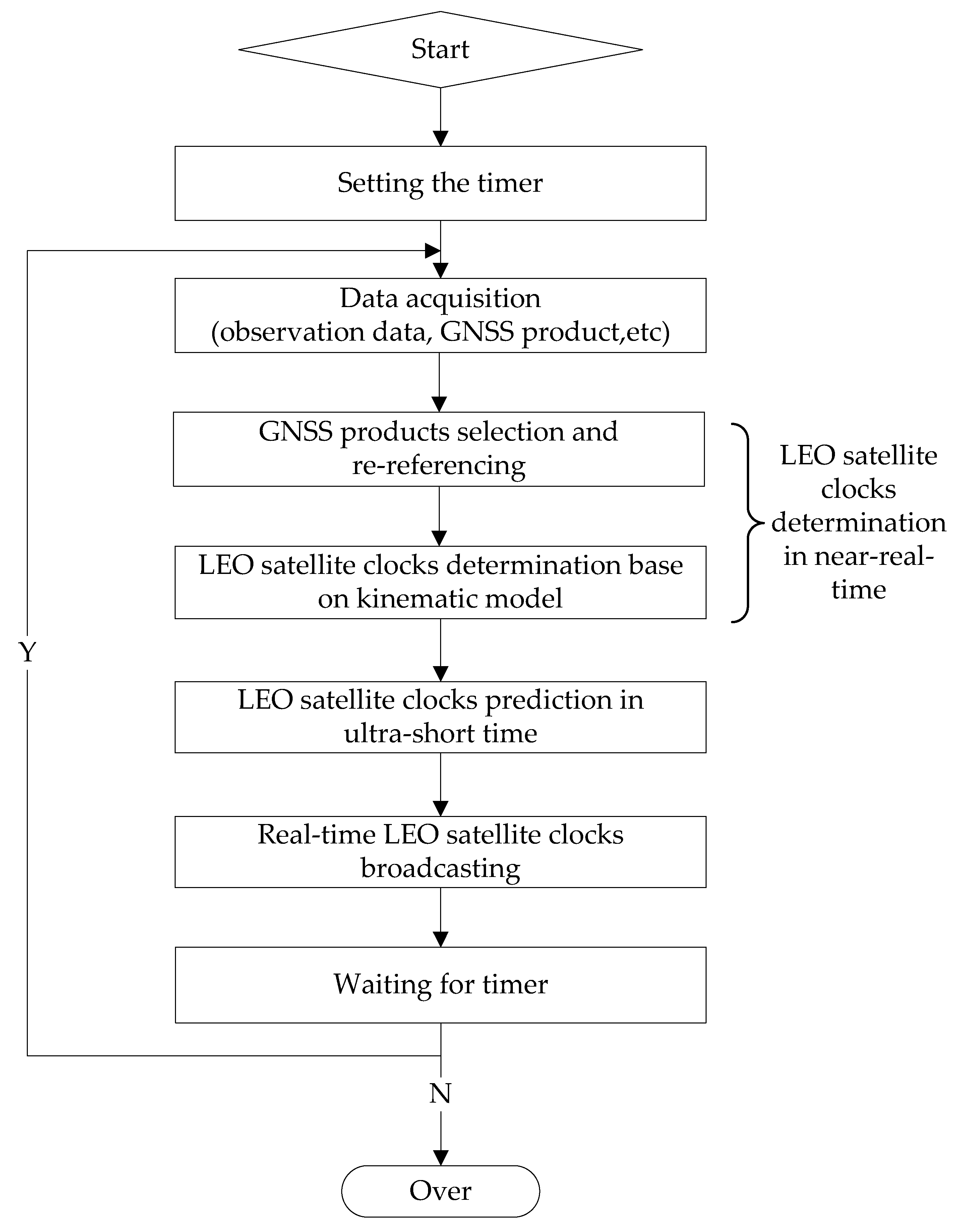
- (1)
- Set a timer and loop through the steps (2)–(4);
- (2)
- Use real-time GNSS orbits, clocks and LEO satellite on-board GNSS observation to determine the near-real-time LEO satellite clocks based on the kinematic model, including GNSS product selection and the clock re-referencing;
- (3)
- Predict the LEO satellite clocks in the ultra-short term, ensuring that users obtain LEO satellite clock products in real time;
- (4)
- Broadcast the low-order polynomial parameters to users at regular intervals.
2.1. LEO Satellite Clock Determination in Near-Real-Time
- (1)
- Analyze the availability and continuity of each real-time product over a past period.
- (2)
- (3)
- Based on the results of the first two steps, identify a set of optional real-time GNSS products and establish an initial ranking. The ranking list is updated on a daily basis.
- (4)
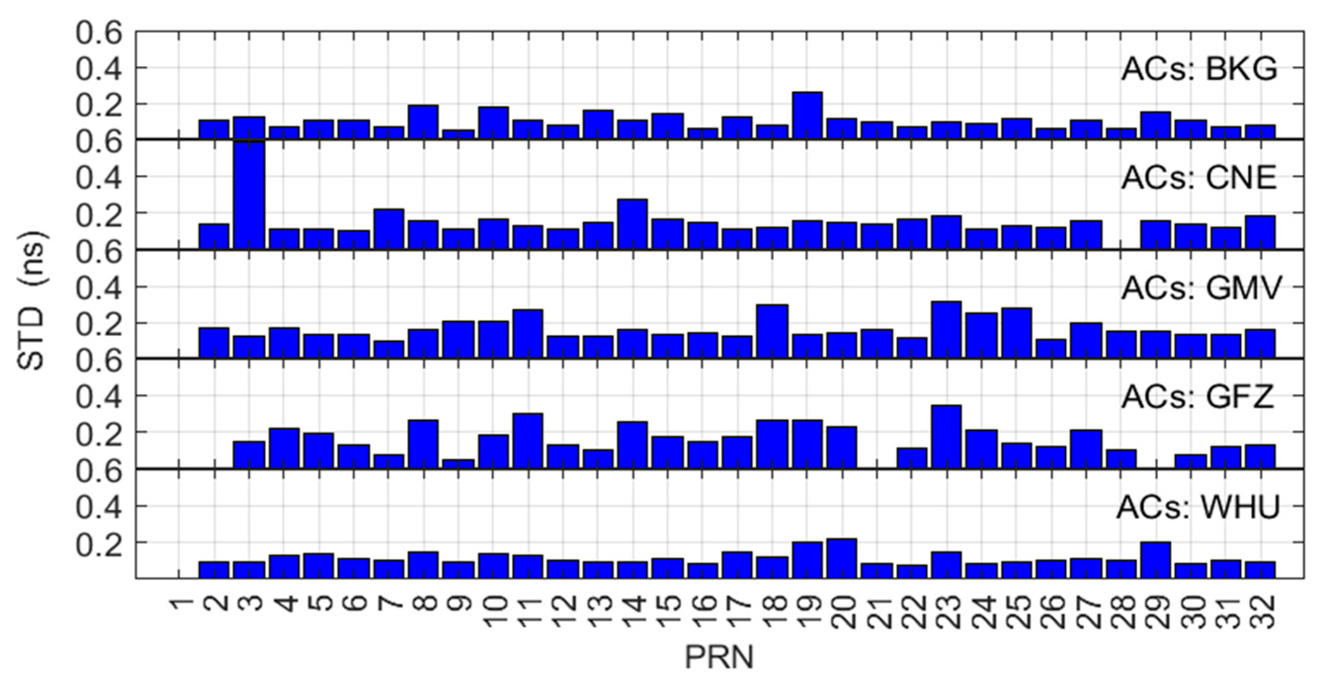
- Upon each processing round, conduct an assessment of the availability/continuity of the real-time products of GNSS satellites in the corresponding processing period. For those passing the pre-defined thresholds for availability and continuity, select the real-time GNSS products according to the ranking list, so that real-time GNSS products with both good completeness and precision can be used for the real-time determination of LEO satellite clocks.
- (1)
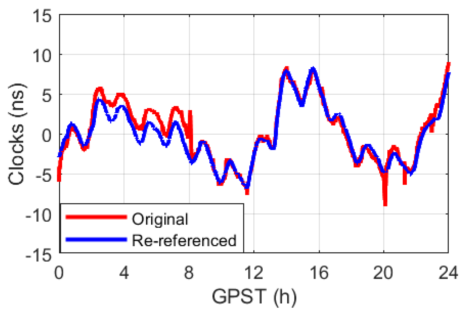
- Inconsistent time references for LEO satellite clocks are determined in each session. This is caused by the different time references of different real-time GNSS satellite clocks provided by different analysis centers.
- (2)
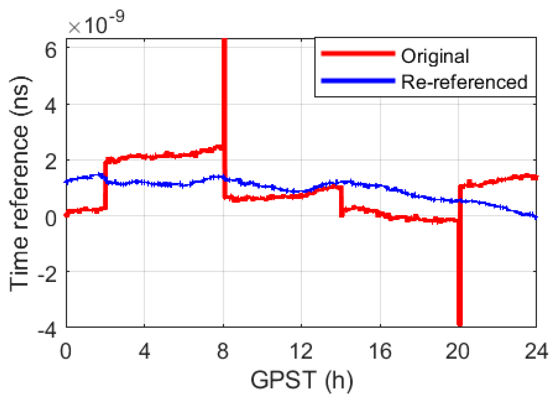
- Poor stability of the real-time LEO satellite clock time reference due to the poor stability of the time reference of the real-time GNSS satellite clocks, as shown in Figure 3 (red). In Figure 3, the real-time time reference is calculated as the epoch mean difference between all the usable real-time GPS satellite clocks from the CNES and the CODE final GPS satellite clocks [18].
2.2. LEO Satellite Clock Prediction in Ultra-Short-Term
2.3. LEO Satellite Clock Broadcasting for Real-Time Applications
3. Processing Strategies
- (1)
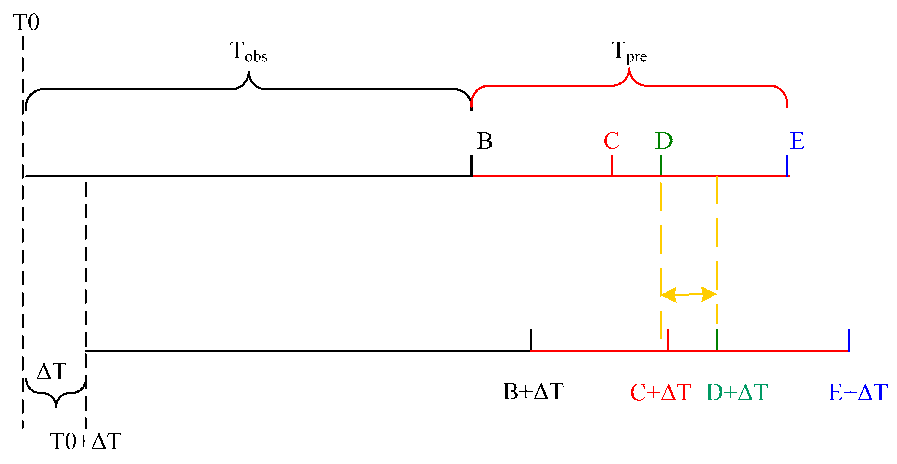
- At the current time point , acquire observational data in [], and obtain real-time GNSS products selected according to Section 2.1;
- (2)
- Based on the strategies outlined in Table 2, determine the LEO satellite clocks in near-real-time;
- (3)
- According to the prediction method detailed in Section 2.2, predict the LEO satellite clocks over .
- (4)
- Perform a second-order polynomial fitting using the predicted clocks, and broadcast the fitted polynomial coefficients to users;
4. Test Results
4.1. Near-Real-Time LEO Satellite Clocks
4.2. Real-Time LEO Satellite Clocks
- (1)
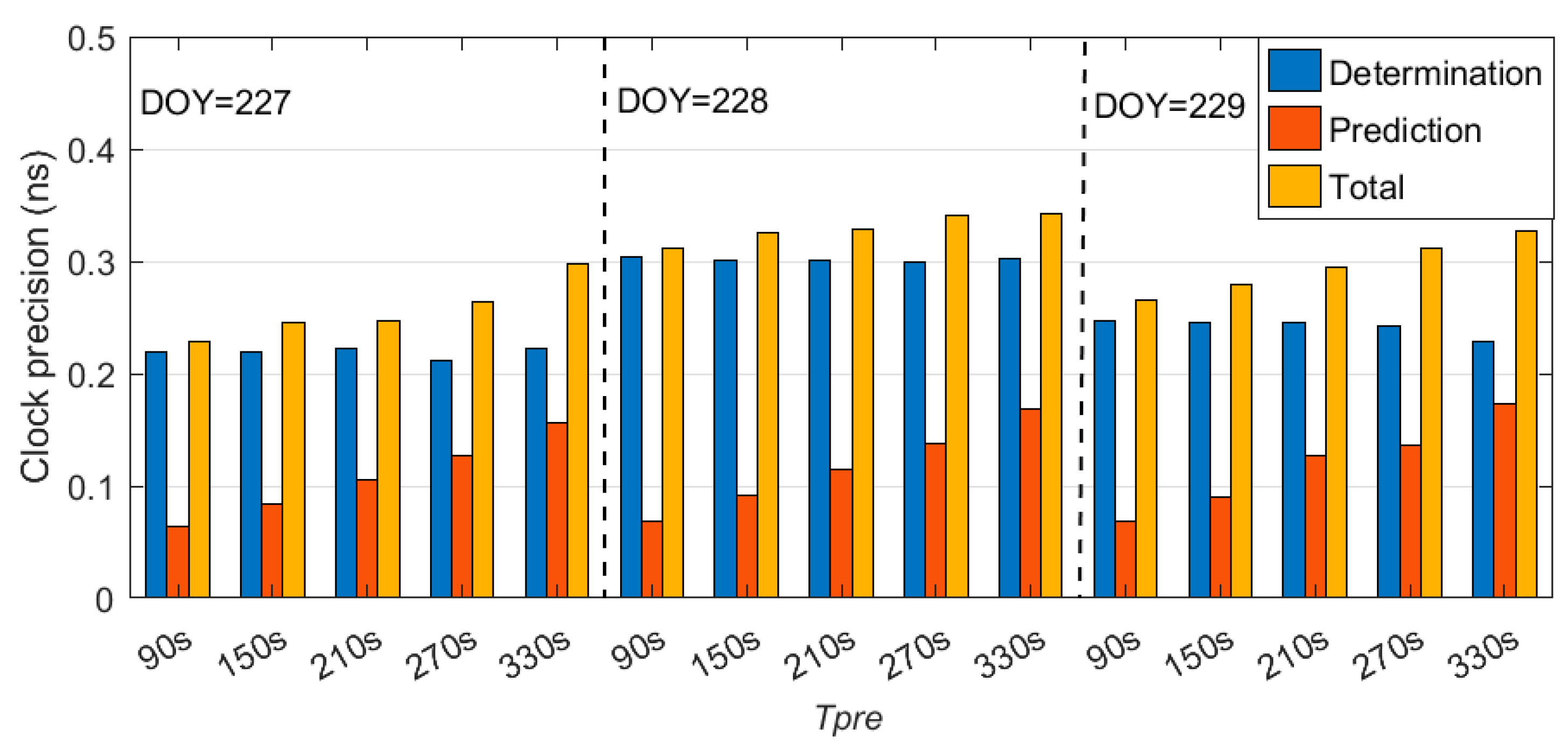
- The processing time is mainly dependent on the processing arc length . For the very similar , it is preferable to have a longer to enhance the short-term stability of the near-real-time clocks. The time interval between subsequent processing sessions () is independent of the precision of the near-real-time clocks but directly determines the prediction time and the usable prediction window [, ] for real-time applications. The latter is directly related to the predicted clock precision, i.e., the precision of real-time LEO satellite clocks.
- (2)
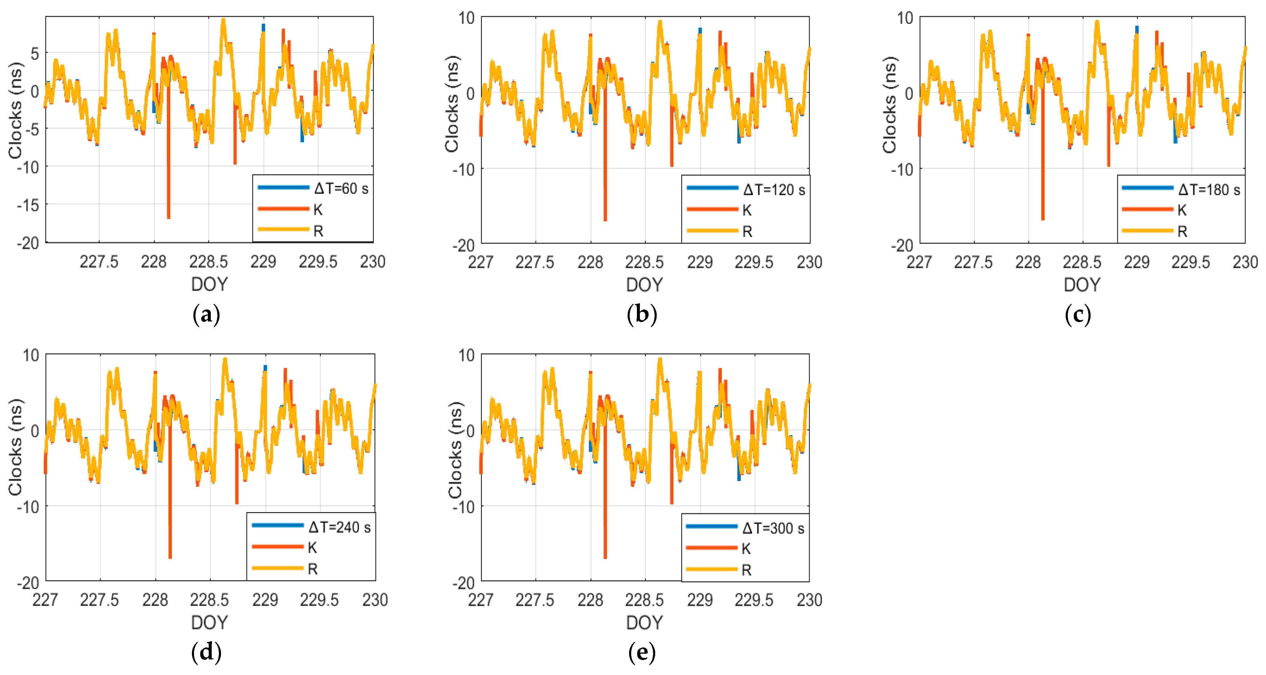
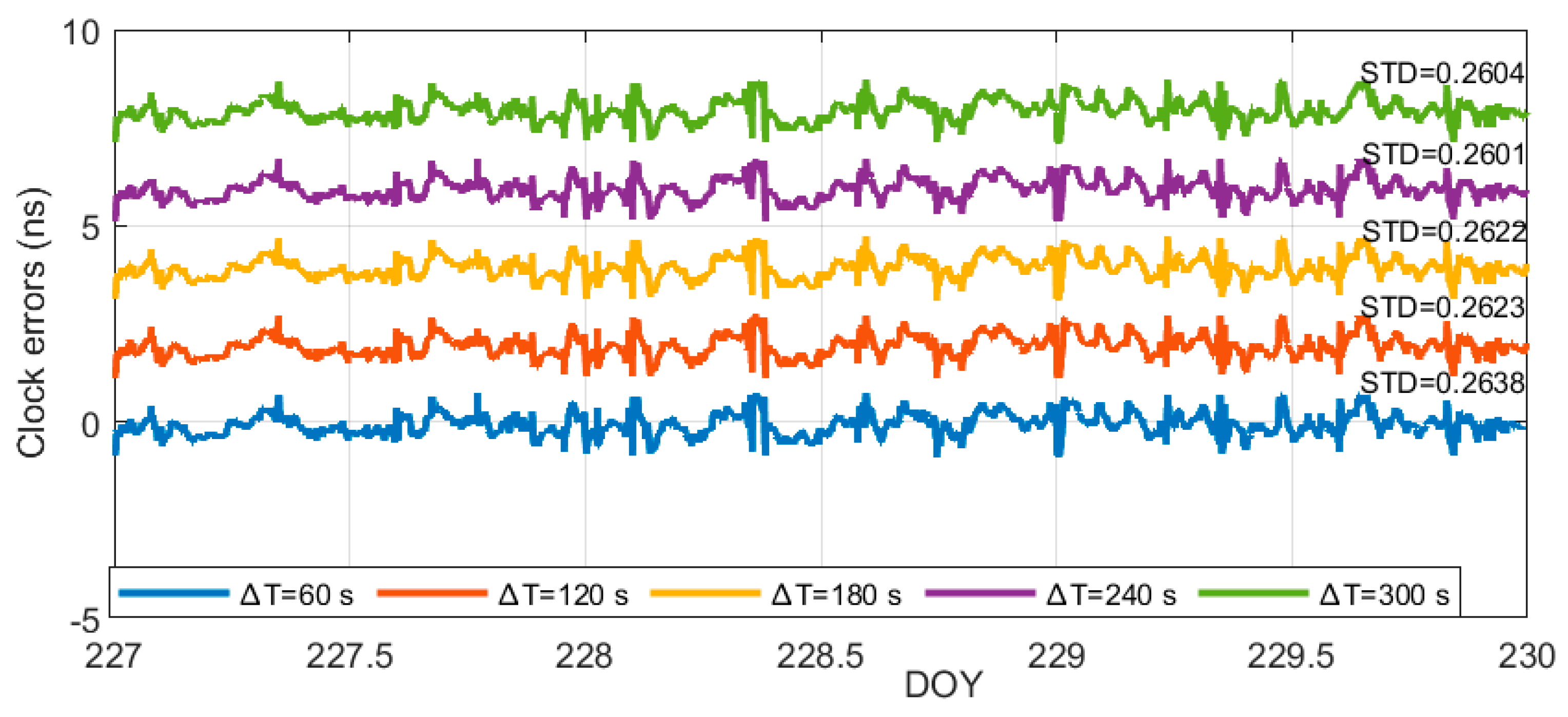
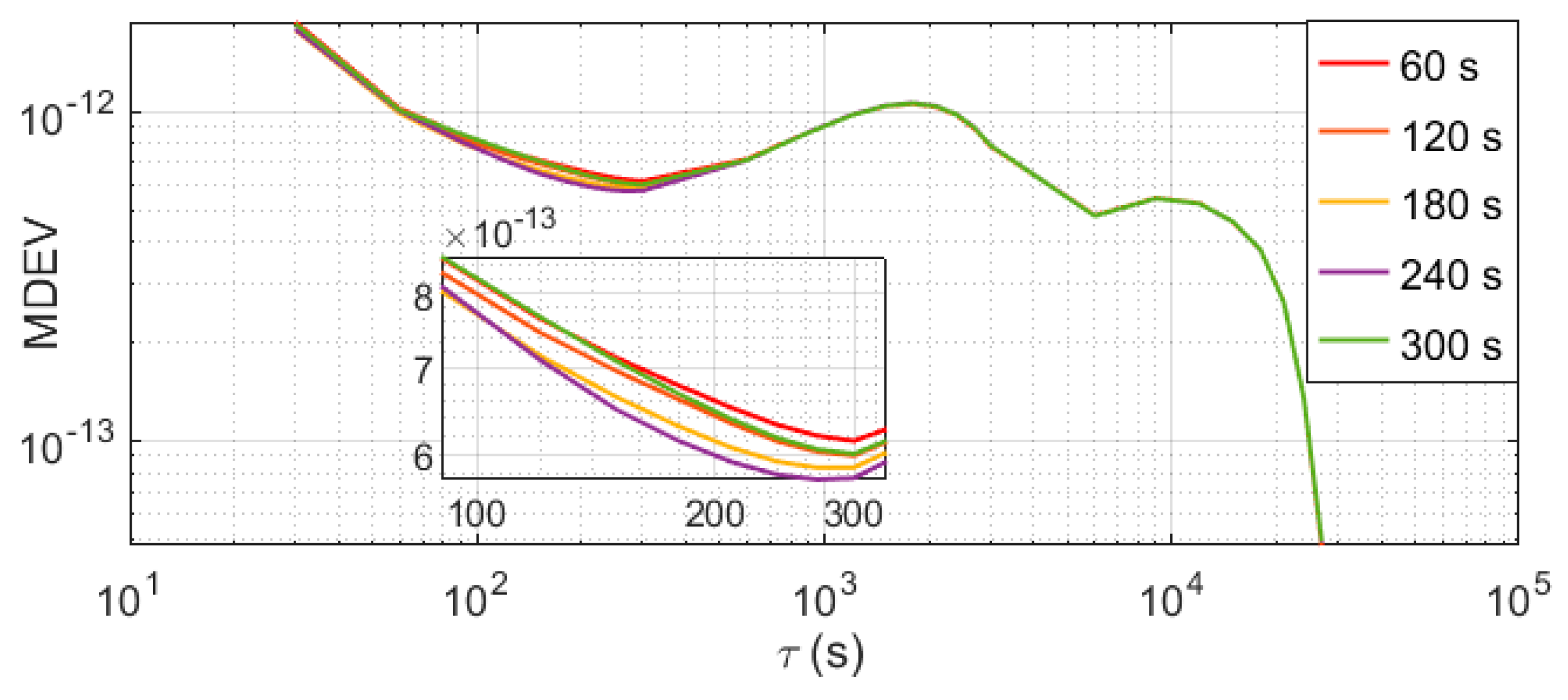
- The precision of the connected near-real-time LEO satellite clocks of the last period within the 6 h processing arcs is similar to the kinematic daily solutions. The major differences in the real-time clocks for different come from the clock prediction, more concretely, from the different prediction times. Further research is needed to improve the ultra-short-term prediction of LEO satellite clocks, i.e., within 5 min.
- (3)
- When setting to 60 s, a real-time clock precision around or lower than 0.3 ns can be achieved.
5. Discussion and Conclusions
Author Contributions
Funding
Data Availability Statement
Conflicts of Interest
References
- Wang, L.; Li, D.; Chen, R.; Fu, W.; Shen, X.; Jiang, H.; Hao, J. Low earth orbiter (LEO) navigation augmentation: Opportunities and challenges. Strateg. Study CAE 2020, 22, 144–152. [Google Scholar]
- Starlink. Available online: https://www.starlink.com/ (accessed on 26 February 2024).
- Eutelsat OneWeb. Available online: https://oneweb.net/ (accessed on 26 February 2024).
- Iridium Satellite Communications. Available online: https://www.iridium.com/ (accessed on 26 February 2024).
- Xona Space Systems. Available online: https://www.xonaspace.com/ (accessed on 26 February 2024).
- Kepler. Available online: https://www.kepler.global/conf/system/ (accessed on 26 February 2024).
- Li, W.; Yang, Q.; Du, X.; Li, M.; Zhao, Q.; Yang, L.; Qin, Y.; Chang, C.; Wang, Y.; Qin, G. LEO augmented precise point positioning using real observations from two CENTISPACE™ experimental satellites. GPS Solut. 2024, 28, 44. [Google Scholar] [CrossRef]
- Zhang, X.; Ma, F. Review of the development of LEO navigation-augmented GNSS. Acta Geod. Cartogr. Sin. 2019, 48, 1073. [Google Scholar]
- Yi, H.; Lei, W.; Wenju, F.; Haitao, Z.; Tao, L.; Beizhen, X.; Ruizhi, C. LEO navigation augmentation constellation design with the multi-objective optimization approaches. Chin. J. Aeronaut. 2021, 34, 265–278. [Google Scholar]
- Hauschild, A.; Tegedor, J.; Montenbruck, O.; Visser, H.; Markgraf, M. Precise onboard orbit determination for LEO satellites with real-time orbit and clock corrections. In Proceedings of the 29th International Technical Meeting of the Satellite Division of The Institute of Navigation (ION GNSS+ 2016), Portland, OR, USA, 12–16 September 2016; pp. 3715–3723. [Google Scholar]
- Li, K.; Zhou, X.; Guo, N.; Zhao, G.; Xu, K.; Lei, W. Comparison of precise orbit determination methods of zero-difference kinematic, dynamic and reduced-dynamic of GRACE-A satellite using SHORDE software. J. Appl. Geod. 2017, 11, 157–165. [Google Scholar] [CrossRef]
- Wang, K.; Liu, J.; Su, H.; El-Mowafy, A.; Yang, X. Real-time LEO satellite orbits based on batch least-squares orbit determination with short-term orbit prediction. Remote Sens. 2022, 15, 133. [Google Scholar] [CrossRef]
- Hauschild, A.; Montenbruck, O.; Steigenberger, P.; Martini, I.; Fernandez-Hernandez, I. Orbit determination of Sentinel-6A using the Galileo high accuracy service test signal. GPS Solut. 2022, 26, 120. [Google Scholar] [CrossRef]
- Wang, K.; Yang, X.; El-Mowafy, A. Visibility of LEO Satellites under Different Ground Network Distributions. In Proceedings of the 35th International Technical Meeting of the Satellite Division of The Institute of Navigation (ION GNSS+ 2022), Denver, CO, USA, 19–23 September 2022; pp. 2478–2491. [Google Scholar]
- Montenbruck, O.; Ramos-Bosch, P. Precision real-time navigation of LEO satellites using global positioning system measurements. GPS Solut. 2008, 12, 187–198. [Google Scholar] [CrossRef]
- El-Mowafy, A.; Wang, K.; Li, Y.; Allahvirdi-Zadeh, A. The impact of orbital and clock errors on positioning from LEO constellations and proposed orbital solutions. Int. Arch. Photogramm. Remote Sens. Spat. Inf. Sci. 2023, 48, 1111–1117. [Google Scholar] [CrossRef]
- Montenbruck, O.; Hackel, S.; Wermuth, M.; Zangerl, F. Sentinel-6A precise orbit determination using a combined GPS/Galileo receiver. J. Geod. 2021, 95, 109. [Google Scholar] [CrossRef]
- Wang, K.; El-Mowafy, A. LEO satellite clock analysis and prediction for positioning applications. Geo Spat. Inf. Sci. 2022, 25, 14–33. [Google Scholar] [CrossRef]
- Wu, M.; Wang, K.; Liu, J.; Zhu, Y. Relativistic effects of LEO satellite and its impact on clock prediction. Meas. Sci. Technol. 2023, 34, 095005. [Google Scholar] [CrossRef]
- Ge, H.; Wu, T.; Li, B. Characteristics analysis and prediction of Low Earth Orbit (LEO) satellite clock corrections by using least-squares harmonic estimation. GPS Solut. 2023, 27, 38. [Google Scholar] [CrossRef]
- Suesser-Rechberger, B.; Krauss, S.; Strasser, S.; Mayer-Guerr, T. Improved precise kinematic LEO orbits based on the raw observation approach. Adv. Space Res. 2022, 69, 10. [Google Scholar] [CrossRef]
- Yang, Z.; Liu, H.; Qian, C.; Shu, B.; Zhang, L.; Xu, X.; Zhang, Y.; Lou, Y. Real-time estimation of low Earth orbit (LEO) satellite clock based on ground tracking stations. Remote Sens. 2020, 12, 2050. [Google Scholar] [CrossRef]
- Yang, Z.; Liu, H.; Wang, P.; Xu, X.; Qian, C.; Shu, B.; Zhang, Y. Integrated kinematic precise orbit determination and clock estimation for low Earth orbit satellites with onboard and regional ground observations. Meas. Sci. Technol. 2022, 33, 125002. [Google Scholar] [CrossRef]
- Yang, Y. PPP Based Sequential Orbit Determination for Satellite in Low Earth Orbit. Ph.D. Thesis, Northwestern Polytechnical University, Xi’An, China, 2015. [Google Scholar]
- IGS Real-Time Service. Available online: https://igs.org/rts/ (accessed on 26 February 2024).
- International GNSS Monitoring & Assessment System. Available online: http://www.igmas.org/Product/Info/ (accessed on 26 February 2024).
- Bock, H.; Dach, R.; Jäggi, A.; Beutler, G. High-rate GPS clock corrections from CODE: Support of 1 Hz applications. J. Geod. 2009, 83, 1083–1094. [Google Scholar] [CrossRef]
- Rülke, A.; Agrotis, L.; Caissy, M.; Habrich, H.; Neumaier, P.; Söhne, W.; Weber, G. IGS Real-Time Service-Status And Future Developments. In Proceedings of the EGU General Assembly Conference, Vienna, Austria, 27 April–2 May 2014; p. 7429. [Google Scholar]
- Hadas, T.; Bosy, J. IGS RTS precise orbits and clocks verification and quality degradation over time. GPS Solut. 2015, 19, 93–105. [Google Scholar] [CrossRef]
- Kazmierski, K.; Sośnica, K.; Hadas, T. Quality assessment of multi-GNSS orbits and clocks for real-time precise point positioning. GPS Solut. 2018, 22, 11. [Google Scholar] [CrossRef]
- BKG—Bundesamt für Kartographie und Geodäsie. Available online: https://www.bkg.bund.de/ (accessed on 26 February 2024).
- Tobías, G.; Calle, J.D.; Navarro, P.; Rodríguez, I.; Rodríguez, D. magicGNSS’ Real-Time POD and PPP Multi-GNSS Service. In Proceedings of the 27th International Technical Meeting of the Satellite Division of The Institute of Navigation (ION GNSS+ 2014), Tampa, FL, USA, 8–12 September 2014. [Google Scholar]
- Guo, L.; Zhao, Q.; Xu, X.; Tao, J.; Zhang, Q.; Qu, Z.; Chen, G.; Wang, C. Real-time orbit and clock products at Wuhan University to support Multi-GNSS applications. In Proceedings of the IGS Workshop, Wuhan, China, 29 October–2 November 2018. [Google Scholar]
- Männel, B.; Brandt, A.; Nischan, T.; Brack, A.; Sakic, P.; Bradke, M. GFZ Rapid Product Series for the IGS; GFZ Data Services; GFZ: Potsdam, Germany, 2020. [Google Scholar]
- Chen, B.; Wang, K.; El-Mowafy, A.; Yang, X. Real-Time GNSS satellite SISRE and its integrity for LEO satellite Precise Orbit Determination. In Proceedings of the 2024 International Technical Meeting of The Institute of Navigation (ION ITM 2024), Long Beach, CA, USA, 22–25 January 2024. [Google Scholar]
- Prange, L.; Orliac, E.; Dach, R.; Arnold, D.; Beutler, G.; Schaer, S.; Jäggi, A. CODE’s five-system orbit and clock solution—The challenges of multi-GNSS data analysis. J. Geod. 2017, 91, 345–360. [Google Scholar] [CrossRef]
- Larson, K.M.; Ashby, N.; Hackman, C.; Bertiger, W. An assessment of relativistic effects for low Earth orbiters: The GRACE satellites. Metrologia 2007, 44, 484. [Google Scholar] [CrossRef]
- Ko, U.-D.; Tapley, B.D. Computing the USO frequency instability of GRACE satellites. In Proceedings of the 2010 IEEE Aerospace Conference, Big Sky, MT, USA, 6–13 March 2010; pp. 1–8. [Google Scholar]
- Hudson, A.I.; Iyanu, G.H.; Wang, H.; Bloch, M.B.; McClelland, T.; Terracciano, L. Long-term Performance of a Space-system OCXO. In Proceedings of the 2019 Joint Conference of the IEEE International Frequency Control Symposium and European Frequency and Time Forum (EFTF/IFC), Orlando, FL, USA, 14–18 April 2019; IEEE: Piscataway, NJ, USA, 2019. [Google Scholar]
- Fletcher, K. Sentinel-3: ESA’s Global Land and Ocean Mission for GMES Operational Services; ESA Communications: Oakville, ON, Canada, 2012. [Google Scholar]
- Riley, W. Handbook of Frequency Stability Analysis; NIST special publication 1065; NIST: Gaithersburg, MD, USA, 2008.


| (h) | (s) | STD (vs. K) (ns) | STD (vs. R) (ns) |
|---|---|---|---|
| 24 | 24 | --- | --- |
| 12 | 21 | 0.015 | 0.19 |
| 8 | 19 | 0.015 | 0.19 |
| 6 | 18 | 0.015 | 0.20 |
| 4 | 17 | 0.018 | 0.20 |
| 2 | 17 | 0.048 | 0.22 |
| Type | Parameters | Processing Strategies |
|---|---|---|
| Near-real-time clock determination | Observations | Undifferenced IF code and carrier phase combination (GPS: L1/L2) |
| Sampling | 30 s | |
| Elevation cut-off angle | 3° | |
| GNSS orbits and clocks | Selected (Section 2.1) | |
| GNSS satellite antenna PCO/PCVs | igs20.atx | |
| LEO satellite antenna PCO/PCVs | Operator supplied | |
| Phase wind-up | Corrected | |
| Estimatior | Kalman filter, Kinematic | |
| 6 h | ||
| Clock Prediction | Longer than | |
| 60/120/180/240/300 s | ||
| Broadcast interval | Optional |
| DOY | STD (K vs. R) (ns) | (s) | STD (vs. K) (ns) | STD (vs. R) (ns) |
|---|---|---|---|---|
| 227 | 0.211 | 60 | 0.025 | 0.218 |
| 120 | 0.021 | 0.218 | ||
| 180 | 0.018 | 0.218 | ||
| 240 | 0.015 | 0.215 | ||
| 300 | 0.015 | 0.201 | ||
| 228 | 0.297 | 60 | 0.025 | 0.304 |
| 120 | 0.021 | 0.300 | ||
| 180 | 0.018 | 0.300 | ||
| 240 | 0.014 | 0.299 | ||
| 300 | 0.025 | 0.301 | ||
| 229 | 0.237 | 60 | 0.028 | 0.246 |
| 120 | 0.024 | 0.245 | ||
| 180 | 0.020 | 0.245 | ||
| 240 | 0.017 | 0.241 | ||
| 300 | 0.028 | 0.230 |
| DOY | (s) | (s) | Fitting Time (s) | STD of Near-Real-Time Clocks Used for Fitting (ns) | Precision Loss (ns) | STD (vs. R) (ns) |
|---|---|---|---|---|---|---|
| 227 | 60 | 90 | 120 | 0.219 | 0.064 | 0.229 |
| 120 | 150 | 180 | 0.219 | 0.084 | 0.246 | |
| 180 | 210 | 180 | 0.222 | 0.106 | 0.247 | |
| 240 | 270 | 270 | 0.211 | 0.127 | 0.264 | |
| 300 | 330 | 300 | 0.223 | 0.156 | 0.297 | |
| 228 | 60 | 90 | 120 | 0.304 | 0.069 | 0.311 |
| 120 | 150 | 180 | 0.301 | 0.092 | 0.326 | |
| 180 | 210 | 180 | 0.301 | 0.115 | 0.329 | |
| 240 | 270 | 270 | 0.299 | 0.138 | 0.341 | |
| 300 | 330 | 300 | 0.303 | 0.169 | 0.342 | |
| 229 | 60 | 90 | 120 | 0.247 | 0.068 | 0.266 |
| 120 | 150 | 180 | 0.245 | 0.090 | 0.279 | |
| 180 | 210 | 180 | 0.246 | 0.127 | 0.295 | |
| 240 | 270 | 270 | 0.243 | 0.136 | 0.312 | |
| 300 | 330 | 300 | 0.228 | 0.173 | 0.327 |
Disclaimer/Publisher’s Note: The statements, opinions and data contained in all publications are solely those of the individual author(s) and contributor(s) and not of MDPI and/or the editor(s). MDPI and/or the editor(s) disclaim responsibility for any injury to people or property resulting from any ideas, methods, instructions or products referred to in the content. |
© 2024 by the authors. Licensee MDPI, Basel, Switzerland. This article is an open access article distributed under the terms and conditions of the Creative Commons Attribution (CC BY) license (https://creativecommons.org/licenses/by/4.0/).
Share and Cite
Wu, M.; Wang, K.; Wang, J.; Liu, J.; Chen, B.; Xie, W.; Zhang, Z.; Yang, X. Real-Time LEO Satellite Clocks Based on Near-Real-Time Clock Determination with Ultra-Short-Term Prediction. Remote Sens. 2024, 16, 1326. https://doi.org/10.3390/rs16081326
Wu M, Wang K, Wang J, Liu J, Chen B, Xie W, Zhang Z, Yang X. Real-Time LEO Satellite Clocks Based on Near-Real-Time Clock Determination with Ultra-Short-Term Prediction. Remote Sensing. 2024; 16(8):1326. https://doi.org/10.3390/rs16081326
Chicago/Turabian StyleWu, Meifang, Kan Wang, Jinqian Wang, Jiawei Liu, Beixi Chen, Wei Xie, Zhe Zhang, and Xuhai Yang. 2024. "Real-Time LEO Satellite Clocks Based on Near-Real-Time Clock Determination with Ultra-Short-Term Prediction" Remote Sensing 16, no. 8: 1326. https://doi.org/10.3390/rs16081326
APA StyleWu, M., Wang, K., Wang, J., Liu, J., Chen, B., Xie, W., Zhang, Z., & Yang, X. (2024). Real-Time LEO Satellite Clocks Based on Near-Real-Time Clock Determination with Ultra-Short-Term Prediction. Remote Sensing, 16(8), 1326. https://doi.org/10.3390/rs16081326