

Practical Limitations of Using the Tilt Compensation Function of the GNSS/IMU Receiver

1
Faculty of Civil Engineering Subotica, University of Novi Sad, 24000 Subotica, Serbia
2
Department School of Civil Engineering and Geodesy of Applied Studies, Academy of Technical and Art Applied Studies Belgrade, 11000 Belgrade, Serbia
*
Author to whom correspondence should be addressed.
Remote Sens. 2024, 16(8), 1327; https://doi.org/10.3390/rs16081327
Submission received: 25 February 2024
/
Revised: 31 March 2024
/
Accepted: 4 April 2024
/
Published: 10 April 2024
(This article belongs to the Special Issue BDS/GNSS for Earth Observation: Part II)
Abstract
:The research in this paper is related to the accuracy of the tilt compensation function of the GNSS/IMU receivers, which were examined in an open sky environment. The purpose of the paper is to point out to geodesists the conditions and limitations of using GNSS/IMU technology in precise measurements to not jeopardize the coordinate’s accuracy. The environment in which the measurement is made affects the quality of the GNSS signal and can limit the visibility of the satellite, leading to larger errors in the measurement. In this experiment, the current performance of the GNSS/IMU receivers was checked. Seven GNSS/IMU receivers were used for the realization of the experiment. For six receivers the compensation angle was α = 30°, while for one receiver, the compensation angle was α = 45°. The standard uncertainty of GNSS coordinates of the antenna phase center has values less than 9 mm. The standard uncertainty of the IMU component has values less than 31 mm. The measurement uncertainty of the position of the used GNSS receivers is in the range of 18.1 mm to 31.7 mm. The limit values for the differences along the coordinate axes x and y were determined, and their values are from 26 mm to 44 mm. In the conducted experiment, it was confirmed that three GNSS/IMU receivers have a “Satisfactory” result. The results show that GNSS/IMU measurements with a slope greater than 30° significantly affect the accuracy and reliability of GNSS/IMU technology. A slope greater than 45° has a deviation along the coordinate axes of 121.3 mm. The conducted research is particularly important for geodetic works that require high positioning performance. The testing method of the GNSS/IMU receiver presented in this paper can help its users to make correct conclusions regarding the coordinate accuracy of the measured point of interest.

1. Introduction
In real-time kinematic positioning (RTK) using the GNSS (global navigation satellite system), it is of the utmost importance to determine the coordinates of the point of interest (POI) with a high degree of accuracy. It is important for geodetic networks, for monitoring objects under construction during their exploitation period, for landslide monitoring, etc. The accuracy of the coordinates is directly related to the errors of the measured values. The errors that follow each measurement are divided into random and systematic.
In GNSS RTK positioning, the pole on which the receiver antenna is mounted should be positioned vertically. A GNSS RTK receiver does not measure the coordinates directly at the point of interest but at the phase center of the antenna, so the position of the antenna phase center (APC) is lowered to the point of interest on the ground, using the value of the vertical displacement (receiver pole height) between the APC and point of interest [1]. Unfortunately, it is not always possible to hold the receiver pole in a vertical position due to human errors, the inaccessibility of the POI (for example: when measuring the corners of a building, when measuring under a canopy, etc.), when the surveyor’s safety is threatened on traffic roads or the edges of deep ravines and pits. Therefore, a GNSS receiver with a tilt compensation function is considered a real advancement in measurement efficiency and reliability.
More than two decades have passed since the first tilt compensation functions were integrated into GNSS rovers. The first tilt compensation was performed using magnetic compass orientation [2], which often required complex calibration procedures. Magnetic compass measurements are affected by magnetic disturbances caused by cars, steel structures and electrical installations that are usually present in environments where measurements are made with a GNSS RTK receiver. The magnetic field measured on the magnetometer varies significantly with the tilt angle, limiting the tilt compensation range up to 15 degrees [3]. Although such features represented gains in efficiency, they were partially accepted by end users and did not find widespread use.
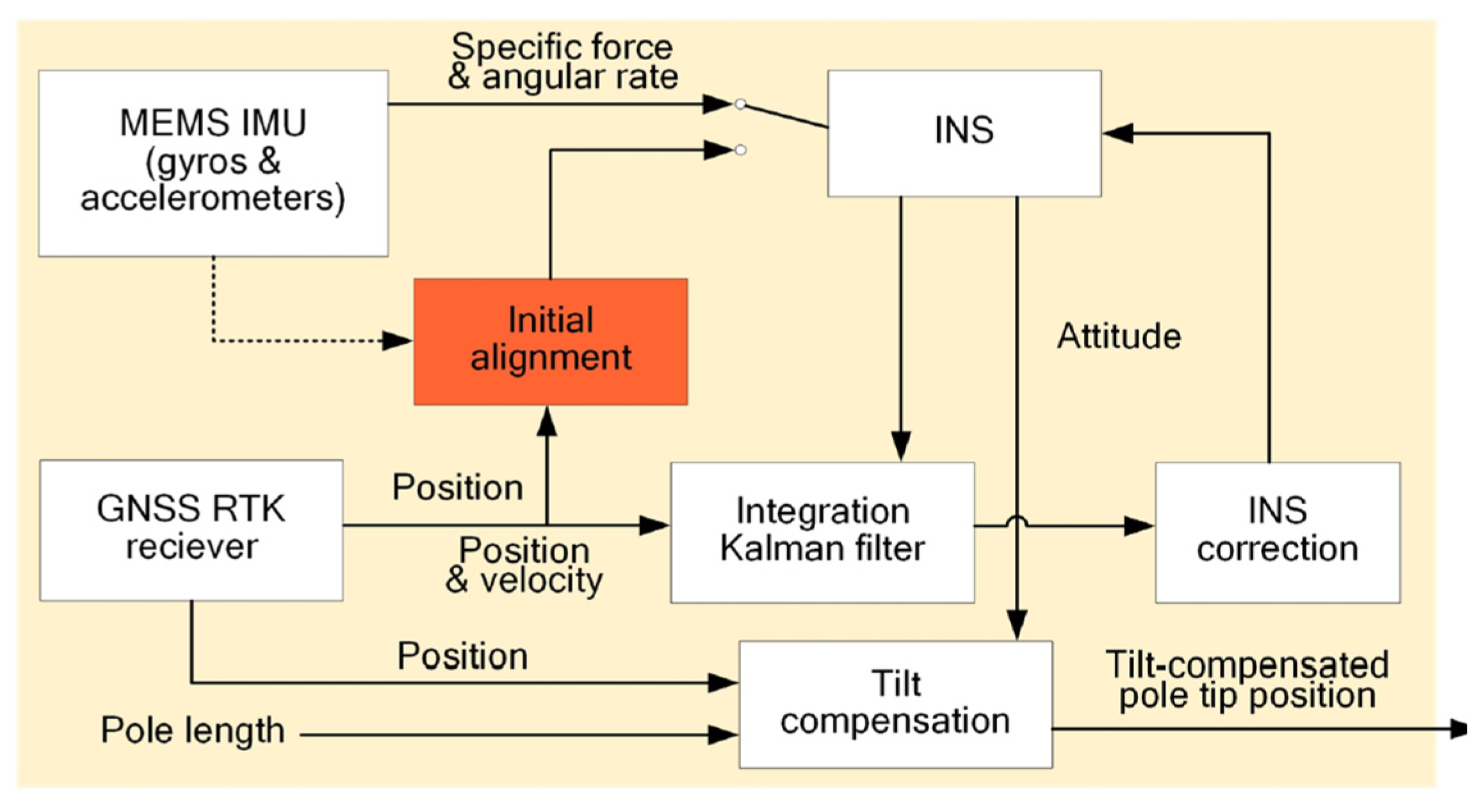
The next generation of GNSS receivers integrates an inertial measurement unit (IMU) for its orientation. The integration of GNSS and IMU technology, often called the GNSS inertial navigation system (INS), provides a precise solution for navigation and positioning in various applications [4]. The latest generations of GNSS RTK receivers are equipped with special sensors for measuring the tilt of the receiver, i.e., the deviation from its vertical position. The role of the sensor is to determine the tilt/incline and to eliminate the resulting error by introducing a correction. A GNSS RTK receiver with a tilt compensation function uses two navigation technologies: a three-axis accelerometer and a three-axis gyroscope in the micro-electro-mechanical sensor (MEMS) component of the IMU. Precise acceleration and angular velocity measurements from the IMU are provided to the INS, along with high-rate position and velocity estimates from the GNSS. “Determining the pole holding based on a built-in inertial navigation system aided by RTK positions has become the mainstream in the latest generation of tilted GNSS RTK receivers”. Figure 1 depicts the data processing scheme of an IMU-based tilted GNSS RTK receiver. The position of the IMU center from the Kalman filter is used in tilt compensation to obtain the position of the pole tip [5]. The Kalman filter is used to integrate information obtained from the GNSS (high-frequency position and velocity estimates) and IMU (acceleration and angular rotation measurements). Kalman filters enable adaptive filtering and data integration, while INS corrections contribute to correcting errors in the inertial navigation system. By combining these two techniques, GNSS RTK receivers with tilt compensation functions achieve high accuracy and reliability in determining position and orientation in various conditions. Based on the GNSS RTK position, INS position and receiver pole length, the software itself calculates the tilt-compensated pole position at the POI.
In practice, the surveyor uses this equipment to perform measurements at inaccessible ground points. The newest tilt compensation technology makes geodetic measurements much more practical and extends the application of GNSS RTK in restrictive environments (such as covered places, dense jungles, buildings, hiding points and dangerous points) [6,7,8].
To buy a GNSS RTK receiver with a built-in tilt compensation function, the purchaser has to pay extra to the manufacturer. Due to the high added costs, owners of the private geodetic organization in the Republic of Serbia (RS) often give up on this option. However, in the market of the Republic of Serbia, some manufacturers of GNSS RTK receivers, in order to be more competitive, decided to offer the tilt compensation function for a significantly lower price that is acceptable for the geodetic organization. User experiences with those GNSS/IMU receiver manufacturers vary depending on the specifics of the GNSS receiver model, work environment and the type of work being performed by the geodetic organization. Therefore, everyone agrees that the technology is insufficiently tested and, whenever possible, they measure with the GNSS RTK receiver placed vertically with the receiver pole, i.e., without the tilt compensation function turned on. Users of GNSS/IMU receivers in the Republic of Serbia have confirmed that tilt compensation technology offers a great advantage in restrictive environments but share the common opinion that there is little information about the quality of POI coordinates. Private investment in permanent GNSS network stations in the RS has led to an increased use of GNSS receivers in various sectors, including precision measurement and navigation. Existing studies often focus on general GNSS characteristics and the modeling of atmospheric effects. The purpose of the research in this paper is to check and confirm the accuracy limits of the GNSS/IMU receiver through the analysis of the horizontal and vertical orientation of the instrument with the tilt compensation function. The value of this research is based on the use of different GNSS/IMU receivers that use different data processing software and that provide different tilt and accuracy levels. The positioning performance of the tilt compensation function of the GNSS/IMU receiver was checked in the experiment.
This paper is organized as an introduction to the known positioning performance of the GNSS receivers for static and kinematic positioning, presented in Section 2. In addition to positioning performance, it is important to check and investigate how GNSS/IMU technology works and how reliably this technology is, as presented in Section 3. Section 4 contains the results of checking the GNSS/IMU technology. A discussion of the obtained results is presented in Section 5, followed by a conclusion in Section 6.
2. Positioning Performance
Positioning performance generally refers to the accuracy, reliability and efficiency of determining the coordinates of the point of interest. It is a multidimensional concept that is influenced by various factors and includes the technology used, environmental conditions and specific user requirements. Positioning performance is the ultimate goal, but the steps taken to achieve high performance are calibration and checking. These three concepts are interrelated and are key to maintaining high standards in GNSS technology.
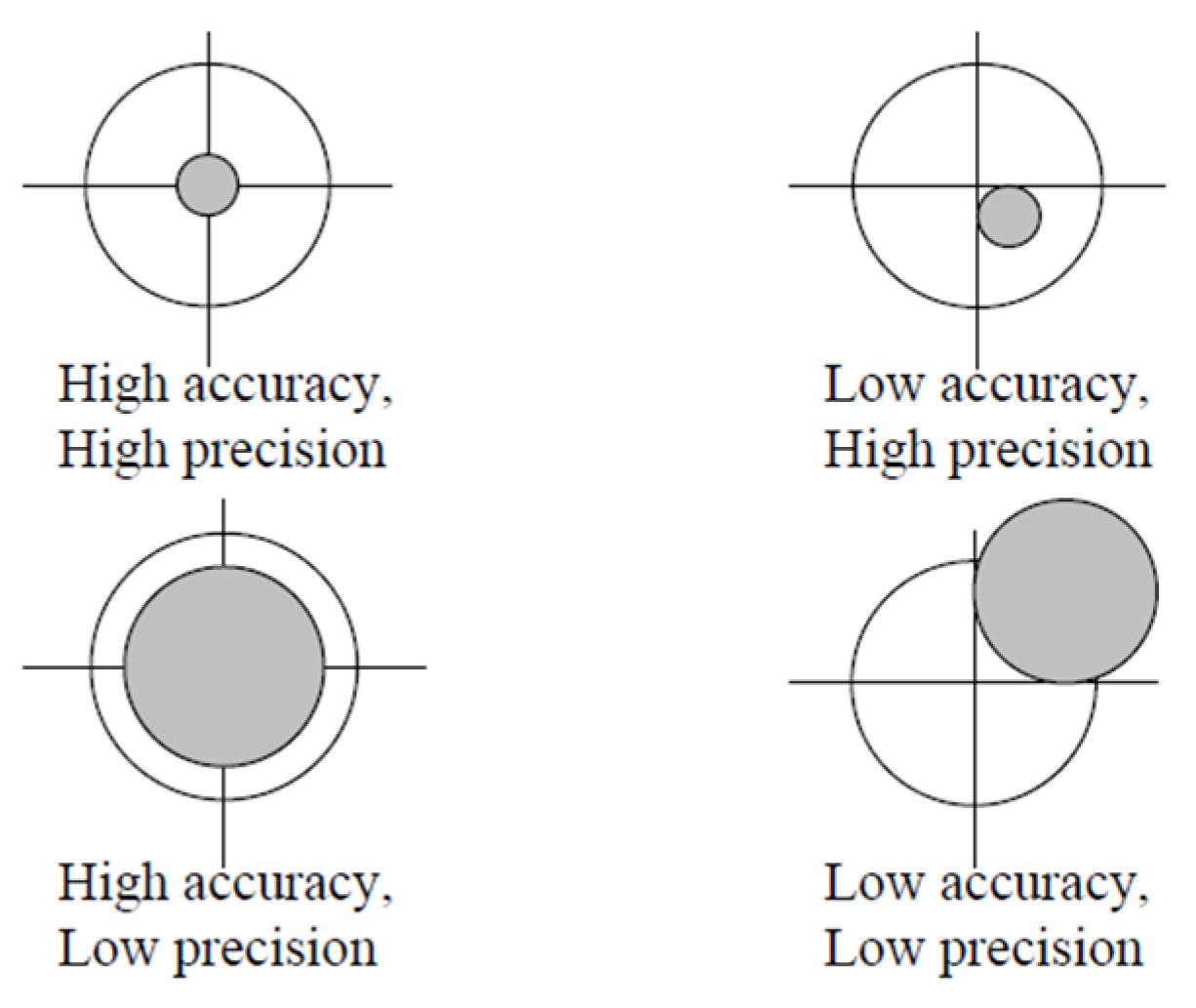
Geodesists use accuracy and precision as statistical methods to describe the quality of coordinates [9]. The difference between these two terms is presented in Figure 2.
The most commonly used measures of position accuracy (Table 1) are distance root mean squared (DRMS) and mean radial spherical error (MRSE). DRMS is a number that expresses 2D accuracy. MRSE is a measure of the accuracy of 3D coordinates extended by one dimension.
“High positioning performance” in GNSS positioning means that the GNSS receiver can reliably and accurately determine the position in different conditions and environments.
GNSS positioning is based on the data from multiple GNSS constellations: global positioning system (GPS—owned and operated by the United States of America), BeiDou (owned and operated by the People’s Republic of China), GALILEO (owned and operated by the European Union), GLObalnaya NAvigatsionnaya Sputnikovaya Sistema (GLONASS—owned and operated by the Russian Federation) and multiple available GNSS frequencies. It is a complex real-time process that aims to ensure centimeter-level positioning accuracy [10,11]. To evaluate the system-level performance, the following key parameters are used:
- Availability. The absolute number of RTK fixed solutions during a certain period.
- Accuracy. The deviation of RTK fixed positions from ground truth with a higher degree of accuracy, where the ground truth can be determined by using a total station or by post-processing long-term GNSS data.
- Reliability. The percentage that the position error (with respect to ground truth) is less than three times the corresponding estimate of the coordinate quality (CQ) [12].
Geodesist considers three types of accuracy:
- (a)
- Predicted accuracy—the accuracy of position determination by the system relative to the actual values;
- (b)
- Repeatable accuracy—the level of accuracy that allows the user to return to the coordinates determined earlier by the same system;
- (c)
- Relative accuracy—the ability to measure (determine) the coordinates relative to a different user within the same system at the same time [13].
Due to the wide application of GNSS technology, it is very important to analyze the methods of testing GNSS receivers and the accuracy achieved by their use. For geodetic surveying, the accuracy of the GNSS receiver is analyzed within static and kinematic positioning modes [14,15,16].
In this regard, UNAVCO (University NAVstar Consortium), a non-profit university-governed consortium that supports geoscience research and education using geodesy, must be mentioned. UNAVCO created the document: “Receiver and Antenna Test Report”, which aimed to help the academic research community to choose the appropriate GNSS receiver for its research [17]. UNAVCO tested several GNSS receivers and antennae in the field and compared the obtained GNSS results with ground truth. After that, all GNSS receivers were placed in an anechoic chamber, where the variations in the phase center of the APC were measured. The calibration method of the UNAVCO research community is considered a high-precision method for the calibration of GNSS receivers [18].
“However, for these procedures special calibration facilities and high expertise are necessary. Since the functionality of the individual components both hard and software is not known in detail anymore to the normal GPS user, for the geodetic practice only remains the system testing. In doing so, it should not be excluded from examining thereby individual influence parameters. Calibration and checking of measuring devices are traditional tasks of all metrological oriented engineers” [19].
The International Organization for Standardization (ISO) describes another method of calibration of GNSS RTK receivers, which is known as the field procedure and is described in the ISO 17123-8 standard [20], according to the model proposed by the National Geodetic Survey (NGS) [21]. The length of the GNSS baseline test field between two GNSS rover points should be from 2 m to 20 m [22].
In the process of GNSS RTK calibration, according to the procedure described in the ISO 17123-8 standard, the metrological characteristics of the GNSS RTK receiver should be confirmed. According to Clause 6: “Full test procedure” [20], the series of measurements consists of five measurements at rover points 1 and 2 (ground points of the test polygon). The RTK measurements should be carried out at intervals of five minutes. It takes about 30 min to perform one series of measurements, that is, to determine the horizontal (plane) coordinates (x and y) of ground points 1 and 2. The complete measurement procedure in “Full test procedure” consists of three series of measurements at intervals of five minutes, with the start time of successive series separated by at least 90 min.
It is necessary for each set of x and y coordinates (j = 1,..., 5) in the series (= 1, 2, 3) to calculate the horizontal distance between two rover points ( as follows:
Statistical testing involves calculating an arithmetic mean of the horizontal distance between two rover points () as follows:
Subsequently, calculated deviations from the nominal values () and standard deviations of a single horizontal distance can be calculated as follows:
where the following applies:
n is the total number of distance measurements that equal ;
is the nominal value of the horizontal distance.
A verification of metrological characteristics for horizontal and vertical positioning of GNSS RTK should be performed in an accredited laboratory.
Checking involves regularly monitoring the performance of the GNSS to determine whether the system is working properly and providing the expected positioning results. This process includes testing the accuracy of the coordinates in real conditions, comparing the results with reference values and analyzing the performance of the system in different weather conditions and environments.
3. Methods of Testing GNSS Receivers
“In addition to multi-frequency and multi-constellation GNSS positioning, dramatic advances in sensor fusion and computer vision in the last years continuously extend the applicability of cm level RTK through IMU-based tilt compensation and visual positioning technology” [12]. A measurement with IMU-based tilt compensation increases its area of use and efficiency only if the accuracy is satisfied.
The use of GNSS/IMU receivers with tilt compensation functions is a very attractive option for the geodetic profession. This option allows its users to reach an inaccessible POI, which would otherwise be impossible to measure with conventional GNSS receivers. The POIs that cannot be measured by conventional GNSS are known as “hidden” points to the surveyors. The accuracy defined by the GNSS manufacturer in the tilt compensation technology mode can be checked by various non-standard methods.
The accuracy of GNSS positioning is directly related to the geometric parameter and the atmosphere conditions. Geometric parameters refer to the number and position of GNSS satellites in the sky known as dilution of precision (DOP). Atmospheric conditions (ionospheric and tropospheric) are one of the biggest sources of errors in GNSS measurements [23]. Via the careful planning of GNSS measurements, errors arising from the atmospheric conditions and satellite geometry can be reduced [24]. The accuracy of the measured ground point coordinates depends on signal blockage conducted by the objects near the GNSS receiver, both natural and artificial.
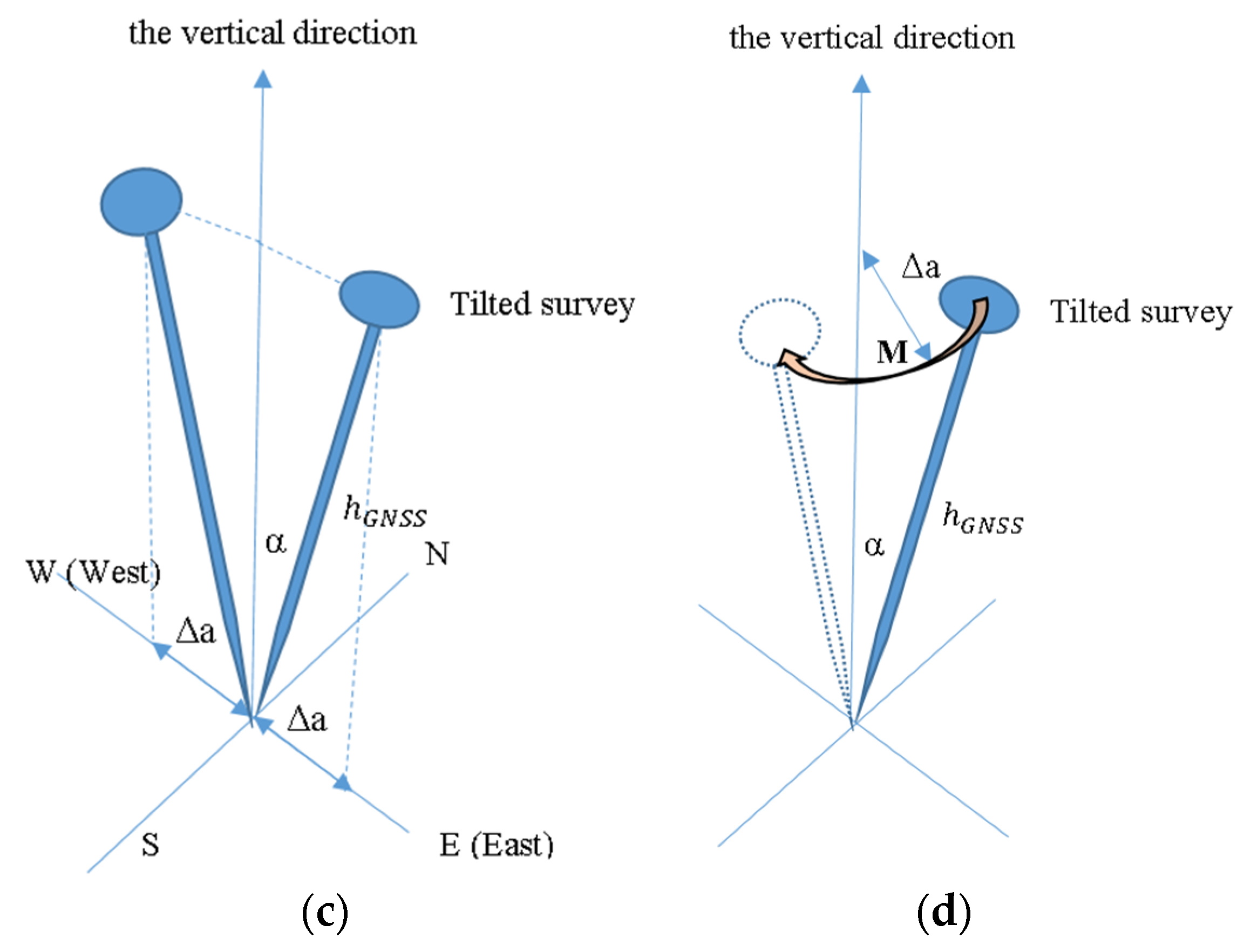
To minimize all these effects, the reference point of the test polygon for checking GNSS receivers with the tilt compensation function turned on should be placed in an open sky environment. The measurements should be performed with the same GNSS receiver pole height and controlled tilt value in four cardinal directions/positions: north, south, east and west (N, S, E, W) and while performing the conical motion (M) direction with the GNSS receiver, as presented in Figure 3. To achieve tilt control in all mentioned directions and for all tested GNSS/IMU receivers, the deviation from the antenna phase center to its vertical projection on the ground () could be calculated as follows:
where the following applies:
α is the tilt angle (defined as the angle between the vertical direction and the pole direction);
is the GNSS receiver pole height.
The experiment included three phases (Figure 3):
Phase 1. The GNSS/IMU checking process starts by placing the GNSS receiver pole in a vertical position at the test polygon reference point (Figure 3a). At the GNSS receiver vertical position, the center of the spirit level bubble placed on the GNSS receiver pole is in its center, and the tilt compensation function is turned off, i.e., the GNSS receiver pole is in “Position C” (Figure 3a). In that position, the first series of RTK measurements are performed.
Phase 2. Afterward, the tilt compensation function is turned on, and the GNSS receiver pole is tilted by the angle α toward all four cardinal directions: north, south, east and west (N, S, E, W), i.e., “Position N”, “Position S”, “Position E” and “Position W” (Figure 3b,c). Four consecutive series of RTK measurements at the same test polygon reference point are carried out.
Phase 3. The last coordinate measurements are performed while the GNSS receiver pole is in conical motion tilted by the angle α, i.e., “Position M” (Figure 3d).
3.1. Aspects of Data Processing
The coordinates of the GNSS/IMU receiver are expressed in the UTM coordinate system (B, L, h) and the coordinate system in the plane projection (x and y) [1]. To draw conclusions about the quality of the GNSS coordinates, basic statistics were calculated: the arithmetic mean, sample standard deviation and root mean square value for each coordinate in relation to the point that is defined as a reference point of the test polygon.
For the measured GNSS coordinates in each position of the GNSS receiver pole in Figure 3, the differences relative to the position of the GNSS receiver pole when the spirit level peaks, i.e., when the tilt compensation function is off and there are five consecutive positions of the GNSS receiver pole when the tilt compensation function is on, are calculated. The coordinate differences ( are calculated for the coordinates in the plane projection for the x and y direction as follows:
where the following applies:
are the measured coordinates when the GNSS receiver pole is in its vertical direction with the tilt compensation function turned off;
are the measured coordinates when the GNSS receiver pole is in four cardinal directions, and its motion direction with the tilt compensation function is turned on;
is the GNSS receiver position of measurements, with the tilt compensation function turned on toward the cardinal directions north, south, east and west (N, S, E, W) and while performing the conical motion (M) direction, as presented in Figure 3.
To test the significance of coordinate differences, it is necessary to calculate the sample standard deviation (, ) of each series as follows:
where the following applies:
are the arithmetic mean of coordinates from all series of measurement in each GNSS receiver pole position, respectively;
are a single measurement of the x and y coordinates;
is the number of measurements per each i position () of the GNSS receiver pole with the tilt compensation function turned on;
n is the total number of measurements that equal .
Based on the sample standard deviation, the experimental standard deviations () of a single x and y measurement can be calculated as follows:
where the sample standard deviations and are calculated via Equations (8) and (9), i.e., when the GNSS/IMU receiver tilt compensation function is turned off.
The total linear deviation of each measurement position (), when the tilt compensation function is turned on (), can be calculated as follows:
where is the GNSS receiver position of measurements with the tilt compensation function turned on toward the cardinal directions north, south, east and west (N, S, E, W) and while performing the conical motion (M) direction, as presented in Figure 3.
The positioning accuracy in RTK mode is defined by the standard deviation for horizontal and vertical positioning by the GNSS receiver manufacturer. The phase center of the GNSS antenna is located inside the receiver, while the point for which coordinates should be measured (ground point of interest) is located outside the GNSS receiver.
The coordinates of POIs are achieved by applying calculated phase center correction (PCC) to the coordinates of the phase center position. PCC is calculated using equations that are adjusted by manufacturers of GNSS receivers for every type of GNSS antenna they produce. GNSS/IMU receivers change this. “The Phase center correction (PCC) magnitude can reach the decimeter level according to the antenna structure. Therefore, the PCC model must be carefully handled in applications where phase observations are involved” [18]. For many years, GNSS/IMU-based solutions have been used for airborne, waterborne and mobile mapping systems, and now their application is being tested in geodetic class accuracy receivers for horizontal and vertical positioning. The research in this paper is related to the accuracy of the IMU tilt compensation function [3,25].
3.2. Accuracy Aspects of GNSS/IMU
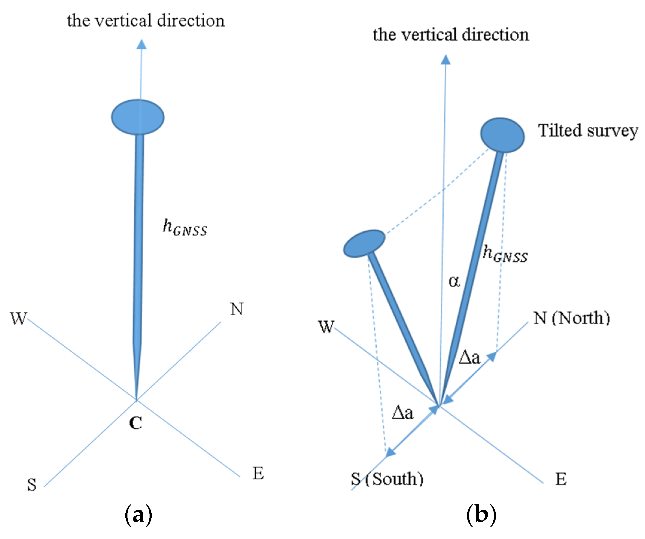
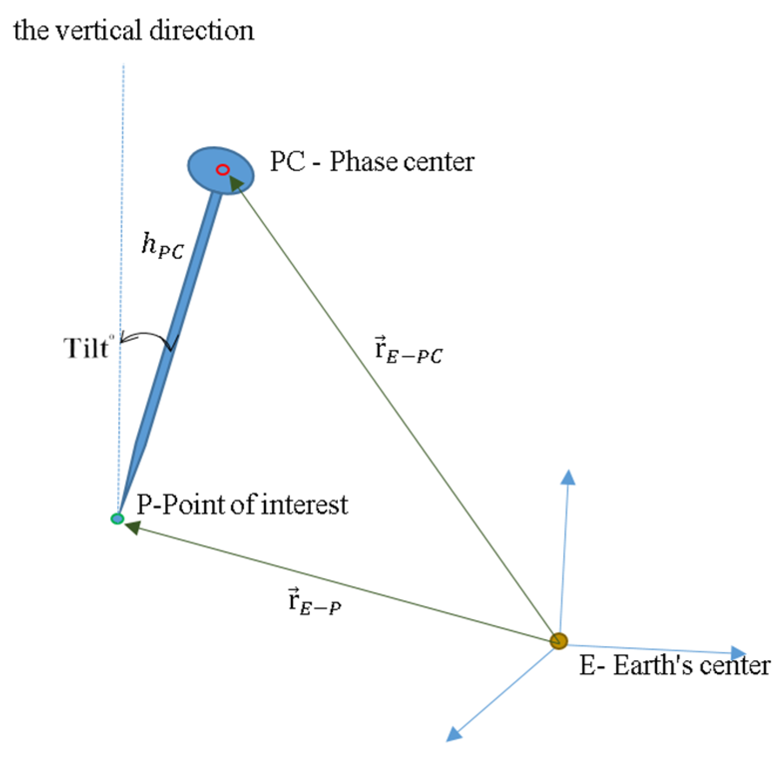
By direct measurement, the coordinates of the GNSS RTK receiver are always related to the phase center of the receiving GNSS antenna, i.e., to the point of the vector , shown in Figure 3. However, the point for which GNSS coordinates should be calculated is the point of interest (P) of the vector , shown in Figure 4. Acknowledging the fact that the GNSS receiver is placed on a pole whose height is known in advance and that it indicates the height of the phase center (, the position of point P is defined by a vector relation as follows:
“Assuming the pole is a rigid body, the error in the tilt-compensated pole tip position is mainly attributed to the GNSS position error and to the INS holding error” [6]. GNSS observation errors and GNSS/IMU component errors are uncorrelated in the measurement domain. The measurement uncertainty of the position of point P can be calculated as follows:
where the following applies:
denotes the pole tip position error;
is the standard uncertainty of GNSS coordinates of the APC (refers to the GNSS position error);
is the standard uncertainty of the INS component (refers to the position error induced by the IMU holding error).
The standard uncertainty of the GNSS coordinate of the APC as a contribution of certain sources of errors can be analyzed in accordance with the standard ISO 17123-8:2015 [20]. Typical influence quantities of the GNSS (RTK) must also be considered. Combined uncertainty () in the European Terrestrial Reference System 1989 (ETRS89) datum/Universal Transverse Mercator (UTM) projection horizontal coordinate system in zone 34N is described as follows:
while standard uncertainty on the vertical coordinate system is described as follows:
where the following applies:
is the standard uncertainty of xy coordinates;
is the standard uncertainty of h coordinates;
is the sensitivity of the tubular level on tribrach;
is the standard uncertainty of the minimum display digit;
is the standard uncertainty of the centering;
is the standard uncertainty of the antenna height;
is the stability of the bipod height, neglectable from the budget;
, and are standard uncertainties of the antenna phase center;
is the transformation;
is the standard uncertainty of the geoid undulation.
Therefore, the standard uncertainties of a single position () can be calculated as follows:
where the experimental standard deviations of a single measurement x and y are calculated by Equations (10) and (11).
It should be noted that the combined uncertainty on the horizontal coordinate system and the vertical coordinate system in the ISO 17123-8:2015 standard does not consider the following: the multipath; the clock in the GNSS receiver or satellite; the orbit of the satellite; ionospheric delay; tropospheric delay; and IMU tilt compensation.
The standard uncertainty of the IMU component (), which refers to the position error made by using tilt compensation technology, should be taken from the value provided by the GNSS/IMU receiver manufacturer as follows:
where the following applies:
a is the constant that refers to the standard uncertainty of xy coordinates;
b is the linear change in measurement uncertainty per each tilt (mm/°);
tilt is the value of the GNSS receiver tilt angle in degrees (°).
Position errors 2D of point P () can be calculated as the sum of two contributions, the first part related to the GNSS coordinate of the APC and the second part related to the IMU component as follows:
Expanded uncertainty ), with a coverage factor of k = 2, which corresponds to the probability of 95% can be calculated as follows:
and the limit value of the difference () can be adopted from the value of expanded uncertainty as follows:
Limit values for differences along the coordinate axes () can be calculated as follows:
It should be noted that “When taking RTK measurements with tilt compensation at building corners or near fences and walls, the reception of GNSS signals can be significantly degraded by multipath effects. In the case of image-based remote point measurements, multipath reflection appears increasingly while walking close to the object of interest to record the scene” [12]. Focusing on the practical side of using a GNSS receiver, the availability of IMU corrections, accuracy, reliability and correction time are advantages that encourage users to purchase a GNSS/IMU receiver.
4. Results
4.1. The Previously Performed Experiment
The authors of this paper have determined in previous research that the use of a “no name” spirit level placed on the GNSS receiver pole directly affects the accuracy of GNSS horizontal positioning [26]. They pointed out that some further analysis should be performed for GNSS/IMU receivers. The previously performed (i.e., original) experiment was performed with five GNSS RTK receivers. This experiment was performed on a test polygon, which is used for the calibration of GNSS RTK receivers of an accredited laboratory in the Republic of Serbia [27]. The measuring equipment consisted of a bipod for surveying and a pole with a spirit level. The spirit level was mounted on a pole and was used for the vertical positioning of the GNSS receiver pole above the POI on the ground. Before starting the measurement, the GNSS receiver with a movable bipod was centered on a pole with 2 m of height. Centering meant bringing the center of the spirit level to the center of its circle, i.e., “Position C”. The first series of measurements were performed in that position.
Afterward, the GNSS receiver pole was tilted until the spirit level bubble touched the side of the circle that was oriented toward the north direction by using a compass, i.e., “Position N”, and a second series of measurements was performed. Next, the pole was tilted toward the south, i.e., “Position S”, and measurements were performed, and the same operation was performed toward east and west, i.e., “Position E” and “Position W”, respectively. Upon the completion of all measurements and the calculation of the definitive coordinates of the point of interest at the test polygon for each spirit level position toward cardinal directions, the coordinate differences ( were calculated using Equations (6) and (7).
The maximum deviation observed in the north direction was 16.56 mm. The maximum deviation in the east direction was 18.38 mm. These maximum values exceeded the limits of the declared accuracy by the manufacturer of the GNSS RTK receivers. The maximum linear deviation was 21.3 mm. This examination brought the authors to the conclusion that the factors that play the dominant roles in the calculation of coordinates of the point of interest are the position of the spirit level and its tilt value on a GNSS receiver pole.
Guided by the previously performed experiment with GNSS RTK receivers and the use of a “no name” spirit level placed on a pole and the results obtained, the authors performed a new experiment using a GNSS/IMU receiver with an integrated tilt compensation function.
4.2. The Accuracy of GNSS/IMU Receivers
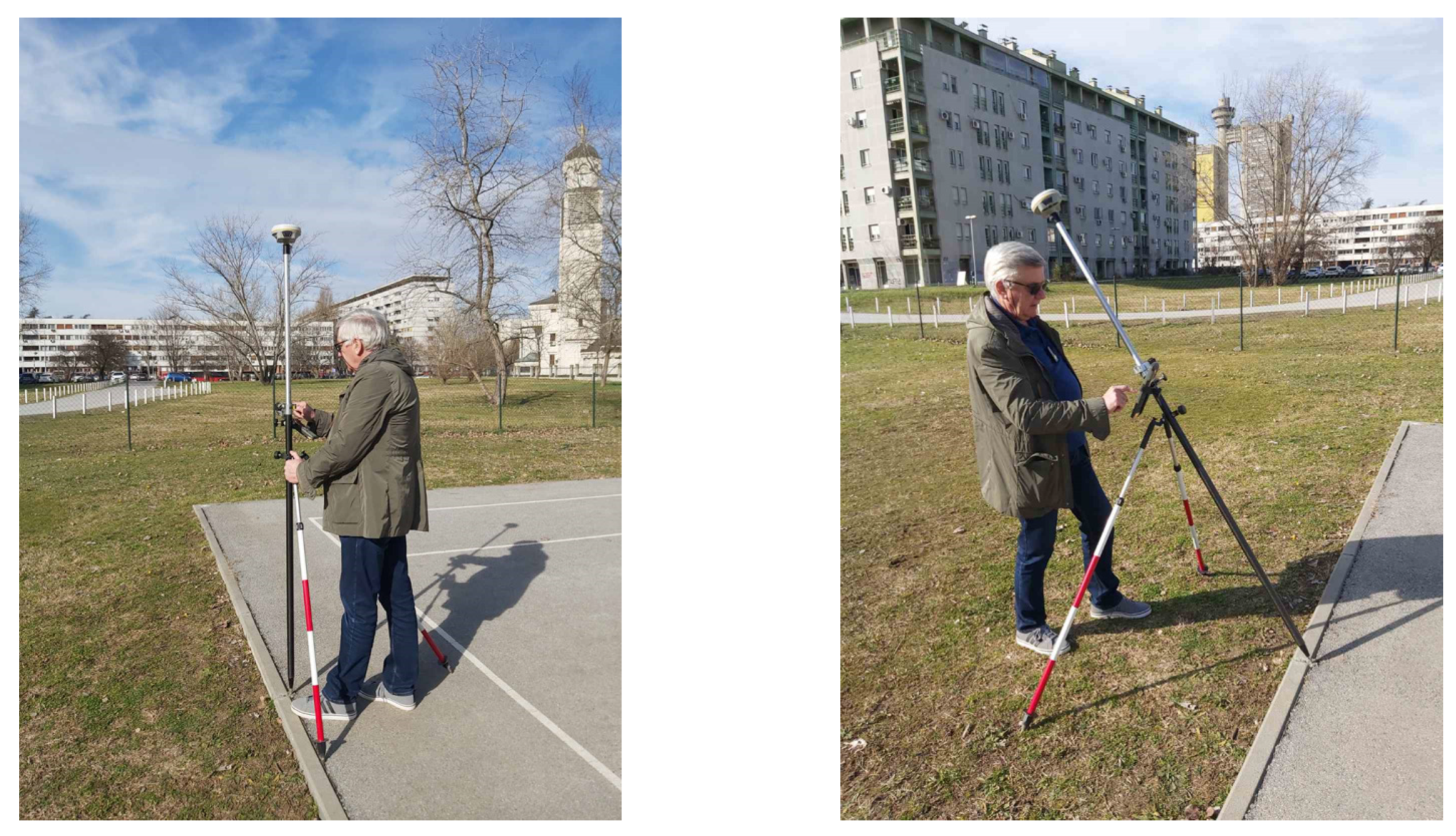
For the purpose of calculating the measurement uncertainty of the coordinates of the point of interest measured using the GNSS/IMU receivers with the tilt compensation function turned off/on, a new experiment was performed during the period of 3 months (from November 2023 until January 2024)—Figure 5.
Measurements were performed using seven different types of GNSS receivers and four different software support solutions. The list of receivers with support software and declared accuracy in RTK mode is shown in Table 2. All GNSS/IMU receivers were previously calibrated according to the procedure provided by the ISO 17123-8 standard and had the following parameters determined: deviations from the nominal values (), standard deviations of a single horizontal distance and experimental standard deviations of a single measurement of x, y (, ).
The GNSS/IMU calibration process starts by placing the GNSS receiver pole in its vertical direction at the test polygon reference point and with the tilt compensation function turned off. From the calibration results (Table 2), it was concluded that all GNSS/IMU receivers meet the accuracy of horizontal positioning, which is declared by the manufacturer.
In order to show the displacement of measurements in the tilt position from the POI (∆a), the distance between vertical projections of phase center on the ground for the vertical position and tilted position for the tilt angle α = 30° was calculated using Equation (5). In this experiment, the coordinate direction north–east was used with = 1 m. The authors decided to perform a set of measurements for GNSS receiver AlphaSurvey Alpha 4i, with a tilt angle of α = 45°, where = 1.41 m was calculated.
After the calibration of GNSS/IMU receivers on a test polygon of the accredited laboratory [27], a series of measurements were performed with the tilt compensation function turned on, using the procedure described in Section 3. of this paper.
Measurements in each of the five positions of the GNSS/IMU receivers with the tilt compensation function turned on () lasted up to 20 min. All the necessary measurements per each GNSS/IMU receiver were completed within a period of up to 120 min. The measurements were carried out according to the manufacturer’s instructions and the rules prescribed by the “Rulebook on the application of Global Navigation Satellite System technology in the areas of State Survey and Cadastre” [28] which is the bylaw governing the use of GNSSs in geodetic works in the Republic of Serbia. Deviations of coordinates x and y per series/positions of the measurements relative to the vertical position of the GNSS receiver (“Position C”) with the tilt compensation function turned on and α = 30° are shown in Table 3.
The combined uncertainty () of the coordinates of the point of interest was calculated using Equation (15). Values for typical influence quantities of GNSS RTK, for Equation (15), were taken from the ISO 17123-8:2015 standard: = 3.49 mm (specified by the manufacturer of GNSS receiver); = 0.29 mm; = 1 mm, = 1 mm, = 0.05 mm; , , = 1 mm; = 1 mm; and = 0.56 mm.
The standard uncertainties of a single position ( were calculated for each GNSS/IMU receiver separately, within the calibration process based on Equation (17). The experimental standard deviation of a single measurement of x and y (in an open sky environment had values that were lower than the declared standard uncertainty of the IMU component () (tilt compensation accuracy—Equation (18)), declared by the manufacturers of GNSS/IMU receivers.
For example, for the GNSS/IMU receiver Alpha5i, the following was calculated: = 4.62 mm. By entering this value in Equation (15) and by equalizing influence the value of 6.12 mm was calculated. For the IMU component, the value of the declared manufacturer tilt compensation accuracy was = 17 mm (Table 4).
Position errors 2D () for GNSS receiver Alpha5i calculated via Equation (19) were as follows:
Respectively, expanded uncertainty () calculated via Equation (20) was as follows:
The limit value for differences along the coordinate axes () calculated using Equation (22) for GNSS receiver Alpha5i was as follows:
Homogeneity testing in the direction of the coordinate axes and was analyzed according to the following criteria: the maximum deviation . If this criterion was met, the evaluation “Satisfactory” was achieved, otherwise it was marked as “Unsatisfactory” (Table 4).
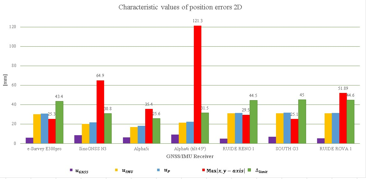
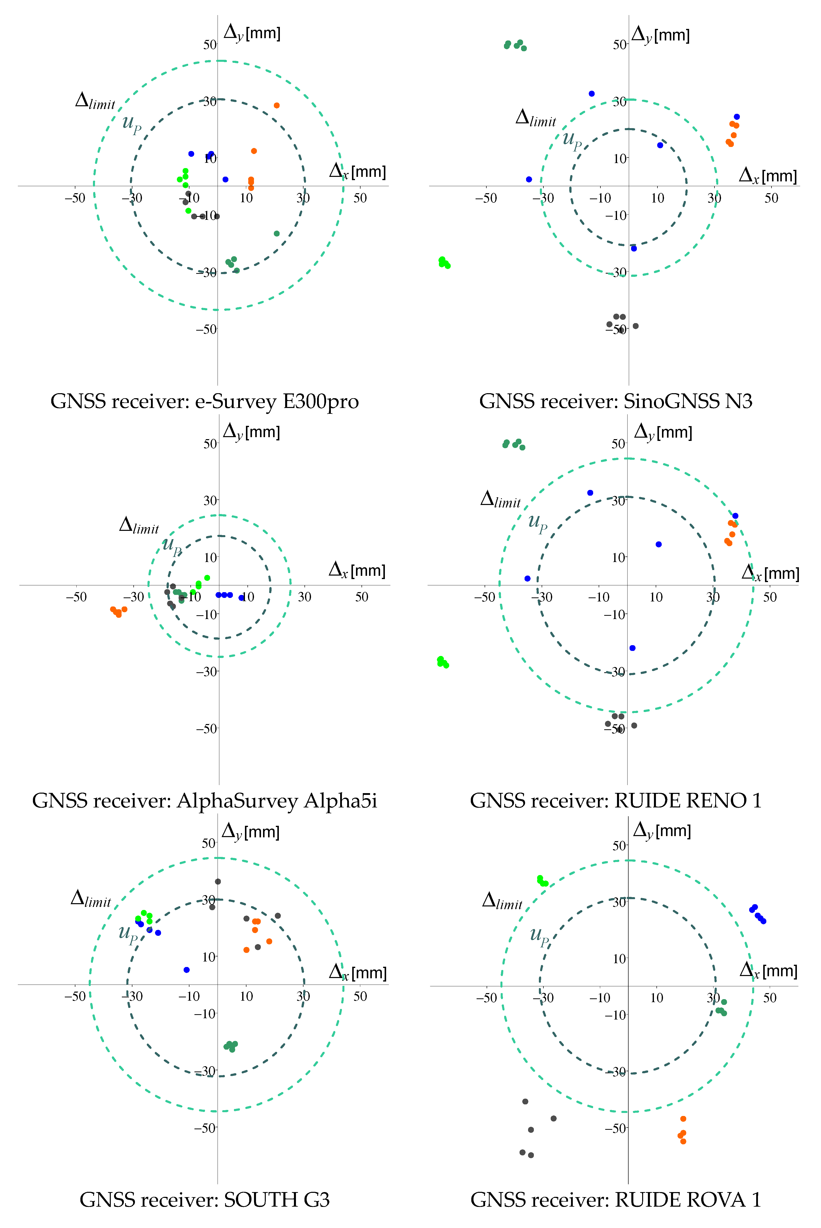
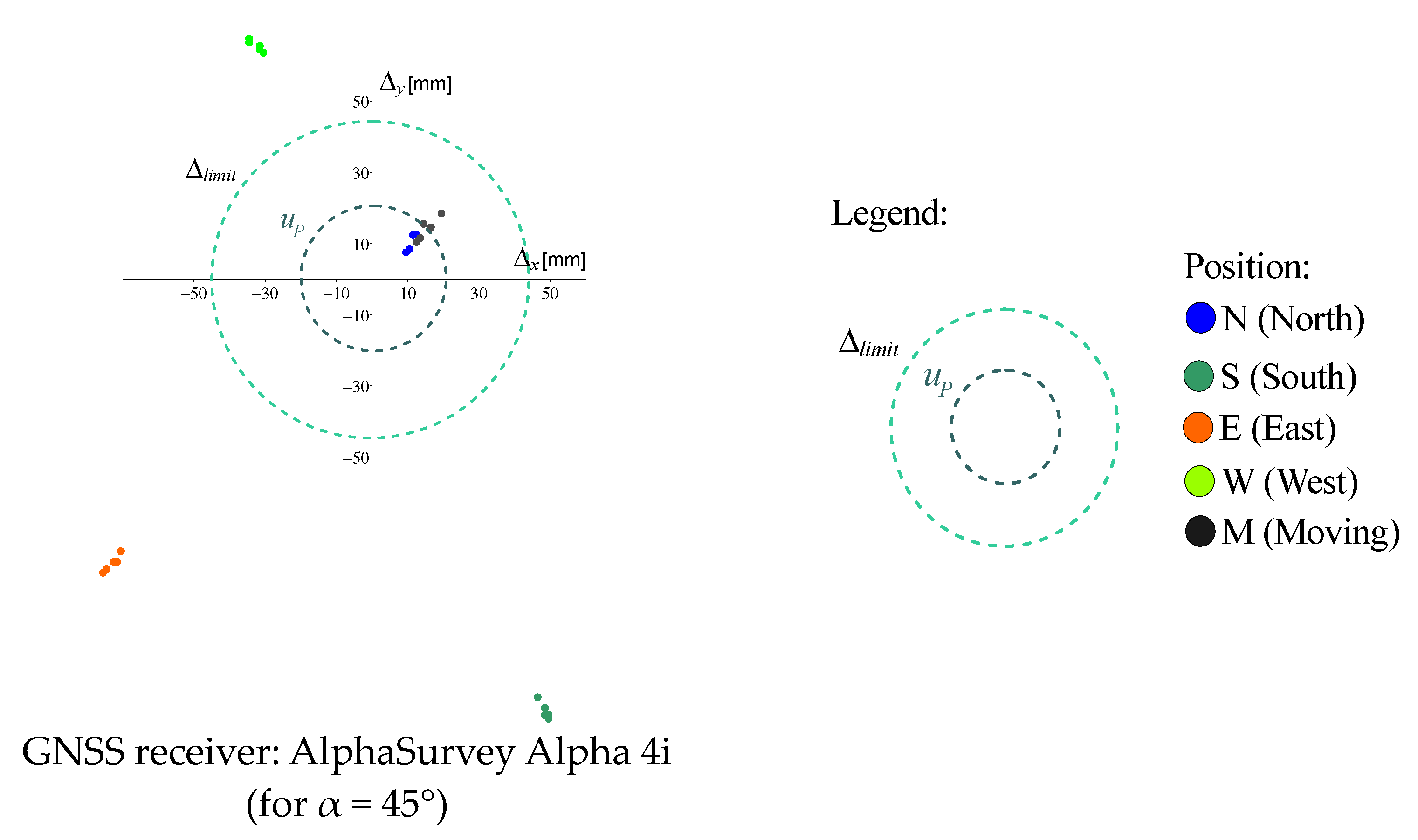
Repeatability as the lower limit of accuracy for the GNSS receivers used in the experiment is graphically shown in Figure 6.
A preliminary assessment of accuracy was performed for each GNSS/IMU receiver. This included an analysis of instrument performance, as shown in Table 2. Position errors 2D () were used as a reference and indicator for assessing the limit value for differences in all five measurement positions: N, S, E, W and M. Figure 6 presents an acceptable range for for each GNSS/IMU receiver used in the experiment. This serves as the basis for the discussion of the achieved results.
5. Discussion
Technological innovations in the production of GNSS receivers and antennas have enabled the use of GNSS/IMU equipment in geodetic RTK surveying. The increased number of GNSS satellites, advanced signal structure and application of sensors have enabled GNSS measuring in situations where it was not suitable before.
The use of tilt compensation technology is increasing rapidly, and for this reason, the practical limits of its use are under discussion. The authors of this paper had seven GNSS/IMU receivers available for the experiment. Measurements were performed with the same tilt compensation function in an open sky environment with the intention of checking the coordinate deviations on the point of interests that are part of the test polygon used for GNSS RTK calibration. Deviations in the direction of the coordinate axes are shown in Table 3. For a tilt of 30°, the maximum deviation was noted in the direction of the x-axis and was equal to −64.92 mm for GNSS receiver SinoGNSS N3. For a tilt of 45°, GNSS receiver AlphaSurvey Alpha 4i was examined, and the maximum deviation was noted in the direction of the y-axis and was equal to −121.3 mm. These deviations confirm the manufacturer’s instruction that GNSS/IMU receivers are best to be used with a tilt angle of up to 30°.
The experimental standard deviation of a single measurement of x and y in an open sky environment in the short baseline test polygon (distance ≤ 5 m) had values ≤ 5.57 mm (Table 2). For all used GNSS/IMU receivers, the standard uncertainties of GNSS coordinates of the antenna phase center are presented in Table 4, and they were within the range of for a tilt of 30°.
The standard uncertainty of the IMU component was within the range of . The pole tip position error was within the range of (Table 4). These values were calculated in the calibration process from a single measurement of x and y and used to calculate the limit value for the differences along the coordinate axes x and y. These limit values were within the range of . The GNSS/IMU receivers with characteristic values of position errors 2D marked as “Satisfactory” were e-Survey E300pro, RUIDE RENO 1 and SOUTH G3. In this way, the standard uncertainties of a single position (x, y) accuracy aspect of GNSS/IMU were determined, and the practical limits of using the tilt compensation technology of GNSS/IMU receivers were examined (Table 4).
6. Conclusions
In this paper are presented the results of an experiment that was conducted with the aim to determine the accuracy and reliability of seven GNSS/IMU receivers. Before carrying out the experiment, each GNSS receiver was calibrated, and the metrological characteristics of GNSS RTK were confirmed.
The monitoring of GNSS signals is of great importance, especially in situations where the tilt compensation function of GNSS/IMU receivers is to be used and in conditions of densely built-up areas. The authors of this paper work with a laboratory that is accredited according to the ISO 17025 standard and is in daily contact with distributors and users of geodetic equipment in the Republic of Serbia since the laboratory provides calibration services for total stations, levels and GNSS receivers. Purchasers of GNSS/IMU receivers look for answers to the following questions:
- For which tasks is the tilt compensation function most useful?
- What are the tasks that they cannot be used for?
The authors looked for answers to these questions in communication with distributors of GNSS receivers and with purchasers and users in the Republic of Serbia and also through available research in scientific works and publications of the professional community. Users of GNSS/IMU receivers emphasize its importance in increasing productivity for the cadastral surveying of large areas while using the tilt compensation function. The use of GNSS/IMU receivers with the tilt compensation function turned on is less tiring (data collection is faster), but the use of this measurement option is viable only in situations where the required coordinate accuracy is not better than 5 cm.
Users of GNSS/IMU receivers in the Republic of Serbia pointed out that sometimes they have problems when performing IMU initialization requests. Certain movements with the pole, walking in circles, swinging back and forth, or circular movements must be performed for IMU initialization. Once the GNSS/IMU receiver is initialized, the function of the IMU is not easily lost even if the GNSS receiver pole is carried on the shoulder, held horizontally or facing downwards. Since GNSS/IMU equipment manufacturers work on improvements of the tilt compensation function and lowering its cost, it is natural to expect that more and more of its users will choose this convenient feature, rather than GNSS receivers without IMU components installed.
The scientific and professional community emphasizes the importance of the calibration of geodetic equipment. Calibrations should be conducted in accredited laboratories and according to standard methods. The testing method of the GNSS/IMU receiver presented in this paper can help its users to make correct conclusions regarding the coordinate accuracy of the point of interest measured.
The conducted research can be used to check the internal accuracy and functionality of GNSS/IMU receivers in the permanent GNSS network stations. The use of different permanent GNSS networks has an impact on the accuracy, reliability and convergence time of obtaining the RTK solution. In the Republic of Serbia exists three permanent GNSS networks: AGROS (Active Geodetic Reference Network of Serbia) [29], “Vekom Net” [30] and “GentooARS” [31]. Each of them has different geographic distributions of reference points and uses different processing software. This means that GNSS RTK receivers connected to GNSS networks that have reference GNSS points near the POI will provide more accurate corrections in that region (correction information for satellite orbits, clock errors, ionospheric delay, etc.). Permanent GNSS networks have different detections and corrections for atmospheric effects, which affects the accuracy of RTK solutions [24]. In order to make these influences negligible, the entire experiment was performed by connecting the GNSS receivers to the same GNSS network, i.e., AGROS [29].
The performance of the used GNSS receivers is shown in Figure 6. All tested GNSS/IMU receivers are compatible with the correction format provided by the permanent GNSS networks of the Republic of Serbia. The external accuracy of the model can be checked by successively connecting it to available permanent GNSS networks. In this case, based on the research previously conducted by the author [32], it is justified to expect variable levels of coordinate accuracy.
Author Contributions
J.G. and S.D.: conceptualization, methodology, investigation, formal analysis, data curation, writing—original draft, writing—review and editing, visualization. O.V.Š.: methodology, investigation, formal analysis, data curation, writing—review and editing. All authors have read and agreed to the published version of the manuscript.
Funding
The research was conducted using the resources of the Association Transverzala Belgrade (112043118).
Data Availability Statement
Data are contained within the article.
Acknowledgments
Technical support for the experiment was provided by geodetic organizations of the Republic of Serbia whose GNSS receivers were calibrated in the Association Transverzala Belgrade.
Conflicts of Interest
The authors declare no conflicts of interest.
References
- Hofmann-Wellenhof, B.; Lichtenegger, H.; Wasle, E. GNSS—Global Navigation Satellite Systems: GPS, GLONASS, Galileo & More; Springer: Wien, Austria, 2008; 516p, ISBN 978-3-211-73012-6. [Google Scholar]
- Langley, R.B.; The Magnetic Compass and GPS. GPS World. 2003. Available online: http://gauss.gge.unb.ca/papers.pdf/gpsworld.september03.pdf (accessed on 5 November 2023).
- Luo, X.; Schaufler, S.; Richter, B. Leica GS18 T World’s Fastest GNSS RTK Rover; Leica Geosystems AG: Heerbrugg, Switzerland, 2018. [Google Scholar]
- Lin, H. High-precision RTK Positioning with Tilt, Compensation: Data Fusion Algorithm. In Proceedings of the 34th International Technical Meeting of the Satellite Division of The Institute of Navigation (ION GNSS+ 2021), St. Louis, MO, USA, 20–24 September 2021; Wuhan University: Wuhan, China, 2021. [Google Scholar]
- Chen, Q.; Lin, H.; Guo, R.; Niu, X. Rapid and accurate initial alignment of the low-cost MEMS IMU chip dedicated for tilted RTK receiver. GPS Solut. 2020, 24, 119. [Google Scholar] [CrossRef]
- Luo, X.; Schaufler, S.; Carrera, M.; Celebi, I. High-precision RTK positioning with calibration-free tilt compensation. In Proceedings of the FIG Congress 2018, Istanbul, Turkey, 6–11 May 2018. [Google Scholar]
- Muhammad, S. GNSS/INS Integration in Urban Areas; Department of Electronics and Telecommunications; Norwegian University of Science and Technology: Trondheim, Norway, 2014. [Google Scholar]
- Luo, X.; Chen, J.; Richter, B. How Galileo benefits high-precision RTK—What to expect with the current constellation. GPS World 2017, 28, 22–28. [Google Scholar]
- NovAtel Customer Service. GPS Position Accuracy Measures. NovAtel Positioning Leadership, APN-029, Rev 1. 2003. Available online: http://www.gisresources.com/wp-content/uploads/2014/03/gps_book.pdf (accessed on 21 March 2024).
- An, X.; Meng, X.; Jiang, W. Multi-constellation GNSS precise point positioning with multi-frequency raw observations and dual-frequency observations of ionospheric-free linear combination. Satell. Navig. 2020, 1, 7. [Google Scholar] [CrossRef]
- Urke, T. Accuracy of Tilt-Compensated GNSS-Sensors Using Network-RTK; Fakultet for Ingeniørvitenskap Institutt for Vareproduksjon og Byggteknikk; Noregs Teknisk-Naturvitskaplege Universitet: Trondheim, Norway, 2021. [Google Scholar]
- González-Calvo, M.; Luo, X.; Aponte, J.A.; Richter, B. Improved high-precision RTK positioning through multipath reduction and interference mitigation. In Proceedings of the FIG Congress. Volunteering for the Future—Geospatial Excellence for a Better Living, Warsaw, Poland, 11–15 September 2022. [Google Scholar]
- Specht, C.; Szot, T.; Specht, M.; Dąbrowski, P. Selected aspects of testing the positioning accuracy of GNSS receivers used in sports and recreation by dynamic measurements Balt. J. Health Phys. Act. 2019, 11, 75–84. [Google Scholar] [CrossRef]
- Yang, N.; Freestone, J. High-performance GNSS antennas with phase-reversal quadrature feeding network and parasitic circular array. In Proceedings of the ION GNSS+ 2016, Portland, OR, USA, 12–16 September 2016; pp. 364–372. [Google Scholar]
- Bojorquez-Pacheco, N.; Romero-Andrade, R.; Trejo-Soto, M.E.; Hernández-Andrade, D.; Nayak, K.; Vidal-Vega, A.I.; Arana-Medina, A.I.; Sharma, G.; Acosta-Gonzalez, L.E.; Serrano-Agila, R. Ocena delovanja eno in dvofrekvenčnih nizkocenovnih spreje-mnikov GNSS v statičnem relativnem načinu|Performance evaluation of single and double-frequency low-cost GNSS receivers in static relative mode. Geod. Vestn. 2023, 67, 235–248. [Google Scholar] [CrossRef]
- El-Hattab, A.I. Influence of GPS antenna phase center variation on precise positioning. NRIAG J. Astron. Geophys. 2013, 2, 272–277. [Google Scholar] [CrossRef]
- Rocken, C.; Meertens, C.; Stephens, B.; Braun, J.; VanHove, T.; Perry, S.; Ruud, O.; McCallum, M.; Richardson, J.; UNAVCO Academic Research Infrastructure (ARI) Receiver and Antenna Test Report. UNAVCO Boulder Facility International Report. Available online: https://www.unavco.org/projects/project-support/development-testing/publications/ari_test.pdf (accessed on 5 December 2023).
- Zhou, R.; Hu, Z.; Zhao, Q.; Cai, H.; Liu, X.; Liu, C.; Wang, G.; Kan, H.; Chen, L. Consistency Analysis of the GNSS Antenna Phase Center Correction Models. Remote Sens. 2022, 14, 540. [Google Scholar] [CrossRef]
- Heister, H. The new ISO standard 17123-8 for checking GNSS field measuring systems. In Proceedings of the FIG Working Week, Stockholm, Sweden, 14–19 June 2008. [Google Scholar]
- ISO 17123-8:2015; Optics and Optical Instruments—Field Procedures for Testing Geodetic and Surveying Instruments, Part 8: GNSS Field Meas-urement Systems in Real-Time Kinematic (RTK). ISO: Geneva, Switzerland, 2015.
- Mader, G.L. GPS Antenna Calibration at the National Geodetic Survey. GPS Solut. 1999, 3, 50–58. [Google Scholar] [CrossRef]
- Prešeren, P.P.; Mencin, A.; Stopar, B. Analiza preizkusa instrumentarija gnss-rtk po navodilih standarda iso 17123-8.|Analysis of gnss-rtk instruments testing on the iso 17123-8 instructions. Geod. Vestn. 2010, 54, 607–626. [Google Scholar] [CrossRef]
- Ignjatović Stupar, D.; Ogrizović, V. Using single frequency receivers for future cubesat GPS-RO missions. In Proceedings of the 6th International Conference, Subotica, Serbia, 20 April 2018. [Google Scholar] [CrossRef]
- Li, J.; Li, F.; Liu, L.; Huang, L.; Zhou, L.; He, H. A CalibratedGPT3 (CGPT3) Model for the Site-Specific Zenith Hydrostatic Delay Estimation in the Chinese Mainland and Its Surrounding Areas. Remote Sens. 2022, 14, 6357. [Google Scholar] [CrossRef]
- Trimble Announces Calibration-Free Tilt Compensation for Their Flagship GNSS Rover. Available online: https://www.geospatialworld.net/blogs/trimble-announces-calibration-free-tilt-compensation-for-their-flagship-gnss-rover/ (accessed on 7 December 2023).
- Gučević, J.; Delčev, S.; Kuburić, M.; Trifković, M.; Ogrizović, V. Impact of Vial Bubble on the Accuracy of Positions in the GNSS-RTK Mode. Tech. Gaz. 2022, 29, 1230–1235. [Google Scholar] [CrossRef]
- Available online: http://www.registar.ats.rs/predmet/1323/ (accessed on 2 November 2023).
- Pravilnik o Primeni Tehnologije Globalnog Navigacionog Satelitskog Sistema u Oblastima Državnog Premera i Katastra, “Službeni Glasnik RS”, br. 72/2017. Available online: http://demo.paragraf.rs/demo/combined/Old/t/t2017_07/t07_0328.htm (accessed on 10 November 2023).
- AGROS. Available online: https://agros.rgz.gov.rs/ (accessed on 25 March 2024).
- Vekom Net. Available online: https://vekom.com/o-vekomnet-mrezi/ (accessed on 25 March 2024).
- GentooARS. Available online: http://www.geosolutions.co.rs/resenjeGeotaurNet.pdf (accessed on 25 March 2024).
- Gučević, J.; Vasović Šimšić, O.; Delčev, S.; Kuburić, M. Testing of Homogeneity of Coordinates of Various Permanent GNSS Reference Stations Networks of the Republic of Serbia According to the Common Requirements for Proving Competence. Sensors 2022, 22, 7867. [Google Scholar] [CrossRef] [PubMed]
Figure 1.
“Basic data processing schematic of the IMU-based tilted RTK receiver” [5].
Figure 1.
“Basic data processing schematic of the IMU-based tilted RTK receiver” [5].

Figure 2.
Accuracy versus precision [9].
Figure 2.
Accuracy versus precision [9].

Figure 3.
(a) GNSS receiver pole “Position C”—tilt compensation function is turned off; (b) GNSS receiver pole “Position N” and “Position S”—tilt compensation function is turned on; (c) GNSS receiver pole “Position E” and “Position W”—tilt compensation function is turned on; (d) GNSS receiver pole conical moving “Position M”—tilt compensation function is turned on.


Figure 4.
The principle of tilt compensation function of GNSS/IMU receiver.

Figure 5.
Measurements performed on a test polygon for calibration of GNSS RTK receivers [28].
Figure 5.
Measurements performed on a test polygon for calibration of GNSS RTK receivers [28].

Figure 6.
Graphical representation: position errors ; the limit value for differences ) along coordinate axes and deviation of coordinates and for each GNSS/IMU receiver.
Figure 6.
Graphical representation: position errors ; the limit value for differences ) along coordinate axes and deviation of coordinates and for each GNSS/IMU receiver.


Table 1.
Position accuracy measures [9].
Table 1.
Position accuracy measures [9].
| Accuracy Measures | Formula | Probability | Definition |
|---|---|---|---|
| DRMS | 65% | The square root of the average of the squared horizontal position errors. | |
| 2DRMS | 95% | Twice the DRMS of the horizontal position errors. | |
| MRSE | 61% | The radius of the sphere centered at the true position, containing the position estimate in 3D with a probability of 61%. |
Table 2.
Calibration results of GNSS/IMU receiver with the tilt compensation function turned OFF.
| GNSS Receiver/ Software Support | Horizontal/ Vertical Accuracy | Tilt Compensation Accuracy (mm) | (mm) | (mm) |
|---|---|---|---|---|
| e-Survey E300pro/ SurPad 4.2 | 8 mm + 1 ppm/ 15 mm + 1 ppm | 30 | −0.04 ± 0.59 | 2.15 3.68 |
| SinoGNSS N3/ Survey Master | 8 mm + 0.5 ppm/ 15 mm + 0.5 ppm | 20 | −0.57 ± 0.86 | 5.00 5.57 |
| AlphaSurvey Alpha5i/ Alpha DiMap Pro | 8 mm + 1 ppm/ 15 mm + 1 ppm | 8 + 0.3·tilt | −2.64 ± 1.35 | 2.94 3.57 |
| AlphaSurvey Alpha4i/ Alpha DiMap Pro | 8 mm + 1 ppm/ 15 mm + 1 ppm | 8 + 0.3·tilt | 1.20 ± 0.78 | 2.97 2.37 |
| RUIDE RENO 1/ Surv X | 8 mm + 1 ppm/ 15 mm + 1 ppm | 10 + 0.7·tilt | 0.24 ± 0.55 | 1.43 2.57 |
| SOUTH G3/ Surv X | 8 mm + 0.5 ppm/ 15 mm + 0.5 ppm | 10 + 0.7·tilt | −1.61 ± 1.31 | 4.04 3.69 |
| RUIDE ROVA 1/ Surv X | 8 mm + 1 ppm/ 15 mm + 1 ppm | 10 + 0.7·tilt | −1.38 ± 0.67 | 1.67 2.67 |
Table 3.
Deviation of coordinates x and y per series/positions of measurements relative to the vertical position of the GNSS/IMU receiver.
Table 3.
Deviation of coordinates x and y per series/positions of measurements relative to the vertical position of the GNSS/IMU receiver.
| Deviation of Coordinates per Series | [mm] | [mm] | [mm] | [mm] | [mm] |
|---|---|---|---|---|---|
| GNSS receiver: | e-Survey E300pro | ||||
| x-axis | −2.87 | 8.33 | 13.73 | −11.87 | −7.07 |
| y-axis | 9.33 | −25.27 | 8.73 | 3.33 | −8.07 |
| GNSS receiver: | SinoGNSS N3 | ||||
| x-axis | 0.50 | −39.90 | 36.28 | −64.92 | −2.76 |
| y-axis | 10.32 | 49.48 | 18.26 | −26.88 | −48.02 |
| GNSS receiver: | AlphaSurvey Alpha 5i | ||||
| x-axis | 2.60 | −13.60 | −35.40 | −7.00 | −16.20 |
| y-axis | −3.60 | −3.40 | −9.20 | 0.20 | −4.20 |
| GNSS receiver: | AlphaSurvey Alpha 4i (for α = 45°) | ||||
| x-axis | 11.50 | 48.50 | −72.90 | −32.50 | 15.30 |
| y-axis | 10.50 | −121.30 | −79.90 | 65.50 | 14.10 |
| GNSS receiver: | RUIDE RENO 1 | ||||
| x-axis | −2.80 | 31.00 | 28.00 | −17.60 | 5.60 |
| y-axis | 29.53 | −22.87 | 19.53 | −21.87 | −22.07 |
| GNSS receiver: | SOUTH G3 | ||||
| x-axis | −22.07 | 4.73 | 13.73 | −25.07 | 8.73 |
| y-axis | 17.20 | −21.60 | 18.20 | 23.40 | 24.80 |
| GNSS receiver: | RUIDE ROVA 1 | ||||
| x-axis | 45.69 | 32.84 | 18.96 | −30.56 | −33.80 |
| y-axis | 25.36 | −8.16 | −51.89 | 37.29 | −51.40 |
Table 4.
Characteristic values of position errors 2D.
| GNSS/IMU Receiver | [mm] | [mm] | [mm] | Evaluation | ||
|---|---|---|---|---|---|---|
| e-Survey E300pro | 5.8 | 30 | 30.6 | 25.3 | 43.4 | “Satisfactory” |
| SinoGNSS N3 | 8.5 | 20 | 21.7 | 64.9 | 30.8 | “Unsatisfactory” |
| Alpha5i | 6.1 | 17 | 18.1 | 35.4 | 25.6 | “Unsatisfactory” |
| Alpha4i (tilt 45º) | 9.0 | 21.5 | 22.2 | 121.3 | 31.5 | “Unsatisfactory” |
| RUIDE RENO 1 | 5.0 | 31 | 31.4 | 29.5 | 44.5 | “Satisfactory” |
| SOUTH G3 | 6.8 | 31 | 31.7 | 25.1 | 45.0 | “Satisfactory” |
| RUIDE ROVA 1 | 5.1 | 31 | 31.4 | 51.89 | 44.6 | “Unsatisfactory” |
Disclaimer/Publisher’s Note: The statements, opinions and data contained in all publications are solely those of the individual author(s) and contributor(s) and not of MDPI and/or the editor(s). MDPI and/or the editor(s) disclaim responsibility for any injury to people or property resulting from any ideas, methods, instructions or products referred to in the content. |
© 2024 by the authors. Licensee MDPI, Basel, Switzerland. This article is an open access article distributed under the terms and conditions of the Creative Commons Attribution (CC BY) license (https://creativecommons.org/licenses/by/4.0/).
Share and Cite
MDPI and ACS Style
Gučević, J.; Delčev, S.; Vasović Šimšić, O. Practical Limitations of Using the Tilt Compensation Function of the GNSS/IMU Receiver. Remote Sens. 2024, 16, 1327. https://doi.org/10.3390/rs16081327
AMA Style
Gučević J, Delčev S, Vasović Šimšić O. Practical Limitations of Using the Tilt Compensation Function of the GNSS/IMU Receiver. Remote Sensing. 2024; 16(8):1327. https://doi.org/10.3390/rs16081327
Chicago/Turabian StyleGučević, Jelena, Siniša Delčev, and Olivera Vasović Šimšić. 2024. "Practical Limitations of Using the Tilt Compensation Function of the GNSS/IMU Receiver" Remote Sensing 16, no. 8: 1327. https://doi.org/10.3390/rs16081327
Note that from the first issue of 2016, this journal uses article numbers instead of page numbers. See further details here.