
VLF Signal Noise Reduction during Intense Seismic Activity: First Study of Wave Excitations and Attenuations in the VLF Signal Amplitude


Abstract
1. Introduction
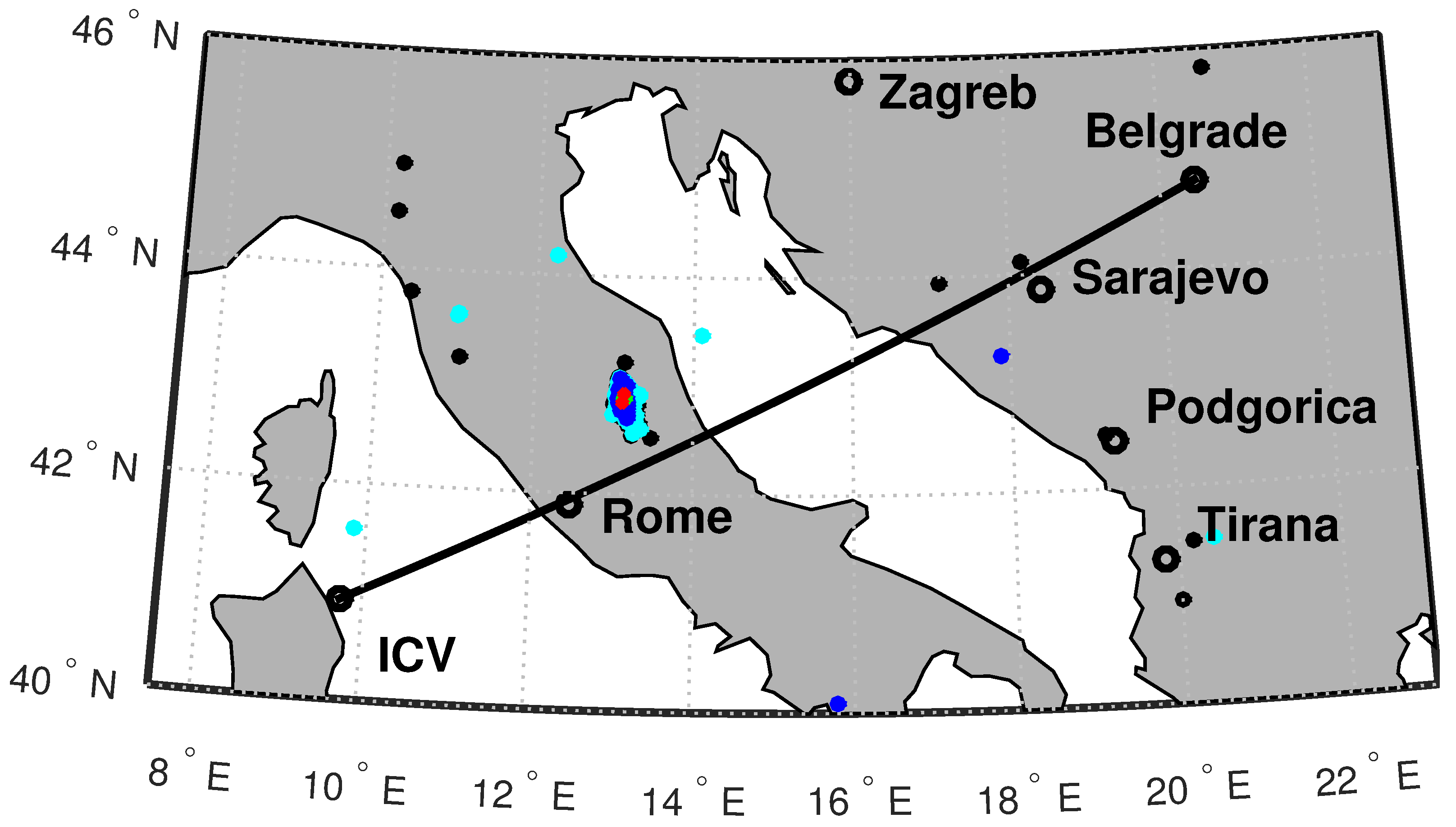
2. Observations
3. Data Processing
3.1. Input Data
- In which the amplitude values were too low (this indicated the absence of ICV signal detection). This process was carried out for all shown analyses.
- Around the amplitude minima that are characteristic during sunrise and sunset. These data were only eliminated in cases where the increase in was significant and only in determining the mean daily values of the considered parameters.
3.2. Frequency Domain
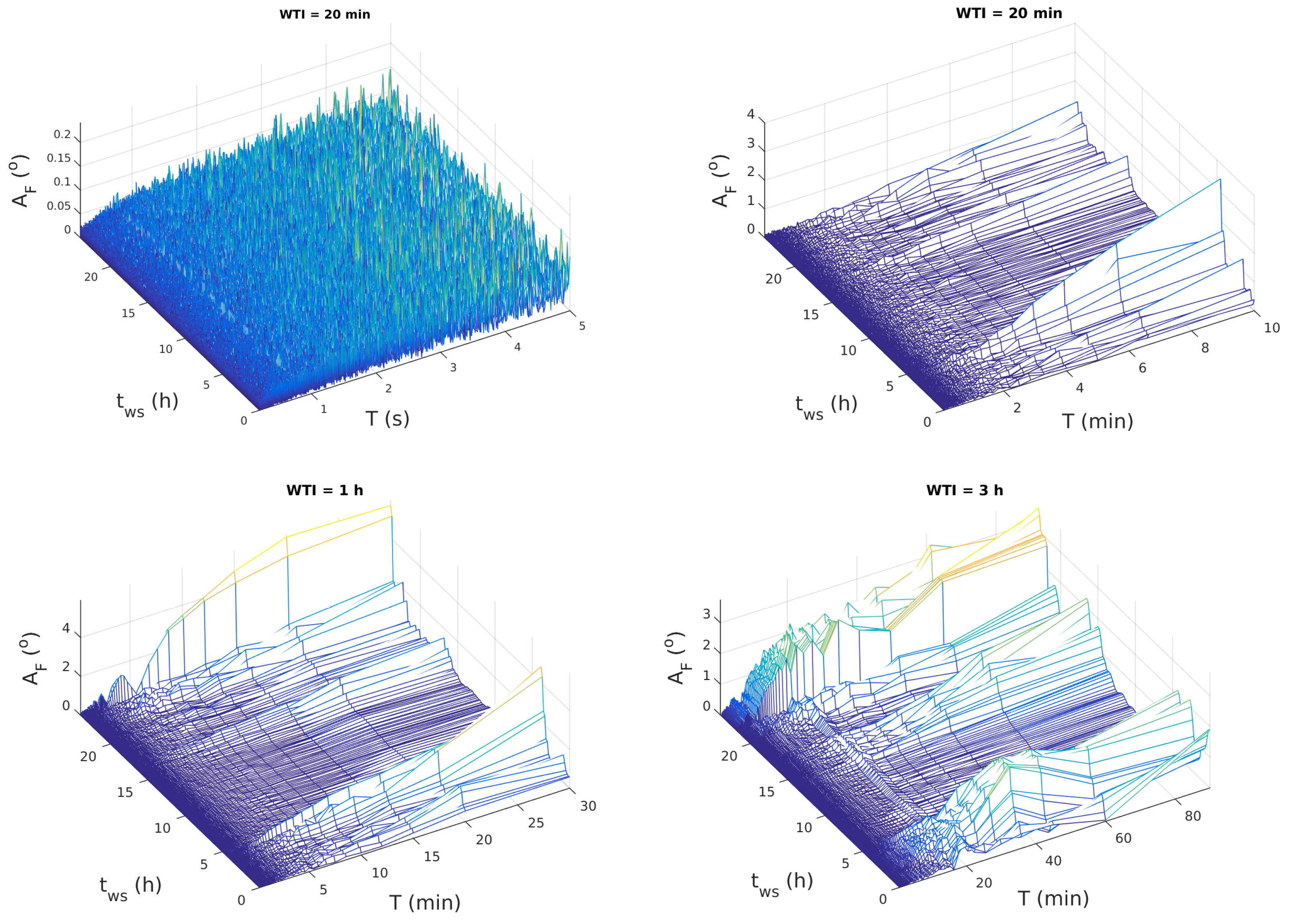
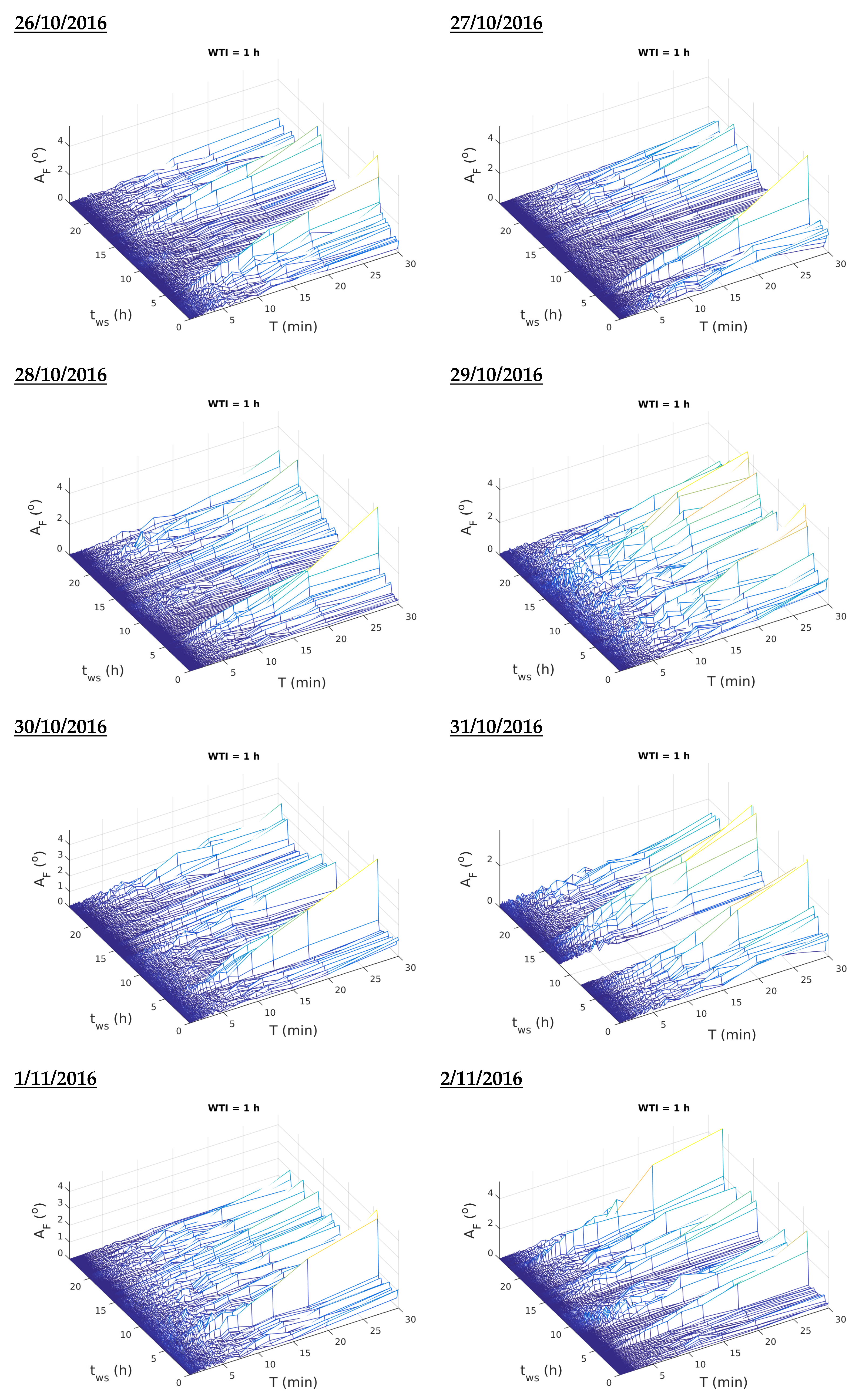
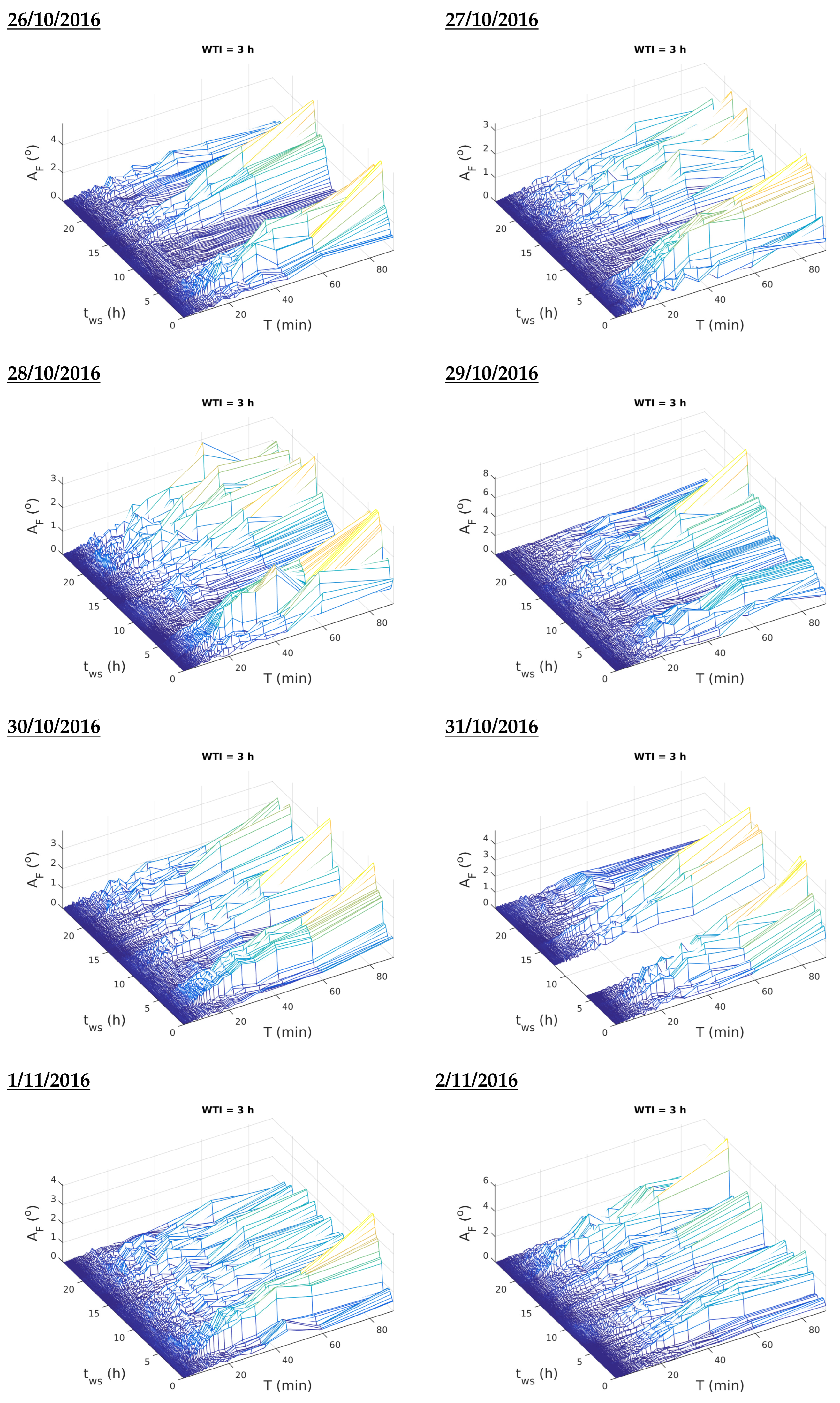
- Ten minutes in all three cases in 3D representations of the dependence;
- Twenty minutes for analyses based on determining mean values in 20 min intervals (so all recorded data were included in the analysis, and due to the non-overlapping WTIs, a single value was included in the mean value representing only one WTI).
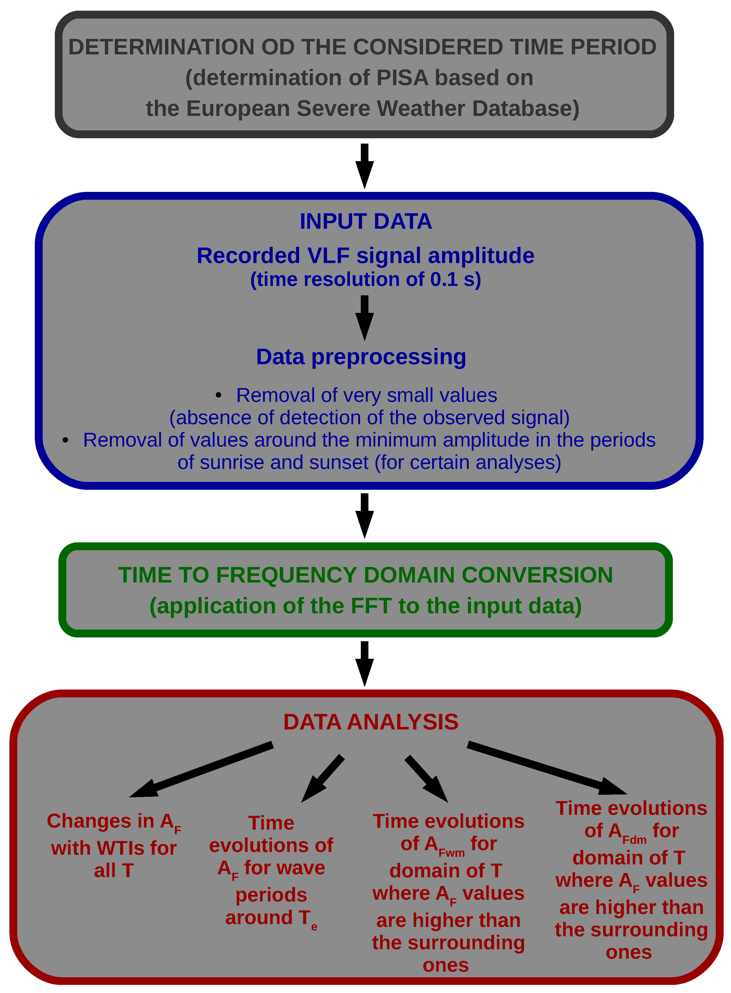
3.3. Data Analysis
- Visualisation of the changes in with WTIs which are represented by the times of their beginnings for all values of T. The error in the determination of is equal to the time resolution of the recorded data (0.1 s). Bearing in mind that it is significantly smaller than the value of , it can be considered approximately negligible. This also applies to other analyses in which this parameter is used. In the case of an error in the determination of T, there are two cases that depend on the values of T. This explanation is given in [30] and is based on the fact that by applying the FFT to data recorded at equidistant time intervals, equidistant values of f are obtained. Given that , the distance between neighbouring values of T increases with it. The distance for small values of T can be calculated as where and has values of 8.3333 × Hz, 2.7778 × Hz, and 9.2593 × Hz for WTIs of 20 min, 1 h, and 3 h, respectively. The error for the higher periods is determined by the absolute difference between a certain value of T and the first larger discrete value of this parameter. In this study, only a visual analysis was performed for higher values of T, so that error was only determined in the first way.
- Analysis of in WTIs starting at for wave periods around values of for which wave excitations are visible around the time of earthquakes that occurred during PWISA. We performed analyses for all values of that are specified in [30]: 0.2000 s, 0.2333 s, 0.3500 s, 0.4677 s, 0.7001 s, and 1.400 s. In order to take into account the possibility of more significant changes in very close periods, we considered the maximum value of values for the considered and for 5 of its closest larger and smaller values in WTI starting at :where is the ordinal position assigned to the element that represents in the data array for T. Taking into account the analysis of the error in the determination of T in the previous point and the fact that this analysis is relevant for WTI = 20 min, it can be approximately assumed that in this case, s, where is expressed in s.
- Analysis of the mean values of in WTIs starting at in the domain of T for which higher values are observed compared to the surrounding ones. This parameter was calculated as follows:where N is the total number of values in the considered WTI for the chosen T domain, and i is the ordinal position of a particular value in this array.
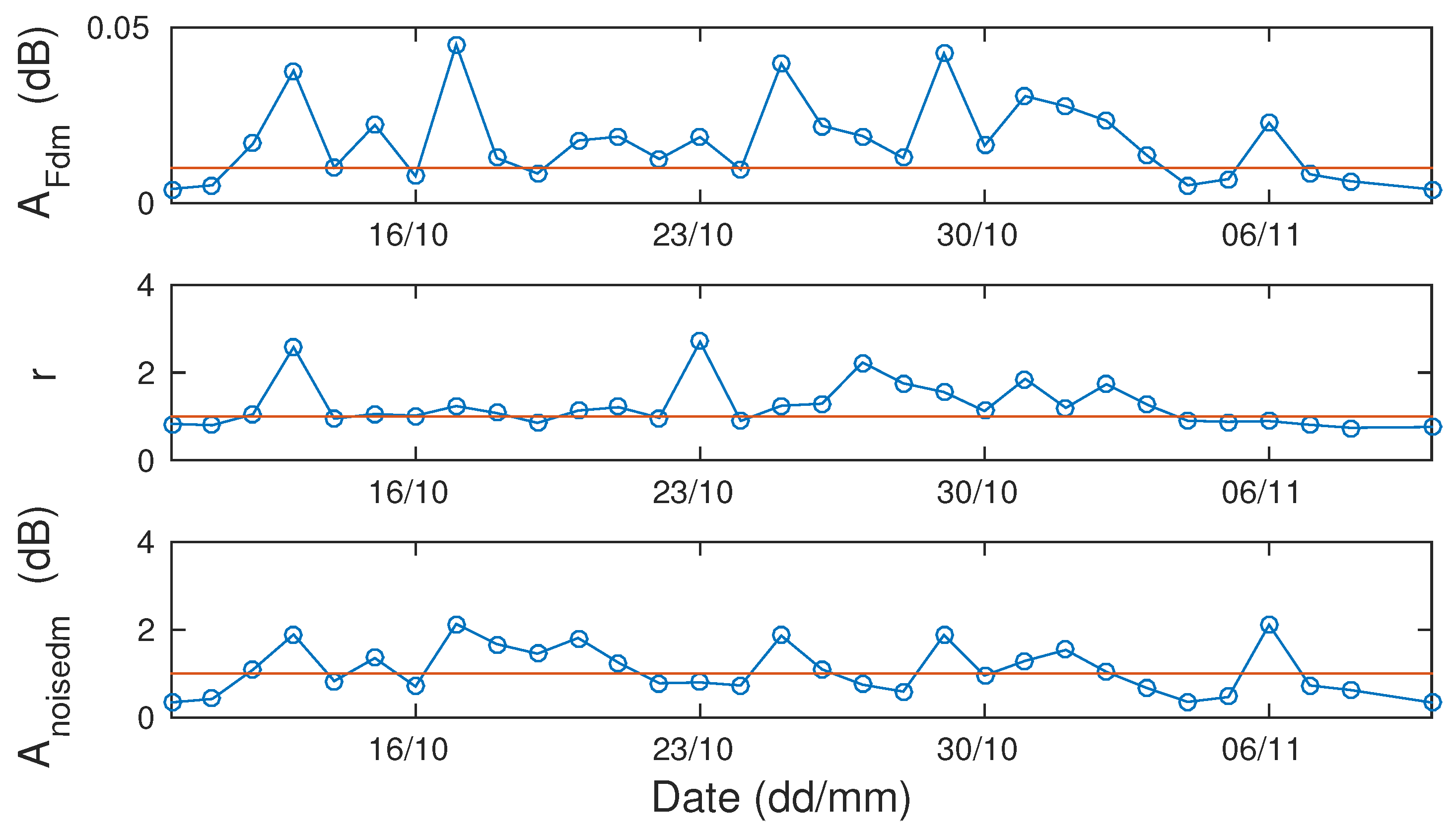
- Analysis of the time evolution of daily averaged values of in the domain of T for which higher values are observed compared to the surrounding ones. This parameter was calculated by the following expression:where D is the total number of relevant values in the considered day, and j is the ordinal position of a particular value in this array. We emphasise here that incorrect data were not considered in the respective analyses, so that D was not the same for all days. The analyses were performed both for its absolute values in the considered T domain and for its corresponding relative values r in relation to the reference domain with Fourier amplitude :In this way, we analysed the localisation of the observed differences, which is significant because, as seen in Section 4, in some cases, it is clearly visible, while in others, it is not. From this, we can conclude that the corresponding changes in the value of over time have different causes.
4. Results and Discussion
4.1. Quiet Conditions
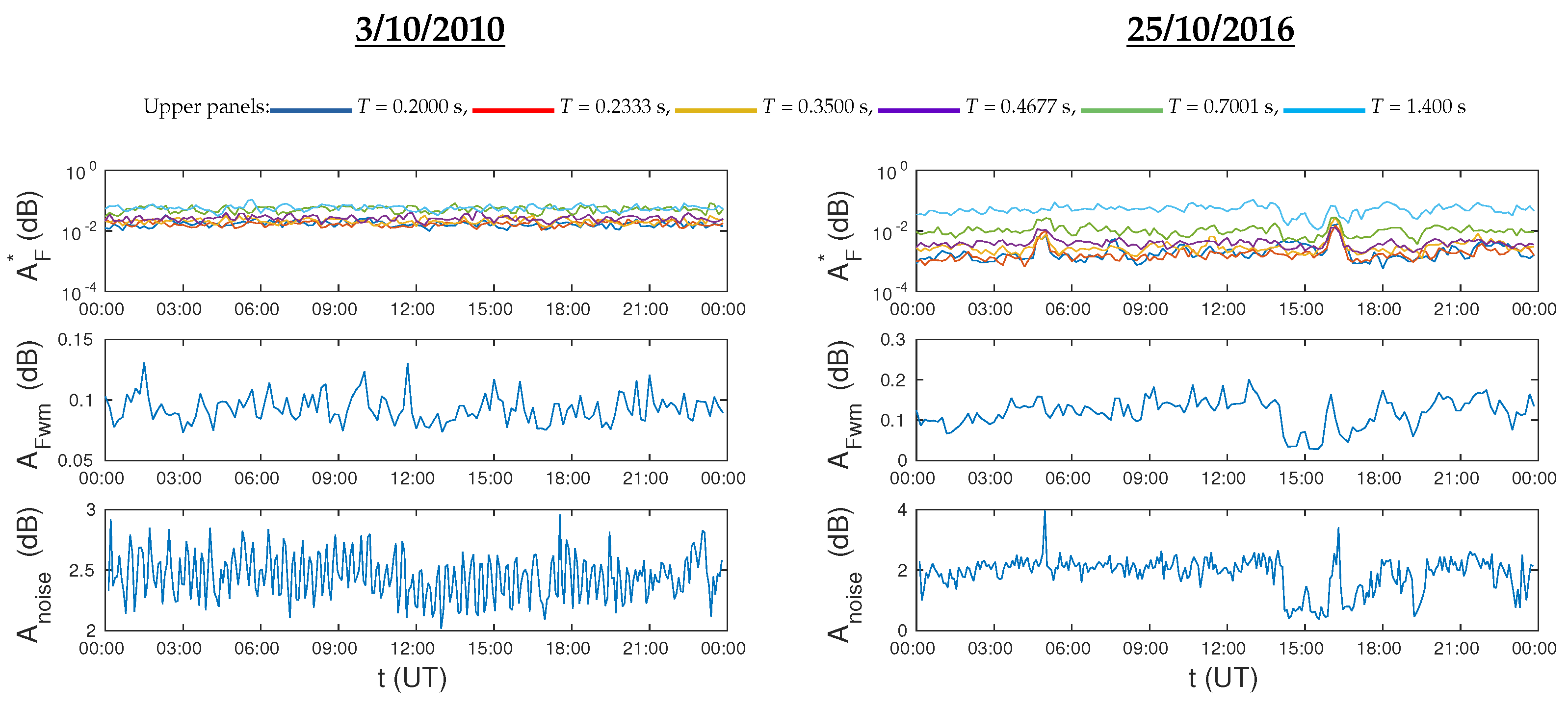
- On 3 October 2010, when the conditions were quiet and not a single earthquake was recorded.
- On 25 October 2016 (the day before the analysed period), during which the amplitude noise was stable with values around 2 dB except for a short period during the afternoon when an earthquake of magnitude ML 3.9 occurred in Central Italy [29].
4.1.1. First Reference Day: 3 October 2010
4.1.2. Second Reference Day: 25 October 2016
4.1.3. Comparisons of the Time Evolutions of for Narrow Domains of T during the Observed Reference Days
- Upper panels: Maximum values for each for six sets of 11 discrete T values determined around the values 0.2000 s, 0.2333 s, 0.3500 s, 0.4677 s, 0.7001 s, and 1.400 s, respectively (these values and their five closest lower and higher values). Based on the explanation in Section 3, s for the given T in these analyses are 0.0002 s, 0.0003 s, 0.0006 s, 0.001 s, 0.003 s, and 0.009 s, respectively.
- Middle panels: mean values for T between 1.4 s to 2 s for each .
- Bottom panels: the time evolutions of given in [29].
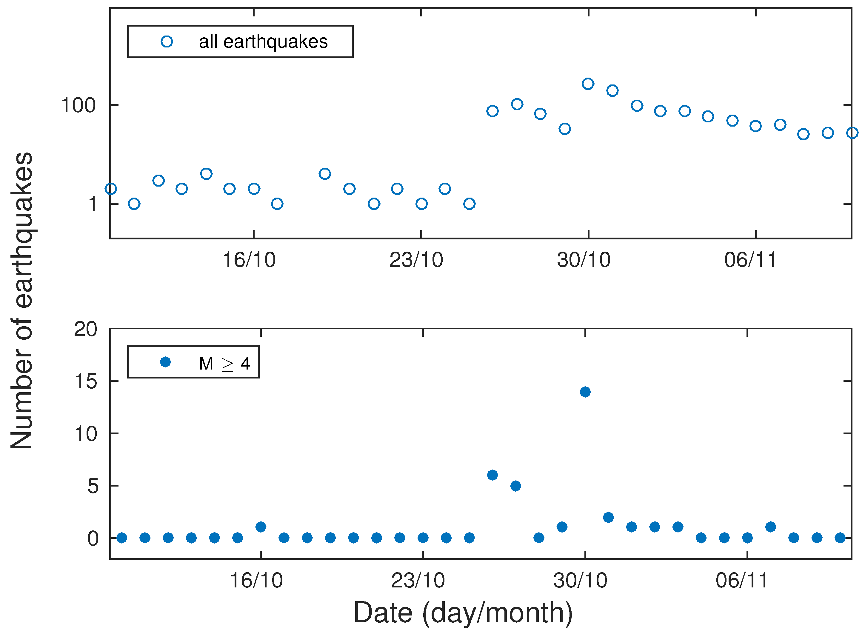
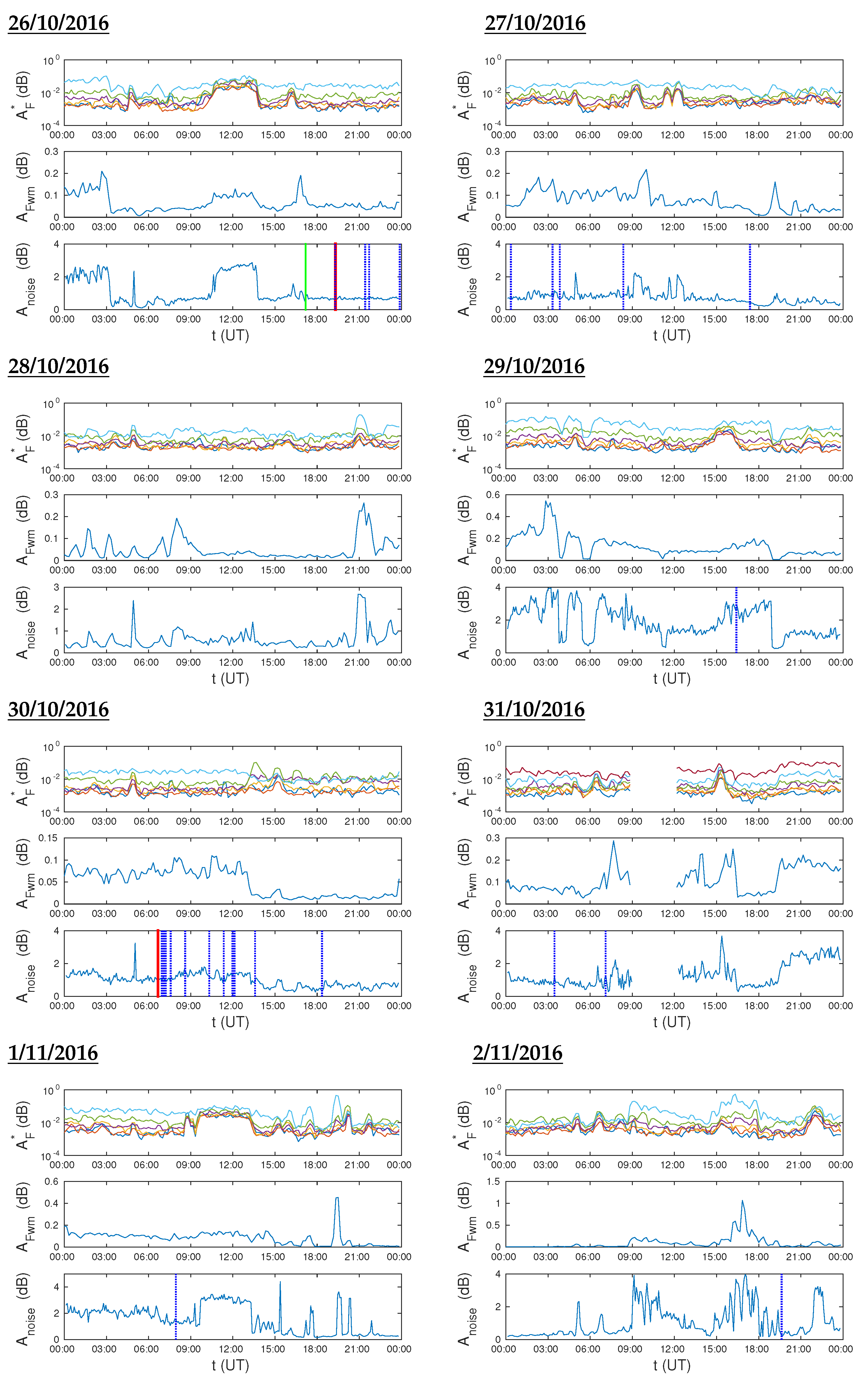
4.2. Seismic Active Period
- The data in the period 9:00 UT–12:20 UT on 31 October were not processed in all analyses, as no ICV signal was detected in that period. This can be seen from the time evolution of its amplitude which is shown in [29]. For the same reason, the data from parts of several days that were considered for examining the beginnings and ends of multi-day changes were removed.
- In the case of an increased , the recorded data in the periods of sunrise and sunset were not taken into account in the analyses of the daily values of and .
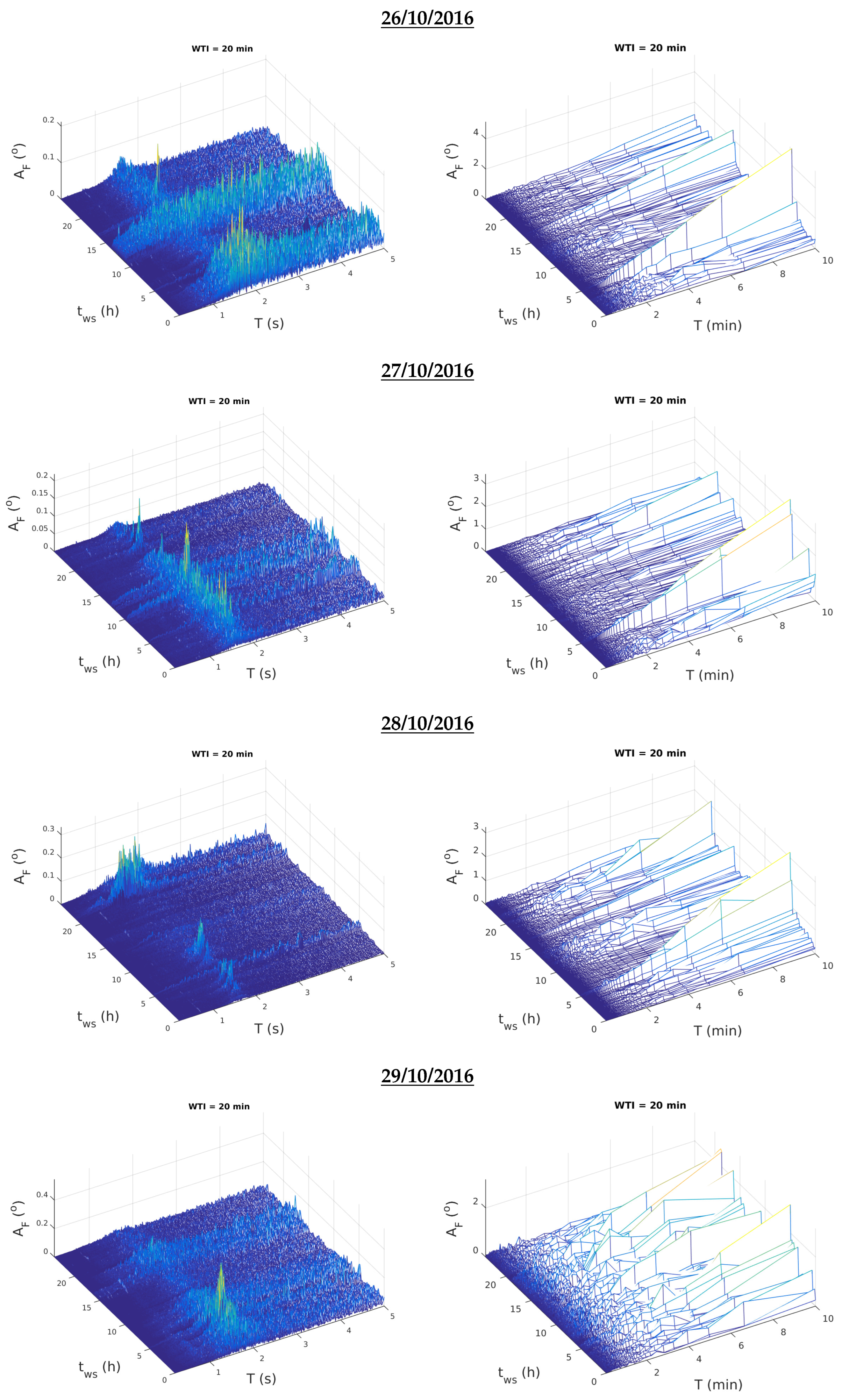
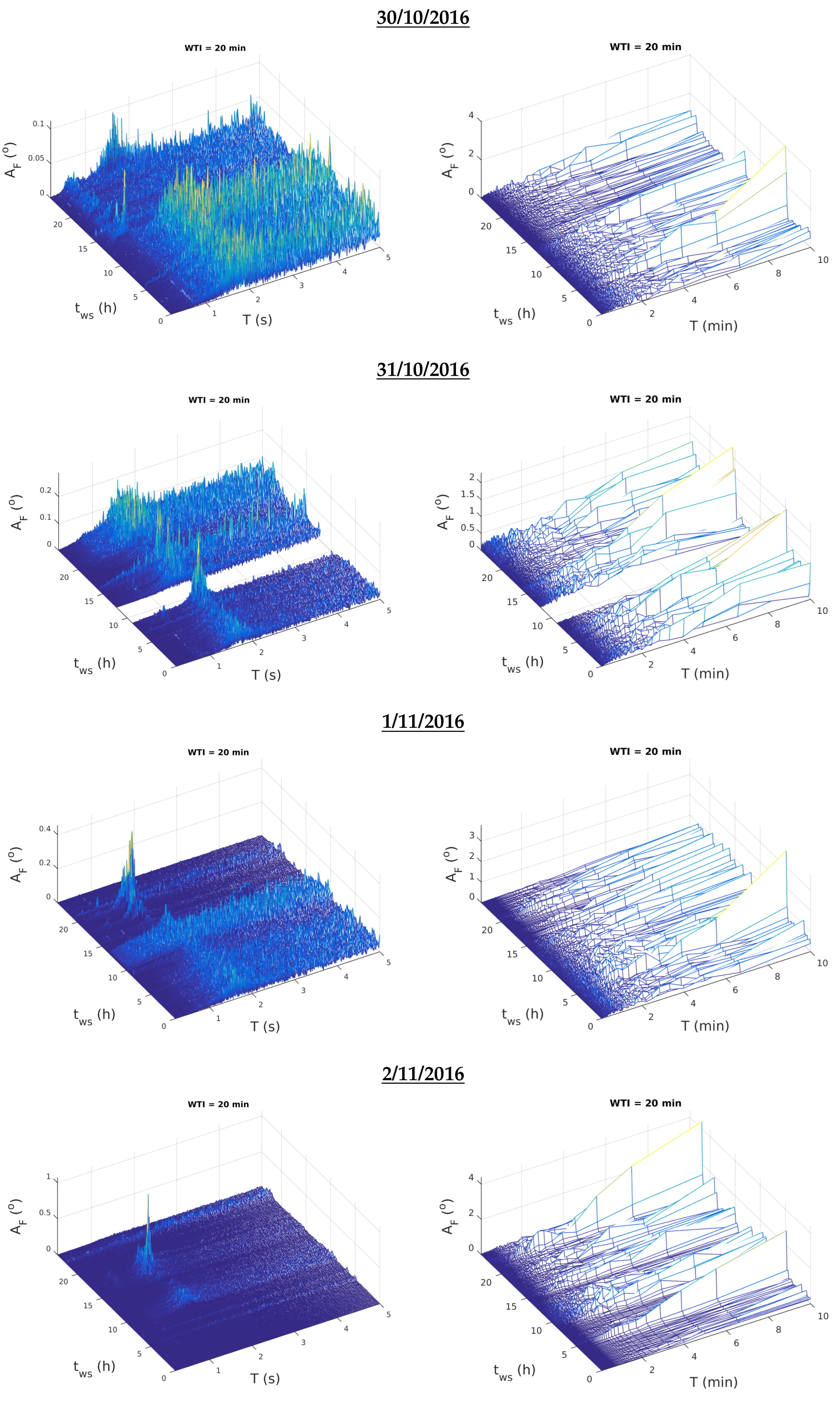
4.2.1. Small Wave Periods
- The existence of wave excitations at of 0.2333 s, 0.3500 s, 0.4677 s, 0.7001 s, and 1.400 s, which were visible in the cases of the previously analysed earthquakes that occurred during PWISA;
- Values of for the domain T from 1.4 s to 2 s, which were higher than other close values of T on almost all days from 26 October to 1 November;
- Attenuations of the waves at low wave periods.
- With the exception of time intervals of a few hours on 26, 29, and 31 October and on 1 November, the values for 2 s s were significantly lower than the values given for the reference days in Figure 4 and Figure 5. During the isolated intervals, was approximately equal to the values recorded on quiet days (see [29] and Figure 8).
- Although it is not noticeable on the 3D graphs due to the significantly smaller values of compared to their maximum, the values of this parameter for a small T were about an order of magnitude smaller than the values recorded on the first reference day (3 October 2010), which was also true for the values recorded on 25 October 2016 (the second reference day). This can be clearly seen in Figure 8.
- When the values were small in the periods of sunrise and sunset, smaller increases in were observed for T≤ 5 s in the short term.
4.2.2. Medium and Large Wave Periods
4.3. Analysis of the Reliability of the Relationship between Recorded Signal Changes and Seismic Activity and Possible Influences of Other Phenomena
- Earthquake characteristics (characteristics of the location where it occurred, the depth at which it occurred, its magnitude);
- The occurrence of other earthquakes (near the epicentre of the observed earthquake or at distant locations that are also near the propagation path of the observed signal) and their characteristics;
- The epicentre position in relation to the propagation path of the observed signal (their mutual distance, the epicentre position in relation to the considered transmitter and receiver);
- The state of the atmosphere during the analysed period;
- Characteristics of the observed signal, including parameters relevant to the observed transmitters and receivers.
- Phase I: diagnostics of changes that can be regarded as potential precursor of an earthquake given the defined characteristics of the recorded parameters.
- Phase II: determining the parameters that characterise these changes based on the smaller number of earthquakes in the case of PWISA, or the smaller number of PISAs, and the appropriate criteria to distinguish them from other potentially similar changes caused by other phenomena.
- Phase III: analysis of these parameters and criteria using a statistically significant number of appropriate samples for one signal.
- Phase IV: appropriate statistical analyses for several transmitters and receivers, which should (a) verify the results obtained in the previous phase and reveal possible differences for different signals and receivers and (b) provide detailed analyses of the observed changes in space.
5. Conclusions
- A reduction in the VLF signal amplitude and phase noises;
- The detection of excitations and attenuations of waves at small wave periods, which can be less than 1 s.
- Changes in the observed period relative to quiet conditions were visible for small values of the considered wave periods. This is consistent with previous analyses of earthquakes that did not occur under the considered seismic conditions.
- Reduced values of the Fourier amplitude (indicating wave attenuation) were visible in a longer time interval (a longer time interval was observed from 10 October to 10 November). Therefore, it was not possible to determine whether this change was related to seismic activity or caused by some other influence.
- In the domain of wave periods from 1.4 s to 2 s, higher values of the Fourier amplitude (close to the values expected in quiet conditions) were observed compared to its values for near wave periods. This increase was evident during and just before the observed period, indicating the possibility of a link with seismic activity.
- Wave excitations at discrete values of wave periods below 1.5 s, found in previous studies associated with earthquakes that did not occur during intense seismic activity, were not registered.
Funding
Data Availability Statement
Acknowledgments
Conflicts of Interest
References
- Boudriki Semlali, B.E.; Molina, C.; Park, H.; Camps, A. On the Correlation Between Earthquakes and Prior Ionospheric Scintillations Over the Ocean: A Study Using GNSS-R Data Between 2017 and 2021. IEEE J. Sel. Top. Appl. 2024, 17, 2640–2654. [Google Scholar] [CrossRef]
- Huang, Y.; Zhu, P.; Li, S. Feasibility Study on Earthquake Prediction Based on Impending Geomagnetic Anomalies. Appl. Sci. 2024, 14, 263. [Google Scholar] [CrossRef]
- Hayakawa, M.; Nickolaenko, A.P.; Galuk, Y.P.; Kudintseva, I.G. Manifestations of Nearby Moderate Earthquakes in Schumann Resonance Spectra. Int. J. Electron. Appl. Res. 2020, 7, 1–28. [Google Scholar] [CrossRef]
- Davies, K.; Baker, D.M. Ionospheric effects observed around the time of the Alaskan earthquake of March 28, 1964. J. Geophys. Res. 1965, 70, 2251–2253. [Google Scholar] [CrossRef]
- Yuen, P.C.; Weaver, P.F.; Suzuki, R.K.; Furumoto, A.S. Continuous, traveling coupling between seismic waves and the ionosphere evident in May 1968 Japan earthquake data. J. Geophys. Res. 1969, 74, 2256–2264. [Google Scholar] [CrossRef]
- Calais, E.; Minster, J. GPS, earthquakes, the ionosphere, and the Space Shuttle. Phys. Earth Planet. Interiors 1998, 105, 167–181. [Google Scholar] [CrossRef]
- Pulinets, S.; Boyarchuk, K. Ionospheric Precursor of Earthquakes; Springer: Berlin/Heidelberg, Germany, 2004. [Google Scholar]
- Maekawa, S.; Horie, T.; Yamauchi, T.; Sawaya, T.; Ishikawa, M.; Hayakawa, M.; Sasaki, H. A statistical study on the effect of earthquakes on the ionosphere, based on the subionospheric LF propagation data in Japan. Ann. Geophys. 2006, 24, 2219–2225. [Google Scholar] [CrossRef]
- Sasmal, S.; Chakrabarti, S.K. Ionosperic anomaly due to seismic activities; Part 1: Calibration of the VLF signal of VTX 18.2 KHz station from Kolkata and deviation during seismic events. Nat. Hazards Earth Syst. Sci. 2009, 9, 1403–1408. [Google Scholar] [CrossRef][Green Version]
- Chakrabarti, S.K.; Mandal, S.K.; Sasmal, S.; Bhowmick, D.; Choudhury, A.K.; Patra, N.N. First VLF detections of ionospheric disturbances due to Soft Gamma Ray Repeater SGR J1550-5418 and Gamma Ray Burst GRB 090424. Indian J. Phys. 2010, 84, 1461–1466. [Google Scholar] [CrossRef][Green Version]
- Oyama, K.I.; Devi, M.; Ryu, K.; Chen, C.H.; Liu, J.Y.; Liu, H.; Bankov, L.; Kodama, T. Modifications of the ionosphere prior to large earthquakes: Report from the Ionosphere Precursor Study Group. Geosci. Lett. 2016, 3, 6. [Google Scholar] [CrossRef]
- Xiong, P.; Long, C.; Zhou, H.; Battiston, R.; De Santis, A.; Ouzounov, D.; Zhang, X.; Shen, X. Pre-Earthquake Ionospheric Perturbation Identification Using CSES Data via Transfer Learning. Front. Environ. Sci. 2021, 9, 779255. [Google Scholar] [CrossRef]
- He, L.; Wu, L.; Heki, K.; Guo, C. The Conjugated Ionospheric Anomalies Preceding the 2011 Tohoku-Oki Earthquake. Front. Earth Sci. 2022, 10, 850078. [Google Scholar] [CrossRef]
- Molina, C.; Boudriki Semlali, B.E.; Park, H.; Camps, A. A Preliminary Study on Ionospheric Scintillation Anomalies Detected Using GNSS-R Data from NASA CYGNSS Mission as Possible Earthquake Precursors. Remote Sens. 2022, 14, 2555. [Google Scholar] [CrossRef]
- Biagi, P.F.; Piccolo, R.; Ermini, A.; Martellucci, S.; Bellecci, C.; Hayakawa, M.; Capozzi, V.; Kingsley, S.P. Possible earthquake precursors revealed by LF radio signals. Nat. Hazards Earth Syst. Sci. 2001, 1, 99–104. [Google Scholar] [CrossRef]
- Biagi, P.F.; Maggipinto, T.; Righetti, F.; Loiacono, D.; Schiavulli, L.; Ligonzo, T.; Ermini, A.; Moldovan, I.A.; Moldovan, A.S.; Buyuksarac, A.; et al. The European VLF/LF radio network to search for earthquake precursors: Setting up and natural/man-made disturbances. Nat. Hazards Earth Syst. Sci. 2011, 11, 333–341. [Google Scholar] [CrossRef]
- Hegai, V.; Kim, V.; Liu, J. The ionospheric effect of atmospheric gravity waves excited prior to strong earthquake. Adv. Space Res. 2006, 37, 653–659. [Google Scholar] [CrossRef]
- Perrone, L.; De Santis, A.; Abbattista, C.; Alfonsi, L.; Amoruso, L.; Carbone, M.; Cesaroni, C.; Cianchini, G.; De Franceschi, G.; De Santis, A.; et al. Ionospheric anomalies detected by ionosonde and possibly related to crustal earthquakes in Greece. Ann. Geophys. 2018, 36, 361–371. [Google Scholar] [CrossRef]
- Biagi, P.F.; Piccolo, R.; Ermini, A.; Martellucci, S.; Bellecci, C.; Hayakawa, M.; Kingsley, S.P. Disturbances in LF radio-signals as seismic precursors. Ann. Geophys. 2001, 44, 1011–1019. [Google Scholar] [CrossRef]
- Molchanov, O.; Hayakawa, M.; Oudoh, T.; Kawai, E. Precursory effects in the subionospheric VLF signals for the Kobe earthquake. Phys. Earth Planet. Interiors 1998, 105, 239–248. [Google Scholar] [CrossRef]
- Yamauchi, T.; Maekawa, S.; Horie, T.; Hayakawa, M.; Soloviev, O. Subionospheric VLF/LF monitoring of ionospheric perturbations for the 2004 Mid-Niigata earthquake and their structure and dynamics. J. Atmos. Solar-Terr. Phys. 2007, 69, 793–802. [Google Scholar] [CrossRef]
- Rozhnoi, A.; Solovieva, M.; Molchanov, O.; Hayakawa, M. Middle latitude LF (40 kHz) phase variations associated with earthquakes for quiet and disturbed geomagnetic conditions. Phys. Chem. Earth Parts A/B/C 2004, 29, 589–598. [Google Scholar] [CrossRef]
- Zhao, S.; Shen, X.; Liao, L.; Zhima, Z.; Zhou, C.; Wang, Z.; Cui, J.; Lu, H. Investigation of Precursors in VLF Subionospheric Signals Related to Strong Earthquakes (M > 7) in Western China and Possible Explanations. Remote Sens. 2020, 12, 3563. [Google Scholar] [CrossRef]
- Maurya, A.K.; Venkatesham, K.; Tiwari, P.; Vijaykumar, K.; Singh, R.; Singh, A.K.; Ramesh, D.S. The 25 April 2015 Nepal Earthquake: Investigation of precursor in VLF subionospheric signal. J. Geophys. Res. Space Phys. 2016, 121, 10403–10416. [Google Scholar] [CrossRef]
- Boudjada, M.Y.; Biagi, P.F.; Eichelberger, H.U.; Nico, G.; Galopeau, P.H.M.; Ermini, A.; Solovieva, M.; Hayakawa, M.; Lammer, H.; Voller, W.; et al. Analysis of Pre-Seismic Ionospheric Disturbances Prior to 2020 Croatian Earthquakes. Remote Sens. 2024, 16, 529. [Google Scholar] [CrossRef]
- Biagi, P.; Castellana, L.; Maggipinto, T.; Maggipinto, G.; Minafra, A.; Ermini, A.; Molchanov, O.; Rozhnoi, A.; Solovieva, M.; Hayakawa, M. Anomalies in VLF radio signals related to the seismicity during November–December 2004: A comparison of ground and satellite results. Phys. Chem. Earth Parts A/B/C 2009, 34, 456–463. [Google Scholar] [CrossRef]
- Nina, A.; Pulinets, S.; Biagi, P.; Nico, G.; Mitrović, S.; Radovanović, M.; Popović, L.Č. Variation in natural short-period ionospheric noise, and acoustic and gravity waves revealed by the amplitude analysis of a VLF radio signal on the occasion of the Kraljevo earthquake (Mw = 5.4). Sci. Total Environ. 2020, 710, 136406. [Google Scholar] [CrossRef] [PubMed]
- Nina, A.; Nico, G.; Mitrović, S.T.; Čadež, V.M.; Milošević, I.R.; Radovanović, M.; Popović, L.Č. Quiet Ionospheric D-Region (QIonDR) Model Based on VLF/LF Observations. Remote Sens. 2021, 13, 483. [Google Scholar] [CrossRef]
- Nina, A.; Biagi, P.F.; Pulinets, S.; Nico, G.; Mitrović, S.T.; Čadež, V.M.; Radovanović, M.; Urošev, M.; Popović, L.Č. Variation in the VLF signal noise amplitude during the period of intense seismic activity in Central Italy from 25 October to 3 November 2016. Front. Environ. Sci. 2022, 10, 1005575. [Google Scholar] [CrossRef]
- Nina, A. Analysis of VLF Signal Noise Changes in the Time Domain and Excitations/Attenuations of Short-Period Waves in the Frequency Domain as Potential Earthquake Precursors. Remote Sens. 2024, 16, 397. [Google Scholar] [CrossRef]
- Kovačević, A.B.; Nina, A.; Popović, L.Č.; Radovanović, M. Two-Dimensional Correlation Analysis of Periodicity in Noisy Series: Case of VLF Signal Amplitude Variations in the Time Vicinity of an Earthquake. Mathematics 2022, 10, 4278. [Google Scholar] [CrossRef]
- The Euro-Mediterranean Seismological Centre. Available online: https://www.emsc-csem.org/ (accessed on 8 April 2021).
- Hanks, T.C.; Kanamori, H. A moment magnitude scale. J. Geophys. Res. Solid Earth 1979, 84, 2348–2350. [Google Scholar] [CrossRef]
- Kanamori, H. Magnitude scale and quantification of earthquakes. Tectonophysics 1983, 93, 185–199. [Google Scholar] [CrossRef]
- Richter, C.F. An instrumental earthquake magnitude scale. Bull. Seismol. Soc. Am. 1935, 25, 1–32. [Google Scholar] [CrossRef]
- Nina, A.; Simić, S.; Srećković, V.A.; Popović, L.Č. Detection of short-term response of the low ionosphere on gamma ray bursts. Geophys. Res. Lett. 2015, 42, 8250–8261. [Google Scholar] [CrossRef]
- Wang, J.; Huang, Q.; Ma, Q.; Chang, S.; He, J.; Wang, H.; Zhou, X.; Xiao, F.; Gao, C. Classification of VLF/LF Lightning Signals Using Sensors and Deep Learning Methods. Sensors 2020, 20, 1030. [Google Scholar] [CrossRef] [PubMed]
- Thomson, N.R.; Rodger, C.J.; Clilverd, M.A. Large solar flares and their ionospheric D region enhancements. J. Geophys. Res. Space Phys. 2005, 110, A06306. [Google Scholar] [CrossRef]
- Kolarski, A.; Grubor, D.; Šulić, D. Diagnostics of the Solar X-Flare Impact on Lower Ionosphere through Seasons Based on VLF-NAA Signal Recordings. Balt. Astron. 2011, 20, 591–595. [Google Scholar] [CrossRef]
- Basak, T.; Chakrabarti, S.K. Effective recombination coefficient and solar zenith angle effects on low-latitude D-region ionosphere evaluated from VLF signal amplitude and its time delay during X-ray solar flares. Astrophys. Space Sci. 2013, 348, 315–326. [Google Scholar] [CrossRef]
- Schmitter, E.D. Modeling solar flare induced lower ionosphere changes using VLF/LF transmitter amplitude and phase observations at a midlatitude site. Ann. Geophys. 2013, 31, 765–773. [Google Scholar] [CrossRef]
- Ammar, A.; Ghalila, H. Ranking of Sudden Ionospheric Disturbances by Means of the Duration of VLF Perturbed Signal in Agreement with Satellite X-Ray Flux Classification. Acta Geophys. 2016, 64, 2794–2809. [Google Scholar] [CrossRef]
- Chakraborty, S.; Basak, T. Numerical analysis of electron density and response time delay during solar flares in mid-latitudinal lower ionosphere. Astrophys. Space Sci. 2020, 365, 1–9. [Google Scholar] [CrossRef]
- Inan, U.S.; Lehtinen, N.G.; Moore, R.C.; Hurley, K.; Boggs, S.; Smith, D.M.; Fishman, G.J. Massive disturbance of the daytime lower ionosphere by the giant γ-ray flare from magnetar SGR 1806-20. Geophys. Res. Lett. 2007, 34, 8103. [Google Scholar] [CrossRef]
- The European Severe Weather Database. Available online: https://eswd.eu/cgi-bin/eswd.cgi (accessed on 28 May 2022).
- The Helmholtz Centre Potsdam—GFZ German Research Centre for Geosciences. Available online: https://www-app3.gfz-potsdam.de/kp_index/Kp_ap_Ap_SN_F107_since_1932.txt (accessed on 28 May 2022).
- The National Aeronautics and Space Administration—NASA. Available online: https://hesperia.gsfc.nasa.gov/goes/goes_event_listings/ (accessed on 28 May 2022).


| No | Date | Time (UT) | Latitude (°) | Latitude (°) | Magnitude |
|---|---|---|---|---|---|
| DAY 1 | |||||
| 1 | 26 October 2016 | 17:10:36 | 42.88 | 13.13 | Mw 5.5 |
| 2 | 26 October 2016 | 19:16:57 | 42.88 | 13.16 | ML 4.3 |
| 3 | 26 October 2016 | 19:18:07 | 42.92 | 13.13 | Mw 6.1 |
| 4 | 26 October 2016 | 21:24:51 | 42.87 | 13.08 | mb 4.1 |
| 5 | 26 October 2016 | 21:42:02 | 42.86 | 13.13 | Mw 4.7 |
| 6 | 26 October 2016 | 23:52:32 | 42.82 | 13.14 | mb 4.0 |
| DAY 2 | |||||
| 7 | 27 October 2016 | 00:21:32 | 42.96 | 13.06 | mb 4.2 |
| 8 | 27 October 2016 | 03:19:27 | 42.84 | 13.15 | mb 4.4 |
| 9 | 27 October 2016 | 03:50:24 | 42.99 | 13.13 | Mw 4.2 |
| 10 | 27 October 2016 | 08:21:46 | 42.87 | 13.10 | Mw 4.4 |
| 11 | 27 October 2016 | 17:22:23 | 42.84 | 13.10 | ML 4.2 |
| DAY 3 | |||||
| - | |||||
| DAY 4 | |||||
| 12 | 29 October 2016 | 11:58:07 | 40.09 | 15.79 | ML 4.3 |
| 13 | 29 October 2016 | 16:24:33 | 42.81 | 13.10 | mb 4.4 |
| DAY 5 | |||||
| 14 | 30 October 2016 | 06:40:18 | 42.84 | 13.11 | Mw 6.5 |
| 15 | 30 October 2016 | 06:55:40 | 42.74 | 13.17 | ML 4.1 |
| 16 | 30 October 2016 | 07:00:40 | 42.88 | 13.05 | ML 4.1 |
| 17 | 30 October 2016 | 07:05:56 | 42.79 | 13.16 | ML 4.1 |
| 18 | 30 October 2016 | 07:13:06 | 42.73 | 13.16 | ML 4.5 |
| 19 | 30 October 2016 | 07:07:54 | 42.70 | 13.17 | mb 4.2 |
| 20 | 30 October 2016 | 07:34:47 | 42.92 | 13.13 | ML 4.0 |
| 21 | 30 October 2016 | 08:35:58 | 42.83 | 13.08 | mb 4.6 |
| 22 | 30 October 2016 | 10:19:26 | 42.82 | 13.14 | ML 4.1 |
| 23 | 30 October 2016 | 11:21:09 | 43.06 | 13.08 | ML 4.1 |
| 24 | 30 October 2016 | 11:58:17 | 42.84 | 13.06 | ML 4.0 |
| 25 | 30 October 2016 | 12:07:00 | 42.84 | 13.08 | ML 4.6 |
| 26 | 30 October 2016 | 13:34:54 | 42.80 | 13.17 | ML 4.6 |
| 27 | 30 October 2016 | 18:21:09 | 42.79 | 13.15 | ML 4.2 |
| DAY 6 | |||||
| 28 | 31 October 2016 | 03:27:40 | 42.77 | 13.09 | mb 4.3 |
| 29 | 31 October 2016 | 07:05:45 | 42.83 | 13.17 | Mw 4.2 |
| 30 | 31 October 2016 | 09:38:13 | 43.26 | 17.88 | ML 4.2 |
| DAY 7 | |||||
| 31 | 1 November 2016 | 07:56:39 | 43.00 | 13.16 | Mw 4.9 |
| DAY 8 | |||||
| 32 | 2 November 2016 | 19:37:52 | 42.89 | 13.11 | ML 4.0 |
Disclaimer/Publisher’s Note: The statements, opinions and data contained in all publications are solely those of the individual author(s) and contributor(s) and not of MDPI and/or the editor(s). MDPI and/or the editor(s) disclaim responsibility for any injury to people or property resulting from any ideas, methods, instructions or products referred to in the content. |
© 2024 by the author. Licensee MDPI, Basel, Switzerland. This article is an open access article distributed under the terms and conditions of the Creative Commons Attribution (CC BY) license (https://creativecommons.org/licenses/by/4.0/).
Share and Cite
Nina, A. VLF Signal Noise Reduction during Intense Seismic Activity: First Study of Wave Excitations and Attenuations in the VLF Signal Amplitude. Remote Sens. 2024, 16, 1330. https://doi.org/10.3390/rs16081330
Nina A. VLF Signal Noise Reduction during Intense Seismic Activity: First Study of Wave Excitations and Attenuations in the VLF Signal Amplitude. Remote Sensing. 2024; 16(8):1330. https://doi.org/10.3390/rs16081330
Chicago/Turabian StyleNina, Aleksandra. 2024. "VLF Signal Noise Reduction during Intense Seismic Activity: First Study of Wave Excitations and Attenuations in the VLF Signal Amplitude" Remote Sensing 16, no. 8: 1330. https://doi.org/10.3390/rs16081330
APA StyleNina, A. (2024). VLF Signal Noise Reduction during Intense Seismic Activity: First Study of Wave Excitations and Attenuations in the VLF Signal Amplitude. Remote Sensing, 16(8), 1330. https://doi.org/10.3390/rs16081330