Attention-Enhanced Dual-Branch Residual Network with Adaptive L-Softmax Loss for Specific Emitter Identification under Low-Signal-to-Noise Ratio Conditions

Abstract

To address the issue associated with poor accuracy rates for specific emitter identification (SEI) under low signal-to-noise ratio (SNR) conditions, where the single-dimension radar signal characteristics are severely affected by noise, we propose an attention-enhanced dual-branch residual network structure based on the adaptive large-margin Softmax (ALS). Initially, we designed a dual-branch network structure to extract features from one-dimensional intermediate frequency data and two-dimensional time–frequency images, respectively. By assigning different attention weights according to their importance, these features are fused into an enhanced joint feature for further training. This approach enables the model to extract distinctive features across multiple dimensions and achieve good recognition performance even when the signal is affected by noise. In addition, we have introduced L-Softmax to replace the original Softmax and propose the ALS. This approach adaptively calculates the classification margin decision parameter based on the angle between samples and the classification boundary and adjusts the margin values of the sample classification boundaries; it reduces the intra-class distance for the same class while increasing the inter-class distance between different classes without the need for cumbersome experiments to determine the optimal value of decision parameters. Our experimental findings revealed that, in comparison to alternative methods, our proposed approach markedly enhances the model’s capability to extract features from signals and classify them in low-SNR environments, thereby effectively diminishing the influence of noise. Notably, it achieves the highest recognition rate across a range of low-SNR conditions, registering an average increase in recognition rate of 4.8%.

1. Introduction

In contemporary warfare, electronic countermeasure technology has emerged as the primary defense against information warfare. The electromagnetic environment of the battlefield has become increasingly complex due to the continuous development and widespread use of new radar systems [1]. As a crucial aspect of electronic reconnaissance, radar individual identification has garnered significant attention from scholars [1,2,3,4,5,6]. This technology relies on the distinctive individual features of radar signals to accurately identify different radar transmitters in complex environments [7].

Radar emitter individual identification is known as specific emitter identification (SEI) or fingerprint identification [8], which is an advanced task in radar signal identification in addition to radar signal model identification, type identification, and waveform identification [9,10]. Specifically, it refers to analyzing and processing the radar signals received by the receiver; extracting the unique fingerprint features in the signal due to personal reasons such as the equipment platform, etc.; and using it to distinguish and judge which radar individual the received signal belongs to [11]. Unlike radar signal type and model identification, the great difficulty and challenge in SEI is that radars of the same model can still be correctly distinguished when they emit the same type of radar signal with the same parameters [12], which relies on the following characteristics of the fingerprint features: (1) uniqueness—the fingerprint features must be unique for each radar individual; (2) stability—each radar’s fingerprint features must be invariable and in a period of observation without significant changes and fluctuations; and (3) extractability—the fingerprint feature extraction method should be able to use the existing technical means from the limited reception signal detection and extraction. Therefore, the key to radar emitter individual identification can be summarized as the individual feature generation principle, feature extraction method, and identification algorithm [13,14].

Fingerprint features can reflect the characteristics of different radars extracted from multiple dimensions such as time, frequency, spatial, energy, and transform domain. These features mainly arise from the Unintentional Modulation on Pulse (UMOP) caused by the nonlinear components, such as transmitter tubes, crystal oscillators, and power amplifiers, in the radar transmitter equipment during transmission, their device aging and tendency to be influenced by noise, temperature, and humidity in the environment [15,16]. UMOP is the inherent property of radar individuals, and it cannot be prevented and eliminated, so in recent years, many researchers have investigated various characteristics of UMOP. Carroll T L [17] established a radar power amplifier model, constructed a nonlinear mechanical system, and used spatial analysis to distinguish radar individuals. D. Xu [18] studied the working principle of a self-excited oscillation-type transmitter, constructed a radar RF oscillator model, simulated the physical processes of free oscillation and controlled oscillation, extracted the middle pulse envelope feature quantity, and designed a fingerprint feature identification method to address the shortcomings of envelope rising edge and envelope trailing edge delay measurement methods in traditional individual features. S. Yu [1] introduced a method for radar emitter individual identification that combines variational mode decomposition (VMD) with multiple image features. The process involves decomposing the radar signal using VMD, extracting features from the modal components to create VMD–Hilbert and VMD–envelope spectra, and then employing a SEResNet50-based network for feature fusion and recognition. L. Ding [19] developed a deep-learning-based SEI method that leverages the bispectrum of steady-state signals for feature extraction by applying supervised dimensionality reduction on the bispectrum followed by a Convolutional Neural Network (CNN) which can efficiently identify specific emitters, enhancing identification performance through comprehensive feature analysis. Chen Taowei et al. [20] established a phase noise model for radar transmitters based on sinusoidal signals and then used bispectral analysis to distinguish the differences between different radar individuals. Based on this, Wang Lei [21] used fuzzy functions to analyze the phase noise and various unique parasitic signals generated during transmitter emission and use it as a feature to aid recognition. M. Hua [6] proposed an improved deep learning-based SEI method using a signal feature embedded knowledge graph composed of universal features. Kawalec [22] et al., systematically analyzed the time domain waveforms of radar signals and obtained the fine fingerprint features of pulse envelopes by demodulating them, including pulse width, envelope rising edge, trailing edge, envelope top drop, etc. The research on fingerprint features and their extraction methods is very developed; however, the design of classification algorithms for different scenarios and problems, which is the focus of this paper, still deserves extensive research.

Research on classification algorithms for SEI is mainly divided into two types: (1) designing classifiers based on extracted fingerprint features, including machine learning methods such as clustering, K-nearest neighbor (KNN), Support Vector Machines (SVMs), and decision trees, among others, and (2) deep learning-based recognition methods, including deep self-encoders and CNNs. Y. Zhong [14] introduced a novel multimodal deep learning model that leverages diverse signal feature extraction techniques and deep network branches for independent processing. The model integrates these branches’ outputs through a fully connected layer, enhancing its analytical capabilities. Wu, LW, and colleagues [23] investigated individual differences in pulse envelopes, modeling four types of pulse envelopes. They proposed an intrinsic mode function distinct native attribute feature extraction algorithm and a joint feature selection algorithm as the final SEI technique to identify specific emitters by leveraging individual features alongside the pulse envelope. Shieh C S [24] used pulse repetition period (PRI), carrier frequency information, and pulse width as inputs to build a vector neural network structure to classify a radar individual. Kong M, Zhang J, Liu W et al. [25] relied on deep neural networks to extract deep features in the signal, ensuring the integrity of feature information, solving the problem of subjectivity when manually extracting features, and taking the bispectral features of radar signals as the input. Jialiang Gong [26] introduced an unsupervised SEI framework utilizing information-maximized generative adversarial networks combined with radio frequency fingerprint embedding. The framework was enhanced by embedding a gray histogram derived from the signal’s bispectrum and incorporating a priori statistical characteristics of wireless channels into a structured multimodal latent vector to improve GAN quality. However, all these classification methods have common drawbacks: the learning of fingerprint features by the classifier relies on a single pattern of data input, which is highly susceptible to noise. Both manual extractions of fingerprint features and deep learning algorithms that learn individual information from emitter signals rely on high-quality data with a high SNR. In practical applications, when reconnaissance data becomes heavily contaminated, fingerprint features may be obscured by noise at low SNRs. Relying solely on data input from a single modality can result in a sudden drop in classifier recognition accuracy. Moreover, high-quality signals are often scarce, requiring high-precision reconnaissance equipment for extended periods of measurement and accumulation, which can be costly.

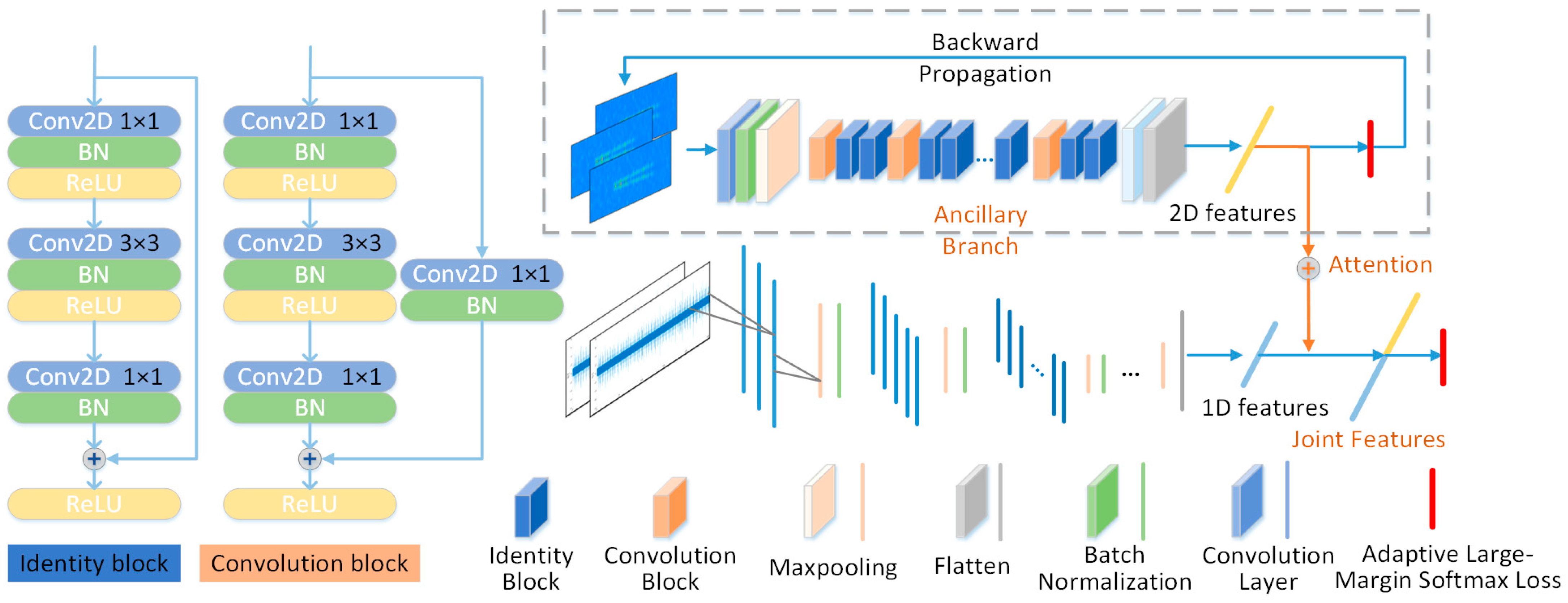
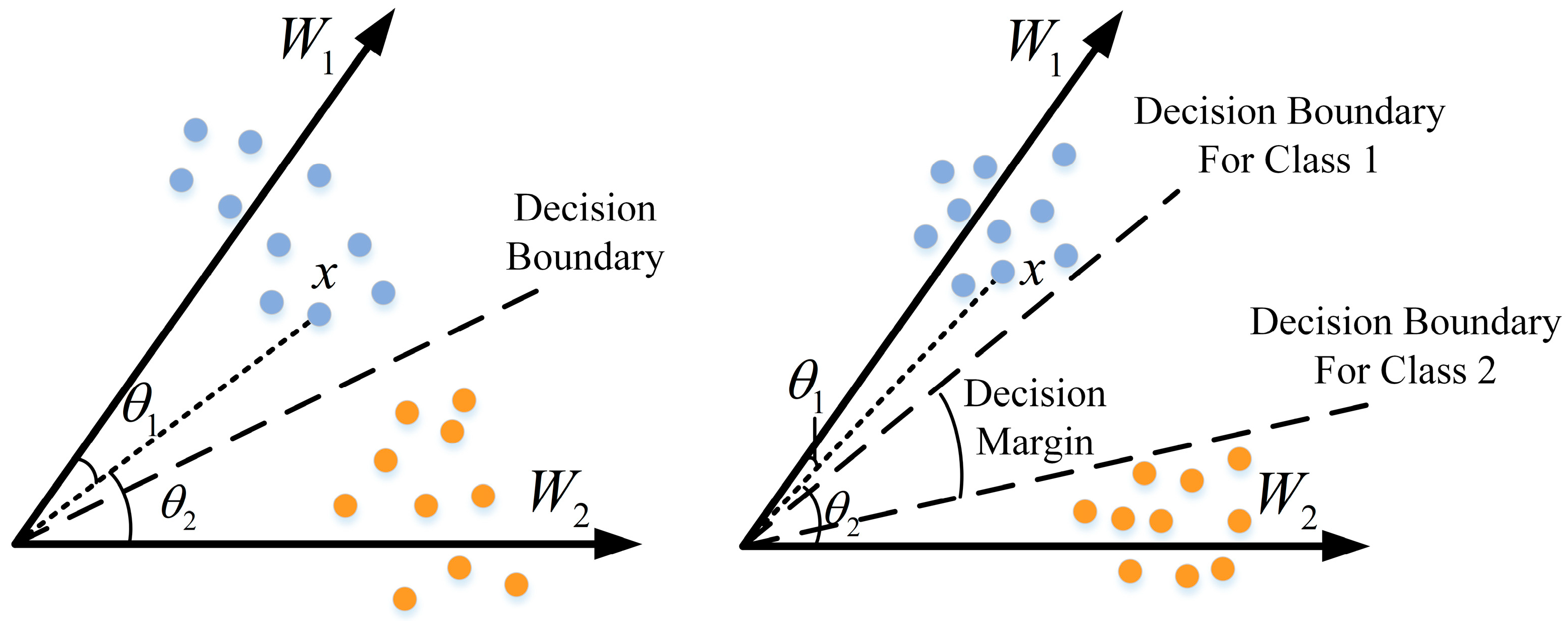
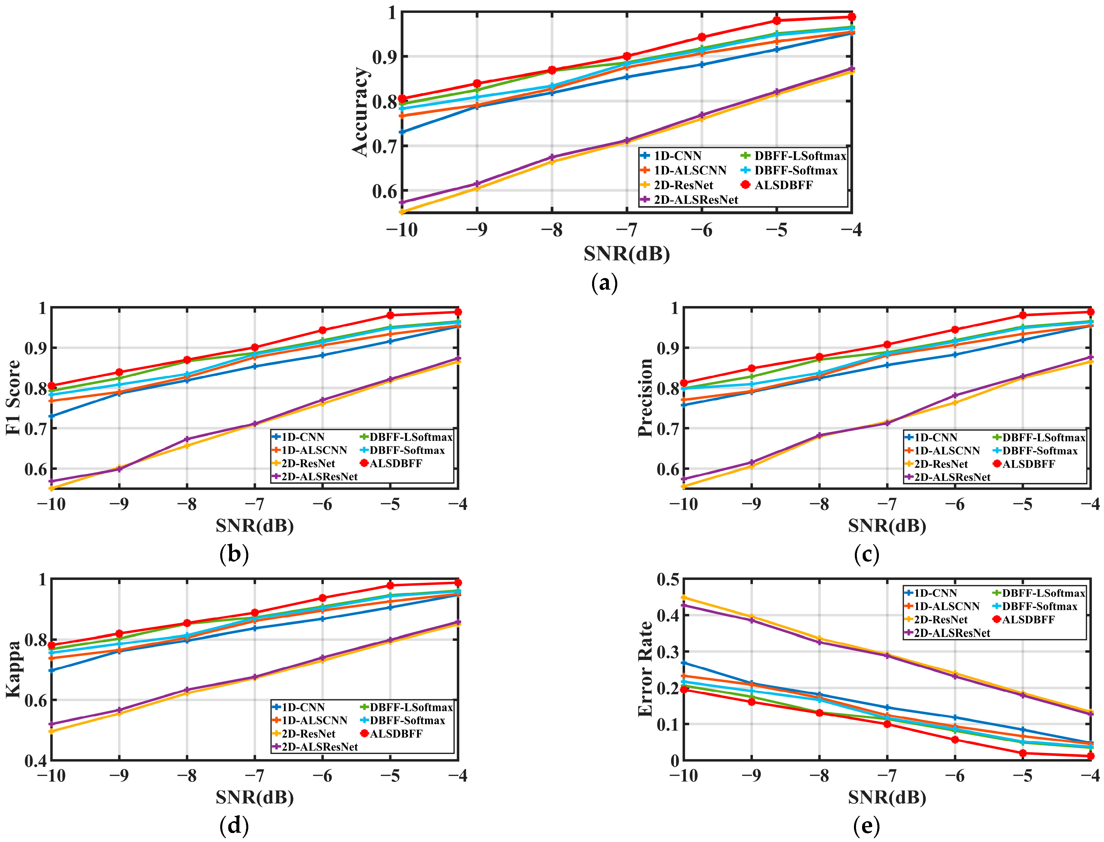
Therefore, to address the issue of low accuracy in SEI under low-SNR conditions, we have introduced an attention-enhanced dual-branch residual network that utilizes ALS. This network extracts features from one-dimensional intermediate frequency data and two-dimensional time–frequency images, fusing them with varying attention weights to form an enhanced joint feature for advanced training. This method allows for the extraction of distinctive features across dimensions, ensuring robust recognition performance amidst noise. Additionally, we replace the original Softmax with L-Softmax and further develop ALS, which adaptively calculates and adjusts the classification margin decision parameter, effectively reducing intra-class distances while increasing inter-class separations without extensive experimental tuning. Our experimental results show that this approach significantly outperforms existing methods in low-SNR scenarios, achieving an average recognition rate improvement of 4.8%.

The remainder of the paper proceeds as follows: Section 2 is concerned with the methodology used for this study. Detailed experimental procedures are given in Section 3. In Section 4, we discuss the results and analyze the factors influencing the results. Section 5 presents the conclusions derived from this study.

2. Methods

2.1. Fingerprint Feature and Time–Frequency Feature Extraction

2.1.1. Signal Envelope Fingerprint Features

The envelope feature is a significant fingerprint feature in the time domain of the radar radiation source signal and is also the most intuitive feature. It results from the physical non-idealities caused by different production batches and the processes of various hardware devices (such as power amplifiers, etc.) in radar transmitters [14], which manifest themselves in the time domain as varying degrees of envelope distortion and attenuation of the signal waveform, resulting in minor differences in the envelope of the signal pulses emitted by different radar individuals. These differences exhibit particular levels of distinctness and consistency.

The three features of envelope rising edge time [16] (rising edge slope), pulse width, and envelope top drop of different radar individuals are the least affected by environmental factors and the most reliable, and they do not fluctuate significantly with changes in the working mode and environmental factors of radar individuals. At the same time, they are less disturbed by multipath effects and other forms of interference in the transmission process, so these three features are commonly selected as fingerprint features on the envelope of radar radiation source individuals for analysis [27]. Figure 1 illustrates three different envelope fingerprint features.

2.1.2. Signal Phase Noise Fingerprint Features

In addition to the envelope fingerprint feature, the instability of the hardware system of the transmitter also affects the signal phase to some extent [28]. Specifically, some nonlinear devices’ frequency instability generated by the harmonic component and carrier cross-tuned component coupling and other nonlinear effects, as well as the resistive thermal noise in the circuit and the change in impedance caused by components such as inductors and capacitors and the noise of each resonant circuit generated by the phase parasitic modulation, can be called phase noise. In the frequency domain, it is expressed as individual differences in the frequency deviation value [29,30].

Phase noise is the phenomenon of random phase fluctuations occurring in a signal. It can be quantified by the single sideband power spectrum of phase noise, which is represented by the ratio $L(f_m)$ of power $P_{SSB}$ of the phase-modulated single sideband signal to the power $P_S$ of the carrier signal within a 1 Hz bandwidth centered at a frequency deviation $f_m$ from the carrier signal, defined as

$$L\left(f_m\right)=10\lg \left(\frac{P_{SSB}}{P_S}\right)$$

(1)

The linear frequency modulation (LFM) signal is a commonly used FM signal in radar applications and a popular method of intra-pulse phase modulation for pulse compression. Its time–frequency relationship varies linearly, and today, it is a primary transmit signal employed in most phased array radars. As a result, we simulated the phase noise of various radar systems using the LFM signal as a basis. The LFM signal is defined as

$$S\left(t\right)=A\sin \left(2\pi f_{c}t+k\pi t^2+{\varphi }_0\right),0\le t\le \tau$$

(2)

where $A$ is the amplitude, $f_c$ is the carrier frequency, $k$ is the FM slope, $\tau$ is the pulse width, and the initial phase $f_0$ is taken as 0 to simplify the analysis. The phase noise $\varphi (t)$ of the LFM signal can be approximated as a sinusoidal signal with a carrier frequency of $f_m$, expressed as

$$\varphi \left(t\right)=M\sin \left(2\pi f_{m}t\right)$$

(3)

where $M$ is the amplitude constant, also referred to as the phase modulation factor, and $f_m$ is the frequency offset. The LFM signal with phase noise can be expressed as follows:

$$S\left(t\right)=A\sin \left(2\pi f_{c}t+k\pi t^2+M\sin \left(2\pi f_{m}t\right)\right)$$

(4)

Figure 2 shows the spectrum of the LFM signal without phase noise and with three different phase noises after a short-time Fourier transform.

2.1.3. Time–Frequency Transform

Joint Time–Frequency Domain Analysis (JTFA) is a powerful tool in modern signal processing for analyzing time-varying non-stationary signals. It is also an effective method for extracting time–frequency domain features. By combining distribution information from both the time and frequency domains, this analysis method can clearly describe the relationship between signal frequency and time. Additionally, JTFA has a signal-filtering function that further enhances its utility in signal-processing applications. The short-time Fourier transform (STFT) is a widely used method in JTFA. The fundamental concept of this technique is rooted in the principles of the Fourier transform, which is a mathematical tool utilized to convert signals from the time domain to the frequency domain [31]. Specifically, for radar signals in the time domain, the Fourier transform can be expressed as follows:

$$F\left(\omega \right)=F\left[f\left(t\right)\right]={\displaystyle \underset{-\infty }{\overset{\infty }{\int }}f\left(t\right)}{e}^{-i\omega t}dt$$

(5)

where $f\left(t\right)$ is the radar signal, $F\left(\omega \right)$ is the representation of this function in the frequency domain, $e^{-i\omega t}$ is the complex exponential function, and $\omega$ is the angular frequency.

The STFT slices the time domain based on the Fourier transform. A sliding window divides the time domain signal into smaller segments. This window is centered at a specific point in time and multiplied with the radar signal to obtain its local frequency representation. If the window is small enough to ensure the signal values are smooth, the Fourier transform can be applied to each segment to obtain a time-varying frequency spectrum of the signal. This approach is commonly used in signal processing applications to analyze non-stationary signals. The STFT is defined as follows:

$$STFT\left(t,f\right)={\displaystyle \underset{-\infty }{\overset{\infty }{\int }}[z(u)g^{\ast }\left(u-t\right)]}{e}^{-2j\pi ut}du$$

(6)

where $z\left(u\right)$ is the radar signal source, and $g\left(t\right)$ is the window with a small time slice that slides along the time axis. In this study, we used the STFT to perform time–frequency transformations on radar signals, and Figure 3 shows the time–frequency diagrams of the LFM signal without individual features and with three different individual features added.

2.2. The Proposed Methods

2.2.1. Introduction to the Fundamentals of CNNs

The Convolutional Neural Network (CNN), a prime example of deep learning, was initially developed by Y. L. Cun [32]. He designed the renowned LeNet-5 for classifying handwritten digits, leveraging artificial neurons and mechanisms of visual perception. CNNs bear considerable resemblance to traditional neural networks as they both emulate the structure of human neural systems and comprise neurons with learnable weights and bias constants [32]. However, CNNs have gained wider acceptance due to their ability to bypass complex data pre-processing and directly input raw data, relying on convolution layers for feature map extraction [33].

Over the years, CNNs have evolved from their classic structure. In 2012, Geoffrey and his student Alex developed the Alex network [34], introducing a nonlinear activation function based on LeNet (ReLU) and methods to prevent overfitting (dropout, data augmentation). In 2014, K. S et al. [35] proposed VGG-Net, which incorporated more layers and utilized a uniform-size convolutional filter. The Inception structure of GoogLeNet [36] facilitated the expansion of the entire network structure in both width and depth. Residual Networks (ResNet) [37] introduced a residual learning framework to alleviate the training load on the network. This concept of residuals allows for the bypassing of the layers or segments within the network, directly forwarding the inputs to subsequent layers. This strategy effectively helps the network prevent model degradation, improving accuracy and stability.

The essence of CNNs lies in convolution, mirroring human cognition of the external world, which generally progresses from local to global. Initially, there is local perceptual awareness, which gradually expands to encompass the whole. Neurons do not need to perceive the entire image; they only need to extract local features, which is achieved by using a smaller convolution module to perform convolution operations on the input. As the convolution block slides across the entire input matrix, the local receptive fields are connected. At a higher level, the perceptions obtained from different local neurons can be integrated to acquire global information [38]. In the domain of radar signal identification, the data typically consist of 1D intermediate frequency (IF) data gathered by radar receivers and 2D time–frequency images derived from time–frequency transformations of these data. Consequently, the structure of CNNs is bifurcated into 1D-CNN and 2D-CNN, as shown in Figure 4.

2.2.2. Dual-Branch Assisted Training

In environments characterized by a low SNR, enhancing recognition accuracy solely through single-modality network training proves challenging [1,3,14]. Regardless of whether the data are a 1D sequence or transformed into a 2D time–frequency image, the signal fingerprint features are notably vulnerable to environmental noise interference. Moreover, deepening the convolutional network structure may lead to model overfitting, which contributes minimally to the enhancement of classification performance. Drawing inspiration from the human perception process, which operates from a macroscopic–local–macroscopic perspective [38,39], we propose a network structure designed for multimodal training, integrating 2D images with 1D sequences.

As depicted in Figure 5, the network is composed of two distinct branches: the 2D image auxiliary branch and the 1D sequence main branch. The auxiliary branch accepts as input an individual 2D time–frequency map, which is derived from a short-time Fourier transform. To mitigate the vanishing gradient problem that arises with increasing network depth while also allowing for flexible adjustments to the network’s depth and width to maintain its effectiveness, the architecture of ResNet alternates between “Identity Blocks” and “Convolutional Blocks”. This design enables ResNet to perform well across various tasks and datasets, whether there is a need for deeper feature learning or adjustments to the depth of feature maps to meet different output requirements [37]. The shortcut connection can be represented as follows:

$$X_L=X_l+{\displaystyle \sum _i^{L-1}F(x_i,W_i)}$$

(7)

where $X_l$ signifies the output from the preceding residual function,

$${\displaystyle \sum _{i=1}^{L-1}F(x_i,W_i)}$$

(8)

Signifies the residual function, and $X_L$ corresponds to the output of the superposition. Utilizing the chain rule, the inverse gradient can be derived as follows:

$$\frac{\partial loss}{\partial x_l}=\frac{\partial loss}{\partial x_L} · \frac{\partial x_L}{\partial x_l}=\frac{\partial loss}{\partial x_L} · \left(1+\frac{\partial }{\partial x_L}{\displaystyle \sum _{i=l}^{L-1}F(x_i,W_i)}\right)$$

(9)

The 2D feature map obtained from the auxiliary branch through the residual network is flattened and then connected with the features of the 1D sequence main branch through the weight allocation of the attention layer [40]. Since the influence of each local information in the feature map on whether the time–frequency map can be correctly identified is different, the attention mechanism can better focus on the subtle fingerprint features of the signal [41]. The formula for the attention mechanism is as follows:

$$Attention(Q,K,V)=soft\max (\frac{Q{K}^T}{\sqrt{d_k}})V$$

(10)

In the formula, Q stands for Query, K for Key, and V for Value. They are derived from the linear transformation of the input matrix X with three trainable parameter matrices, $W^Q$, $W^K$, and $W^V$, respectively. Q and $K^T$ are multiplied to generate a similarity matrix. Each element of the similarity matrix is divided by $\sqrt{d_k}$, where $d_k$ is the dimension size of K. This division is referred to as scaling. When $d_k$ is large, the variance of the product of Q and $K^T$ increases. Scaling can reduce this variance, making gradient updates more stable during training. After normalization by the Softmax function, each value has a weight coefficient greater than 0 and less than 1, and the sum of all values is 1. This result can be understood as a weight matrix. Finally, the weight matrix is multiplied by V to calculate the weighted sum, endowing the model with an attention mechanism.

The main branch is composed of 1D convolutional blocks using a pyramid structure [35]. A pyramid-structured network typically processes smaller-scale (i.e., higher-resolution) features near the input layer, which typically include low-level visual information such as edges and textures. Then, as the depth of the network increases, the scale of the processed features gradually increases, and these larger-scale features usually include parts or the whole of the object, which are higher-level visual information.

Table 1. The design scheme for the auxiliary branch network.

	Layer	Channel
auxiliary branch	Convolution Block 1	64
	Identity Block 2–3	64
	Convolution Block 4	128
	Identity Block 5–7	128
	Convolution Block 8	256
	Identity Block 9–13	256
	Convolution Block 14	512
	Identity Block 15–16	512

and

Table 2. The design scheme for the main branch network.

	Layer	Kernel Size	Channel	Max Pooling
main branch	Convolutional Layer 1–3	1 × 3	32	1 × 2
	Convolutional Layer 4–6	1 × 3	64	1 × 2
	Convolutional Layer 7–9	1 × 5	128	1 × 4
	Convolutional Layer 10–12	1 × 5	256	1 × 4

present the number of feature maps and the dimensions of the convolutional kernels for each layer. To reduce the parameter count and computational load without compromising the receptive field, we employed multiple 1 × 3 and 1 × 5 convolutional kernels as an alternative to larger ones [39]. With the network depth progression, we augmented the convolutional kernels to derive richer deep features. Subsequently, we applied max pooling to downsample the feature maps, which serves as a strategy to mitigate overfitting.

These features are combined with the image information extracted from the auxiliary branch using different attention weights to form new joint features for training. By fusing features from two dimensions, the model integrates 2D image features, which focus more on contour and location information, with 1D sequence features that change over time, thereby better distinguishing subtle differences in radar individual signals. Finally, the joint features are further learned through the improved large-margin Softmax loss function (L-Softmax) [42] to enhance the compactness within classes and separability between different radar individuals. The improved L-Softmax is one of the innovative points of this paper, and it will be detailed in the following section.

2.2.3. Adaptive L-Softmax Loss (ALS)

L-Softmax is a novel loss function proposed by Liu W, Wen Y, Yu Z et al. in 2016 [42] which improves upon the foundational Softmax loss function. The Softmax loss function is frequently used in convolutional neural networks due to its simplicity and practicality. However, it does not explicitly guide the network to learn more discriminative classification boundaries. The Softmax loss function calculates the cross-entropy loss of the results from the Softmax layer, and its formula is defined as follows:

$$L=\frac{1}{N}{\displaystyle \sum _i{L}_i}=\frac{1}{N}{\displaystyle \sum _i-\log \left(\frac{e^{f_{yi}}}{{\displaystyle \sum _j{e}^{f_j}}}\right)}$$

(11)

N represents the total number of samples, and $f_j$ represents the score of the $j$ category of sample $i$. The cross-entropy loss is calculated with the ground truth after passing through the Softmax function. Generally, $f$ is calculated by taking the dot product of the sample’s embedding feature $\varphi \left(x\right)$ and a weight vector $W$, where we denote $\varphi \left(x\right)$ as $x$. Therefore, $f_j=W_j^{T}x$. For categories 1 and 2, their weight vectors are $W_1$ and $W_2$, respectively. Therefore, for category 1, Softmax tries to learn $W_{1}x>W_{2}x$ as much as possible, that is,

$$\left|\right|W_1\left|{|}_2\right|\left|x\right|{|}_2\cos \left({\theta }_1\right)>\left|\right|W_2\left|{|}_2\right|\left|x\right|{|}_2\cos \left({\theta }_2\right)$$

(12)

${\theta }_1$ and ${\theta }_2$ are the angles between sample $x$ and $W_1$, $W_2$, respectively. For the sake of argument, let us assume that $\left|\right|W_1|{|}_2=|\left|W_2\right|{|}_2$, meaning the two weight vectors have equal lengths. At this point, Equation (12) can be simplified as:

$$\cos \left({\theta }_1\right)>\cos \left({\theta }_2\right).$$

(13)

The classification problem under this circumstance is illustrated in Figure 6.

Considering the monotonically decreasing characteristic of the cosine function in the interval [0, π], L-Softmax builds upon this by introducing a positive integer variable $m$, thereby generating a decision variable that can more strictly constrain the classification boundary. Its formula is as follows:

$$\begin{array}{l}{L}_i=-\log \left(\frac{e^{\left|\right|W_{y_i}\left|{|}_2\right|\left|x_i\right|{|}_2\psi \left({\theta }_{y_i}\right)}}{e^{\left|\right|W_{y_i}\left|{|}_2\right|\left|x_i\right|{|}_2\psi \left({\theta }_{y_i}\right)}+{\displaystyle \sum _{j\ne y_i}{e}^{\left|\right|W_j\left|{|}_2\right|\left|x_i\right|{|}_2\psi \left({\theta }_j\right)}}}\right)\\ \psi \left(\theta \right)={\left(-1\right)}^k\cos \left(m\theta \right)-2k,\\ \frac{k\pi }{m}\le \theta \le \frac{\left(k+1\right)\pi }{m},k\in \left[0,m-1\right]\end{array}.$$

(14)

The L-Softmax loss has a clear geometric interpretation, as shown in Figure 6 The variable $m$ controls the gap between categories. As $m$ increases, the margin between classes becomes larger, making the learning more challenging, which can effectively prevent overfitting [43].

The introduction of L-Softmax has significantly increased the margin between decision boundaries of similar classes. However, its approach of directly multiplying by a fixed $m$ to forcibly increase the angular margin between classes for enhanced discriminative power of the model is a simple linear method. This method requires adjusting the size of parameter $m$ to achieve optimal classification results when facing different problems. Therefore, to make the adjustment of the angular margin more flexible, we propose ALS based on L-Softmax. This allows the model to adaptively adjust the size of parameter $m$ according to the magnitude of the classification boundaries. In this approach, $m$ is no longer a fixed parameter that needs to be set based on experimental results; instead, it is replaced with an adaptive parameter $m^{\prime }$, whose calculation formula is as follows:

$$m^{\prime }=\frac{\pi +c}{\theta +c}.$$

(15)

In the formula, to avoid the denominator approaching 0 when θ is close to 0, a constant $c$ is added to both the numerator and the denominator. Furthermore, $c$ can also control the range of values for $m^{\prime }$. To maintain consistency with ref. [42], where $m=2,3,4$, we set $c=\frac{\pi }{3}$ in this study. Consequently, when $\theta$ is within [0, π], $m^{\prime }$ falls within the range [1,4]. The range of variation for $m^{\prime }$ can be adjusted for different task requirements by calculating $c$. Based on the derivation of the above formula, it becomes evident that when $\theta$ is small, indicating that the classification margin is small and the categories are close to each other, $m^{\prime }$ obtains a larger value close to 4, which amplifies the angular difference, which helps to increase the inter-class distance. As $\theta$ increases, indicating a large margin between classes and making them easier to distinguish, the value of $m^{\prime }$ decreases. When $\theta =\pi$, it can be derived that $m^{\prime }=1$. Under this condition, the ALS method degenerates into the Softmax. This approach avoids excessive amplification for larger values of $m^{\prime }$, thereby maintaining the reasonableness of the inter-class distance to a certain extent.

3. Experiments and Results

We simulated multiple datasets of pulse signals originating from different radar emitters at different SNRs. These datasets were utilized for training and testing the proposed method and other baseline methods in terms of their capabilities in SEI. The experiments described in this article were based on the basic framework of Tensorflow and Keras to construct neural networks with an Intel 10900K CPU, Santa Clara, CA, USA, with 128GB of RAM and an RTX 3090 GPU.

3.1. Dataset and Parameter Setting

Typically, conventional radar signals are characterized by high-power radio frequency pulses, with a carrier band spanning from 3 MHz to 100 GHz. In our simulation, the radar receiver employed a local oscillator (LO) to mix with the high-frequency radar signal, thereby down-converting the frequency of the received signal. This process yields a lower-frequency signal via the intermediate frequency (IF) amplifier. More specifically, a mixer was employed in the simulation to down-convert the frequency of the received signal, thereby ensuring a precise representation of the radar system’s operation within a real-world environment. This mixer operates by multiplying the RF signal with the local oscillator signal, resulting in two output frequencies: the sum and the difference between the radio frequency $f_{RF}$ and the LO frequency $f_{LO}$, which can be represented as follows:

$$f_{RF}+f_{LO}$$

(16)

$$f_{RF}-f_{LO}$$

(17)

Obviously, for the convenience of subsequent signal processing, we need to obtain the lower frequencies $f_{RF}-f_{LO}$, which serve as the intermediate frequency (IF). By using a low-pass filter, we can effectively suppress the summed frequencies $f_{RF}+f_{LO}$, thereby isolating the subtracted frequencies that constitute the IF signal. According to the Nyquist sampling theorem, the sampling frequency of a signal should be at least twice the bandwidth of it. In most cases, the modulation bandwidth of radar signals is less than the instantaneous receiving bandwidth of radar reconnaissance equipment, the latter typically ranging from tens of megahertz to gigahertz. Therefore, in our experiment, we have chosen a sampling frequency of 1 GHz.

In order to simulate the nonlinear variations in transmitted signals caused by physical hardware as accurately as possible, we referenced the characteristics of signals received by radar receivers in reality and several validated research articles from various dimensions, such as the time domain and frequency domain [14,26,27,28,29,30,31]. In our simulation, we first modeled three different radar systems by adjusting parameters such as pulse width (PW), bandwidth (BW), and radio frequency (RF), also known as the carrier frequency. Based on these models, we then simulated three unique transmitters for each model by varying key fingerprint features such as the radio frequency offset (RFO), phase-noise frequency offset (PNFO), and phase modulation coefficient (PMC) [10]. Additionally, we adjusted envelope attributes such as the filter sample frequency (FSF) and the filter cutoff frequency (FCF). This process allowed us to generate nine individual distinct radar emitter signals. Details of the parameters of the simulated signals used in the experiments of this study are shown in

Table 3. Parameter configuration of radar individual signal fingerprint features.

Type		PW/μs	BW/MHz	RFO/MHz	PNFO/Hz	PMC	FSF/MHz	FCF/Hz
1	1	1.5 ± 0.3	40	2.0 × 10–4	[1.0 K 10 K 100 K 1.0 M 10 M]	[1.0 0.1 0.01 0.001 0.0001]	20	200
	2	1.5 ± 0.3	40	1.5 × 10–4	[10 K 80 K 3 M 18 M 70 M]	[0.5 0.1 0.03 0.007 0.0004]	30	150
	3	1.5 ± 0.3	40	2.5 × 10–4	[5 K 30 K 400 K 7 M 50 M]	[0.8 0.2 0.04 0.003 0.0006]	30	200
2	1	2.0 ± 0.3	30	2.1 × 10–4	[1.1 K 11 K 101 K 1.1 M 11 M]	[1.1 0.2 0.02 0.002 0.0002]	20	200
	2	2.0 ± 0.3	30	1.6 × 10–4	[12 K 60 K 4 M 20 M 80 M]	[0.3 0.1 0.02 0.006 0.0003]	30	150
	3	2.0 ± 0.3	30	2.6 × 10–4	[8 K 20 K 100 K 8 M 60 M]	[0.9 0.3 0.05 0.004 0.0006]	30	200
3	1	2.5 ± 0.3	20	2.2 × 10–4	[1.2 K 12 K 101 K 1.2 M 12 M]	[1.2 0.3 0.03 0.003 0.0003]	20	200
	2	2.5 ± 0.3	20	1.7 × 10–4	[15 K 70 K 5 M 22 M 60 M]	[0.4 0.1 0.01 0.005 0.0002]	30	150
	3	2.5 ± 0.3	20	2.7 × 10–4	[7 K 20 K 200 K 9 M 70 M]	[0.6 0.4 0.03 0.002 0.0004]	30	200

.

We introduced simulated additive noise into all signals to emulate a realistic electromagnetic environment. In radar signal processing, additive Gaussian white noise (AWGN) is the most common noise. This noise simulates the natural random variations that occur during the signal transmission process, with its power spectral density being uniform across the entire frequency range. In addition, the signal may also be affected by Rayleigh noise due to multipath effects, and due to errors in the radar system, the signal may contain uniformly distributed noise. Figure 7 shows the superposition of different noises with the signal for simulation.

AWGN is prevalent in many natural and artificial systems. In nature, the outcomes of many random processes tend to follow a Gaussian distribution. According to the Central Limit Theorem, the sum of multiple independent random variables approximates a Gaussian distribution, even if these variables do not follow a Gaussian distribution. In technical systems such as electronic devices, the noise generated by the superposition of various factors, including resistance, current, and thermal effects, also tends to approximate a Gaussian distribution. Therefore, due to the ubiquity of Gaussian white noise in both natural and technical systems, its favorable statistical properties, and its convenience, these properties ensure that the specific waveform characteristics of the noise do not have a significant impact on the method’s performance. In this study, we chose to superimpose Gaussian white noise with the simulation signal. The model representing the radar signal intercepted by the receiver is as follows:

$$x(t)=s(t)+n(t)$$

(18)

$n(t)$ is white Gaussian noise, and $s(t)$ is the radar signal. The SNR is defined as:

$$SNR=10{\log }_{10}\frac{P_S}{P_N}$$

(19)

To assess the algorithm’s recognition capabilities under various low-SNR scenarios, we configured multiple low-SNR environments for the nine distinct radar transmitter signal datasets outlined in the preceding table. Each dataset was synthesized under identical SNR conditions, with SNRs extending from −10 dB to −4 dB at 1 dB intervals. For these training sets, we proportionally allocated the data into training, validation, and test sets at a ratio of 4:1:1. For example, with a training set comprising 4500 samples at each SNR level (encompassing 7 SNR levels from −10 to −4 dB), the corresponding validation and test sets would each contain 1125 samples. Figure 8 illustrates the temporal waveforms of the nine individual radar signals listed in Table 3 at an SNR of −4 dB.

3.2. Experiments on the Proposed Method

In this section, we present the use of the nine distinct radar emitter IF signal datasets described in Section 3.1 as the input for the 1D sequence main branch of the dual-branch network and the 2D time–frequency images produced through the time–frequency transformation presented in Section 2.1.3 as the network input for the 2D image auxiliary branch.

Both branches utilize the cross-entropy loss function and the Adam optimizer, with a 0.0001 learning rate and 32 batch size. Each branch extracts features from data of different dimensions. The auxiliary branch, which extracts 2D time–frequency features, assigns varying weights through an attention layer after the flattening layer to fuse with the 1D features from the main branch. Subsequently, the ALS (mentioned in Section 2.2.3) enhances the disparity of features between individual radar signal categories, preventing network overfitting. The network weights were saved when the highest accuracy was achieved on the validation set. The specific experimental procedure is as follows:

• Initialize the network parameters, training and optimizing both the 1D intermediate frequency (IF) sequence and the 2D time–frequency image branches simultaneously in a dual-input, dual-output format;
• Flatten the feature maps extracted by the last identity convolution block of the 2D image auxiliary branch, calculate and assign attention weights through the attention layer, and form a joint feature vector with the flattened features from the 1D IF sequence main branch;
• Apply the ALS to the joint feature vector, introducing adaptive decision variables to constrain the classification boundaries, reducing the feature distance within the same category of radar individual signals and increasing the disparity between categories. Then, compute the loss of the joint feature vector;
• The loss of the joint features serves as the overall loss for both branches, which is backpropagated to each branch for the optimization and updating of network parameters;
• Save the network weights when the highest accuracy on the validation set is achieved, independently conduct each experiment and repeat each one 10 times, and take the average of multiple experiments as the final test result.

Based on the experimental procedure described above, we documented and preserved the variation in validation set accuracy concerning the number of training epochs, as shown in Figure 9.

As depicted in Figure 9, the model’s accuracy on the validation set fluctuates significantly in the early stages of training (first 100 epochs). As the training iterations progress, the model’s accuracy on the validation dataset tends to stabilize. It is worth noting that after the 200th training iteration, the accuracy reaches an almost constant state, indicating that the model has converged. We store the weights corresponding to the highest accuracy on the validation set during the training process for subsequent testing.

To further assess the classification performance of the multi-class network, we introduced additional metrics beyond accuracy and loss, including precision, error rate, F1 score, and Kappa [44]. Accuracy is the proportion of correctly predicted observations to the total observations. It reflects the overall effectiveness of a model in classifying instances correctly. However, it may not be a reliable indicator on its own, especially in cases where class distributions are imbalanced. The error rate is the proportion of incorrectly predicted observations to the total observations. Precision for a specific class is the number of true positives (correctly predicted instances of the class) divided by the total number of samples predicted to belong to that class (the sum of true positives and false positives). The F1 Score is the harmonic mean of precision and recall. The F1 score conveys the balance between precision and recall, which is particularly useful when the class distribution is uneven. Cohen’s Kappa, commonly referred to as Kappa, quantifies the concordance between predicted and true classifications, adjusting for the likelihood of random agreement. This metric offers a refined perspective on the model’s predictive performance. Consequently, we have obtained the network classification performance scores on the test set of the proposed method ALSDBFF under various SNRs, as presented in

Table 4. The network classification performance metrics for radar individual signals, based on ALSDBFF across various SNRs.

SNR/dB	Accuracy	Error Rate	Precision	F1 Score	Kappa
−10	0.8053	0.1947	0.8124	0.8055	0.781
−9	0.8391	0.1609	0.8489	0.8394	0.819
−8	0.8693	0.1307	0.8772	0.8698	0.853
−7	0.9102	0.0897	0.9135	0.9102	0.899
−6	0.9431	0.0569	0.9448	0.9432	0.936
−5	0.9804	0.0196	0.9807	0.9805	0.978
−4	0.9884	0.0116	0.9886	0.9885	0.987

.

As shown in Table 4, the conclusion can be drawn that the proposed method performs well under various low-SNR conditions, with the average classification accuracy steadily increasing as the SNR improves. When the SNR is greater than or equal to −7 dB, the classification accuracy of the test set consistently exceeds 90%. Furthermore, the model achieves high scores in metrics such as Precision, F1 Score, and Kappa, indicating that the model does not learn from class imbalance in this multi-classification task and maintains good consistency and classification performance.

3.3. Comparisons with Other Baseline Methods

To demonstrate the effectiveness of the dual-branch fusion and our proposed Adaptive L-Softmax Loss (ALS), we constructed seven models based on different network structures or the addition of these enhancements while ensuring they all share the same convolutional layers, kernel sizes, fully connected layers, batch normalization layers, etc. We used 1D-CNN [45] and 2D-ResNet50 [46] as the baseline control groups and then named the 1D-CNN with the added ALS function as 1D-ALSCNN and the 2D-ResNet50 with the added ALS function as 2D-ALSResNet50. The dual-branch feature fusion of 1D-CNN and 2D-ResNet50, which does not incorporate the ALS enhancement, is named the DBFF-Softmax and employs the standard Softmax, while the network using L-Softmax is named DBFF-LSoftmax. The model proposed in this paper, based on ALS, is named ALSDBFF, as shown in

Table 5. Differences between the proposed method and other baseline methods.

	Feature Fusion	L-Softmax	Attention L-Softmax
1D-CNN	no	no	no
2D-ResNet50	no	no	no
1D-ALSCNN	no	no	yes
2D-ALSResNet50	no	no	yes
DBFF-Softmax	yes	no	no
DBFF-LSoftmax	yes	yes	no
ALSDBFF	yes	yes	yes

“yes” means that the model uses this improvement; “no” means it is not used.

.

In

Table 6. The classification accuracy of different methods at different SNRs.

Methods	−10	−9	−8	−7	−6	−5	−4	AA
1D-CNN	0.7307	0.7876	0.8187	0.8542	0.8818	0.9156	0.9521	0.8486
2D-ResNet50	0.5520	0.6044	0.6641	0.7084	0.7601	0.8151	0.8658	0.7099
1D-ALSCNN	0.7671	0.7911	0.8276	0.8756	0.9067	0.9333	0.9547	0.8651
2D-ALSResNet50	0.5733	0.6151	0.6747	0.7121	0.7689	0.8213	0.8729	0.7197
DBFF-Softmax	0.7831	0.8089	0.8338	0.8836	0.9138	0.9484	0.9627	0.8763
DBFF-LSoftmax	0.7938	0.8249	0.8676	0.8862	0.9182	0.9511	0.9653	0.8867
ALSDBFF	0.8053	0.8391	0.8693	0.9102	0.9431	0.9804	0.9884	0.9051

, we compare the classification accuracy of the method proposed in this paper (ALSDBFF) with other baseline methods under different SNR conditions and calculate their average accuracy (AA). To more clearly observe the classification accuracy of different methods for each radar individual signal category, we have plotted the confusion matrices of these methods under the -4dB condition, as shown in Figure 10.

As shown in Table 6 and Figure 10, the recognition effects of the two baseline methods, the 1D-CNN using only the IF sequence (Figure 10b) and the 2D-ResNet50 using only the time–frequency images (Figure 10c), are the poorest, especially for the 2D-ResNet50 network, which experienced confusion in most categories, with the highest misclassification in categories 1, 3, 6, and 9. This is due to the subtle features in the images being easily disturbed by noise, particularly evident in low-noise situations, presenting a challenge for the 2D-ResNet50 method. Incorporating our proposed ALS method into the 1D-CNN and 2D-ResNet50 (as shown in Figure 10e,f) can effectively enhance network recognition performance and reduce the number of misclassified samples. Furthermore, the network that trains and recognizes using joint features formed by fusing one-dimensional features with two-dimensional time–frequency features, DBFF-Softmax (as shown in Figure 10d), significantly reduces the impact of noise. The recognition effect is superior to that of using the single features of 1D-CNN and 2D-ResNet50 alone, indicating that the dual-branch feature fusion network structure helps improve network stability. DBFF-LSoftmax (as shown in Figure 10g), which improves upon Softmax, further enhances the recognition rate. Our proposed method (ALSDBFF, as shown in Figure 10a), which utilizes both the DBFF network structure and the ALS method, greatly ameliorates the misclassification issues in categories 1, 3, 6, and 9 and enhances the recognition accuracy of individual radar signals under different low-SNR conditions, achieving an average recognition rate of 90.51%. Even under the condition of −10 dB, the recognition accuracy of our proposed algorithm exceeds 80%. Meanwhile, the model’s recognition capability steadily improved as the SNR increased.

As illustrated in Figure 11, we also evaluated seven networks using metrics such as Error Rate, Precision, F1 Score, and Kappa, and based on these, we plotted performance line charts under various SNRs. From the figure, we can draw the same conclusion that the method we proposed has enhanced the stability and accuracy of the network, achieving superior performance across different scenarios.

4. Discussion

4.1. Effect of Different Number of Layers in the Auxiliary Branch ResNet Network on Experimental Results

In Section 2.2.2, we described our employment of the standard ResNet50 network structure as the auxiliary branch within the dual-branch network architecture. This choice is attributed to the ResNet network’s capability to preserve original features through residual connections while training deeper neural networks, thereby enhancing the network’s ability to learn and represent features of two-dimensional images. The classic and widely used ResNet variants include ResNet18, ResNet34, ResNet50, and ResNet101. Therefore, when constructing the layer structure of the auxiliary branch ResNet network, we conducted experimental comparisons with various ResNet networks under different SNR conditions to select the optimal network structure.

Table 7. Classification accuracy of different layers of ResNet within auxiliary branch at different SNRs.

Auxiliary Branch ResNet Network	−10	−9	−8	−7	−6	−5	−4	AA
ResNet-18	0.6844	0.7813	0.8462	0.9004	0.9402	0.9698	0.9716	0.8706
ResNet-34	0.7973	0.8322	0.8658	0.8978	0.9227	0.9662	0.9707	0.8932
ResNet-50	0.8053	0.8391	0.8693	0.9102	0.9431	0.9804	0.9884	0.9051
ResNet-101	0.8108	0.8311	0.8649	0.9076	0.9438	0.9609	0.9796	0.8998

was generated using the average classification accuracy as the metric.

As shown in Table 7, with the increase in the number of layers in the ResNet network from 18 to 34 and then to 50, the ability of the auxiliary branch to extract features and learn deep image information gradually strengthens, resulting in a significant improvement in the accuracy of recognition. However, this does not mean that the deeper the network, the better. When we increased the number of ResNet layers from 50 to 101, it was observed that the recognition accuracy of the ResNet-101 network did not improve as expected. Instead, there was a decrease in recognition rates in more than half of the datasets, with only a slight advantage in the −10 dB and −6 dB datasets. Based on analysis, we believe that the excessive depth of the network may have caused overfitting or slow optimization due to the massive number of network parameters. Moreover, with the same set of hyperparameters, the training time per epoch for ResNet-101 is 25 s, 225 ms/step, compared to 16s, 144 ms/step for ResNet-50. The training time cost far exceeds that of ResNet-50. Therefore, we ultimately selected the classic structure of ResNet-50 as the auxiliary branch.

4.2. The Number of Iterations and Time per Iteration for Training the Model via Different Methods

From the experiments described in Section 3, it can be concluded that our method performs well under various SNR conditions. However, evaluating the merits of a network also requires a comprehensive consideration of the time cost incurred during its training process, as well as the network’s convergence speed. These factors are crucial in determining the suitable application scenarios and resource conditions for different networks. Therefore, we compared the time cost of training different networks under the same experimental conditions on the same dataset (taking −4 dB as an example), as shown in

Table 8. The number of iterations and time per iteration for training the model via different methods.

	Number of Epochs	Time per Epoch (RTX3090)
1D-CNN	122	2 s
2D-ResNet50	153	15 s
1D-ALSCNN	144	2 s
2D-ALSResNet50	180	15 s
DBFF-Softmax	161	18 s
DBFF-LSoftmax	189	19 s
ALSDBFF	167	18 s

.

During the experimental process, we employed an early stopping strategy for training: If the model’s performance does not show significant improvement on the validation set over ten consecutive training epochs, the model may begin to overfit the training data. At this point, the training process will be prematurely terminated to prevent overfitting and to save training time when there is no further improvement in model performance. To better observe the training time, we have presented the results in a bar chart (shown in Figure 12).

From Table 8 and Figure 12, we can conclude that the three methods utilizing a dual-branch network structure (DBFF-Softmax, DBFF-LSoftmax, and the proposed method) require simultaneous training on one-dimensional data and two-dimensional images, resulting in longer training times per epoch compared to models which only use a single branch or a single dimension. Furthermore, the L-Softmax loss function further increases the complexity of network optimization, necessitating more epochs for the model to converge. Therefore, although the method proposed in this paper significantly improves network recognition performance compared to other methods, it has issues such as its longer training times and slower model convergence rates, making it unsuitable for scenarios that require shorter training periods. In our future work, we will focus on model optimization and improving training speed.

4.3. Impact of the Sampling Rate on the Performance of the Method

In our aforementioned experiment, the signal sampling frequency was fixed and set at 1 GHz. These settings of the sampling frequency, along with the signal bandwidth and pulse width, primarily affect the length of the simulated one-dimensional signal. Specifically, the sampling frequency determines the number of samples per unit time, the bandwidth affects the frequency range of the signal, and the pulse width influences the sampling duration of the signal. These factors, together, lead to variations in signal length and the degree of similarity between signals of different classes within the dataset. In Section 3.1, we described how we adjusted the degree of similarity between the types of signals by changing the pulse width and bandwidth, generating nine different types of radar individual signals. Therefore, in this section, we mainly discuss the impact of the sampling rate on our method and enrich and supplement the original dataset accordingly.

According to the Nyquist low-pass sampling theorem, the sampling frequency must be at least twice the signal bandwidth. However, to ensure that the subtle individual characteristics of the signal are as detailedly described and preserved as much as possible during the sampling process, we adjusted the sampling rates to three levels: low, medium, and high, which are 500 MHz, 1 GHz, and 2 GHz, respectively. We validated the generalization performance of this method under different sampling rates using the −5 dB dataset as a representative, as shown in

Table 9. Classification performance for proposed method based on different sampling rates.

Sampling Rates	Accuracy	Error Rate	Precision	F1 Score	Kappa
500 MHz	0.9753	0.0247	0.9786	0.9758	0.971
1 MHz	0.9804	0.0196	0.9807	0.9805	0.978
2 MHz	0.9863	0.0137	0.9872	0.9871	0.982

.

We concluded that, with other parameters remaining constant, changing the sampling rate, which alters the data length, indeed impacts the network’s recognition performance, but the overall effect is minimal. This demonstrates that the method we proposed exhibits a certain degree of robustness on datasets of varying lengths.

5. Conclusions

To address the problem of the poor classification accuracy of radar individual signal characteristics within low-SNR conditions, where the single-dimensional radar individual signal features are severely affected by noise, we propose the ALSDBFF for radar individual signal classification. We designed a dual-branch network structure to extract features from one-dimensional IF data and two-dimensional time–frequency images and assign the weights of the features, fusing them into an enhanced joint feature for continued training. Additionally, we introduced the Adaptive L-Softmax method (ALS) to replace the original Softmax, which adaptively calculates the classification margin decision parameter based on the angle between samples and the classification boundary and adjusts the margin values of the sample classification boundaries; it reduces the intra-class distance for the same class while increasing the inter-class distance between different classes without the need for cumbersome experiments to determine the optimal value of decision parameter.

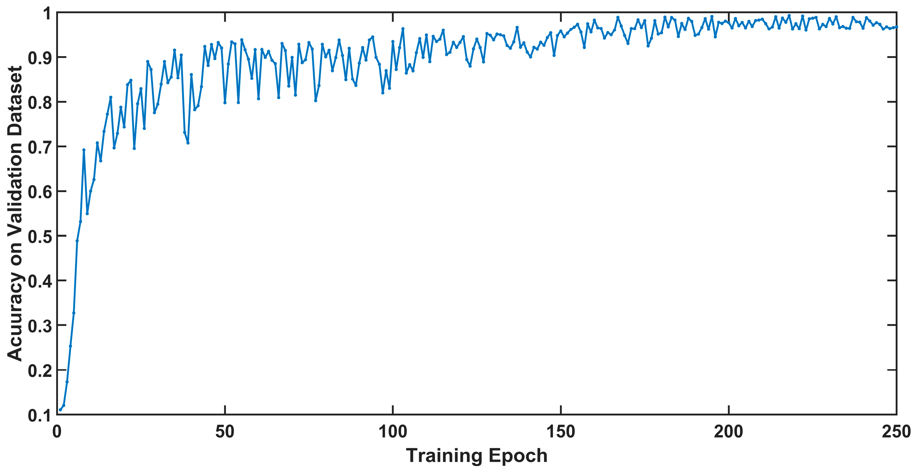
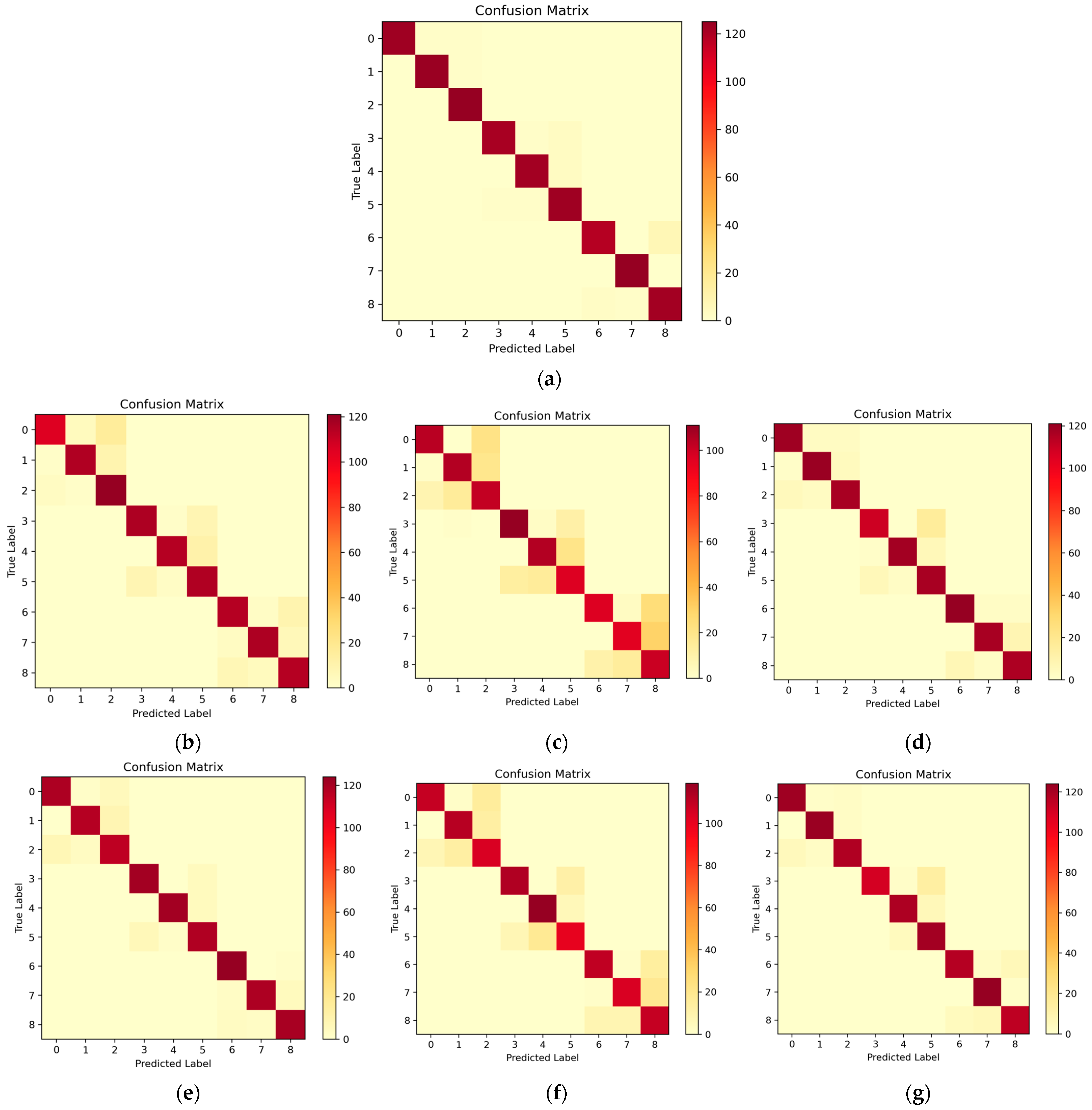
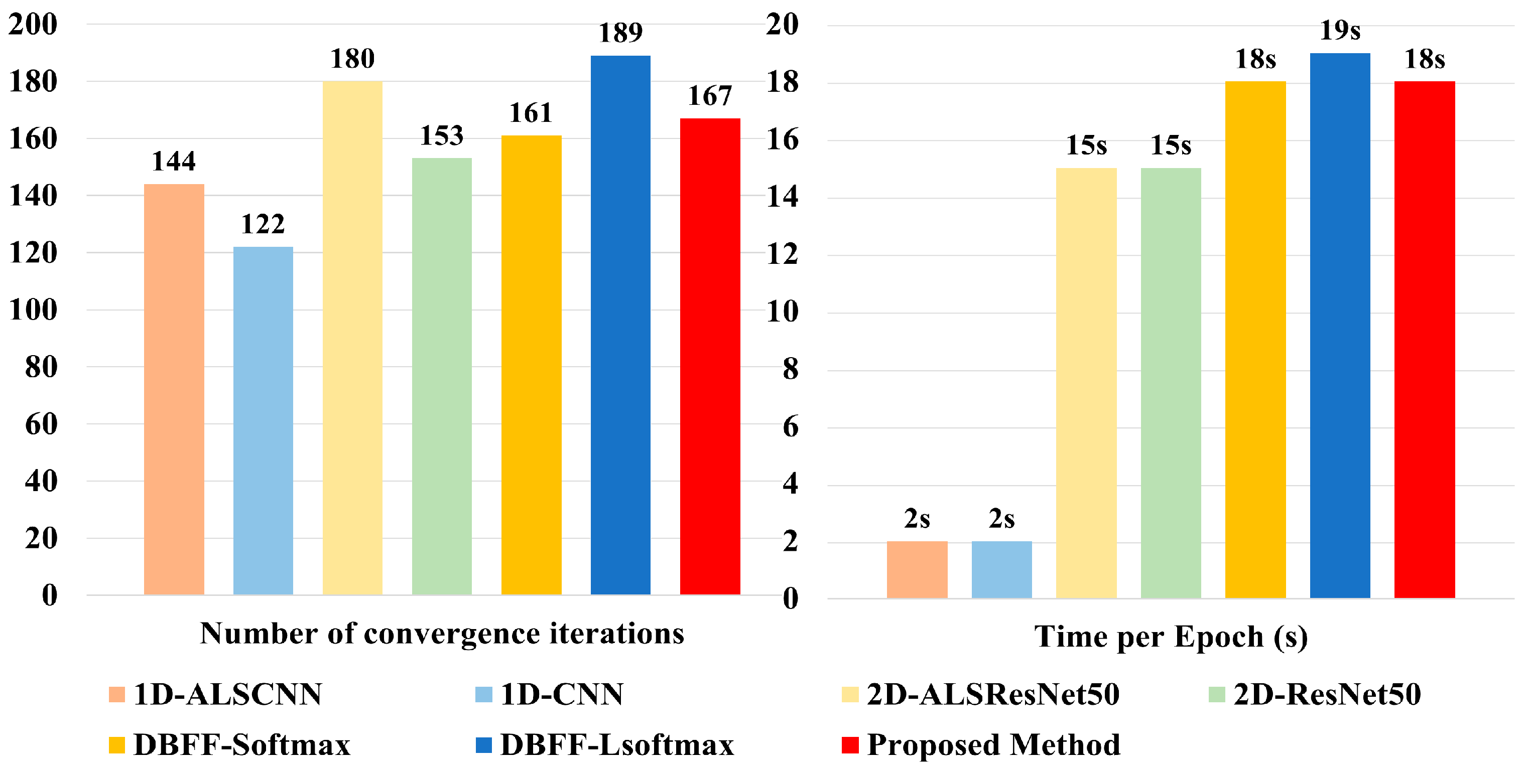
The experimental results demonstrate that relative to other baseline approaches, the proposed method significantly improves the model’s ability to extract features and classify data under low-SNR conditions, effectively mitigating the influence of noise. Compared to models using only single-dimensional features (1D-CNN, 2D-ResNet), the network structure utilizing dual-branch feature fusion achieves an average classification accuracy rate improvement of 9.7%. Further experimental investigation into the effects of ALS indicates that employing L-Softmax aids the model in enlarging the distance between different classes, thus diminishing the likelihood of misclassification among similar categories. Compared to Softmax, the average classification accuracy rate improved by 1.04%, and the accuracy rate was further enhanced by 1.84% when using the attention mechanism with L-Softmax compared to L-Softmax alone. However, we also recognize the shortcomings of our method. Firstly, although the dual-branch network structure improves the network’s classification accuracy rate and stability, it somewhat sacrifices training speed. Meanwhile, the L-Softmax makes the model more difficult to converge during training, requiring a greater time investment. Secondly, the auxiliary branch’s ResNet network structure is prone to overfitting, posing challenges in enhancing the model’s validation set accuracy throughout the training process.

In future work, we hope to continue improving this method, enhancing network training efficiency, reducing training time costs, and reducing overfitting through designing or improving loss function methods. Meanwhile, we plan to collect real-world data to further refine our model to ensure its robustness and reliability in real-world applications.

References

1. Yu, S.; Zheng, Y.; Wang, J.; Huang, J. A new method for radar emitter individual identification based on VMD and multi-image feature combination. In Proceedings of the 7th International Conference on Vision, Image and Signal Processing (ICVISP), Dali, China, 24–26 November 2023. [Google Scholar]
2. Liu, C.; Fu, X.; Wang, Y.; Guo, L.; Liu, Y.; Lin, Y.; Zhao, H.; Gui, G. Overcoming Data Limitations: A Few-Shot Specific Emitter Identification Method Using Self-Supervised Learning and Adversarial Augmentation. IEEE Trans. Inf. Forensics Secur. 2024, 19, 500–513. [Google Scholar] [CrossRef]
3. Zhu, Z.; Ji, H.; Li, L. Deep Multimodal Subspace Interactive Mutual Network for Specific Emitter Identification. IEEE Trans. Aerosp. Electron. Syst. 2023, 59, 4289–4300. [Google Scholar] [CrossRef]
4. He, B.; Wang, F. Specific Emitter Identification via Sparse Bayesian Learning Versus Model-Agnostic Meta-Learning. IEEE Trans. Inf. Forensics Secur. 2023, 18, 3677–3691. [Google Scholar] [CrossRef]
5. Liao, Y.; Li, H.; Cao, Y.; Liu, Z.; Wang, W.; Liu, X. Fast Fourier Transform with Multihead Attention for Specific Emitter Identification. IEEE Trans. Instrum. Meas. 2024, 73, 2503812. [Google Scholar] [CrossRef]
6. Hua, M.; Zhang, Y.; Sun, J.; Adebisi, B.; Ohtsuki, T.; Gui, G.; Wu, H.-C.; Sari, H. Specific Emitter Identification Using Adaptive Signal Feature Embedded Knowledge Graph. IEEE Internet Things J. 2024, 11, 4722–4734. [Google Scholar] [CrossRef]
7. Liu, Z.; Gao, H.; Chen, J.; Zhou, D.; Li, Y.; Sun, S.; Xiang, R. Individual Intelligent Recognition Method Based on Fingerprint Features of Radar Emitter. In Proceedings of the 2021 CIE International Conference on Radar (Radar), Haikou, China, 15–19 December 2021; pp. 2137–2141. [Google Scholar]
8. Han, X.; Chen, S.; Chen, M.; Yang, J. Radar specific emitter identification based on open-selective kernel residual network. Digit. Signal Process. 2023, 134, 103913. [Google Scholar] [CrossRef]
9. Liu, M.; Doherty, J. Nonlinearity estimation for specific emitter identification in multipath channels. IEEE Trans. Inf. Forensics Secur. 2011, 6, 1076–1085. [Google Scholar]
10. Liu, S.; Yan, X.; Li, P.; Hao, X.; Wang, K. Radar emitter recognition based on SIFT position and scale features. IEEE Trans. Circuits Syst. II Express Briefs 2018, 65, 2062–2066. [Google Scholar] [CrossRef]
11. Guo, S.; Xu, Y.; Huang, W.; Liu, B. Specific Emitter Identification via Variational Mode Decomposition and Histogram of Oriented Gradient. In Proceedings of the 2021 28th International Conference on Telecommunications (ICT), London, UK, 1–3 June 2021; pp. 1–6. [Google Scholar]
12. Xue, J.; Tang, L.; Zhang, X.; Jin, L. A Novel Method of Radar Emitter Identification Based on the Coherent Feature. Appl. Sci. 2020, 10, 5256. [Google Scholar] [CrossRef]
13. Zhou, Z.; Huang, G.; Chen, H.; Gao, J. An overview of radar emitter recognition algorithms. Telecommun. Eng. 2017, 57, 973–980. [Google Scholar]
14. Zhong, Y.; Zhang, L.; Pu, W. Multimodal Deep Learning Model for Specific Emitter Identification. In Proceedings of the 2021 IEEE 6th International Conference on Signal and Image Processing (ICSIP), Nanjing, China, 22–24 October 2021; pp. 857–860. [Google Scholar]
15. Li, L.; Ji, H. Specific emitter identification based on ambiguity function. J. Electron. Inf. Technol. 2009, 31, 2546–2551. [Google Scholar]
16. Ru, X.; Ye, H.; Liu, Z.; Huang, Z.; Wang, F.; Jiang, W. An experimental study on secondary radar transponder UMOP characteristics. In Proceedings of the 2016 European Radar Conference (EuRAD), London, UK, 5–7 October 2016; pp. 314–317. [Google Scholar]
17. Carroll, T.L. A nonlinear dynamics method for signal identification. Chaos 2007, 17, 023109. [Google Scholar] [CrossRef] [PubMed]
18. Xu, D.; Yang, B.; Jiang, W.; Zhou, Y. An improved SVDU-IKPCA algorithm for Specific Emitter Identification. In Proceedings of the 2008 International Conference on Information and Automation, Changsha, China, 20–23 June 2008; pp. 692–696. [Google Scholar]
19. Ding, L.; Wang, S.; Wang, F.; Zhang, W. Specific Emitter Identification via Convolutional Neural Networks. IEEE Commun. Lett. 2018, 22, 2591–2594. [Google Scholar] [CrossRef]
20. Chen, T.; Jin, W.; Li, J. Feature extraction using surrounding-line integral bispectrum for radar emitter signal. In Proceedings of the 2008 IEEE International Joint Conference on Neural Networks (IEEE World Congress on Computational Intelligence), Hong Kong, China, 1–8 June 2008; pp. 294–298. [Google Scholar]
21. Wang, L.; Ji, H.; Shi, Y. Feature extraction and optimization of representative-slice in ambiguity function for moving radar emitter recognition. In Proceedings of the 2010 IEEE International Conference on Acoustics Speech and Signal Processing (ICASSP), Dallas, TX, USA, 14–19 March 2010; pp. 2246–2249. [Google Scholar]
22. Kawalec, A.; Owczarek, R. Specific emitter identification using intrapulse data. In Proceedings of the First European Radar Conference, Amsterdam, The Netherlands, 11–15 October 2004; pp. 249–252. [Google Scholar]
23. Wu, L.; Zhao, Y.; Feng, M.; Abdalla, F.Y.O.; Ullah, H. Specific Emitter Identification Using IMF-DNA with a Joint Feature Selection Algorithm. Electronics 2019, 8, 8090934. [Google Scholar] [CrossRef]
24. Shieh, C.S.; Lin, C.T. A vector neural network for emitter identification. IEEE Trans. Antennas Propag. 2002, 50, 1120–1127. [Google Scholar] [CrossRef]
25. Kong, M.; Zhang, J.; Liu, W.; Zhang, G. Radar emitter identification based on deep convolutional neural network. In Proceedings of the International Conference on Control, Automation and Information Sciences, Hangzhou, China, 24–27 October 2018; pp. 309–314. [Google Scholar]
26. Gong, J.; Xu, X.; Lei, Y. Unsupervised Specific Emitter Identification Method Using Radio-Frequency Fingerprint Embedded InfoGAN. IEEE Trans. Inf. Forensics Secur. 2020, 15, 2898–2913. [Google Scholar] [CrossRef]
27. Guo, S.; Tracey, H. Discriminant analysis for radar signal classification. IEEE Trans. Aerosp. Electron. Syst. 2020, 56, 3134–3148. [Google Scholar] [CrossRef]
28. Xiao, Y.; Wei, X. Specific emitter identification of radar based on one dimensional convolution neural network. J. Phys. Conf. Ser. 2020, 1550, 032114. [Google Scholar] [CrossRef]
29. Zhou, Y.; Wang, X.; Chen, Y.; Tian, Y. Specific emitter identification via bispectrum-radon transform and hybrid deep model. Math. Probl. Eng. 2020, 2020, 7646527. [Google Scholar] [CrossRef]
30. Chen, P.; Guo, Y.; Li, G.; Wan, J. Adversarial shared-private networks for specific emitter identification. Electron. Lett. 2020, 56, 296–299. [Google Scholar] [CrossRef]
31. Seddighi, Z.; Ahmadzadeh, M.R.; Taban, M.R. Radar signals classification using energy-time-frequency distribution features. IET Radar Sonar Navig. 2020, 14, 707–715. [Google Scholar] [CrossRef]
32. Cun, Y.L.; Boser, B.; Denker, J.; Henderson, D.; Howard, R.; Habbard, W.; Jackel, L. Handwritten digit recognition with a back-propagation network. Adv. Neural Inf. Process. Syst. 1990, 2, 396–404. [Google Scholar]
33. Cun, Y.L.; Kavukcuoglu, K.; Farabet, C. Convolutional networks and applications in vision. In Proceedings of the 2010 IEEE International Symposium on Circuits and Systems (ISCAS), Paris, France, 30 May–2 June 2010; pp. 253–256. [Google Scholar]
34. Krizhevsky, A.; Sutskever, I.; Hinton, G. ImageNet Classification with Deep Convolutional Neural Networks. Commun. ACM 2017, 60, 84–90. [Google Scholar] [CrossRef]
35. Simonyan, K.; Zisserman, A. Very deep convolutional networks for large-scale image recognition. arXiv 2014, arXiv:1409.1556. [Google Scholar]
36. Szegedy, C.; Liu, W.; Jia, Y.Q.; Sermanet, P.; Reed, S.; Anguelov, D.; Erhan, D.; Vanhoucke, V.; Rabinovich, A. Going deeper with convolutions. In Proceedings of the 2015 IEEE Conference on Computer Vision and Pattern Recognition (CVPR), Boston, MA, USA, 7–12 June 2015; pp. 1–9. [Google Scholar]
37. He, K.M.; Zhang, X.Y.; Ren, S.Q.; Sun, J. Deep residual learning for image recognition. In Proceedings of the 2016 IEEE Conference on Computer Vision and Pattern Recognition (CVPR), Las Vegas, NV, USA, 26 June–1 July 2016; pp. 770–778. [Google Scholar]
38. Yu, W.; Yang, K.Y.; Yao, H.X.; Sun, X.S.; Xu, P.F. Exploiting the complementary strengths of multi-layer CNN features for image retrieval. Neurocomputing 2017, 237, 235–241. [Google Scholar] [CrossRef]
39. Szegedy, C.; Vanhoucke, V.; Ioffe, S.; Shlens, J.; Wojna, Z. Rethinking the inception architecture for computer vision. In Proceedings of the 2016 IEEE Conference on Computer Vision and Pattern Recognition (CVPR), Las Vegas, NV, USA, 27–30 June 2016; pp. 2818–2826. [Google Scholar]
40. Bahdanau, D.; Cho, K.; Bengio, Y. Neural Machine Translation by Jointly Learning to Align and Translate. arXiv 2014, arXiv:1409.0473. [Google Scholar]
41. Luong, M.T.; Pham, H.; Manning, C.D. Effective Approaches to Attention-based Neural Machine Translation. arXiv 2015, arXiv:1508.04025. [Google Scholar]
42. Liu, W.; Wen, Y.; Yu, Z.; Yang, M. Large-Margin Softmax Loss for Convolutional Neural Networks. arXiv 2016, arXiv:1612.02295. [Google Scholar]
43. Zhou, F.; Wang, L.; Bai, X.; Hui, Y. SAR ATR of Ground Vehicles Based on LM-BN-CNN. IEEE Trans. Geosci. Remote Sens. 2018, 56, 7282–7293. [Google Scholar] [CrossRef]
44. Xu, S.; Ru, H.; Li, D.; Shui, P.; Xue, J. Marine radar small target classification based on block-whitened time-frequency spectrogram and pre-trained CNN. IEEE Trans. Geosci. Remote Sens. 2023, 61, 5101311. [Google Scholar] [CrossRef]
45. Wu, B.; Yuan, S.B.; Li, P.; Jing, Z.H.; Huang, S.; Zhao, Y.D. Radar emitter signal recognition based on one-dimensional convolutional neural network with attention mechanism. Sensors 2020, 20, 6350. [Google Scholar] [CrossRef]
46. Zahid, M.U.; Nisar, M.D.; Shah, M.H.; Hussain, S.A. Specific Emitter Identification Based on Multi-Scale Multi-Dimensional Approximate Entropy. IEEE Signal Process. Lett. 2024, 31, 850–854. [Google Scholar] [CrossRef]
Figure 1. Envelope fingerprint features. (ac) Respective pulses of the three radar individuals; the yellow lines show the envelopes of the signals.
Remotesensing 16 01332 g001
Figure 2. Phase noise fingerprint features. (a) Spectrum plot of an ideal LFM signal. (bd) Spectrum plots of various signals, each with distinct phase noise characteristics.
Remotesensing 16 01332 g002
Figure 3. Time–frequency fingerprint features. (a) Time–frequency diagram plot of an ideal LFM signal. (bd) Time–frequency diagrams of various individual signals, each with distinct time–frequency variation characteristics.
Remotesensing 16 01332 g003
Figure 4. Diagrams showing 1D-CNN and 2D-CNN.
Remotesensing 16 01332 g004
Figure 5. Attention-enhanced dual-branch residual network.
Remotesensing 16 01332 g005
Figure 6. The classification boundaries of Softmax and L-Softmax.
Remotesensing 16 01332 g006
Figure 7. Simulation of superposition of different noise types with individual radar signals at −5 dB. (a) presents the results following the addition of additive Gaussian white noise, (b) presents the results following the addition of uniformly distributed noise, and (c) presents the results following the addition of Rayleigh noise.
Remotesensing 16 01332 g007
Figure 8. The temporal waveforms of individual radar signals. (ai) Respective individual radar signals at an SNR of −4 dB, each with distinct fingerprint features.
Remotesensing 16 01332 g008aRemotesensing 16 01332 g008b
Figure 9. The average accuracy value during the training process.
Remotesensing 16 01332 g009
Figure 10. Average accuracy of different methods under -4dB. (a) ALSDBFF, (b) 1D-CNN, (c) 2D-ResNet50, (d) DBFF-Softmax, (e) 1D-ALSCNN, (f) 2D-ALSResNet50, and (g) DBFF-LSoftmax.
Remotesensing 16 01332 g010
Figure 11. The network classification performance metrics of different methods under −4dB. (a) Accuracy, (b) F1 Score, (c) Precision, (d) Kappa, and (e) Error rate.
Remotesensing 16 01332 g011
Figure 12. The number of iterations and time usage for training the model via different methods.
Remotesensing 16 01332 g012