Enhancing Sea Level Rise Estimation and Uncertainty Assessment from Satellite Altimetry through Spatiotemporal Noise Modeling

Abstract

The expected acceleration in sea level rise (SLR) throughout this century poses significant threats to coastal cities and low-lying regions. Since the early 1990s, high-precision multi-mission satellite altimetry (SA) has enabled the routine measurement of sea levels, providing a continuous 30-year record from which the mean sea level rise (global and regional) and its variability can be computed. The latest reprocessed product from CMEMS span the period from 1993 to 2020, and have enabled the acquisition of accurate sea level data within the coastal range of 0–20 km. In order to fully utilize this new dataset, we establish a global virtual network consisting of 184 virtual SA stations. We evaluate the impact of different stochastic noises on the estimation of the velocity of the sea surface height (SSH) time series using BIC_tp information criterion. In the second step, the principal component analysis (PCA) allows the common mode noise in the SSH time series to be mitigated. Finally, we analyzed the spatiotemporal characteristics and accuracy of sea level change derived from SA. Our results suggest that the stochasticity of the SSH time series is not well described by a combination of random, flicker, and white noise, but is best described by an ARFIM/ARMA/GGM process. After removing the common mode noise with PCA, about 96.7% of the times series’ RMS decreased, and most of the uncertainty associated with the computed SLR decreased. We confirm that the spatiotemporal correlations should be accounted for to yield trustworthy trends and reliable uncertainties. Our estimated SLR is 2.75 ± 0.89 mm/yr, which aligns closely with recent studies, emphasizing the robustness and consistency of our method using virtual SA stations. We additionally introduce open-source software (SA_Tool V1.0) to process the SA data and reduce noise in surface height time series to the community.

1. Introduction

Since the initiation of scientific record-keeping in 1880, the global mean sea level (GMSL) has undergone a significant increase of over 20 cm [1]. The trend of GMSL rises has shown a notable acceleration in recent decades [2,3,4]. Robust evidence suggests that sea levels are not only rising but are also continuing to increase in this century at an accelerating pace [5,6]. Therefore, coastal cities and low-lying regions, including islands, are facing significant risks associated with tidal flooding, tropical cyclone storm surges, erosion, and other geohazards that result from sea level rise (SLR). These geohazards can exert devastating impacts on both human populations and ecosystems [7].

With a growing amount of data recorded by successive SA missions over the decades, an accurate modeling of stochastic noise is mandatory to ensure a trustworthy estimate of the SLR with reliable uncertainty, through accounting for correlations between measurements and correcting for common mode noise within the networks [8]. There are existing scientists who have identified that common mode noise exists in sea level time series, and this type of noise is shared temporally and spatially in the network [8,9,10]. If there are data records covering a period of sufficiently extended duration, one can average the residuals from the linear fits of a few long-duration stations to remove the common mode noise from all the records that share the noise [8,11]. The common mode noise effect generally uses geophysical models and a noise reduction algorithm for correction, such as the application of a geophysical fluid-loading model [12,13], EMD, or PCA noise reduction [9,14,15]. However, it is unclear if geophysical fluid-loading models are appropriate for reducing the SLR uncertainty retrieved from SA observations. Moreover, the optimal stochastic model for SA might deviate from the conventional first-order autoregressive model (AR) used by Royston et al. (2018) [10]. Here, accounting for long-range dependency could amplify uncertainty but increase the trustworthiness of the SLR. Regarding spatial correlations, there is an inclination to believe that minimizing common mode noise could enhance the reliability of SLR from SA observations. In this study, we aim to address the three questions that relate to uncertainty assessment through the following: (i) an exploration of the influence of a well-defined stochastic noise model, which includes (ii) an examination of the impact of reducing common mode noise with the PCA algorithm and (iii) an investigation of how geophysical loading models contribute to the uncertainty. Thus, we aim to achieve precise trend parameters in sea level time series to enable sustainable development. We will utilize the BIC_tp criterion to choose the most adequate model and principal component analysis to reduce the dimension and remove noise, as in, e.g., the work of Jones and Levy covering seismic data [16,17]. This method will be used within the context of SLR estimation with SA. Alternative noise removal approaches, such as ensemble empirical mode decomposition, wavelet, or frequency filtering [18], are valuable but may encounter limitations in effectively distinguishing signals from noise, especially in the presence of correlations. We selected 184 “virtual” stations without searching for spatial optimality to highlight the potential of our noise reduction method in retrieving an SLR that is coherent with previous studies.

The organization of the work is as follows: First, the data and mathematical methods are presented in brief. In the subsequent section, a comprehensive noise analysis and a reduction approach are presented, aiming to facilitate the derivation of reliable uncertainties, albeit potentially higher than those typically assessed due to accounting for correlations. Section 3 presents the results after applying our methodology on data computed at 184 virtual coastal stations distributed worldwide.

2. Data, Processing Software, and Methodology

We provide a short description of the SA theory and various geophysical fluid-loading products. We analyze and model the stochastic noise in the sea surface height (SSH) time series and subsequently implement effective noise reduction measures.

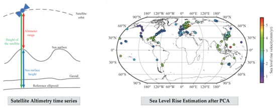
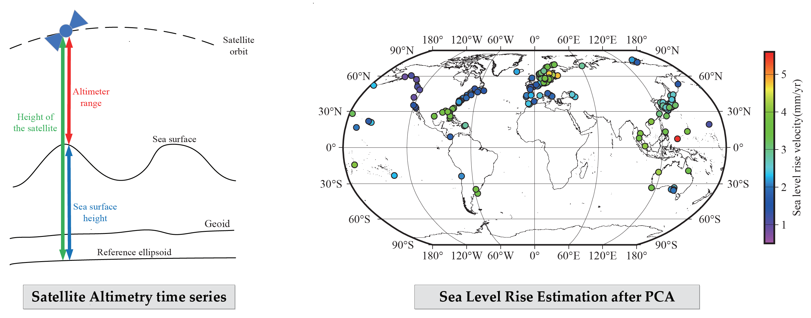
2.1. Satellite Altimetry and Sea Surface Height

The radar of the satellite altimeter operates by measuring the time for signals to propagate between the satellite’s elevation and the surface of the sea. The difference and the SA altitude measured above a specified reference surface and the altimetric range result in the determination of SSH, as depicted in Figure 1. The discrepancy between the sea level and reference ellipsoid is illustrated in Figure 1 [19,20].

2.2. Sea Surface Height Observations from Copernicus

We used the daily global ocean physics reanalysis product of GLOB-AL_MULTIYEAR_PHY_001_030 (https://doi.org/10.48670/moi-00021, accessed on 6 March 2023) from the Copernicus Marine Environment Monitoring Service (CMEMS), covering the period from 1993 to 2020, which is defined on a standard regular grid at 1/12 degree resolution and covering approximately 8 km [13]. To investigate the sea level change in SSH from SA, we selected 184 sites around the coasts (also called virtual coastal stations with SA observations), as illustrated in Figure 2. In this study, we determined the 184 virtual coastal stations based on the longitude and latitude of the TG from PSMSL, and those TG stations corresponding to the selected virtual stations include at least 50 years of data. In addition, the virtual coastal stations should be distributed globally as evenly as possible. The virtual coastal stations have data spanning from 1993 to 2020. They cover a substantial number of coastal regions around the world.

2.3. Geophysical Fluid-Loading Product

The temporal changes in surface mass loading result in the elastic deformation of the Earth’s surface [21]. In this study, we utilized the geophysical fluid-loading products retrieved from the German Research Center for Geosciences to further reduce those seasonal effects. These products encompass the mass redistribution of hydrological loading (HYDL), non-tidal atmospheric loading (NTAL), sea level loading (SLEL), and non-tidal oceanic loading (NTOL), which caused seasonal deformations in the Earth’s surface. A more detailed and specific description of the 4 loading products is posted in http://rz-vm115.gfz-potsdam.de:8080/repository, accessed on 6 March 2023.

In this study, we employed a bicubic interpolation method to compute the environmental loading deformation at each station, utilizing latitude and longitude as the parameters. This approach aligns with the methodology outlined by Dill et al. (2013) [22]. It is important to acknowledge that atmospheric models, oceanic models, and hydrological models typically do not maintain global mass conservation. Notably, many oceanic models maintain a constant mass without accounting for mass exchange with the atmosphere and land. However, we used these models for noise reduction purposes rather than geophysical analysis, so this characteristic had no impact on the outcomes of our study.

2.4. Stochastic Noise Property of Sea Surface Height Time Series

Many geophysical time series, including the GNSS time series as well as the water level derived from tide gauges, suffer from time-correlated noise [23,24,25,26]. If sea level variations exhibit spatiotemporal correlations, these are frequently overlooked in SLR estimation for the sake of simplicity and/or ignorance, leading to potential consequences such as an underestimation of uncertainty. A few authors have tried to perform noise analysis, such as Nerem et al. (2010), who conducted a sea level data merging of all SA missions, and the effect of color noise on the estimated rate uncertainty was found to be lower than 0.1 mm/yr, 0.12 mm/yr, and 0.20 mm/yr using various noise models including autoregressive (AR)/AR fractionally integrated (ARFI)/generalized Gauss–Markov (GGM) stochastic models [27]. Bos et al. (2014) further analyzed the stochastic noise model and its accuracy for sea level time series and found an underestimation of the rate uncertainty in the case of a white noise (WN) assumption [9].

The literature suggests that autocorrelation significantly magnifies the uncertainty estimates linked to formal trends, consequently affecting the confidence in drawing conclusions about the identification of sea level acceleration. In this work, we examined stochastic noise with a time-varying seasonal signal from the linear trend estimation of the sea level data described in the previous section [28,29]. We selected the autoregressive moving average (ARMA) (p, q); ARFIMA (p, d, q); GGM; flicker and white noise (FNWN); random walk, flicker, and white noise (RWFNWN); and power law and white noise (PLWN) models following Montillet et al. (2018), Wöppelmann et al. (2012), and He et al. (2017, 2019) with the package Hector (with access of https://teromovigo.com/hector/ (accessed on 6 March 2023) or https://pypi.org/project/hectorp/0.1.7/ (accessed on 6 March 2023)) [26,30,31,32]. To accurately model the stochastic noise properties of the SSH time series from SA, we employed the optimal noise model selection criterion called BIC_tp, as described in He et al. (2019) [32]. Additionally, the power spectral density (PSD) plot was utilized for visual control as outlined in Bos et al. (2014) and He et al. (2017) [9,26]. Thus, we aimed to accurately assess the stochastic noise in a sea level time series.

2.5. Common Mode Noise Reduction with Principal Component Analysis

As outlined by Wdowinski et al. (1997), spatiotemporal correlated noise (also called common mode noise) is inherent in regional or global geodetic networks, such as GNSS, and sea level time series networks [9,33]. This noise, commonly referred to as common mode noise, has been previously discussed in the work of various authors [8,26,34,35,36].

Principal component analysis (PCA) has been proposed as a solution for the common mode noise from multiple time series (e.g., Aubrey and Emery, 1986; Dong et al., 2006) and was applied by Burgette (2013), who underlined that the PCA should perform more effectively on records of a consistent length and with complete datasets [8,34,37]. We proposed the use of a similar approach for the virtual network derived from SA observations. Our examined SA time series were optimal for reaching that goal as they spanned from 1993 to 2021 with an average data gap of 0.41% and a maximum data loss of 2.09%. We applied the PCA method to the SSH time series to reduce the spatiotemporal correlation noise in the related sea level time series derived from the downloaded SA ocean reanalysis product. The data processing is explained in the next section in detail. In addition, we uploaded the theory and program related to noise reduction with principal component analysis on SA time series to https://www.kaggle.com/datasets/spacegeodesy/sa-tool-v1-0-for-sa-on-sea-level-rise-estimation (see “Theory of PCA on SA noise reduction.pdf”) (accessed on 6 March 2023).

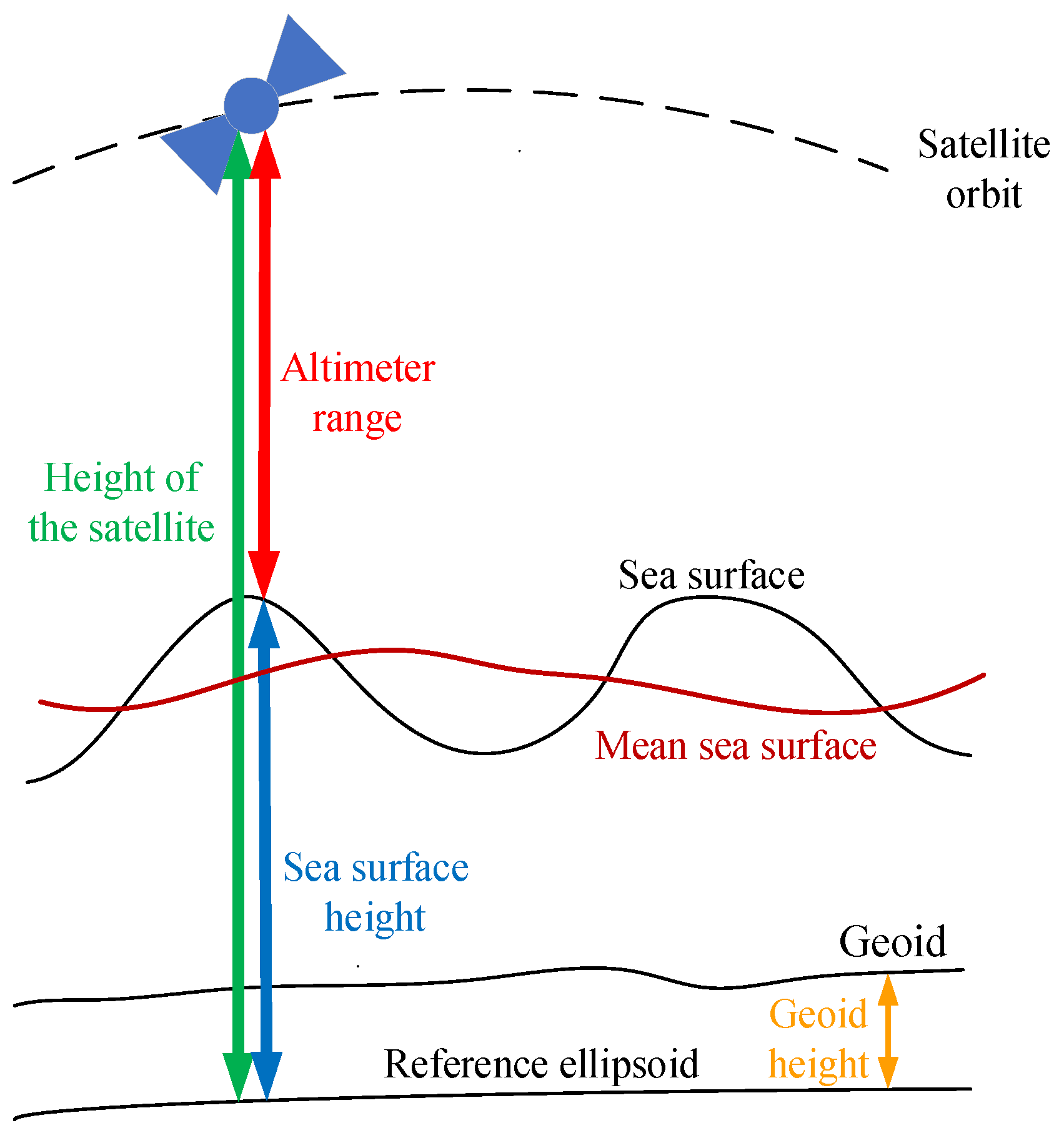
2.6. Toolbox for Sea Surface Hight Processing and Analysis

In the realm of processing raw SA ocean reanalysis product in NetCDF format [38], we created the Satellite Altimetry Toolbox (SA_Tool V1.0). Accessible at https://www.kaggle.com/datasets/spacegeodesy/sa-tool-v1-0-for-sa-on-sea-level-rise-estimation (accessed on 10 April 2023), this MATLAB GUI-based toolkit facilitates the processing and analysis of SA data. As illustrated in Figure 3, SA_Tool V1.0 encompasses three pivotal modules: the SA NetCDF to grid point module, the Data Preparation module, and the SSH TS Denoise module. SA_Tool V1.0 offers versatile functionalities, including reading raw NetCDF-format SA observations, generating SSH time series at specified points given their latitude and longitude, outlier detection using 3IQR, interpolation of SSH time series, and applying PCA filtering to the SSH time series. SA_Tool’s modules operate independently, allowing users to execute each model separately. Simultaneously, a well-defined interconnection exists between the modules, enabling the output of one module to serve as input data for another. The seamless integration and synergy between these modules create comprehensive time series processing and analysis software. The “Trend Analysis on SSH Time Series with PCA” section delves into the mathematical models and fundamental functions of each module, offering in-depth insights into the toolkit’s capabilities.

3. Results

3.1. Stochastic Noise Property Analysis of SSH Time Series

For the stochastic noise property analysis of the SSH time series, we analyzed 184 SA virtual coastal stations (Figure 2) using the stochastic models described in the previous section. Figure 4 displays examples of the SSH time series of the 0009 (NLD), 0636 (USA), 1027 (JPN), and 1325 (CAN) sites. The SSH time series exhibit significant seasonal fluctuations (e.g., 1027 and 1325 show an obvious sinusoidal signal) and an envelope corresponding to slow variations. In addition, slight differences in the periodic signal changes (e.g., amplitude of the seasonal signal) of the four listed sites are visible in Figure 4, highlighting regional differences in the SSH time series.

Previous studies have pointed out that a geometric time series can be modeled with correlated (also called colored) noise, and that different stochastic models have a significant impact on velocity parameter estimation for GNSS displacement time series [23,24,32,38]. To explore the optimal noise model of the SSH time series and the related impact, we used the ARMA (p, q), ARFIMA (p, d, q), GGM, FNWN, PLWN, and RWFNWN stochastic models to fit the SSH time series. We estimated the time-varying seasonal signal using the software Hector V2.1 based on maximum likelihood estimation as described in Bennett (2008) and Bos et al. (2013) [12,28]. Figure 5 shows the PSD of SSH residuals when various stochastic models were considered during the estimation. The stochastic models FNWN/RWFNWN/PLWN exhibit a poorer fit to the SSH time series, whereas the GGM, ARMA (1, 1), and ARFIMA (1, d, 1) models demonstrate a better result for the SSH time series of SA virtual coastal stations 0202/1299, 0819/0413, and 0485/0636, respectively.

In the second step, we compared the impact of various stochastic noise models from the SSH time series on the velocity and velocity uncertainty. The results are displayed in

Table A1. Velocity and velocity uncertainty estimated from SSH data under various models. (The optimal model for 0485/0636 station time series is ARFIMA (1, d, 1), The optimal model for 0413/0819 station time series is ARMA (1, 1), The optimal model for 0202/1299 station time series is GGM).

Value (mm/yr)	Site	ARFIMA (1, d, 1)	ARMA (1, 1)	GGM	FNWN	PLWN	RWFNWN
Velocity	0485	2.33	2.15	2.15	2.65	0.34	2.93
	0636	1.74	1.75	1.75	1.46	1.10	1.46
	0413	2.18	2.16	2.16	2.42	2.40	2.42
	0819	3.43	3.37	3.37	2.75	2.86	2.75
	0202	1.51	1.46	1.45	1.43	1.46	1.43
	1299	1.63	1.81	1.79	1.38	1.47	1.38
Uncertainty	0485	0.41	0.17	0.16	1.09	314.41	55.45
	0636	0.70	0.31	0.36	6.21	21.21	6.21
	0413	0.40	0.35	0.37	5.30	2.85	5.30
	0819	0.21	0.29	0.30	8.03	3.11	8.03
	0202	0.52	0.18	0.23	2.40	1.86	2.40
	1299	0.64	0.17	0.25	2.00	1.38	2.00
Mean Uncertainty		0.48 ± 0.16	0.25 ± 0.07	0.28 ± 0.07	4.17 ± 2.51	57.47 ± 115.12	13.23 ± 19.00

. Under the ARMA and GGM stochastic model assumptions, the estimation results of the SSH velocity parameters are close, and show only a slight difference compared to the ARFIMA model. As expected, the velocity uncertainty with ARFIMA becomes larger than that for the ARMA and GGM models, which is linked to the long-range dependency (long-term correlations) due to the time-varying amplitude of the periodical components [39]. The estimated velocity uncertainty is higher for the poor-fit noise models, e.g., 8.03, 314.41, and 55.45 mm/yr for FNWN, PLWN, and RWFNWN, respectively. These velocity uncertainties are unrealistic and linked with the unbounded increase in the variance at low frequency. The six sites listed in Table A1 did not select FNWN/FNRWWN/PLWN as optimal noise models but did select the ARMA (1, 1)/ARFIMA (1, d, 1)/GGM models. However, the value of (p, d, q) in the ARFIMA and ARMA models will affect the velocity estimation and uncertainty. As an example, Bos et al. (2014) found rate uncertainties of 0.02 mm/yr and 0.03 mm/yr with AR (1) and AR (5), respectively [9]. Figure 6 and Figure A1 show the statistical analysis of the average absolute value of velocity difference on the 184 sites using the ARFIMA (p, d, q) and ARMA (p, q) models (p ∈ (0,5), q ∈ (0,5)) and comparing the velocity parameters with the ARFIMA (1, d, 1) and ARMA (1, 1) models. We can see that the difference between the ARMA and ARFIMA models is small, with a maximum velocity difference of 0.11 mm/yr. The results for the uncertainty are presented in

Table A2. Statistical analysis of velocity uncertainty ratio with different stochastic models ((p ∈ (0,5), q ∈ (0,5))).

Uncertainty Ratio	$\frac{\mathit{A}\mathit{R}\mathit{F}\mathit{I}\mathit{M}\mathit{A}(\mathit{p},\mathit{d},\mathit{q})}{\mathit{A}\mathit{R}\mathit{F}\mathit{I}\mathit{M}\mathit{A}(1,\mathit{d},1)}$	$\frac{\mathit{A}\mathit{R}\mathit{M}\mathit{A}(\mathit{p},\mathit{q})}{\mathit{A}\mathit{R}\mathit{M}\mathit{A}(1,1)}$
Max	2.07	1.27
Min	0.82	0.92
Mean	0.93	1.16

. Under the ARFIMA and ARMA models, the velocity uncertainty varies around factors of 0.82~2.07 and 0.92~1.27. This difference illustrates that an accurate estimation of the (p, q) values is of considerable importance to obtain an accurate velocity with the corresponding reliable uncertainty from the SSH time series.

In the following, we utilize the GGM, ARMA (p, q), and ARFIMA (p, d, q) models through varying p and q between 0 and 5 for the 184 SA virtual coastal stations. We use the BIC_tp criterion which was chosen with a higher confidence as the optimal noise model for the functional model of interest (trend and seasonal components), as highlighted in the work of He et al. (2019) [32]. The results show that 54.9%, 41.3%, and 3.8% of the sites are best described using the ARFIMA (p, d, q), ARMA (p, q), and GGM models. Among them, ARFIMA (1, d, 1), ARFIMA (3, d, 0), and ARFIMA (1, d, 2), and ARMA (2, 2), ARMA (1, 2), and ARMA (1, 1) account for the highest proportion for ARFIMA and ARMA, respectively. In addition, we illustrate the spatial arrangement of the optimal stochastic model using the analyzed time series of sea surface height (SSH) across 184 virtual coastal stations in Figure 7. No obvious patterns allow for classification with an optimal noise model. This outcome is reasonable, because each virtual station may differ as to the data quality.

3.2. Geophysical Fluid-Loading Effect of SSH Time Series

In this section, we investigate the extent to which geophysical loading products would affect the SLR and its uncertainty. Figure A2 shows the statistical distribution of the maximum and mean values of the amplitude of the combined HYDL, NTAL, NTOL, and SLEL loading deformation between 1993 and 2020 for the 184 stations of the virtual network.

The histogram in Figure A2 (left, max value) highlights that the combined HYDL, NTAL, NTOL, and SLEL loading-induced sea surface variation can reach up to 30 mm. Thus, the geophysical loading effect is significant for a short time series, while it is close to zero on average for a long time series (mean of 28 years). This result is due to the strong seasonal component of the loading products.

We further investigated the impact of geophysical fluid loadings through a reduction in the raw SSH time series. Figure 8 shows the statistical distribution of the correlation coefficients of the analyzed SSH time series with respect to the geophysical loading products’ time series, i.e., the four combined loading-induced height time series. Figure 8 highlights that the mean value of the correlation coefficients for the 184 virtual stations is −0.30, and the maximum and minimum values of the correlation coefficient are 0.20 and −0.78, respectively. Most virtual stations show a negative correlation and the correlation coefficient is small. Furthermore, after loading correction, about 88.0% of the selected optimal noise model remains unchanged.

We further showed that the root mean square (RMS) of the SSH time series after reduction increases slightly, i.e., about 82.1% of the sites displayed an average increase of around 0.66 mm. Thus, the impact of the geophysical fluid-loading products on the SSH time series is relatively small and can be ignored. Furthermore, we evaluated the impact of geophysical fluid loading on the estimation of sea level trend parameters. From Figure A3, we concluded that geophysical fluid loading has a small effect on velocity estimation, with about 80.5% of sites displaying a velocity difference below 0.10 mm/yr.

Table 1. Velocity uncertainty difference ($Uncertaint{y}_{Loading}-Uncertaint{y}_{Raw}$).

Difference [mm/yr]	Proportion
<0	22.3%
0~0.2	75.0%
>0.2	2.7%

shows the velocity uncertainty difference ($Uncertaint{y}_{Loading}-Uncertaint{y}_{Raw}$) with and without loading correction. After correction, the uncertainty of about 77.7% of the sites is larger than in the raw case for SSH time series. Correspondingly, the effects of reducing the raw SSH time series from geophysical fluid loading are small compared to what was discovered for the GNSS time series [40]. We absolutely believe that geophysical fluid loading is not appropriate for SSH time series potentially, due to their time-varying amplitude and/or local effects that are not accounted for in the products. We propose to renounce their use for SSH time series derived from SA observations.

3.3. Trend Analysis on SSH Time Series with PCA

To mitigate the noise in the SSH time series, we used the PCA method to eliminate common mode noise shared temporally and spatially within the network of the analyzed SA virtual coastal stations. The noise reduction process is summarized in brief as follows (see Figure 9):

(1) Data Preprocessing. Detect offsets using the “find_offset.py” module of Hector and eliminate outliers through the three-times interquartile range rule (IQR) [12,13];

(2) Data Interpolation. For PCA analysis, complete datasets with no gaps are necessary [8]. We utilized regularized expectation-maximization (ReGEM) to interpolate the missing data into the satellite altimetry time series. ReGEM involves iterated analyses of linear regressions, considering variables with missing values in relation to those with available values. This method accounts for correlation and physical background between time series, offering more accurate estimates of the missing values [41];

(3) Detrend and noise reduction. Remove linear trends with the least square method, then perform common mode noise reduction with PCA on the residual SSH time series. We followed the indicators that the stations (>50.0%) had clearly normalized responses (>25.0%) as recommended by Dong (2006) [34].

Figure 10 shows the spatial response of the first three PCs after applying the PCA noise reduction algorithm to the SSH time series. The value of the spatial response for PC1 was more than 25.0% for most of the SSH time series and PC1 had a mean spatial response value of 26.3% for the 184 stations analyzed. For PC2 and PC3, most stations have a positive spatial response, while the average valued of PC2 and PC3 were 12.4% and 0.9% for SSH, respectively. The spatial response of PC1 displays a good consistency compared with that of PC2 and PC3. The percentage of the first 11 PC eigenvalues sorted from low to high PC orders on SSH times series are shown in

Table A3. Individual contribution rate of the first 11 eigenvalues sorted according to the PC order.

PCs	SSH
	Contribution Rate (%)
1	28.0
2	15.1
3	8.7
4	7.9
5	6.7
6	3.9
7	2.7
8	2.2
9	2.1
10	2.0
11	1.9

. The first PC accounts for 28.0% of the SSH time series, implying that the first PC may represent the common variation in the network. The standard of the CME definition is examined in reference [34], in which the stations (>50.0%) had clearly normalized responses (>25.0%). Thus, the first PC models can be defined as the common mode noise of the entire network of SSH time series.

After removing common mode noise through PCA, the RMS of 96.7% of the SSH times series decreases by an average of 8.47 mm, and the average correlation coefficient of the SSH times series before and after noise reduction is 0.86. In addition, after PCA noise reduction, about 51.6% of the SSH time series’ optimal noise model changes. We then used the optimal noise models to compare the velocity parameters before and after applying the PCA method.

Table 2. Distribution of velocity parameter variation on SSH time series after PCA noise reduction.

Difference	Interval Distribution
Velocity |Raw − PCA|	[0.00, 0.10]	(0.10, 0.20]	>0.20
	81.0%	9.8%	9.2%
Uncertainty (PCA − Raw)	<0	[0, 0.2]	>0.2
	59.3%	31.5%	9.2%

provides the distribution of variations in the velocity parameters after PCA noise reduction. The results show that PCA preserves the velocity of the original SSH time series, while the velocity uncertainty’s accuracy improves after PCA denoising (about 59.3% of virtual coastal stations’ velocity uncertainty is reduced). It should be mentioned that our stations were not chosen to provide the most favorable results, so this result highlights the importance of PCA denoising to improve SLR retrieval (both parameters and uncertainty).

4. Discussion: SLR Change Estimated from SA

In this section, we analyze the SLR change estimated from the SSH time series after PCA noise reduction. In Figure 11, the velocity of the SLR change for the 184 virtual coastal stations analyzed is illustrated, with data spanning the period 1993 to 2020. To assess the spatial and temporal fluctuations in sea level change, we divided the 28-year-long SSH time series into four time periods: 1993–2006, 2000–2013, 2006–2020, and 1993–2020.

Table A4. Statistical results of velocity and related uncertainty for different periods.

Values	Period	Mean
Velocity (mm/yr)	1993–2006	2.46 ± 1.83
	2000–2013	3.02 + 1.41
	2007–2020	3.02 ± 2.10
	1993–2020	2.75 ± 0.89

shows the statistical results of velocity and related uncertainty for different periods, highlighting that the rate of SLR in the past 14 years (2006–2020 with mean rate of 3.02 ± 2.10 mm/yr) has been significantly higher than in the previous 14 years (1993–2006 with mean rate of 2.46 ± 1.83 mm/yr) for the 184 virtual coastal stations analyzed. Using a long-term time series is beneficial for the accuracy of the estimated parameters, e.g., with 14 years of data, the uncertainty is around 1.8 mm/yr, and it decreases to around 0.89 mm/yr with 28 years of data. Note that in the appendices,

Table A5. Statistics results for velocity in four regions from 1993 to 2020.

Area	Number	Velocity
1	16	1.61 ± 0.67
2	34	2.49 ± 0.81
3	67	2.92 ± 0.91
4	55	3.00 ± 0.65
5	12	2.96 ± 0.79

shows the SLR estimated for various regions.

The geocentric ocean height rates (also referred to as GMSL) observed in the twentieth century exhibited a global mean of 1.5~1.9 mm/yr. This is approximately half the rate observed in the twenty-first century, which is 3.2 [2.8~3.6] mm/yr. This discrepancy implies a continuing acceleration in the rates of sea level rise [42,43]. We found a value of 2.75 ± 0.89 mm/yr for the SLR. This is lower than the estimates of Cazenave et al. (2018) with 3.1 ± 0.3 mm/yr, and Horwath et al. (2021) with a value of 3.3 ± 0.4 mm/yr [44,45,46]. This is because we did not apply glacial isostatic adjustment (GIA) in sea level rise trend estimation, and GIA for GMSL is about −0.3mm/yr. Dangendorf et al. (2019) averaged the SLR of eight regions, and identified that RSLR ranged from 0.2 to 3.5 mm/yr with a global mean of around 2.8 ± 0.1 mm/yr [5]. Therefore, our estimate is at the low end of the interval of values defined for the twenty-first century rates. However, our associated uncertainty is high, i.e., more than twice the uncertainties associated with the previous GMSL values. We can explain this discrepancy by considering the following:

a. The 184 virtual coastal stations analyzed are all based on the longitude and latitude of TG sites from PSMSL, which are close to the coastline and have significant fluctuations in sea level, making the uncertainty of the rate higher. We further chose the virtual stations without searching for optimality. Thus, the coherence of our results with previous findings highlights the importance of an accurate stochastic model and a PCA reduction;

b. The CMEMS ocean reanalysis product may have slightly lower accuracy in offshore areas, and further studies on the consistency of uncertainty in satellite estimates of global mean sea level changes from Copernicus/AVISO/CORA2.0 SA products are needed in the future;

c. We modeled the time correlations within the observations with the colored noise models (ARMA/ARFIMA/GGM). Therefore, we increased the uncertainty to take into account the noise amplitude and long-range dependency intrinsic to the data, but also to enhance the reliability of the results.

5. Conclusions

We have investigated the spatiotemporal pattern of SSH time series with 184 globally distributed virtual coastal stations around the coast with data ranging between 1993 and 2020. We have carefully analyzed the stochastic noise properties and their effect on the computed SLR based on the BIC_tp criterion and evaluated the geophysical fluid-loading effect on the SSH time series. Finally, spatiotemporal filtering with PCA has been performed to mitigate the common mode noise. The following conclusions can be drawn:

(1) We have analyzed the stochastic noise properties of the SSH time series with the BIC_tp criterion under the background noise modes of ARFIMA (p, d, q), ARMA (p, q), GGM, FNWN, PLWN, and RWFNWN, and explored the influence of different types of noise on the velocity parameters of the SSH time series. Our results show that the FNWN, PLWN, and RWFNWN misfit the correlated noise of the SSH time series. We conclude that the SSH time series can be best described with the ARMA/ARFIMA/GGM models, which account for long-term correlated noise. In addition, the accurate estimation of the (p, q) values is of great importance to obtain trustworthy SSH time series velocity parameters.

(2) For the first time, we have investigated the impact of geophysical fluid loading for SSH data on the sea level change. The results show that the correlation coefficients between the SSH time series and the combined HYDL, NTAL, NTOL, and SLEL loading-induced sea surface variation time series are negative and small. Therefore, the geophysical fluid-loading products are not appropriate for correcting the SSH time series.

(3) After removing the common mode noise in the SSH data with PCA, 96.7% of the times series’ RMS decreases (with an average of 8.47 mm reduction), and the average correlation coefficient before and after noise reduction is around 0.86. Most of the uncertainty associated with the computed SLR after applying PCA decreases.

(4) We have estimated the SLR change using four time periods: 1993–2006, 2000–2013, 2006–2020, and 1993–2020. We have observed that the SLR increases at a mean rate of 2.75 ± 0.89 mm/yr between 1993 and 2020, which is at the low end of the interval of [2.8–3.6] mm/yr defined by the IPCC.

We have introduced to the community an open-source software program (SA_Tool V1.0) to process SA data and reduce noise in surface height time series. Overall, we support the findings of Cazenave et al. (2018), Horwath et al. (2021) and Camargo et al. (2023) [44,45,46]. However, our selected virtual stations do not cover all of the world’s coastlines. Therefore, we must be careful when comparing our estimates with those of other studies. In addition, most of our virtual coastal stations are located close to the coastline. Sea level observation from SA has faced difficulties, e.g., the influence of coastal bottom topography and water dynamics poses challenges in directly extracting useful information from the waveform in coastal areas. This difficulty contributes to a decrease in data accuracy [47].

References

1. Church, J.A.; White, N.J. Sea-level rise from the late 19th to the early 21st century. Surv. Geophys. 2011, 32, 585–602. [Google Scholar] [CrossRef]
2. Nerem, R.S.; Beckley, B.D.; Fasullo, J.T.; Hamlington, B.D.; Masters, D.; Mitchum, G.T. Climate-change–driven accelerated sea-level rise detected in the altimeter era. Proc. Natl. Acad. Sci. USA 2018, 115, 2022–2025. [Google Scholar] [CrossRef]
3. Van de Wal, R.S.W.; Zhang, X.; Minobe, S.; Jevrejeva, S.; Riva, R.E.M.; Little, C.; Richter, K.; Palmer, M.D. Uncertainties in long-term twenty-first century process-based coastal sea-level projections. Surv. Geophys. 2019, 40, 1655–1671. [Google Scholar] [CrossRef]
4. Frederikse, T.; Landerer, F.W.; Caron, L.; Adhikari, S.; Parkes, D.; Humphrey, V.; Dangendorf, S.; Hogarth, P.; Zanna, L.; Cheng, L.; et al. The causes of sea-level rise since 1900. Nature 2020, 584, 393–397. [Google Scholar] [CrossRef]
5. Dangendorf, S.; Hay, C.; Calafat, F.M.; Marcos, M.; Piecuch, C.G.; Berk, K.; Jensen, J. Persistent acceleration in global sea-level rise since the 1960s. Nat. Clim. Chang. 2019, 9, 705–710. [Google Scholar] [CrossRef]
6. Edwards, T.L.; Nowicki, S.; Marzeion, B.; Hock, R.; Goelzer, H.; Seroussi, H.; Jourdain, N.C.; Slater, D.A.; Turner, F.E.; Smith, C.J.; et al. Projected land ice contributions to twenty-first-century sea level rise. Nature 2021, 593, 74–82. [Google Scholar] [CrossRef]
7. Zhao, Q.; Pan, J.; Devlin, A.T.; Tang, M.; Yao, C.; Zamparelli, V.; Falabella, F.; Pepe, A. On the Exploitation of Remote Sensing Technologies for the Monitoring of Coastal and River Delta Regions. Remote Sens. 2022, 14, 2384. [Google Scholar] [CrossRef]
8. Burgette, R.J.; Watson, C.S.; Church, J.A.; White, N.J.; Tregoning, P.; Coleman, R. Characterizing and minimizing the effects of noise in tide gauge time series: Relative and geocentric sea level rise around Australia. Geophys. J. Int. 2013, 194, 719–736. [Google Scholar] [CrossRef]
9. Bos, M.S.; Williams, S.D.P.; Araújo, I.B.; Bastos, L. The effect of temporal correlated noise on the sea level rate and acceleration uncertainty. Geophys. J. Int. 2014, 196, 1423–1430. [Google Scholar] [CrossRef]
10. Royston, S.; Watson, C.S.; Legrésy, B.; King, M.A.; Church, J.A.; Bos, M.S. Sea-level trend uncertainty with Pacific climatic variability and temporally-correlated noise. J. Geophys. Res.-Oceans 2018, 123, 1978–1993. [Google Scholar] [CrossRef]
11. Woodworth, P.L.; Tsimplis, M.N.; Flather, R.A.; Shennan, I. A review of the trends observed in British Isles mean sea level data measured by tide gauges. Geophys. J. Int. 1999, 136, 651–670. [Google Scholar] [CrossRef]
12. Bos, M.S.; Fernandes, R.M.S.; Williams, S.D.P.; Bastos, L. Fast error analysis of continuous GNSS observations with missing data. J. Geodesy 2013, 87, 351–360. [Google Scholar] [CrossRef]
13. He, X.; Montillet, J.-P.; Fernandes, R.; Melbourne, T.I.; Jiang, W.; Huang, Z. Sea Level Rise Estimation on the Pacific Coast from Southern California to Vancouver Island. Remote Sens. 2022, 14, 4339. [Google Scholar] [CrossRef]
14. He, X.; Hua, X.; Yu, K.; Xuan, W.; Lu, T.; Zhang, W.; Chen, X. Accuracy enhancement of GPS time series using principal component analysis and block spatial filtering. Adv. Space Res. 2015, 55, 1316–1327. [Google Scholar] [CrossRef]
15. He, X.; Yu, K.; Montillet, J.-P.; Xiong, C.; Lu, T.; Zhou, S.; Ma, X.; Cui, H.; Ming, F. GNSS-TS-NRS: An Open-source MATLAB-Based GNSS time series noise reduction software. Remote Sens. 2020, 12, 3532. [Google Scholar] [CrossRef]
16. Burnham, K.P.; Anderson, D.R. Model Selection and Multimode Inference: A Practical Information-Theoretic Approach, 2nd ed.; Springer: New York, NY, USA, 2002. [Google Scholar]
17. Jones, I.F.; Levy, S. Signal-to-noise ratio enhancement in multichannel seismic data via the Karhunen-Loeve transform. Geophys. Prospect. 1987, 35, 12–32. [Google Scholar] [CrossRef]
18. Paterson, C. Practical Signal Processing and Its Applications; Springer: Berlin/Heidelberg, Germany, 2021; ISBN -13: 978-3030747281. [Google Scholar]
19. Cazenave, A.; Gouzenes, Y.; Birol, F.; Leger, F.; Passaro, M.; Calafat, F.M.; Shaw, A.; Nino, F.; Legeais, J.F.; Oelsmann, J.; et al. Sea level along the world’s coastlines can be measured by a network of virtual altimetry stations. Commun. Earth Environ. 2022, 3, 117. [Google Scholar] [CrossRef]
20. Chelton, D.B.; Schlax, M.G. The accuracies of smoothed sea surface height fields constructed from tandem satellite altimeter datasets. J. Atmos. Ocean. Technol. 2003, 20, 1276–1302. [Google Scholar] [CrossRef]
21. Jiang, W.; Li, Z.; van Dam, T.; Ding, W. Comparative analysis of different environmental loading methods and their impacts on the GPS height time series. J. Geodesy 2013, 87, 687–703. [Google Scholar] [CrossRef]
22. Dill, R.; Dobslaw, H. Numerical simulations of global-scale high-resolution hydrological crustal deformations. J. Geophys. Res. Solid Earth 2013, 118, 5008–5017. [Google Scholar] [CrossRef]
23. Langbein, J.; Johnson, H. Correlated errors in geodetic time series: Implications for time-dependent deformation. J. Geophys. Res. Solid Earth 1997, 102, 591–603. [Google Scholar] [CrossRef]
24. Mao, A.; Harrison, C.G.; Dixon, T.H. Noise in GPS coordinate time series. J. Geophys. Res. Solid Earth 1999, 104, 2797–2816. [Google Scholar] [CrossRef]
25. Baig, A.M.; Campillo, M.; Brenguier, F. Denoising seismic noise cross correlations. J. Geophys. Res. Solid Earth 2009, 114. [Google Scholar] [CrossRef]
26. He, X.; Montillet, J.-P.; Fernandes, R.; Bos, M.; Yu, K.; Hua, X.; Jiang, W. Review of current GPS methodologies for producing accurate time series and their error sources. J. Geodyn. 2017, 106, 12–29. [Google Scholar] [CrossRef]
27. Nerem, R.S.; Chambers, D.P.; Choe, C.; Mitchum, G.T. Estimating mean sea level change from the TOPEX and Jason altimeter missions. Mar. Geod. 2010, 33, 435–446. [Google Scholar] [CrossRef]
28. Bennett, R.A. Instantaneous deformation from continuous GPS: Contributions from quasi-periodic loads. Geophys. J. Int. 2008, 174, 1052–1064. [Google Scholar] [CrossRef]
29. Klos, A.; Bos, M.S.; Bogusz, J. Detecting time-varying seasonal signal in GPS position time series with different noise levels. GPS Solut. 2018, 22, 21. [Google Scholar] [CrossRef]
30. Montillet, J.P.; Melbourne, T.I.; Szeliga, W.M. GPS vertical land motion corrections to sea-level rise estimates in the Pacific Northwest. J. Geophys. Res.-Oceans 2018, 123, 1196–1212. [Google Scholar] [CrossRef]
31. Wöppelmann, G.; Marcos, M. Coastal sea level rise in southern Europe and the nonclimate contribution of vertical land motion. J. Geophys. Res.-Oceans 2012, 117. [Google Scholar] [CrossRef]
32. He, X.; Bos, M.S.; Montillet, J.P.; Fernandes, R.M.S. Investigation of the noise properties at low frequencies in long GNSS time series. J. Geodesy 2019, 93, 1271–1282. [Google Scholar] [CrossRef]
33. Wdowinski, S.; Bock, Y.; Zhang, J.; Fang, P.; Genrich, J. Southern California permanent GPS geodetic array: Spatial filtering of daily positions for estimating coseismic and postseismic displacements induced by the 1992 Landers earthquake. J. Geophys. Res. Solid Earth. 1997, 102, 18057–18070. [Google Scholar] [CrossRef]
34. Dong, D.; Fang, P.; Bock, Y.; Webb, F.; Prawirodirdjo, L.; Kedar, S.; Jamason, P. Spatiotemporal filtering using principal component analysis and Karhunen-Loeve expansion approaches for regional GPS network analysis. J. Geophys. Res. Solid Earth 2006, 111. [Google Scholar] [CrossRef]
35. He, X.; Bos, M.S.; Montillet, J.-P.; Fernandes, R.; Melbourne, T.; Jiang, W.; Li, W. Spatial variations of stochastic noise properties in GPS time series. Remote Sens. 2021, 13, 4534. [Google Scholar] [CrossRef]
36. Hu, Z.; Li, H.; Wang, D. Characterizing Tidal Currents and Guangdong Coastal Current Over the Northern South China Sea Shelf Using Himawari-8 Geostationary Satellite Observations. Earth Space Sci. 2023, 10, e2023EA003047. [Google Scholar] [CrossRef]
37. Aubrey, D.G.; Emery, K.O. Australia: An unstable platform for tide-gauge measurements of changing sea levels. J. Geodesy 1986, 94, 699–712. [Google Scholar] [CrossRef]
38. Farzaneh, S.; Parvazi, K. ATSAT: A MATLAB-based software for multi-satellite altimetry data analysis. Earth Sci. Inform. 2021, 14, 1665–1678. [Google Scholar] [CrossRef]
39. Langbein, J. Improved efficiency of maximum likelihood analysis of time series with temporally correlated errors. J. Geodesy 2017, 91, 985–994. [Google Scholar] [CrossRef]
40. Klos, A.; Dobslaw, H.; Dill, R.; Bogusz, J. Identifying the sensitivity of GPS to non-tidal loadings at various time resolutions: Examining vertical displacements from continental Eurasia. GPS Solut. 2021, 25, 89. [Google Scholar] [CrossRef]
41. Schneider, T. Analysis of incomplete climate data: Estimation of mean values and covariance matrices and imputation of missing values. J. Climate 2001, 14, 853–871. [Google Scholar] [CrossRef]
42. Hartmann, D.L.; Tank, A.M.G.K.; Rusticucci, M.J.I.A. IPCC fifth assessment report, climate change 2013: The physical science basis. Ipcc Ar5 2013, 5, 31–39. [Google Scholar]
43. Intergovernmental Panel on Climate Change. IPCC Special Report on the Ocean and Cryosphere in a Changing Climate; Pörtner, H.-O., Roberts, D.C., Eds.; IPCC: Geneva, Switzerland, 2019. [Google Scholar]
44. Cazenave, A.; Palanisamy, H.; Ablain, M. Contemporary sea level changes from satellite altimetry: What have we learned? What are the new challenges? Adv. Space Res. 2018, 62, 1639–1653. [Google Scholar] [CrossRef]
45. Horwath, M.; Gutknecht, B.D.; Cazenave, A.; Palanisamy, H.K.; Marti, F.; Marzeion, B.; Paul, F.; Le Bris, R.; Hogg, A.E.; Otosaka, I.; et al. Global sea-level budget and ocean-mass budget, with focus on advanced data products and uncertainty characterisation. Earth Syst. Sci. Data Discuss. 2021, 2021, 1–51. [Google Scholar] [CrossRef]
46. Camargo, C.M.L.; Riva, R.E.M.; Hermans, T.H.J.; Schütt, E.M.; Marcos, M.; Hernandez-Carrasco, L.; Slangen, A.B.A. Regionalizing the sea-level budget with machine learning techniques. Ocean Sci. 2023, 19, 17–41. [Google Scholar] [CrossRef]
47. Taqi, A.M.; Al-Subhi, A.M.; Alsaafani, M.A.; Abdulla, C.P. Improving sea level anomaly precision from satellite altimetry using parameter correction in the Red Sea. Remote Sens. 2020, 12, 764. [Google Scholar] [CrossRef]
Figure 1. The measure of the sea surface height using a radar installed on a satellite altimeter.
Remotesensing 16 01334 g001
Figure 2. Distribution of the 184 virtual coastal stations where the SSH time series are computed. Red circles-area 1 (West Coast of North America), blue circles-area 2 (West Coast of North America), green circles-area 3 (Europe), purple circles-area 4 (Western Pacific), and yellow circles-area 5 (Southern Hemisphere Station).
Remotesensing 16 01334 g002
Figure 3. Main interface of sea surface sight processing and analysis toolbox.
Remotesensing 16 01334 g003
Figure 4. SSH time series from the CMEMS SA ocean reanalysis product.
Remotesensing 16 01334 g004
Figure 5. The PSD of SSH time series with various stochastic models.
Remotesensing 16 01334 g005
Figure 6. Statistical analysis of absolute value of the velocity difference of ARFIMA models.
Remotesensing 16 01334 g006
Figure 7. Optimal stochastic model distribution of the 184 virtual coastal stations analyzed.
Remotesensing 16 01334 g007
Figure 8. The correlation coefficient distribution between SSH time series after load correction and the geophysical fluid-loading deformation.
Remotesensing 16 01334 g008
Figure 9. The flowchart of common mode noise reduction with PCA on SSH time series.
Remotesensing 16 01334 g009
Figure 10. (ac)Spatial responses of top 3 PCs of virtual coastal satellite altimetry stations.
Remotesensing 16 01334 g010
Figure 11. The spatial distribution of the velocity of the SLR change for the 184 virtual coastal stations analyzed, with data spanning the period from 1993 to 2020.
Remotesensing 16 01334 g011