


Climate Interprets Saturation Value Variations Better Than Soil and Topography in Estimating Oak Forest Aboveground Biomass Using Landsat 8 OLI Imagery

 , , , ,
Abstract
:
1. Introduction
- Clarify the relationships between the OSVs and climate, topographic, and soil variables.
- Identify the key environmental variables that determine the variations in the OSVs.
- Explore the interactive and comprehensive effect of the three types of environmental factors on the variation in the OSVs.
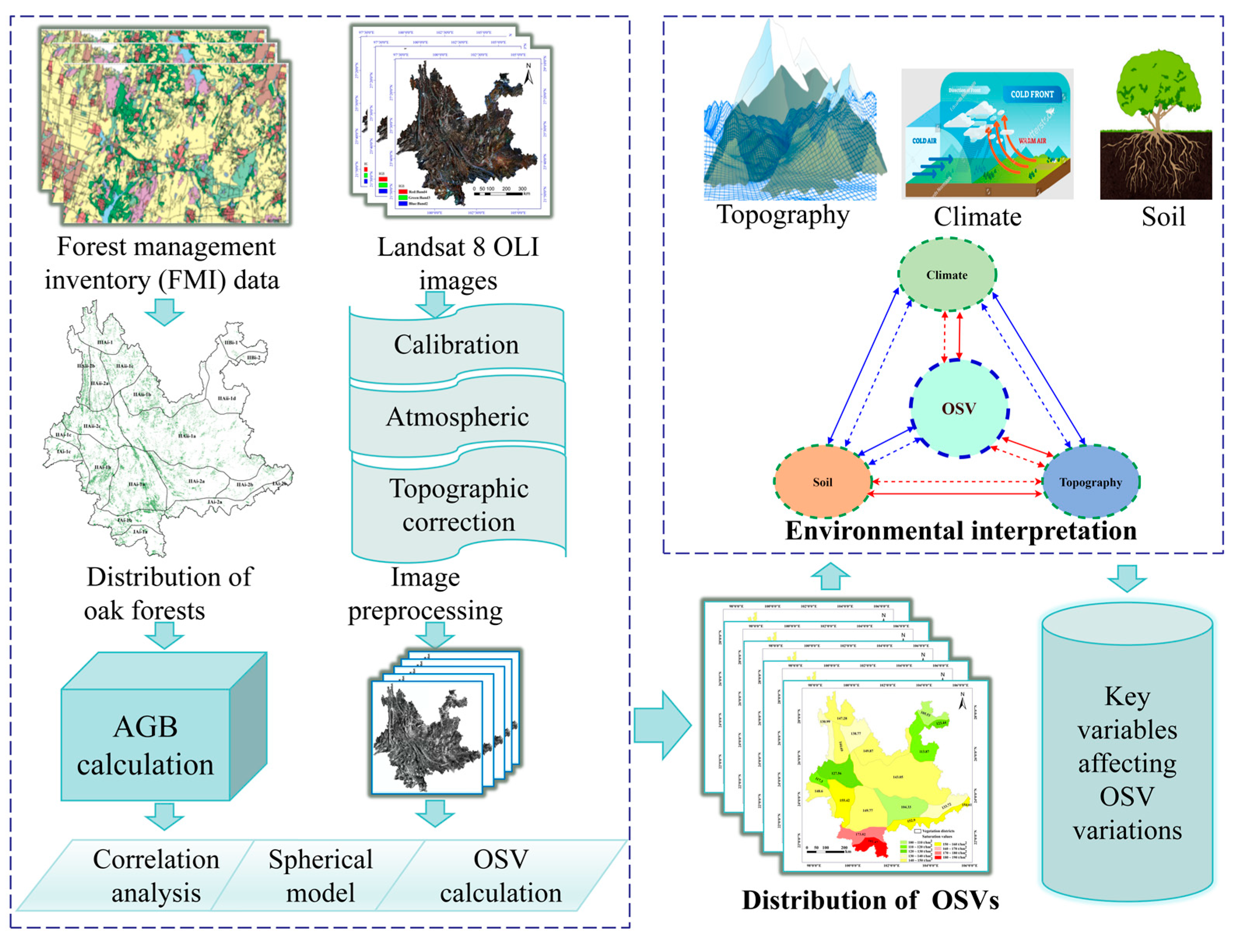
2. Materials and Methods
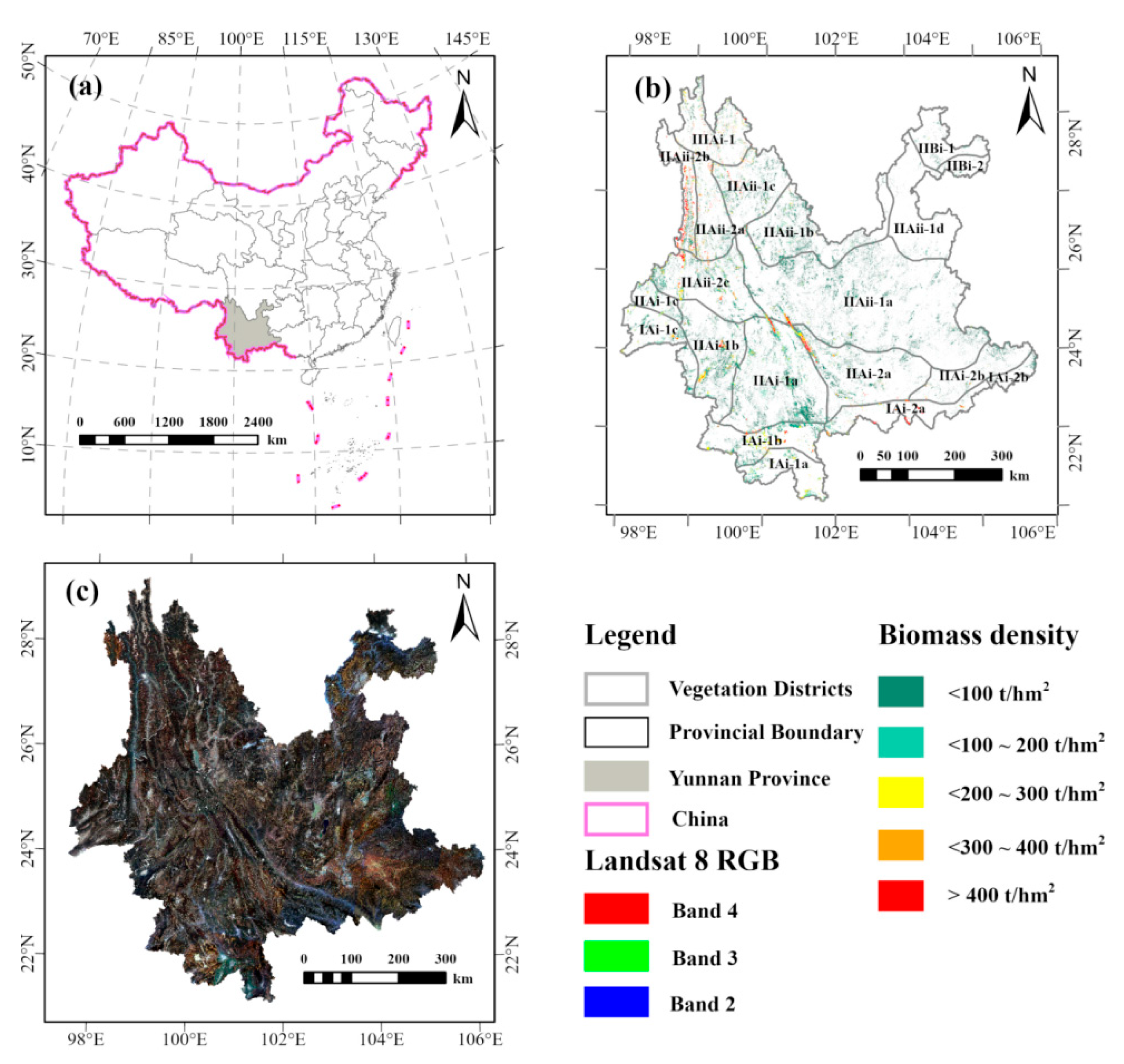
2.1. Study Area and Objects
2.2. Vegetation Districts in Yunnan Province
2.3. Forest Inventory Data Collection and Processing
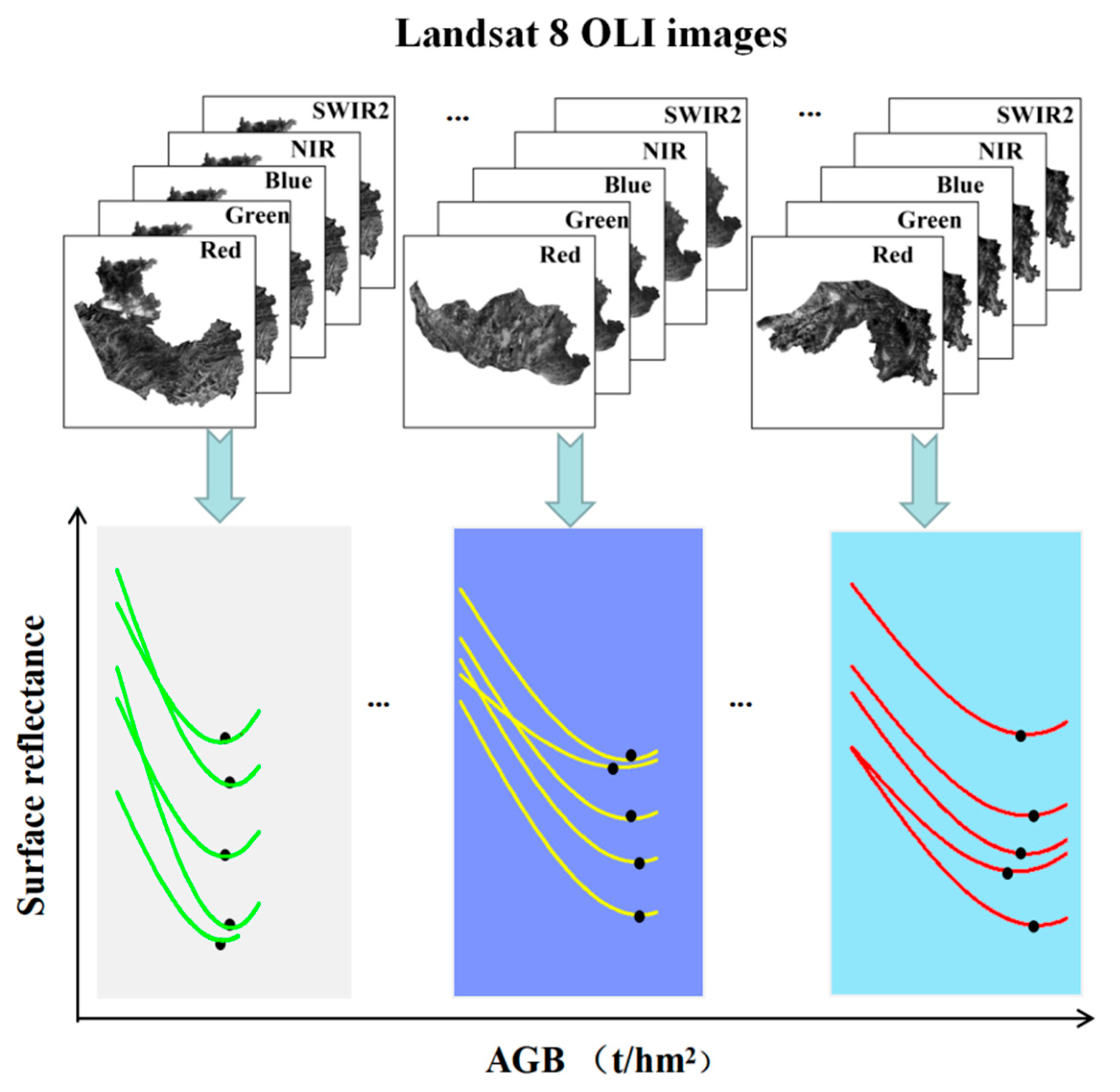
2.4. Remote Sensing Data: Access and Processing
2.5. Extracting Environment Factors
2.6. Band Screening and Obtaining OSVs
2.7. OSV Variation Analysis and Environmental Interpretation
2.7.1. Environmental Variables Screening
2.7.2. Analysis of the Environment Effect on OSV Variation
3. Results
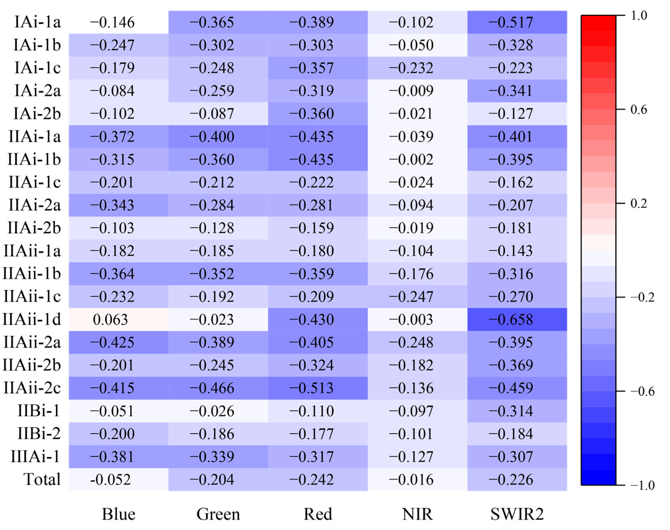
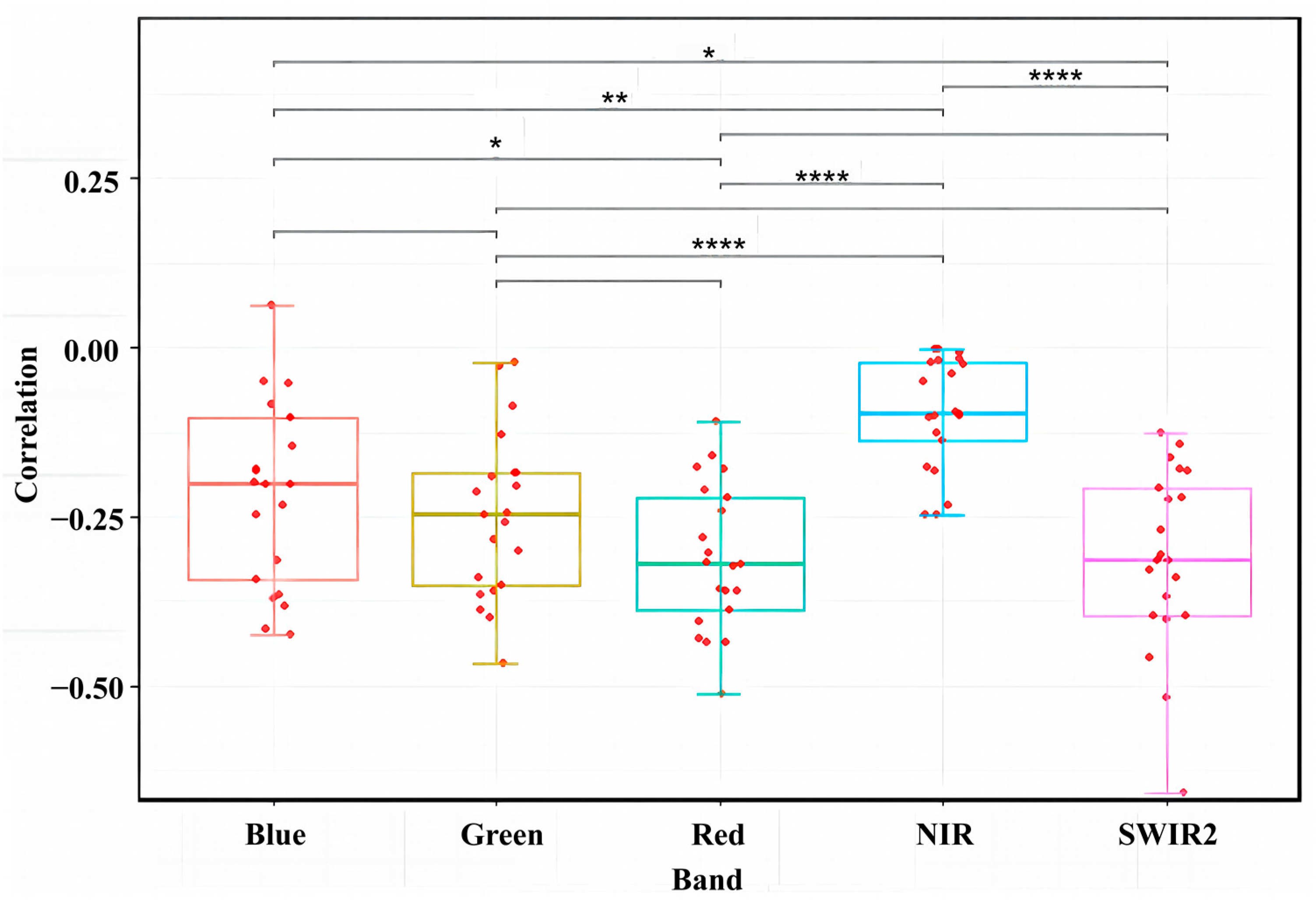
3.1. Correlation between the Bands and Oak Forest AGB
3.2. Variation Analysis of the OSVs
3.3. Relationships between the Environmental Factors and OSV Variation
4. Discussion
4.1. OSV Variation
4.2. Individual Environment Effect on OSV Variation
4.3. Interactive Effect of Environmental Factors on the OSV Variation
4.4. Comprehensive Effect of Environmental Factors on the OSV Variation
4.5. Application and Future Research
5. Conclusions
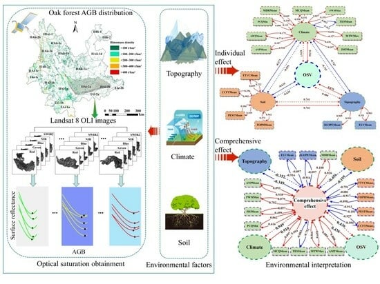
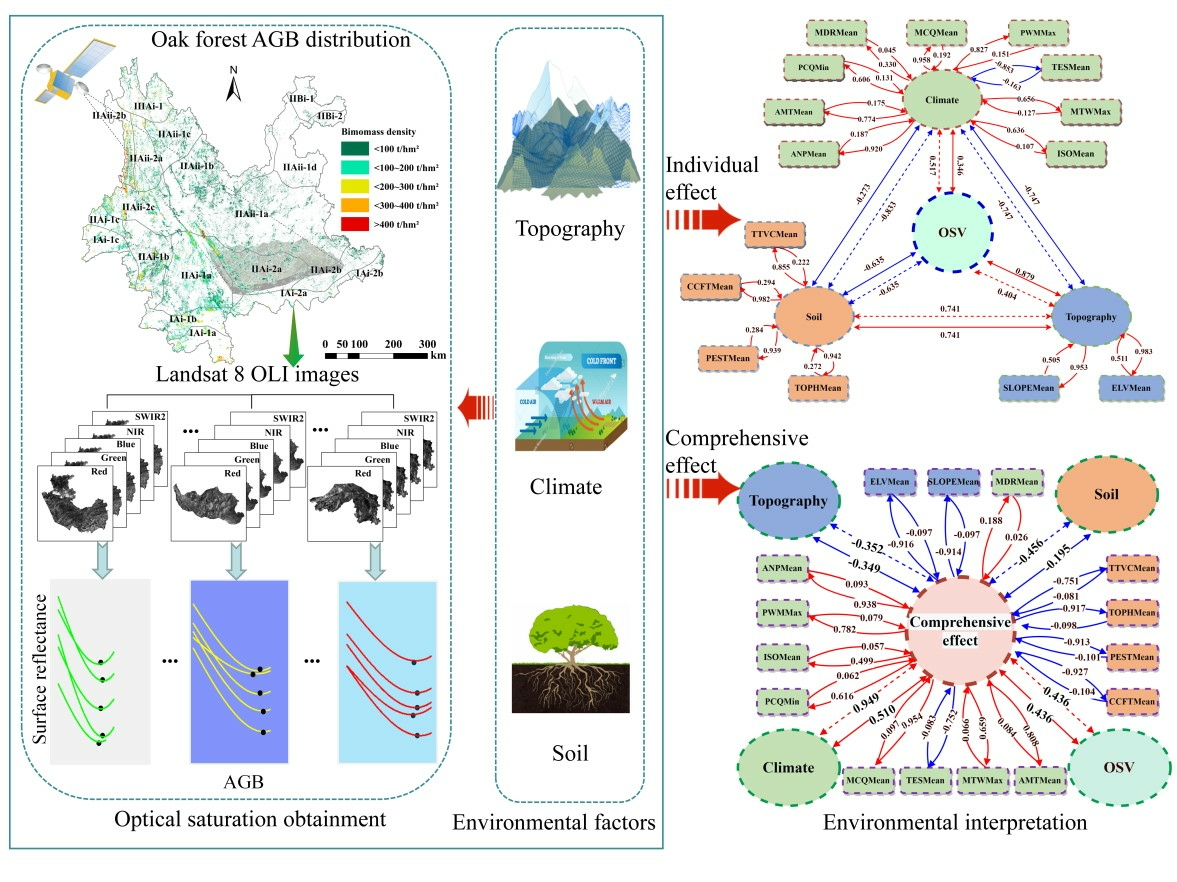
- (1)
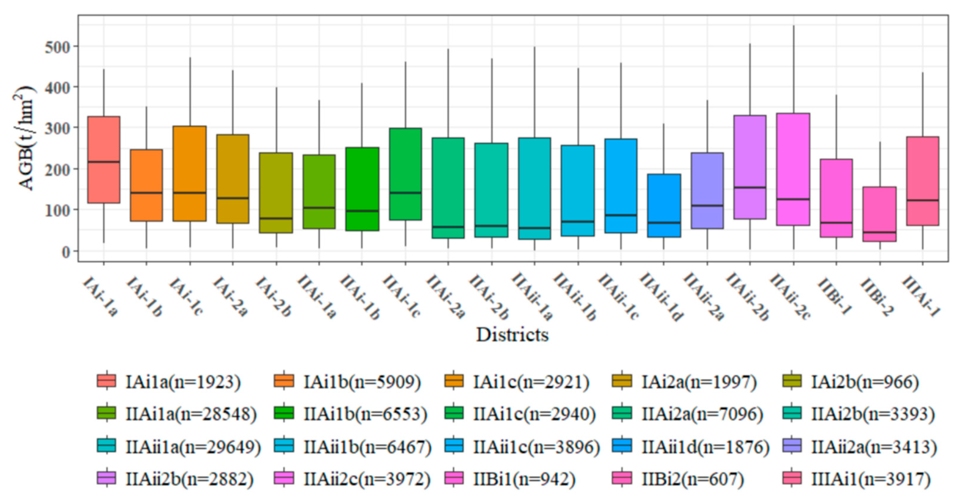
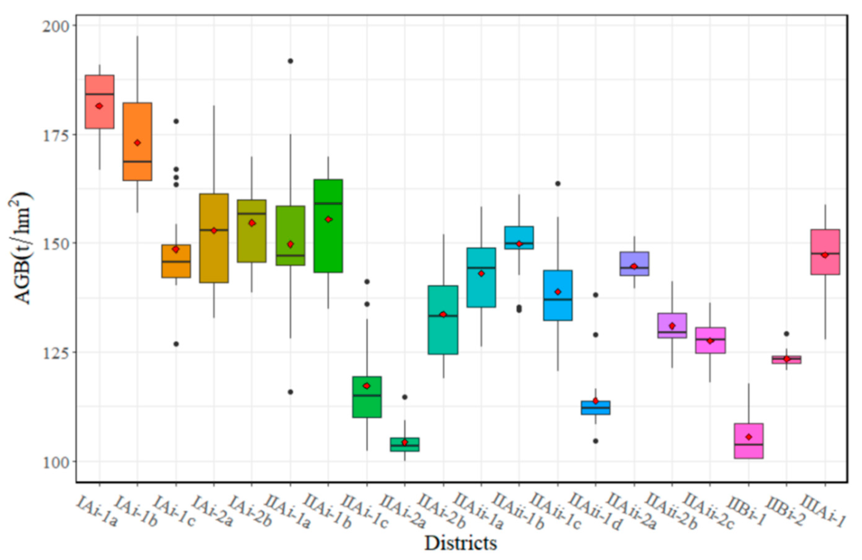
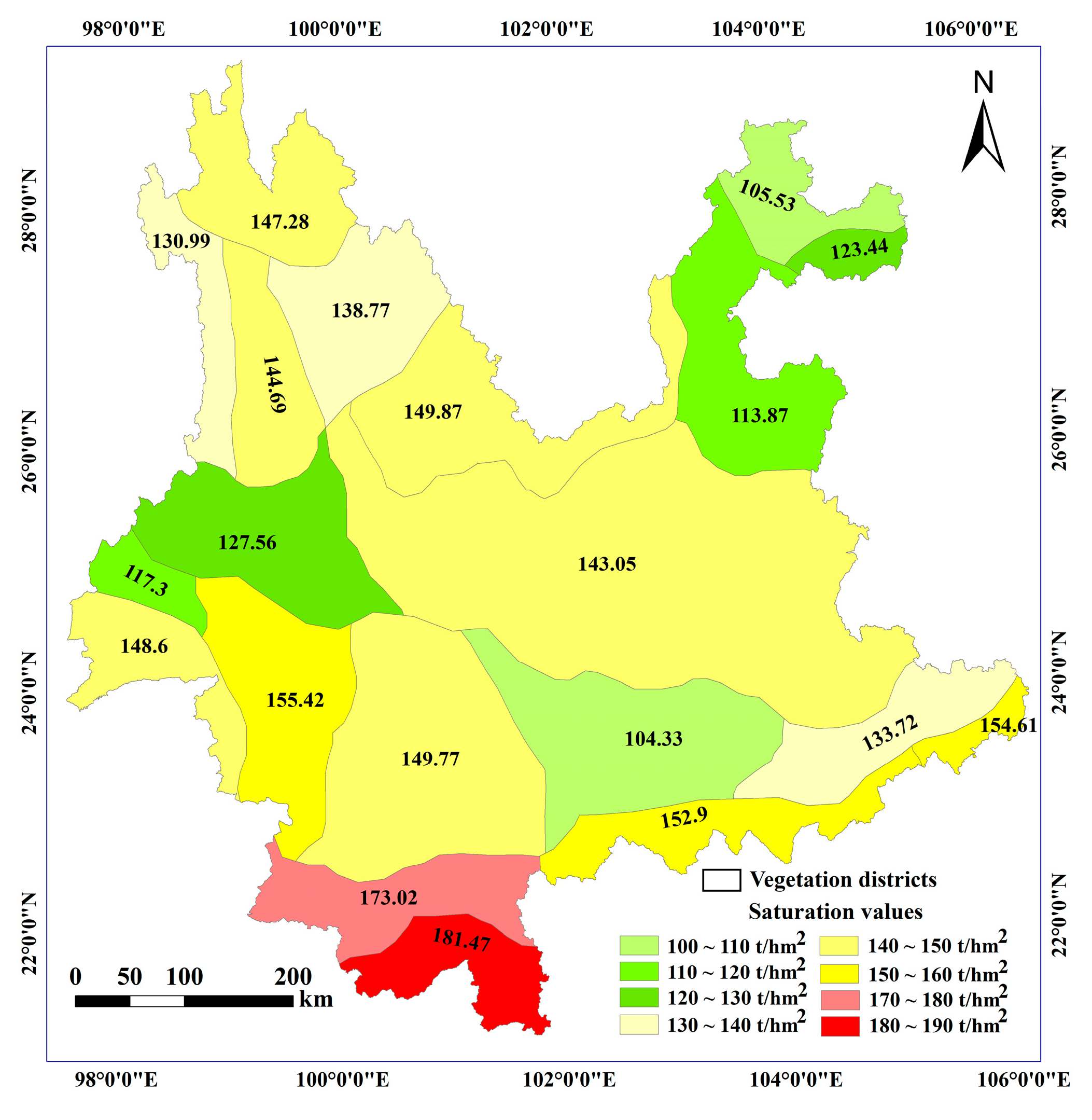
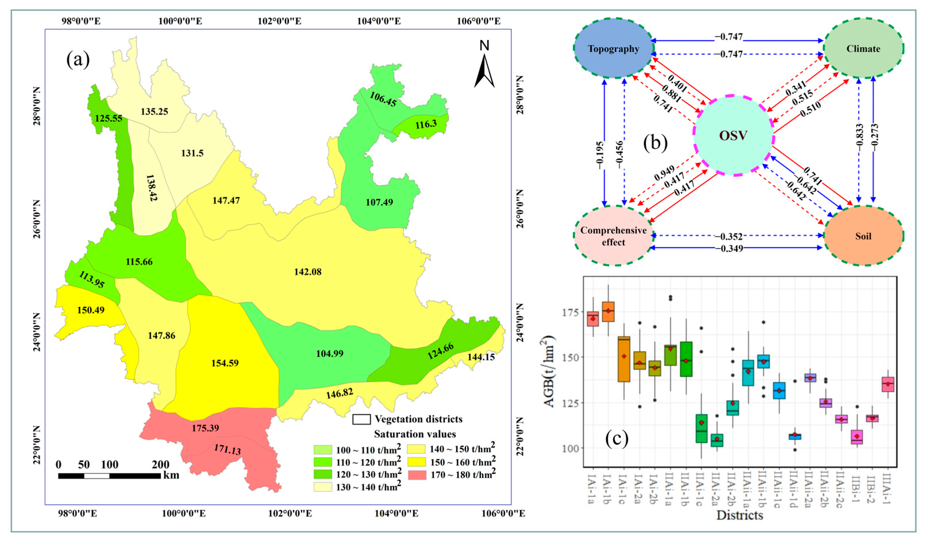
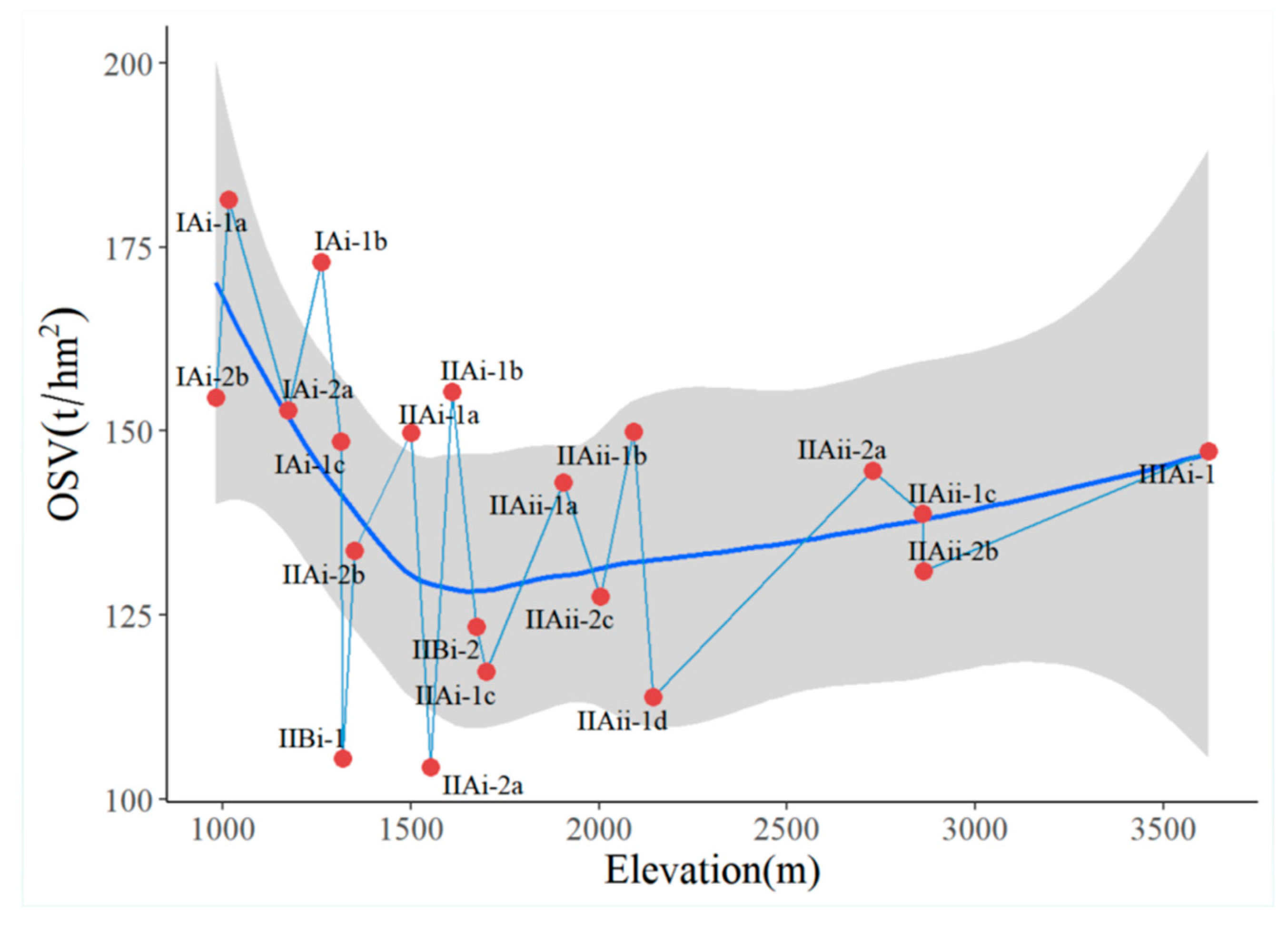
- The red band was used to calculate the OSVs because it had a stronger correlation with oak forest AGBs. The range of OSVs was from 104 t/hm2 to 182 t/hm2. The OSVs were lower in northeastern and western Yunnan, and the highest OSVs were in southern Yunnan.
- (2)
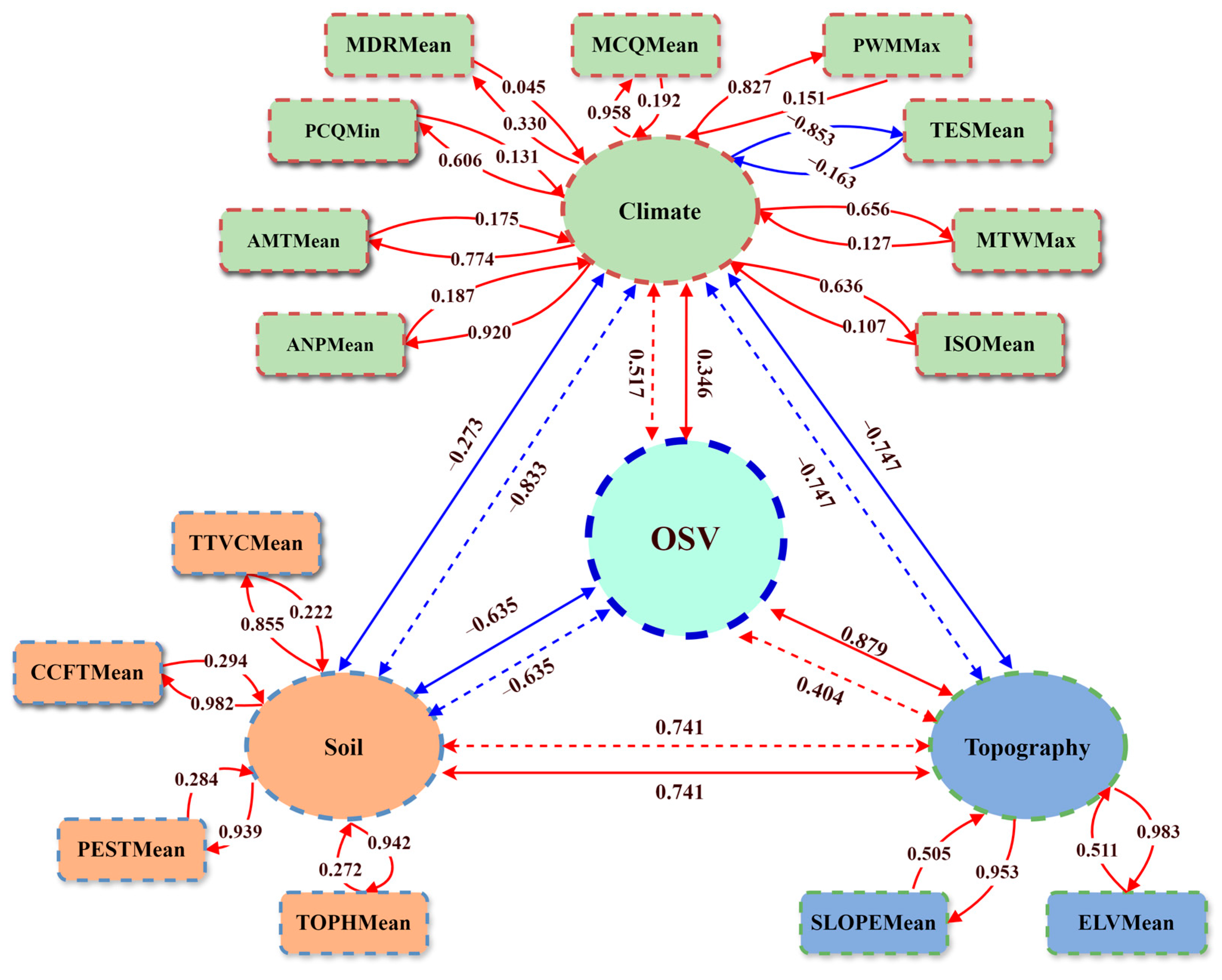
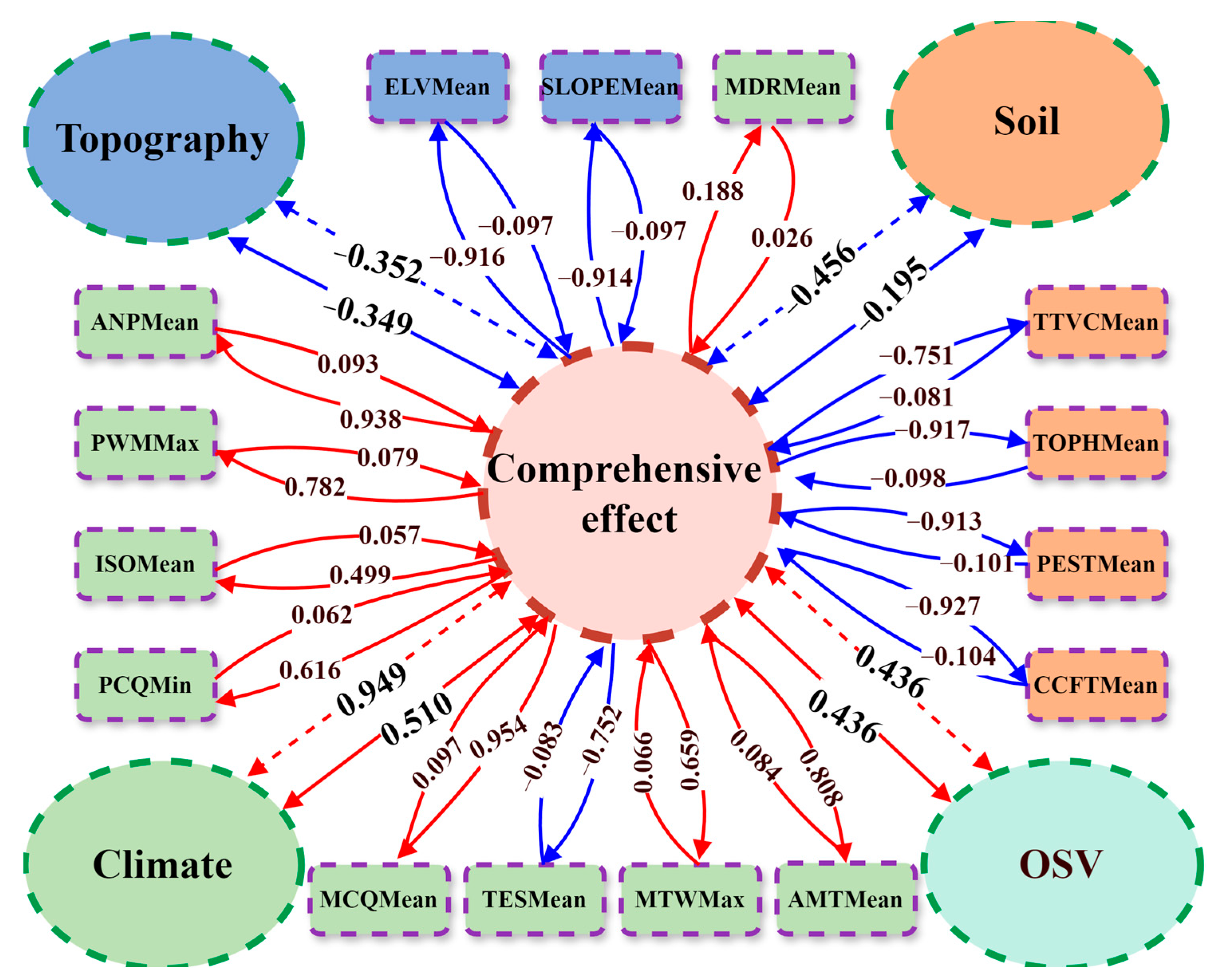
- In the individual effect analysis, the soil factor had the greatest individual effect on the OSV variation, with a correlation coefficient of −0.635, followed by the climate factor at 0.517 and the topography factor at 0.404.
- (3)
- There was a strong interaction effect among the three environmental factors, and the absolute value of the correlation coefficients exceeded 0.7. The interactive effects can affect forest stand structures, leading to variations in the OSVs.
- (4)
- It was evident that the three environmental factors had a strong comprehensive effect (0.436) on the OSVs. The climate factor had the highest effect (0.414) on the OSVs, followed by the soil factor (−0.199) and the topography factor (−0.153). The MCQMean variable showed the highest comprehensive correlation (0.416) with the OSVs.
Author Contributions
Funding
Data Availability Statement
Acknowledgments
Conflicts of Interest
References
- Chen, G.; Zhang, X.; Liu, C.; Liu, C.; Xu, H.; Ou, G. Error Analysis on the Five Stand Biomass Growth Estimation Methods for a Sub-Alpine Natural Pine Forest in Yunnan, Southwestern China. Forests 2022, 13, 1637. [Google Scholar] [CrossRef]
- Lu, D.; Chen, Q.; Wang, G.; Liu, L.; Li, G.; Moran, E. A survey of remote sensing-based aboveground biomass estimation methods in forest ecosystems. Int. J. Digit. Earth 2016, 9, 63–105. [Google Scholar] [CrossRef]
- Hu, T.; Zhang, Y.; Su, Y.; Zheng, Y.; Lin, G.; Guo, Q. Mapping the global mangrove forest aboveground biomass using multisource remote sensing data. Remote Sens. 2020, 12, 1690. [Google Scholar] [CrossRef]
- Zhou, F.; Zhong, D. Kalman filter method for generating time-series synthetic Landsat images and their uncertainty from Landsat and MODIS observations. Remote Sens. Environ. 2020, 239, 111628. [Google Scholar] [CrossRef]
- Zolkos, S.G.; Goetz, S.J.; Dubayah, R. A meta-analysis of terrestrial aboveground biomass estimation using lidar remote sensing. Remote Sens. Environ. 2013, 128, 289–298. [Google Scholar] [CrossRef]
- Chen, Q.; McRoberts, R.E.; Wang, C.; Radtke, P.J. Forest aboveground biomass mapping and estimation across multiple spatial scales using model-based inference. Remote Sens. Environ. 2016, 184, 350–360. [Google Scholar] [CrossRef]
- Wu, Y.; Ou, G.; Lu, T.; Huang, T.; Zhang, X.; Liu, Z.; Yu, Z.; Guo, B.; Wang, E.; Feng, Z.; et al. Improving Aboveground Biomass Estimation in Lowland Tropical Forests across Aspect and Age Stratification: A Case Study in Xishuangbanna. Remote Sens. 2024, 16, 1276. [Google Scholar] [CrossRef]
- Rasshofer, R.H.; Gresser, K. Automotive radar and lidar systems for next generation driver assistance functions. Adv. Radio Sci. 2005, 3, 205–209. [Google Scholar] [CrossRef]
- Urbazaev, M.; Thiel, C.; Cremer, F.; Dubayah, R.; Migliavacca, M.; Reichstein, M.; Schmullius, C. Estimation of forest aboveground biomass and uncertainties by integration of field measurements, airborne LiDAR, and SAR and optical satellite data in Mexico. Carbon Balance Manag. 2018, 13, 5. [Google Scholar] [CrossRef]
- Khanal, S.; Kc, K.; Fulton, J.P.; Shearer, S.; Ozkan, E. Remote sensing in agriculture—Accomplishments, limitations, and opportunities. Remote Sens. 2020, 12, 3783. [Google Scholar] [CrossRef]
- De Sy, V.; Herold, M.; Achard, F.; Asner, G.P.; Held, A.; Kellndorfer, J.; Verbesselt, J. Synergies of multiple remote sensing data sources for REDD+ monitoring. Curr. Opin. Environ. Sustain. 2012, 4, 696–706. [Google Scholar] [CrossRef]
- Gao, Y.; Lu, D.; Li, G.; Wang, G.; Chen, Q.; Liu, L.; Li, D. Comparative analysis of modeling algorithms for forest aboveground biomass estimation in a subtropical region. Remote Sens. 2018, 10, 627. [Google Scholar] [CrossRef]
- Puliti, S.; Breidenbach, J.; Schumacher, J.; Hauglin, M.; Klingenberg, T.F.; Astrup, R. Above-ground biomass change estimation using national forest inventory data with Sentinel-2 and Landsat. Remote Sens. Environ. 2021, 265, 112644. [Google Scholar] [CrossRef]
- López-Serrano, P.M.; Cárdenas Domínguez, J.L.; Corral-Rivas, J.J.; Jiménez, E.; López-Sánchez, C.A.; Vega-Nieva, D.J. Modeling of aboveground biomass with Landsat 8 OLI and machine learning in temperate forests. Forests 2019, 11, 11. [Google Scholar] [CrossRef]
- Huang, T.; Ou, G.; Wu, Y.; Zhang, X.; Liu, Z.; Xu, H.; Xu, X.; Wang, Z.; Xu, C. Estimating the Aboveground Biomass of Various Forest Types with High Heterogeneity at the Provincial Scale Based on Multi-Source Data. Remote Sens. 2023, 15, 3550. [Google Scholar] [CrossRef]
- Imran, A.; Ahmed, S. Potential of Landsat-8 spectral indices to estimate forest biomass. Int. J. Hum. Cap. Urban Manag. 2018, 3, 303. [Google Scholar]
- Li, C.; Li, Y.; Li, M. Improving forest aboveground biomass (AGB) estimation by incorporating crown density and using landsat 8 OLI images of a subtropical forest in Western Hunan in Central China. Forests 2019, 10, 104. [Google Scholar] [CrossRef]
- Tian, L.; Wu, X.; Tao, Y.; Li, M.; Qian, C.; Liao, L.; Fu, W. Review of remote sensing-based methods for forest aboveground biomass estimation: Progress, challenges, and prospects. Forests 2023, 14, 1086. [Google Scholar] [CrossRef]
- Mutanga, O.; Masenyama, A.; Sibanda, M. Spectral saturation in the remote sensing of high-density vegetation traits: A systematic review of progress, challenges, and prospects. ISPRS J. Photogramm. Remote Sens. 2023, 198, 297–309. [Google Scholar] [CrossRef]
- Zhao, P.; Lu, D.; Wang, G.; Wu, C.; Huang, Y.; Yu, S. Examining spectral reflectance saturation in Landsat imagery and cor-responding solutions to improve forest aboveground biomass estimation. Remote Sens. 2016, 8, 469. [Google Scholar] [CrossRef]
- Ou, G.; Lv, Y.; Xu, H.; Wang, G. Improving forest aboveground biomass estimation of Pinus densata forest in Yunnan of Southwest China by spatial regression using Landsat 8 images. Remote Sens. 2019, 11, 2750. [Google Scholar] [CrossRef]
- Gleason, C.J.; Im, J. A review of remote sensing of forest biomass and biofuel: Options for small-area applications. GIScience Remote Sens. 2011, 48, 141–170. [Google Scholar] [CrossRef]
- Zhang, J.; Zhengjun, L.; Xiaoxia, S. Changing landscape in the Three Gorges Reservoir Area of Yangtze River from 1977 to 2005: Land use/land cover, vegetation cover changes estimated using multi-source satellite data. Int. J. Appl. Earth Obs. Geoinf. 2009, 11, 403–412. [Google Scholar] [CrossRef]
- Steininger, M. Satellite estimation of tropical secondary forest above-ground biomass: Data from Brazil and Bolivia. Int. J. Remote Sens. 2000, 21, 1139–1157. [Google Scholar] [CrossRef]
- Zhu, X.; Liu, D. Improving forest aboveground biomass estimation using seasonal Landsat NDVI time-series. ISPRS J. Photogramm. Remote Sens. 2015, 102, 222–231. [Google Scholar] [CrossRef]
- Chen, Y.; Li, L.; Lu, D.; Li, D. Exploring bamboo forest aboveground biomass estimation using Sentinel-2 data. Remote Sens. 2018, 11, 7. [Google Scholar] [CrossRef]
- Jha, N.; Tripathi, N.K.; Barbier, N.; Virdis, S.G.; Chanthorn, W.; Viennois, G.; Brockelman, W.Y.; Nathalang, A.; Tongsima, S.; Sasaki, N. The real potential of current passive satellite data to map aboveground biomass in tropical forests. Remote Sens. Ecol. Conserv. 2021, 7, 504–520. [Google Scholar] [CrossRef]
- Kasischke, E.S.; Melack, J.M.; Dobson, M.C. The use of imaging radars for ecological applications—A review. Remote Sens. Environ. 1997, 59, 141–156. [Google Scholar] [CrossRef]
- Kaufman, Y.J.; Tanre, D. Strategy for direct and indirect methods for correcting the aerosol effect on remote sensing: From AVHRR to EOS-MODIS. Remote Sens. Environ. 1996, 55, 65–79. [Google Scholar] [CrossRef]
- Kolb, A.; Diekmann, M. Effects of environment, habitat configuration and forest continuity on the distribution of forest plant species. J. Veg. Sci. 2004, 15, 199–208. [Google Scholar] [CrossRef]
- Duivenvoorden, J.E. Tree species composition and rain forest-environment relationships in the middle Caquetá area, Colombia, NW Amazonia. Vegetatio 1995, 120, 91–113. [Google Scholar] [CrossRef]
- Moore, I.D.; Norton, T.; Williams, J.E. Modelling environmental heterogeneity in forested landscapes. J. Hydrol. 1993, 150, 717–747. [Google Scholar] [CrossRef]
- Xia, K.; Daws, M.I.; Peng, L.L. Climate drives patterns of seed traits in Quercus species across China. New Phytol. 2022, 234, 1629–1638. [Google Scholar] [CrossRef] [PubMed]
- Asner, G.P.; Flint Hughes, R.; Varga, T.A.; Knapp, D.E.; Kennedy-Bowdoin, T. Environmental and biotic controls over aboveground biomass throughout a tropical rain forest. Ecosystems 2009, 12, 261–278. [Google Scholar] [CrossRef]
- Theissen, T.; Otte, A.; Waldhardt, R. High-mountain landscape classification to analyze patterns of land use and potential natural vegetation. Land 2022, 11, 1085. [Google Scholar] [CrossRef]
- Lamsal, P.; Kumar, L.; Aryal, A.; Atreya, K. Invasive alien plant species dynamics in the Himalayan region under climate change. Ambio 2018, 47, 697–710. [Google Scholar] [CrossRef]
- Yang, Y.; Tian, K.; Hao, J.; Pei, S.; Yang, Y. Biodiversity and biodiversity conservation in Yunnan, China. Biodivers. Conserv. 2004, 13, 813–826. [Google Scholar] [CrossRef]
- Fan, Z.-X.; Thomas, A. Spatiotemporal variability of reference evapotranspiration and its contributing climatic factors in Yunnan Province, SW China, 1961–2004. Clim. Chang. 2013, 116, 309–325. [Google Scholar] [CrossRef]
- Wu, Z.; Zhu, Y. The Vegetation of Yunnan; Science Press: Beijing, China, 1987. [Google Scholar]
- Singh, J.; Rawat, Y.; Chaturvedi, O. Replacement of oak forest with pine in the Himalaya affects the nitrogen cycle. Nature 1984, 311, 54–56. [Google Scholar] [CrossRef]
- Xiao, X.; Haberle, S.G.; Shen, J.; Yang, X.; Han, Y.; Zhang, E.; Wang, S. Latest Pleistocene and Holocene vegetation and climate history inferred from an alpine lacustrine record, northwestern Yunnan Province, southwestern China. Quat. Sci. Rev. 2014, 86, 35–48. [Google Scholar] [CrossRef]
- Xu, J.; Jiang, H. Forests of Yunnan; Yunnan Science and Technology Press: Kunming, China, 1988. [Google Scholar]
- Xu, H.; Zhang, Z.; Ou, G.; Shi, H. A Study on Estimation and Distribution for Forest Biomass and Carbon Storage in Yunnan Province; Yunnan Science and Technology Press: Kunming, China, 2019. [Google Scholar]
- Liu, J.; Weng, F.; Li, Z.; Cribb, M.C. Hourly PM2. 5 estimates from a geostationary satellite based on an ensemble learning algorithm and their spatiotemporal patterns over central east China. Remote Sens. 2019, 11, 2120. [Google Scholar] [CrossRef]
- Wen, L.; Li, Z. Driving forces of national and regional CO2 emissions in China combined IPAT-E and PLS-SEM model. Sci. Total Environ. 2019, 690, 237–247. [Google Scholar] [CrossRef]
- Wang, S.; Li, R.; Wu, Y.; Wang, W. Estimation of surface soil moisture by combining a structural equation model and an artificial neural network (SEM-ANN). Sci. Total Environ. 2023, 876, 162558. [Google Scholar] [CrossRef] [PubMed]
- Moradi, F.; Darvishsefat, A.A.; Pourrahmati, M.R.; Deljouei, A.; Borz, S.A. Estimating aboveground biomass in dense Hyrcanian forests by the use of Sentinel-2 data. Forests 2022, 13, 104. [Google Scholar] [CrossRef]
- Celleri, C.; Zapperi, G.; González Trilla, G.; Pratolongo, P. Assessing the capability of broadband indices derived from Landsat 8 Operational Land Imager to monitor above ground biomass and salinity in semiarid saline environments of the Bahía Blanca Estuary, Argentina. Int. J. Remote Sens. 2019, 40, 4817–4838. [Google Scholar] [CrossRef]
- Muñoz-Huerta, R.F.; Guevara-Gonzalez, R.G.; Contreras-Medina, L.M.; Torres-Pacheco, I.; Prado-Olivarez, J.; Ocampo-Velazquez, R.V. A review of methods for sensing the nitrogen status in plants: Advantages, disadvantages and recent advances. Sensors 2013, 13, 10823–10843. [Google Scholar] [CrossRef]
- Wang, J.; Ding, J.; Yu, D.; Ma, X.; Zhang, Z.; Ge, X.; Teng, D.; Li, X.; Liang, J.; Lizaga, I. Capability of Sentinel-2 MSI data for monitoring and mapping of soil salinity in dry and wet seasons in the Ebinur Lake region, Xinjiang, China. Geoderma 2019, 353, 172–187. [Google Scholar] [CrossRef]
- Fu, B.; Liu, S.; Ma, K.; Zhu, Y. Relationships between soil characteristics, topography and plant diversity in a heterogeneous deciduous broad-leaved forest near Beijing, China. Plant Soil 2004, 261, 47–54. [Google Scholar] [CrossRef]
- Glaser, B.; Lehmann, J.; Zech, W. Ameliorating physical and chemical properties of highly weathered soils in the tropics with charcoal—A review. Biol. Fertil. Soils 2002, 35, 219–230. [Google Scholar] [CrossRef]
- Cailleret, M.; Heurich, M.; Bugmann, H. Reduction in browsing intensity may not compensate climate change effects on tree species composition in the Bavarian Forest National Park. For. Ecol. Manag. 2014, 328, 179–192. [Google Scholar] [CrossRef]
- Macek, M.; Kopecký, M.; Wild, J. Maximum air temperature controlled by landscape topography affects plant species composition in temperate forests. Landsc. Ecol. 2019, 34, 2541–2556. [Google Scholar] [CrossRef]
- Schlesinger, W.H.; Dietze, M.C.; Jackson, R.B.; Phillips, R.P.; Rhoades, C.C.; Rustad, L.E.; Vose, J.M. Forest biogeochemistry in response to drought. Glob. Chang. Biol. 2016, 22, 2318–2328. [Google Scholar] [CrossRef] [PubMed]
- Hoylman, Z.H.; Jencso, K.G.; Hu, J.; Holden, Z.A.; Martin, J.T.; Gardner, W.P. The climatic water balance and topography control spatial patterns of atmospheric demand, soil moisture, and shallow subsurface flow. Water Resour. Res. 2019, 55, 2370–2389. [Google Scholar] [CrossRef]
- Thomas, G.; Dalal, R.; Standley, J. No-till effects on organic matter, pH, cation exchange capacity and nutrient distribution in a Luvisol in the semi-arid subtropics. Soil Tillage Res. 2007, 94, 295–304. [Google Scholar] [CrossRef]
- Lützow, M.V.; Kögel-Knabner, I.; Ekschmitt, K.; Matzner, E.; Guggenberger, G.; Marschner, B.; Flessa, H. Stabilization of organic matter in temperate soils: Mechanisms and their relevance under different soil conditions—A review. Eur. J. Soil Sci. 2006, 57, 426–445. [Google Scholar] [CrossRef]
- Ross, D.; Matschonat, G.; Skyllberg, U. Cation exchange in forest soils: The need for a new perspective. Eur. J. Soil Sci. 2008, 59, 1141–1159. [Google Scholar] [CrossRef]
- Sharma, A.; Weindorf, D.C.; Wang, D.; Chakraborty, S. Characterizing soils via portable X-ray fluorescence spectrometer: 4. Cation exchange capacity (CEC). Geoderma 2015, 239, 130–134. [Google Scholar] [CrossRef]
- Smith, P. Soils and climate change. Curr. Opin. Environ. Sustain. 2012, 4, 539–544. [Google Scholar] [CrossRef]
- Certini, G.; Scalenghe, R. The crucial interactions between climate and soil. Sci. Total Environ. 2023, 856, 159169. [Google Scholar] [CrossRef]
- Ravi, S.; Breshears, D.D.; Huxman, T.E.; D’Odorico, P. Land degradation in drylands: Interactions among hydrologic–aeolian erosion and vegetation dynamics. Geomorphology 2010, 116, 236–245. [Google Scholar] [CrossRef]
- Corwin, D.L. Climate change impacts on soil salinity in agricultural areas. Eur. J. Soil Sci. 2021, 72, 842–862. [Google Scholar] [CrossRef]
- Dillon, G.K.; Holden, Z.A.; Morgan, P.; Crimmins, M.A.; Heyerdahl, E.K.; Luce, C.H. Both topography and climate affected forest and woodland burn severity in two regions of the western US, 1984 to 2006. Ecosphere 2011, 2, 1–33. [Google Scholar] [CrossRef]
- Sobek, S.; Tranvik, L.J.; Prairie, Y.T.; Kortelainen, P.; Cole, J.J. Patterns and regulation of dissolved organic carbon: An analysis of 7,500 widely distributed lakes. Limnol. Oceanogr. 2007, 52, 1208–1219. [Google Scholar] [CrossRef]
- Zhou, Y.; Yi, Y.; Liu, H.; Song, J.; Jia, W.; Zhang, S. Altitudinal trends in climate change result in radial growth variation of Pinus yunnanensis at an arid-hot valley of southwest China. Dendrochronologia 2022, 71, 125914. [Google Scholar] [CrossRef]
- Xu, Z.; Zhao, B.; Wang, Y.; Xiao, J.; Wang, X. Composting process and odor emission varied in windrow and trough composting system under different air humidity conditions. Bioresour. Technol. 2020, 297, 122482. [Google Scholar] [CrossRef]
- Keitt, T.H.; Bjørnstad, O.N.; Dixon, P.M.; Citron-Pousty, S. Accounting for spatial pattern when modeling organism-environment interactions. Ecography 2002, 25, 616–625. [Google Scholar] [CrossRef]
- Trenberth, K.E. Changes in precipitation with climate change. Clim. Res. 2011, 47, 123–138. [Google Scholar] [CrossRef]
- Moser, G.; Leuschner, C.; Hertel, D.; Graefe, S.; Soethe, N.; Iost, S. Elevation effects on the carbon budget of tropical mountain forests (S Ecuador): The role of the belowground compartment. Glob. Chang. Biol. 2011, 17, 2211–2226. [Google Scholar] [CrossRef]
- Körner, C. The use of ‘altitude’in ecological research. Trends Ecol. Evol. 2007, 22, 569–574. [Google Scholar] [CrossRef]
- Obanor, F.O.; Walter, M.; Jones, E.E.; Jaspers, M.V. Effect of temperature, relative humidity, leaf wetness and leaf age on Spilocaea oleagina conidium germination on olive leaves. Eur. J. Plant Pathol. 2008, 120, 211–222. [Google Scholar] [CrossRef]
- Sheil, D.; Murdiyarso, D. How forests attract rain: An examination of a new hypothesis. Bioscience 2009, 59, 341–347. [Google Scholar] [CrossRef]
- Price, K. Effects of watershed topography, soils, land use, and climate on baseflow hydrology in humid regions: A review. Prog. Phys. Geogr. 2011, 35, 465–492. [Google Scholar] [CrossRef]
- Unger, M.; Homeier, J.; Leuschner, C. Effects of soil chemistry on tropical forest biomass and productivity at different elevations in the equatorial Andes. Oecologia 2012, 170, 263–274. [Google Scholar] [CrossRef]
- Knipling, E.B. Physical and physiological basis for the reflectance of visible and near-infrared radiation from vegetation. Remote Sens. Environ. 1970, 1, 155–159. [Google Scholar] [CrossRef]
- Gilgen, A.K.; Buchmann, N. Response of temperate grasslands at different altitudes to simulated summer drought differed but scaled with annual precipitation. Biogeosciences 2009, 6, 2525–2539. [Google Scholar] [CrossRef]
- Chen, F.; Fan, Z.; Niu, S.; Zheng, J. The influence of precipitation and consecutive dry days on burned areas in Yunnan Province, Southwestern China. Adv. Meteorol. 2014, 2014, 748923. [Google Scholar] [CrossRef]
- Hernández-Stefanoni, J.L.; Castillo-Santiago, M.Á.; Mas, J.F.; Wheeler, C.E.; Andres-Mauricio, J.; Tun-Dzul, F.; George-Chacón, S.P.; Reyes-Palomeque, G.; Castellanos-Basto, B.; Vaca, R. Improving aboveground biomass maps of tropical dry forests by integrating LiDAR, ALOS PALSAR, climate and field data. Carbon Balance Manag. 2020, 15, 15. [Google Scholar] [CrossRef]
- Fu, L.; Lei, X.; Hu, Z.; Zeng, W.; Tang, S.; Marshall, P.; Cao, L.; Song, X.; Yu, L.; Liang, J. Integrating regional climate change into allometric equations for estimating tree aboveground biomass of Masson pine in China. Ann. For. Sci. 2017, 74, 42. [Google Scholar] [CrossRef]
- Shao, G.; Shao, G.; Gallion, J.; Saunders, M.R.; Frankenberger, J.R.; Fei, S. Improving Lidar-based aboveground biomass estimation of temperate hardwood forests with varying site productivity. Remote Sens. Environ. 2018, 204, 872–882. [Google Scholar] [CrossRef]
- Zhou, J.-J.; Zhao, Z.; Zhao, Q.; Zhao, J.; Wang, H. Quantification of aboveground forest biomass using Quickbird imagery, topographic variables, and field data. J. Appl. Remote Sens. 2013, 7, 073484. [Google Scholar] [CrossRef]
- Su, Y.; Guo, Q.; Xue, B.; Hu, T.; Alvarez, O.; Tao, S.; Fang, J. Spatial distribution of forest aboveground biomass in China: Estimation through combination of spaceborne lidar, optical imagery, and forest inventory data. Remote Sen. Environ. 2016, 173, 187–199. [Google Scholar] [CrossRef]


| Regions | Subregions | Zones | Districts or Subdistricts |
|---|---|---|---|
| Region of tropical monsoon rainforests and tropical rainforests | Subregion of western (xerophytic) tropical rain forests and monsoon forests | Zone of seasonal rainforests and semi-evergreen seasonal rainforests at the northern margin of the monsoon tropics | Subdistrict of Antiaris toxicaria, Pouteria grandifolia, Canarium subulatum, Ficus altissima, and Chukrasia tabularis forests of the southern midmountain basin of Xishuangbanna (IAi-1a) |
| Subdistrict of Terminalia myriocarpa and Pometia pinnata forests, semecarpus albescens, and Machilus nanmu forests of the northern midmountain basin of Xishuangbanna (IAi-1b) | |||
| Subdistrict of Ficus altissima and Chukrasia tabularis forests of the middle and broad valleys of southwest Yunnan (IAi-1c) | |||
| Subdistrict of Dipterocarpus retusus, Hopea chinensis, Cinnamomum camphora, Camellia sinensis, and Magnolia sp., forests of the Honghe and Wenshan Prefectures, south rim valley (IAi-2a) | |||
| Subdistrict of Lysidce rhodostegia and Ficus altissima forests of the low mountain valleys of southeastern Wenshan Prefecture (IAi-2b) | |||
| Region of subtropical evergreen broad-leaved forests | Subregion of western (semi-humid) evergreen broad-leaved forests | Zone of subtropical monsoon evergreen broad-leaved forests of the southern plateau | Subdistrict of Castanopsis hystrix, Castanopsis orthacantha, and Pinus yunnanensis forests of the midmountain plateau, located in the middle reaches of the Lancang River (IIAi-1a) |
| Subdistrict of Castanopsis hystrix, Castanopsis indica, and Lithocarpuse chinotholus forests of the mountains in Lincang (IIAi-1b) | |||
| Subdistrict of Castanopsis ferox, Castanopsis hystrix, and Lithocarpus truncatus forests of the midmountainous plateaus of Longling and Lianghe (IIAi-1c) | |||
| Subdistrict of Pinus yunnanensis and Schima wallichii forests and Bombax ceiba and Woodfordia fruticosa bushes of the karst plateau valley of Mengzi and Yuanjiang (IIAi-2a) | |||
| Subdistrict of Castanopsis faberi and Castanopsis fissa forests of the Wenshan karst plateau (IIAi-2b) | |||
| Zone of subtropical northern broad-leaved evergreen forests of the plateau | Subdistrict of Quercus glaucoides, Castanopsis orthacantha, and Pinus yunnanensis forests of the basin valley of the central Yunnan plateau (IIAii-1a) | ||
| Subdistrict of Pinus yunnanensis and alpine oak forests in the middle and northern Yunnan mountain valleys (IIAii-1b) | |||
| Subdistrict of Pinus yunnanensis, Picea asperata, and Abies fabri forests of the high mountain plateau of northwestern central Yunnan (IIAii-1c) | |||
| Subdistrict of Leymus chinensis meadows and Pinus yunnanensis forest in the high and middle areas of the northeastern Yunnan plateau (IIAii-1d) | |||
| Subdistrict of Pinus yunnanensis, Castanopsis orthacantha, and Abies fabri forests in the high and middle mountain valleys of the Yunling and Lancang rivers (IIAii-2a) | |||
| Subdistrict of Quercus glauca, Taiwania cryptomerioides, and Neyraudia reynaudiana forests, tall grasses of the high and middle mountain valleys of the Gaoligong Mountain, Nujiang River, and Biluo Snow Mountain (IIAii-2b) | |||
| Subdistrict of Pinus yunnanensis and Tsuga dumosa forests of the midmountain area of western Yunnan (IIAii-2c) | |||
| Subregion of eastern (humid) evergreen broad-leaved forests | Zone of eastern (mid-sub-tropical zone) broad-leaved evergreen forests | District of Castanopsis platyacantha and Lithocarpus cleistocarpus forests along the midmountain valleys of northeastern Yunnan (IIBi-1) | |
| District of Lithocarpus cleistocarpus, Castanopsis platyacantha, and deciduous oak forests in the karst plateau of Zhenxiong (IIBi-2) | |||
| Region of Tibetan Plateau alpine vegetation | Subregion of Montane cold temperate coniferous forests in the southeast of the plateau | Zone of cold temperate coniferous forests and meadows at the south-eastern edge of the Qinghai–Tibet Plateau | District of Picea asperata and Abies fabri forests and kobresia sp., shrub meadows in Deqin and the off-mountain plateau of Zhongdian (IIIAi-1) |
| Forest | Age | BEF | SVD (t/m3) |
|---|---|---|---|
| Oak | Young forest | 1.3798 | 0.6760 |
| Half-mature forest | 1.3947 | ||
| Near-mature forest | 1.2517 | ||
| Mature forest | 1.1087 | ||
| Over-mature forest | 1.1802 |
| No. | Image ID | Acquisition Date | Solar Elevation (°) | Solar Azimuth (°) | Mean Cloud Cover (%) |
|---|---|---|---|---|---|
| 1 | LC81330402016307LGN00 | 2 November 2016 | 42.8681 | 155.7033 | 1.56 |
| 2 | LC81330412016323LGN00 | 18 November 2016 | 39.8182 | 156.6044 | 0.89 |
| 3 | LC81320402016348LGN00 | 13 December 2016 | 34.2199 | 156.6774 | 0.73 |
| 4 | LC81320412016348LGN00 | 13 December 2016 | 34.4429 | 156.0007 | 0.76 |
| 5 | LC81320422016348LGN00 | 13 December 2016 | 36.6581 | 155.2988 | 0.32 |
| 6 | LC81320432016012LGN02 | 12 January 2016 | 37.6659 | 150.1239 | 3.68 |
| 7 | LC81300442016046LGN00 | 15 February 2016 | 45.3711 | 141.0448 | 0.01 |
| 8 | LC81310412016325LGN01 | 20 November 2016 | 39.3429 | 156.6972 | 0.52 |
| 9 | LC81310422016005LGN02 | 5 January 2016 | 36.0148 | 152.2167 | 0.05 |
| 10 | LC81310432016325LGN01 | 20 November 2016 | 41.7926 | 155.1058 | 0.99 |
| 11 | LC81310442016325LGN01 | 20 November 2016 | 42.9976 | 154.2569 | 4.57 |
| 12 | LC81310452016069LGN00 | 9 March 2016 | 53.3872 | 132.1974 | 0.10 |
| 13 | LC81300412016030LGN00 | 30 January 2016 | 38.2410 | 148.0217 | 1.28 |
| 14 | LC81300422016030LGN01 | 30 January 2016 | 39.3315 | 147.1280 | 0.24 |
| 15 | LC81300432016046LGN00 | 15 February 2016 | 44.3817 | 142.2120 | 2.22 |
| 16 | LC81300442016046LGN00 | 15 February 2016 | 45.3711 | 141.0448 | 0.01 |
| 17 | LC81300452016046LGN00 | 15 February 2016 | 46.3395 | 139.8293 | 0.01 |
| 18 | LC81290402016151LGN00 | 30 May 2016 | 65.6228 | 119.6986 | 13.92 |
| 19 | LC81290412016343LGN00 | 8 December 2016 | 36.0345 | 156.3999 | 2.22 |
| 20 | LC81290422016327LGN00 | 22 November 2016 | 40.1300 | 155.9964 | 0.79 |
| 21 | LC81290432016327LGN00 | 22 November 2016 | 41.3464 | 155.1964 | 0.15 |
| 22 | LC81290442016039LGN00 | 8 February 2016 | 43.5143 | 142.9442 | 5.92 |
| 23 | LC81290452016119LGN00 | 28 April 2016 | 66.7992 | 104.7207 | 1.22 |
| 24 | LC81280412016208LGN00 | 26 July 2016 | 66.3707 | 104.7760 | 5.18 |
| 25 | LC81280422016080LGN01 | 20 March 2016 | 54.6560 | 133.4815 | 4.31 |
| 26 | LC81280432016128LGN00 | 7 May 2016 | 67.7248 | 105.7585 | 1.41 |
| 27 | LC81280442016128LGN00 | 7 May 2016 | 67.8515 | 102.0989 | 13.36 |
| 28 | LC81270432016041LGN00 | 10 February 2016 | 43.0065 | 143.5091 | 4.66 |
| 29 | LC81270442016281LGN00 | 7 October 2016 | 55.0915 | 142.9570 | 4.64 |
| Variables | Description | Variables | Description |
|---|---|---|---|
| AMTMean | The mean of annual mean temperature (°C) | BSTSMean | The mean of base saturation in the topsoil (%) |
| MDRMean | The mean of mean temperature diurnal range (°C) | CCFTMean | The mean of cation exchange capacity of the clay fraction in the topsoil (meq/100 g) |
| ISOMean | The mean of isothermality (%) | CECTMean | The mean of cation exchange capacity in the topsoil (meq/100 g) |
| TESMean | The mean of temperature seasonality (°C) | ESPTMean | The mean of exchangeable sodium percentage in the topsoil (%) |
| MTWMax | The max of maximum temperatures in the warmest month (°C) | PSATMean | The mean percentage of the sand in the topsoil (%) |
| MTCMin | The min of the minimum temperatures in the coldest month (°C) | PESTMean | The mean percentage of the silt in the topsoil (%) |
| TARMean | The mean of temperature annual range (°C) | TTVCMean | The mean of topsoil texture class Variables and code (-) |
| MTQMean | The mean of the mean temperatures in the wettest quarter (°C) | PECTMean | The mean of the percentage of clay in the topsoil (%) |
| MTDMean | The mean of the mean temperatures in the driest quarter (°C) | CCCTMean | The mean of calcium carbonate content in the topsoil (%) |
| MWQMean | The mean temperature in the warmest quarter (°C) | TRBDMean | The mean of topsoil reference bulk density (g/cm³) |
| MCQMean | The mean of the mean temperatures in the coldest quarter (°C) | ELCTMean | The mean of electrical conductivity of the topsoil (S/m) |
| ANPMean | The mean of annual precipitation (mm) | VPGTMean | The mean volume percentage of the gravel in the topsoil (%) |
| PWMMax | The max of precipitation in the wettest month (mm) | POCTMean | The mean of the percentage of organic carbon in the topsoil (%) |
| PDMMin | The min of precipitation in the driest month (mm) | TOPHMean | The mean of topsoil pH (-) |
| PRSMean | The mean of precipitation seasonality (mm) | TEBTMean | The mean of total exchangeable bases in the topsoil (meq/100 g) |
| PRWMax | The max of precipitation in the wettest quarter (mm) | ELVMean | The mean elevation (m) |
| PRDMin | The min of precipitation in the driest quarter (mm) | SLOPEMean | The mean of the slope (-) |
| PWQMax | The max of precipitation in the warmest quarter (mm) | ASPECTMean | The mean of the aspect (°) |
| PCQMin | The min of precipitation in the coldest quarter (mm) |
| Variables | Types | Size | R2 | AVE | GFI | RMSEA |
|---|---|---|---|---|---|---|
| Climate | Exogenous | 9 | 0.000 | 0.565 | 0.909 | 0.045 |
| Topography | Endogenous | 2 | 0.560 | 0.985 | ||
| Soil | Endogenous | 4 | 0.940 | 0.866 | ||
| OSVs | Endogenous | 1 | 0.367 | 1.000 | ||
| Environment | Endogenous | 15 | 1.000 | 0.625 |
Disclaimer/Publisher’s Note: The statements, opinions and data contained in all publications are solely those of the individual author(s) and contributor(s) and not of MDPI and/or the editor(s). MDPI and/or the editor(s) disclaim responsibility for any injury to people or property resulting from any ideas, methods, instructions or products referred to in the content. |
© 2024 by the authors. Licensee MDPI, Basel, Switzerland. This article is an open access article distributed under the terms and conditions of the Creative Commons Attribution (CC BY) license (https://creativecommons.org/licenses/by/4.0/).
Share and Cite
Wu, Y.; Ou, G.; Huang, T.; Zhang, X.; Liu, C.; Liu, Z.; Yu, Z.; Luo, H.; Lu, C.; Shi, K.; et al. Climate Interprets Saturation Value Variations Better Than Soil and Topography in Estimating Oak Forest Aboveground Biomass Using Landsat 8 OLI Imagery. Remote Sens. 2024, 16, 1338. https://doi.org/10.3390/rs16081338
Wu Y, Ou G, Huang T, Zhang X, Liu C, Liu Z, Yu Z, Luo H, Lu C, Shi K, et al. Climate Interprets Saturation Value Variations Better Than Soil and Topography in Estimating Oak Forest Aboveground Biomass Using Landsat 8 OLI Imagery. Remote Sensing. 2024; 16(8):1338. https://doi.org/10.3390/rs16081338
Chicago/Turabian StyleWu, Yong, Guanglong Ou, Tianbao Huang, Xiaoli Zhang, Chunxiao Liu, Zhi Liu, Zhibo Yu, Hongbin Luo, Chi Lu, Kaize Shi, and et al. 2024. "Climate Interprets Saturation Value Variations Better Than Soil and Topography in Estimating Oak Forest Aboveground Biomass Using Landsat 8 OLI Imagery" Remote Sensing 16, no. 8: 1338. https://doi.org/10.3390/rs16081338