1. Introduction
In recent years, wind lidar profilers have gained prominence as the preferred measurement technology, gradually replacing traditional meteorological masts equipped with in-situ sensors like anemometers. They demonstrate proficiency in capturing mean wind profiles, providing data quality comparable to fixed masts, all while allowing for measurements at the same or even greater heights above the water surface. Studies conducted during the 2000s underscored the effectiveness of wind lidar technology in wind speed measurement, evidenced by comparisons with anemometry data obtained from met masts [
1,
2]. Additionally, Ref. [
3] utilized wind lidar profilers to evaluate vertical shear and wind profiles, revealing an overestimation of kinetic energy flux in vertical shear, directly impacting wind turbine power curves. Recognizing the necessity of measuring wind speed and direction at various altitudes, Ref. [
4] advocated for the utilization of wind lidar profilers, proposing a validated procedure compared against met mast anemometers. Moreover, Ref. [
5] demonstrated the efficacy of wind lidar profilers in conducting site-specific wind resource assessments, affirming their value as a vital tool in the field.
For offshore wind resource assessment, lidar systems are deployed on self-contained floating structures, such as buoys, collectively forming what is known as a floating lidar system (FLS). This system provides a cost-effective solution for acquiring essential wind data in offshore environments, as well as certified instruments to provide mean wind statistics such as wind speed and wind direction. However, wind lidar profilers, either ground-based or mounted on a buoy, fall short in accurately characterizing turbulence, i.e., velocity fluctuations. The precise measurement of turbulence is indispensable for establishing characteristic design conditions for wind turbines and plays a pivotal role in developing robust design tools that enhance their survivability, reliability, and performance. Therefore, integrating turbulence measurement capabilities into FLS is an indispensable stride towards realizing these benefits.
Turbulence measurements obtained from lidar profilers are subject to two main systematic errors induced by the intra-beam effect, i.e., the averaging effect of the probe volume and the inter-beam effect, also known as the cross-contamination effect, e.g., [
6,
7]. The intra-beam effect is a consequence of the probe length, effectively acting as a low-pass filter. This phenomenon stems from the "filtering" out of eddies that fall beneath the size threshold set by the probe length, generating underestimation of turbulence metrics. The inter-beam effect can lead to either underestimation or overestimation of turbulence metrics. This discrepancy arises from the modulation of energy associated with eddies characterized by specific wavenumbers.
Another source of error arises when utilizing FLS. Buoys are subject to translational and rotational motions, which can have a detrimental impact on the lidar’s measurements. The motions of the buoy further contribute to introducing high-frequency fluctuations to the recorded wind data. In the past decade, few studies have examined the impact of motion on wind speed, wind direction, and turbulence measurements. Ref. [
8] utilized a software-based motion simulator to replicate the velocity azimuth display of a ZephIR 300 lidar. They employed a moment-computation recursive procedure to estimate the motion-induced error standard deviation in horizontal wind speed, as well as the motion-induced turbulence intensity (TI), under simple harmonic motion conditions. Additionally, Ref. [
9] employed numerical and analytical methods to quantitatively assess bias in lidar wind speed measurements. Their investigation revealed that bias was influenced by several factors, including amplitude and period of motion, the angle between motion and wind direction, wind speed, and the strength of wind shear. Ref. [
10] utilized simulated lidar profiler measurements within synthetic atmospheric turbulence fields to evaluate how buoy motions affect turbulence estimation. Their simulations revealed that translational motions of the buoy notably influenced the accuracy of turbulence estimates. Furthermore, a recent study by [
11] specifically identified the influence of pitch motion on wind speed measurements acquired through nacelle-based lidar.
An alternative experimental approach for studying the impact of motion involves placing a wind lidar on a moving platform and comparing its measurements with data obtained from a nearby stationary lidar system of the same type or anemometer mounted on a meteorological mast. For instance, Ref. [
12] conducted experimental investigations to analyze the effects of motions originating from a moving platform on WindCube v2 lidar measurements. While the mean wind speed and direction measurements showed little difference compared to fixed reference measurements, TI measured by the mobile lidar was consistently higher. Ref. [
13] conducted a study showcasing their findings utilizing two distinct lidar models (WindCube and ZephIR) across a spectrum of over fifty motion scenarios, revolving around a single axis. However, it is worth noting that their selected motion patterns might not perfectly mirror typical FLS. Furthermore, each scenario, executed only once, spanned a duration of 3 h, posing challenges in drawing definitive conclusions regarding the influence of wind speed on motion-induced errors, given the limited variability observed within the 3 h timeframe. Similarly, Ref. [
14] utilized a ZephIR lidar in various scenarios, albeit for brief time periods, thus providing insights into motion-related errors but with limitations in statistical assessment.
These studies offer valuable insights into the repercussions of motion-induced effects on wind measurements. While their primary focus lies in examining mean wind statistics, they establish a foundational understanding of the factors influencing the accuracy and reliability of lidar-based measurements across diverse motion scenarios. Serving as essential groundwork, these prior investigations illuminate the complexities and challenges inherent in mitigating motion-related errors in lidar-based wind measurements.
Further research endeavors are imperative to conduct experimental testing onshore, employing motion platforms that simulate typical sea motions. Such experiments not only validate previous findings, which have predominantly centered on mean wind statistics, but are also indispensable for delving deeper into the impact of motion on turbulence measurement collected by FLS.
In this study, our objective is to address this research gap by quantifying wind fluctuations measured by a lidar mounted on a moving platform and comparing them to a reference fixed lidar. To recreate potential buoy movements, we employed a hexapod within a controlled environment. Initially, we focused on rotations around a single axis, varying the amplitudes and periods. Subsequently, we explored the impact of coupling two and three rotational degrees of freedom on velocity fluctuations measured by the mobile lidar. The experimental campaign was conducted onshore over several weeks to gather measurements encompassing different wind speed ranges.
Structure of this Work
The structure of this paper is as follows: In
Section 2, we establish the context by elaborating on the data and methodology. This includes insights into our onshore experimental campaign, where a WindCube v2.1 lidar was mounted on a hexapod to simulate buoy-like motion, and a fixed lidar served as a reference. Subsections are utilized to specify motion parameters and assessment criteria aimed at evaluating the influence of crucial factors on turbulence measurement derived from FLS. These factors include motion amplitude, period, wind speed, wind direction, measurement height, and wind shear. In
Section 3.1, we present our findings, encompassing preliminary observations and the impact of the aforementioned factors on turbulent velocity fluctuations measured along the line-of-sight (LOS), as well as in both along-wind and cross-wind directions.
Section 4 delves into in-depth discussions, dissecting the influence of each factor on turbulence measurement obtained by the FLS. Finally, in
Section 5, we underscore the potential advantages of this study in providing precise turbulence data to enhance the optimization of offshore wind farm design and energy production.
2. Data and Method
2.1. Coordinate System
The present study employs the LOS velocities. They represent the speed at which air masses are moving towards or away from the lidar instrument along the line of sight of the laser beam emitted by the lidar. The LOS velocities are combined to calculate the horizontal components (
and
) of the wind speed in the instrument coordinate system defined by the beam directions. This instrument coordinate system matches that of the hexapod wherein the
x component is oriented from beam 4 towards beam 2, the
y component points from beam 3 towards beam 1 and is aligned with the
y-axis of the hexapod (
Figure 1b), and the vertical
z component points upwards along beam 5.
Defining the wind field in the direction of beam
i as
, with positive velocity being towards the instrument, the coordinate transformation from beam coordinates to instrument coordinates is given by Equations (
1) and (
2):
where
= 28° is the zenith angle. To align with the methodology outlined by Kaimal and Finnigan [
15], the coordinate axes were rotated. This adjustment ensured that the
aligned with the 10 min mean wind direction, and the mean velocity of
became 0, thereby yielding the along-wind and cross-wind velocities, referred to as
u and
v, respectively.
2.2. Experimental Campaign
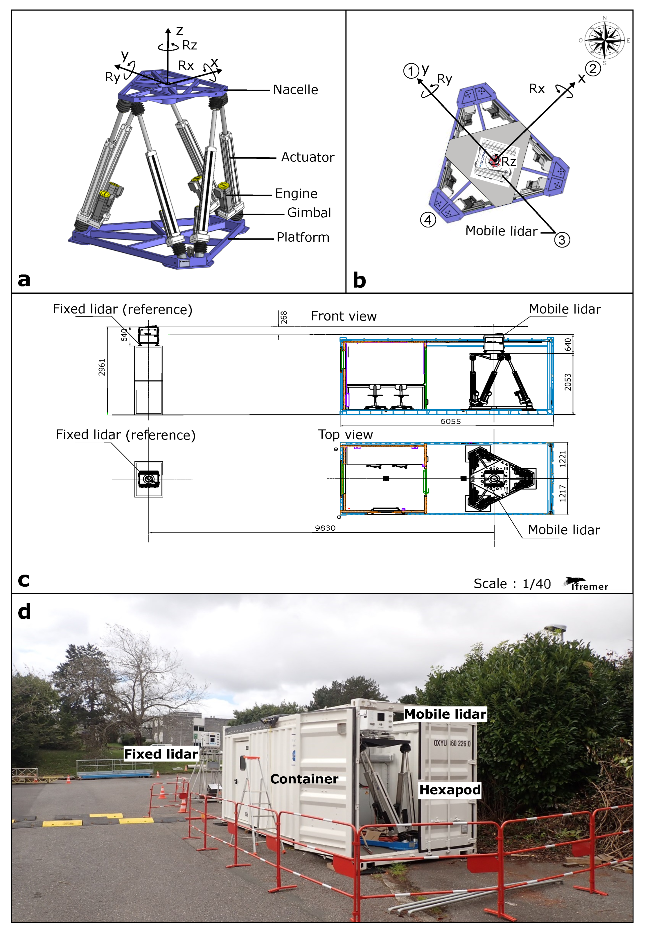
The experimental campaign was conducted at Ifremer’s site in Brest, France. The experimental setup consisted of two WindCube v2.1 lidars deployed onshore. One lidar was installed in a fixed configuration, providing reference measurements, while the second lidar was installed on a Stewart platform, also known as a hexapod. The lidar installed on the hexapod is referred to as the “mobile lidar”. The hexapod used in the experiment is the Mistral 800 by SYMETRIE. It consists of a lower (base) platform and an upper (nacelle) platform that can perform movements along all six degrees of freedom (
Figure 1a). The maximum range of motion and dynamic capabilities of the hexapod are detailed in
Table 1. The hexapod enables a wide range of courses, speeds, and accelerations particularly for rotational motions. Hereafter, rotations around the
x,
y, and
z axes are referred to as Rx, Ry, and Rz, respectively.
The translation motions with the hexapod are severely limited due to the shorter courses enabled by the technology. The approximately one-meter limit on translational motion represents the primary constraint within this experimental setup. It is important to note that offshore buoys encounter diverse conditions, often experiencing movements exceeding this limit due to factors like their specific design, geographical location, and the dynamic forces present in the environment. This limitation in our experiment aims to replicate certain aspects of buoy motion but does not encompass the full range of movements that buoys might encounter in real offshore conditions.
The two lidars were positioned approximately 10 m apart from each other. To ensure their protection, the mobile lidar and the hexapod were housed inside a container (
Figure 1d). The hexapod and its connector are sensitive to humidity and therefore cannot be operated during rainy conditions.
The LOS velocity data from a standard commercial WindCube v2.1 lidar typically operates at a sampling rate of 0.25 Hz. However, for this experiment, a prototype configuration of the lidar, featuring a fourfold increase in sampling rate to 1 Hz, was employed. This improvement was achieved by significantly reducing the accumulation time for data collection from each beam by 70%, in conjunction with a corresponding 70% reduction in the number of transmitted pulses. The zenith angle and probe length of the prototype configuration match the commercial configuration, with the latter being approximately 23 m. Before the deployment detailed in this paper, both lidars underwent an independent performance verification conducted at the DNV Remote Sensing test site in Janneby, Germany, involving comparison against a meteorological mast. The decision to enhance the sampling rate aimed to elevate the accuracy of turbulent fluctuations measurements, expecting to capture smaller eddies and their turbulent energy. A more comprehensive exploration of this research is anticipated to be submitted for publication in the near future.
The inertial unit located on the hexapod had a sampling rate of 100 Hz. For power supply, the lidars were connected to electricity in a building situated approximately 15 m southeast of the working area. Both lidars were installed at a height of 3 m above the ground (
Figure 1c).
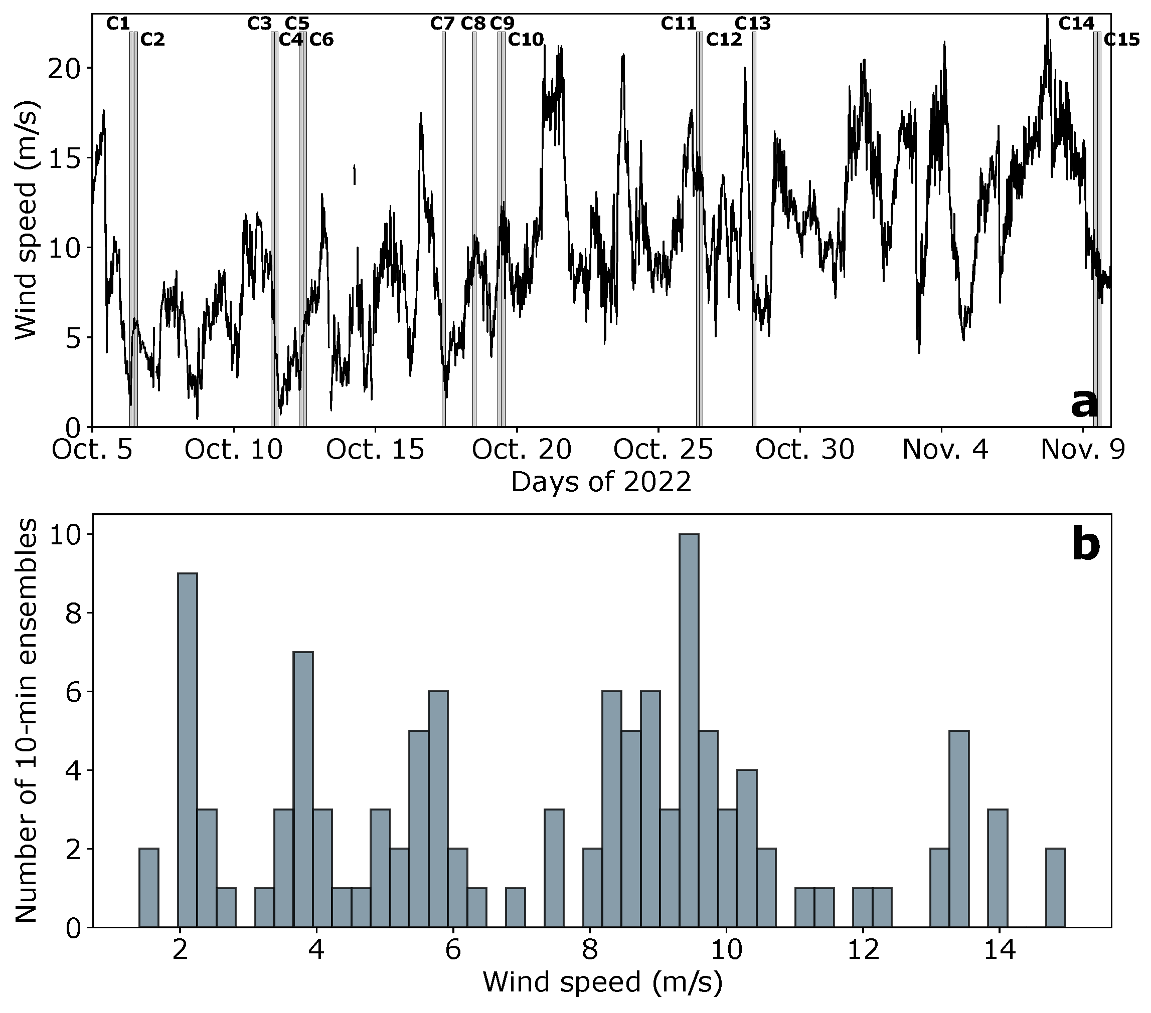
The fixed lidar operated continuously for a duration of 57 days, spanning from 14 September to 9 November 2022. On the other hand, the mobile lidar was activated and deactivated on specific dates within the same period to avoid data collection during rainy days (
Table 2,
Figure 2a). A total of 15 measurement cycles were recorded between 6 October 2022 and 9 November 2022. Each cycle consisted of nine 10 min regular sequences involving rotations around the
y-axis at various amplitudes and periods, as well as movements that coupled rotations around different axes, namely (i)
x and
y, (ii)
y and
z, and (iii)
x,
y, and
z (
Table 3). The dataset was enriched with a 2 h data acquisition period during which both instruments remained stationary, allowing for a comparison of their measurements in the absence of movement.
The signals from both lidars were divided into 10 min ensembles, each containing 600 data points. The two lidars recorded data at 10 different measurement heights, evenly distributed between 40 m and 220 m. Note that achieving synchronous collection of LOS velocity from both lidars was not possible due to the inability to configure the starting point of data collection for the lidar beams. Consequently, recordings of sequences measured by the fixed and mobile lidars displayed a temporal offset between them, ranging from a minimum of 0.05 s to a maximum of 0.71 s.
Over the course of 45 h of data collection by both lidars, data availability consistently maintained at 100% at each measurement altitude. It is worth noting that, in this work, the prototype configurations of the lidars employed a data availability threshold of −21.5 dB, as opposed to the −23 dB threshold used in the commercial configuration. This specific threshold adjustment was made to address the anticipated reduction in data availability due to the need for shorter accumulation times in order to achieve the higher sampling rate. With a threshold set at −23 dB, the data availability averaged around 99.4% with a decrease over increasing altitude.
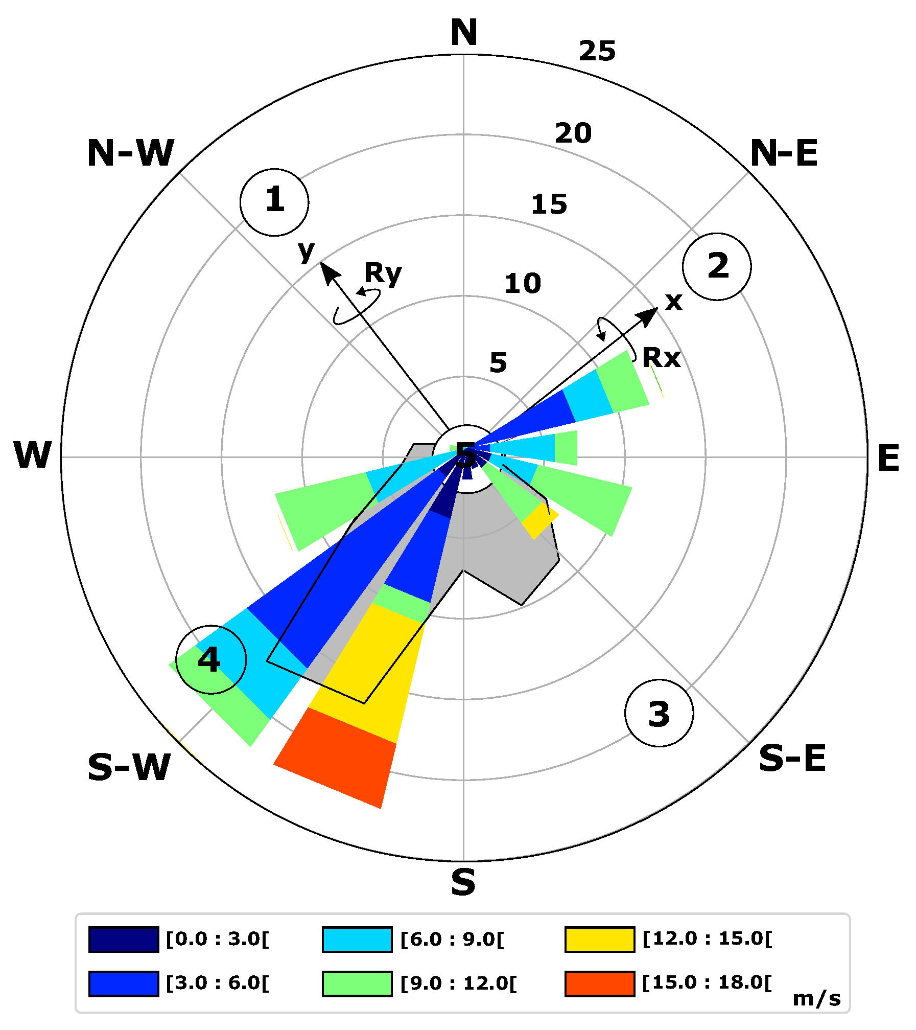
At the test site, wind characteristics captured by the fixed lidar over the 57-day deployment period indicated wind speeds ranging between 0.5 m/s and 23.3 m/s, with a mean of 10 m/s at 140 m above the ground. The prevailing wind directions were predominantly from two main sectors: the South-West and the South-East (indicated by gray shading in
Figure 3). These sectors align with the average wind directions recorded during the 15 measurement cycles of the mobile lidar (depicted by boxes in
Figure 3). Moreover, the 15 cycles encompassed various wind speed ranges, with speeds ranging from 1.2 m/s to 17 m/s and a mean of 7.5 m/s at 140 m above the ground (
Table 2,
Figure 2b).
2.3. Motion Specifications
The hexapod was configured to simulate the possible motions of a moored floater. France Energies Marines developed a large buoy, known as MONABIOP, deployed at the Mistral test site in the Mediterranean Sea. While it is important to note that commercial FLS often use single-point moorings, MONABIOP employs a distinct mooring system with three semi-taut lines to restrict its motion. This design is primarily intended for testing and validating a mooring system that utilizes nylon ropes. It is worth acknowledging that while MONABIOP’s motion dynamics may not precisely replicate all aspects of commercial FLS systems, it provides valuable insights into the behavior of buoy-like structures in dynamic marine environments. The buoy’s dynamics, mainly governed by the tilt having a natural period of 4 s, was used as a reference for defining different motion scenarios for the hexapod.
The amplitude of tilt motion experienced by a FLS is dependent on the prevailing sea state. In very calm seas, minimal dynamic tilt motion is anticipated. However, in the presence of strong waves, the floating platform experiences significant excitation, resulting in larger tilt motions. Amplitudes of 5 deg. and 15 deg. were selected to represent medium and high tilt motions, respectively. These amplitudes represent those of a FLS deployed in a real sea environment [
9].
The tilt motion period of a FLS is type specific and determined by its mass and hydrodynamic properties. Three periods were chosen: the natural period of the MONABIOP buoy (4 s), twice its natural period (8 s), and an intermediate value (6 s). Consequently, nine cases were chosen to cover a wide range of motion scenarios while minimizing the number of cases needed (
Table 3). Initially, rotations around a single axis, Ry, were applied, followed by the gradual addition of rotations around one and two other axes, Rx and Rz. The phase of Ry was fixed at 0, Rx was set to
, and Rz was set to
/2.
2.4. Assessing Motion-Induced Effects: Evaluation Metrics
Turbulent velocity fluctuations were assessed by computing the standard deviation, denoted as
, from the mean-detrended signal derived from 10 min ensembles of the LOS velocities as well as the along-wind and cross-wind velocities. This process involved the removal of the mean value (i.e., the constant component), effectively centering the data around zero through subtraction of the mean from the original signal. For the LOS velocity, the focus was on beam 1 and beam 2, which are positioned at 90° to each other (
Figure 3). Motion-induced effects observed in beam 3 closely mirror those seen in beam 1, with both beams positioned opposite each other. Likewise, the motion-induced effects observed in beam 4 closely resemble those in beam 2, with both beams facing each other.
The impact of motion-induced effects on turbulent velocity fluctuations measured by FLS was assessed by calculating the root-mean-square error (RMSE) of the turbulent velocity fluctuations obtained from the fixed and mobile lidars noted respectively as
and
for each 10 min ensembles,
i, such as
The initial measurements from the first 6 sequences, spanning 15 cycles, were specifically chosen to examine the impact of rotation amplitude and period around the
y-axis (refer to
Table 3) on the RMSE of velocity fluctuations. Additionally, the impact of various factors such as wind speed, wind direction, and wind shear was investigated. Following this analysis, the effects of coupling multiple rotations were further evaluated using sequences 7, 8, and 9 of the 15 cycles.
3. Results
3.1. Statistical Significance
To ensure the relevance of the presented results, statistical significance was assessed through the determination of a significance level, commonly set at 0.05 or 5% (e.g., [
16]). Initially, a null hypothesis was formulated, positing that variations in RMSE for each motion scenario occur randomly and are unrelated to the main factors under investigation: wind speed, wind direction, motion amplitude and period, measurement height, and wind shear.
For each scenario, recorded 15 times, RMSE values were computed at 10 different altitudes, resulting in 150 RMSE measurements associated with the factors examined in our study. Subsequently, for each pair of variables, such as RMSE and wind speed (each with 150 values) or RMSE and wind direction, a corresponding p-value was computed. The p-value represents the probability that the observed difference could have arisen solely by random chance.
In our analysis, the calculated p-values ranged from 0.0063 to 0.0097, notably lower than the threshold of 0.05. This indicates that the observed results are highly unlikely to be explained solely by chance, warranting the rejection of the null hypothesis. Consequently, our experiment and its associated findings are statistically significant.
3.2. Preliminary Observations
The analysis begins by examining the turbulent fluctuations measured by both lidars, without motions. Throughout the entire measurement campaign, these lidars operated independently and were positioned 10 m apart, leading to the measurement of distinct air volumes. Such disparities in measurement can potentially introduce gaps in the estimation of the standard deviation, , of LOS velocities.
The average
, associated with beam 1, as measured by the fixed lidar, was determined to be 0.719 m/s. In contrast, the average
obtained from the mobile lidar measurements was slightly higher, specifically by 0.8%, resulting in a value of 0.713 m/s. A graphical comparison of
derived from both lidars can be observed in
Figure 4a. To further assess the agreement between the measurements made by these instruments, a linear regression analysis was conducted on the distribution, yielding an R
2 value of 0.99. This high R
2 value signifies a strong concordance between the measurements obtained from both lidars.
The impact of motion was subsequently evaluated, comparing LOS velocity time series obtained from fixed and mobile lidars.
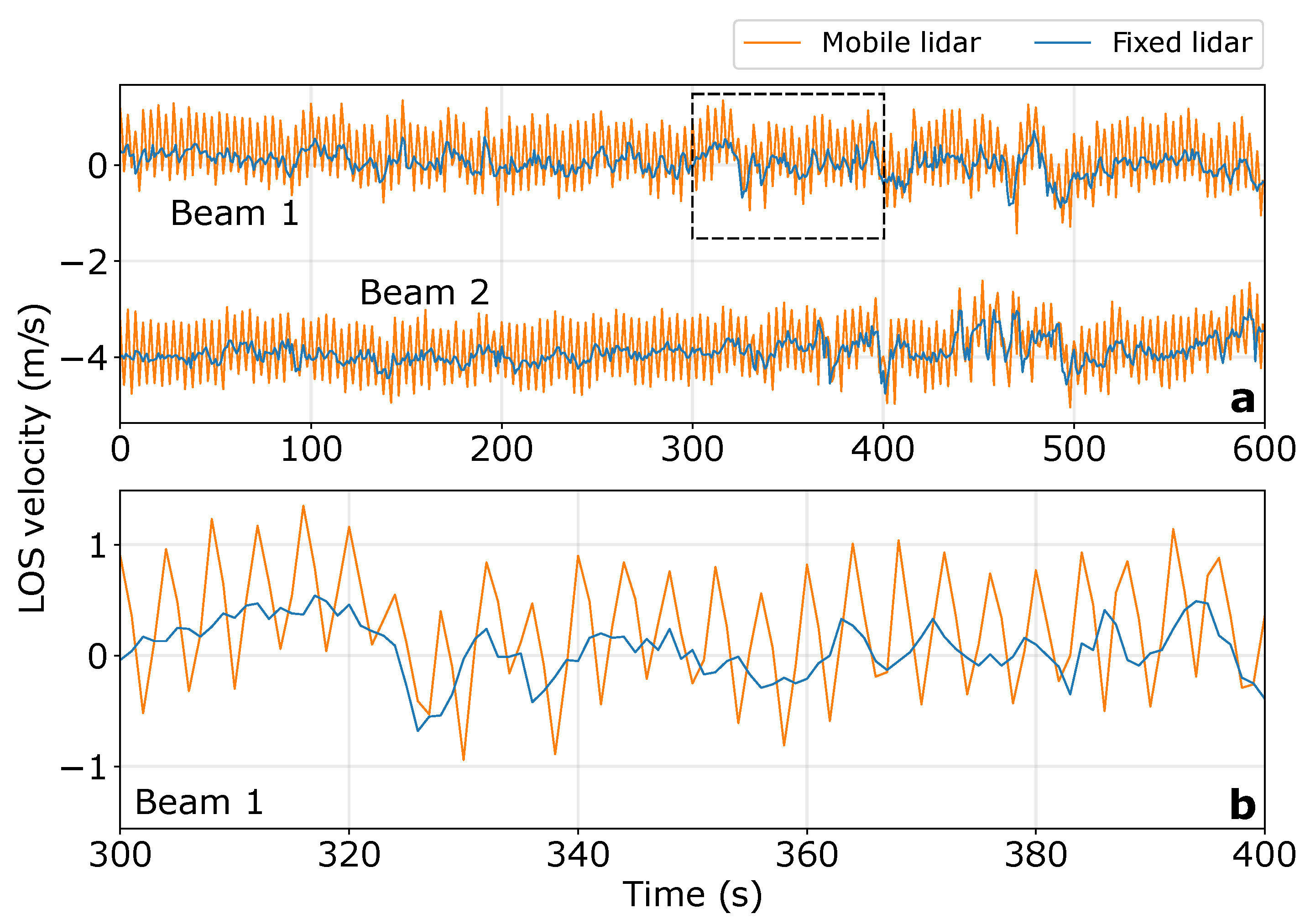
Figure 5 illustrates this analysis for sequence 1 of cycle 13 at a measurement altitude of 140 m. The comparison of beam 1 and beam 2 reveals that the mobile lidar captures the shape of the velocity patterns observed in the fixed lidar measurements (
Figure 5b). Moreover, the oscillations observed in the mobile lidar measurements clearly indicate the impact of regular motion on the device. In this particular sequence, these oscillations result in a standard deviation (∼0.50 m/s) of the LOS velocities that is twice as high as the standard deviation computed from the fixed lidar measurements.
Figure 4b reveals a predominantly consistent trend of overestimation in
measurements by the mobile lidar compared to those derived from the fixed lidar, with few exceptions. Considering all measurement heights and sequences collectively, the mean
measured by the fixed lidar was found to be 0.45 m/s, while the mean
from the mobile lidar measurements was approximately 70% higher.
3.3. Impact of Motion Amplitude and Wind Speed
In
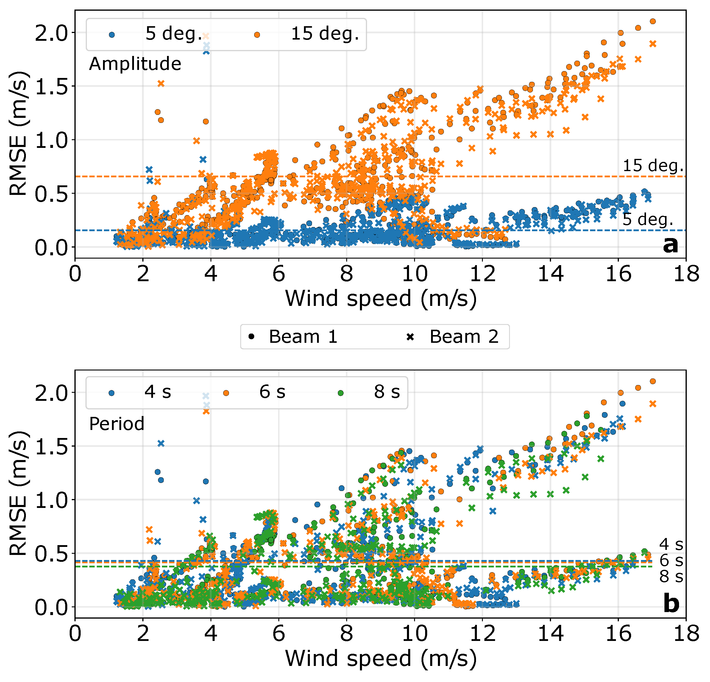
Figure 6a, it is evident that higher amplitudes correspond to increased RMSE values for a given period. At a lower amplitude (5 deg.), the mean RMSE associated with beam 1 is 0.15 m/s. However, with an amplitude three times higher, the mean RMSE increases to more than four times higher (0.65 m/s). At the lowest amplitude, the RMSE associated with beam 1 reaches 0.5 m/s at higher wind speeds, while for the highest amplitude, it reaches 2 m/s. Although the RMSE values associated with beam 1 and beam 2 are similar at the lowest amplitude, the gap between the RMSE values derived from both beams slightly widens at higher wind speeds. Conversely, at the highest amplitude, the RMSE associated with beam 1 is consistently higher than that associated with beam 2.
Furthermore, wind speed has a clear impact on RMSE. Our results demonstrate that RMSE increases with higher wind speeds, particularly noticeable for higher amplitudes of motion. However, this increase is not linear. Within certain wind speed ranges, such as [2; 4] m/s or [4; 6] m/s, there are abrupt increases in RMSE, particularly pronounced for the highest amplitudes. This finding suggests that amplitude and wind speed are not the sole determinants of RMSE and implies that wind direction may also play a significant role.
3.4. Impact of Wind Direction
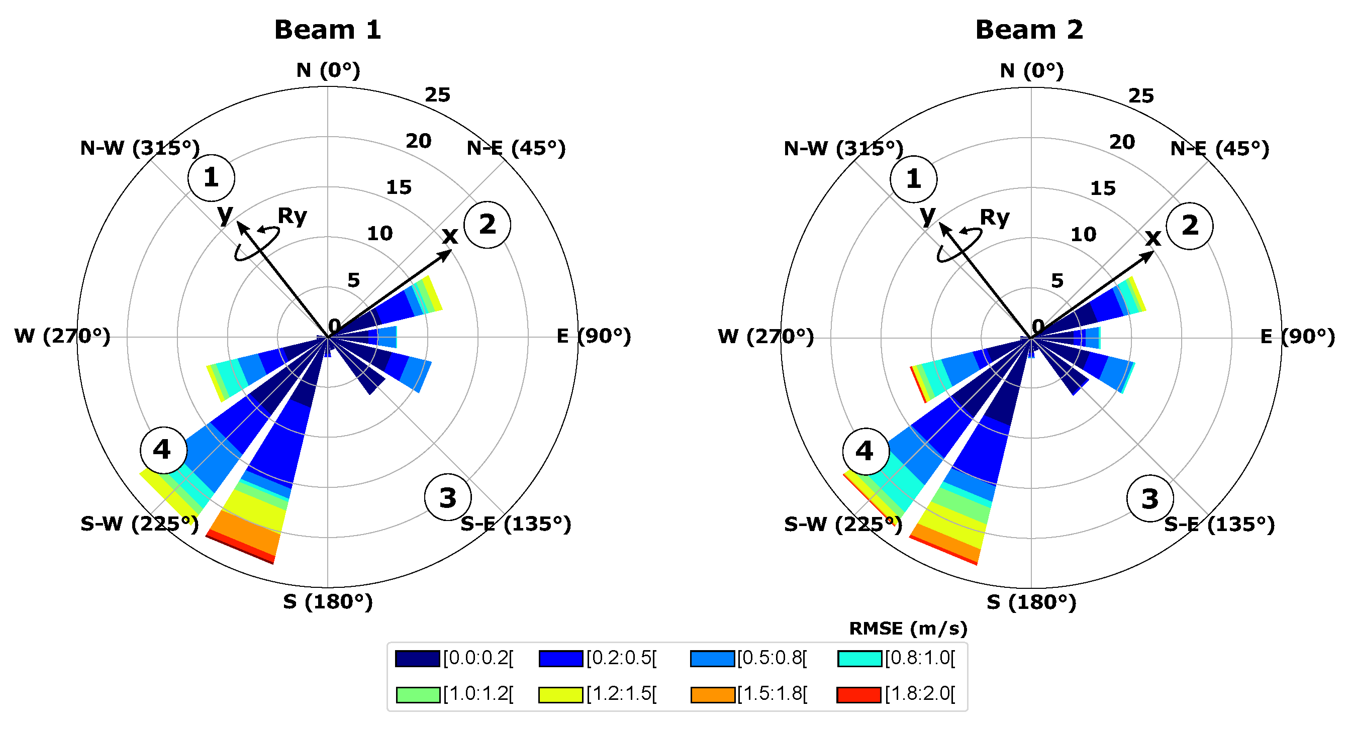
The examination of RMSE wind roses for beam 1 and beam 2 (
Figure 7) reveals a consistent pattern: the highest RMSE values coincide with the mobile lidar’s tilt direction aligned with the wind direction. Comparing this polar distribution of RMSE with the wind speed distribution (
Figure 3) for beam 1 and beam 2, a notable finding emerges: despite lower wind speeds (averaging 6 m/s) during the mobile lidar’s tilt alignment with the wind compared to its perpendicular orientation (averaging 7.6 m/s), the mean RMSE surpasses values more than 10 times higher when the wind aligns with the mobile lidar’s tilt direction. These results strongly emphasize the substantial impact of wind direction on turbulence measurement accuracy. They highlight the critical necessity of rigorously accounting for wind direction effects in turbulence data analysis derived from FLS measurements.
3.5. Impact of the Motion Period
The influence of the motion period on RMSE values is illustrated in
Figure 6b. As observed, a decreasing trend is evident: as the period decreases, the RMSE tends to increase. However, it is notable that the mean RMSE values calculated for the three periods scenario are relatively similar. For instance, the mean RMSE associated with a 4 s period was determined to be 0.43 m/s, representing a 14% increase compared to a period twice as long. This finding underscores how the impact of the motion period is mitigated when contrasted with the factors examined in previous sections.
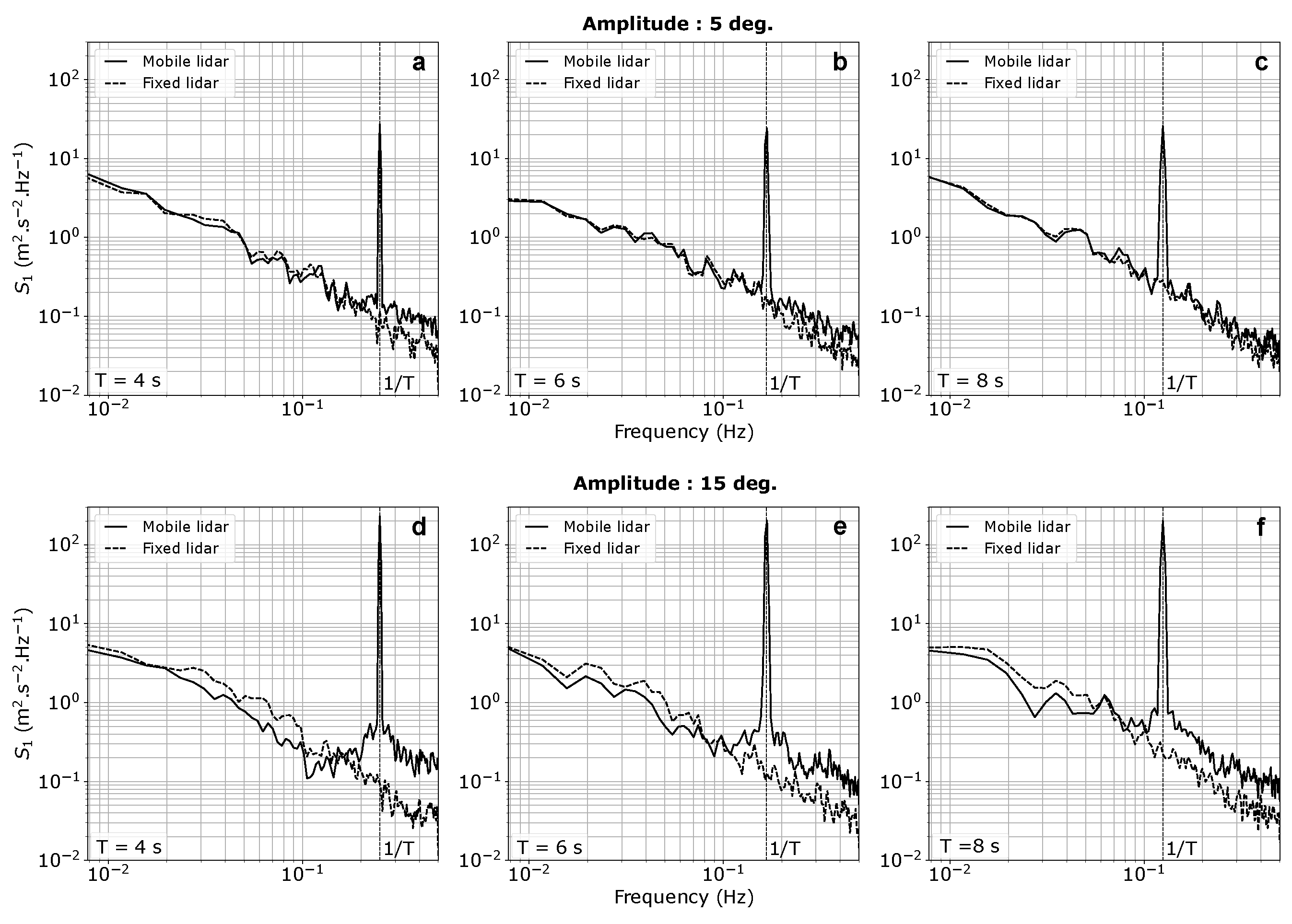
Moreover,
Figure 8 shows that the motion period significantly influences the LOS velocity spectra. The mean spectrum is presented, averaged over 15 cycles and measured at 140 m above the ground by beam 1 of both the mobile and fixed lidars. The spectra obtained from the mobile lidar clearly exhibit a spike in energy corresponding to the rotation frequency. The height of this spike remains consistent for each motion period and is lower for the lowest amplitude. For both amplitudes, the spectral energy measured by the mobile lidar surpasses that of the fixed lidar for the higher frequencies. Moreover, this difference in spectral energy becomes more pronounced for the lowest motion period. Conversely, at lower frequencies, the spectral energy associated with a 15 deg. amplitude, derived from measurements of the fixed lidar, consistently surpasses that of the mobile lidar. In the case of a 5 deg amplitude, the spectral energy derived from measurements of both fixed and mobile lidars shows overlap.
3.6. Impact of Measurement Height
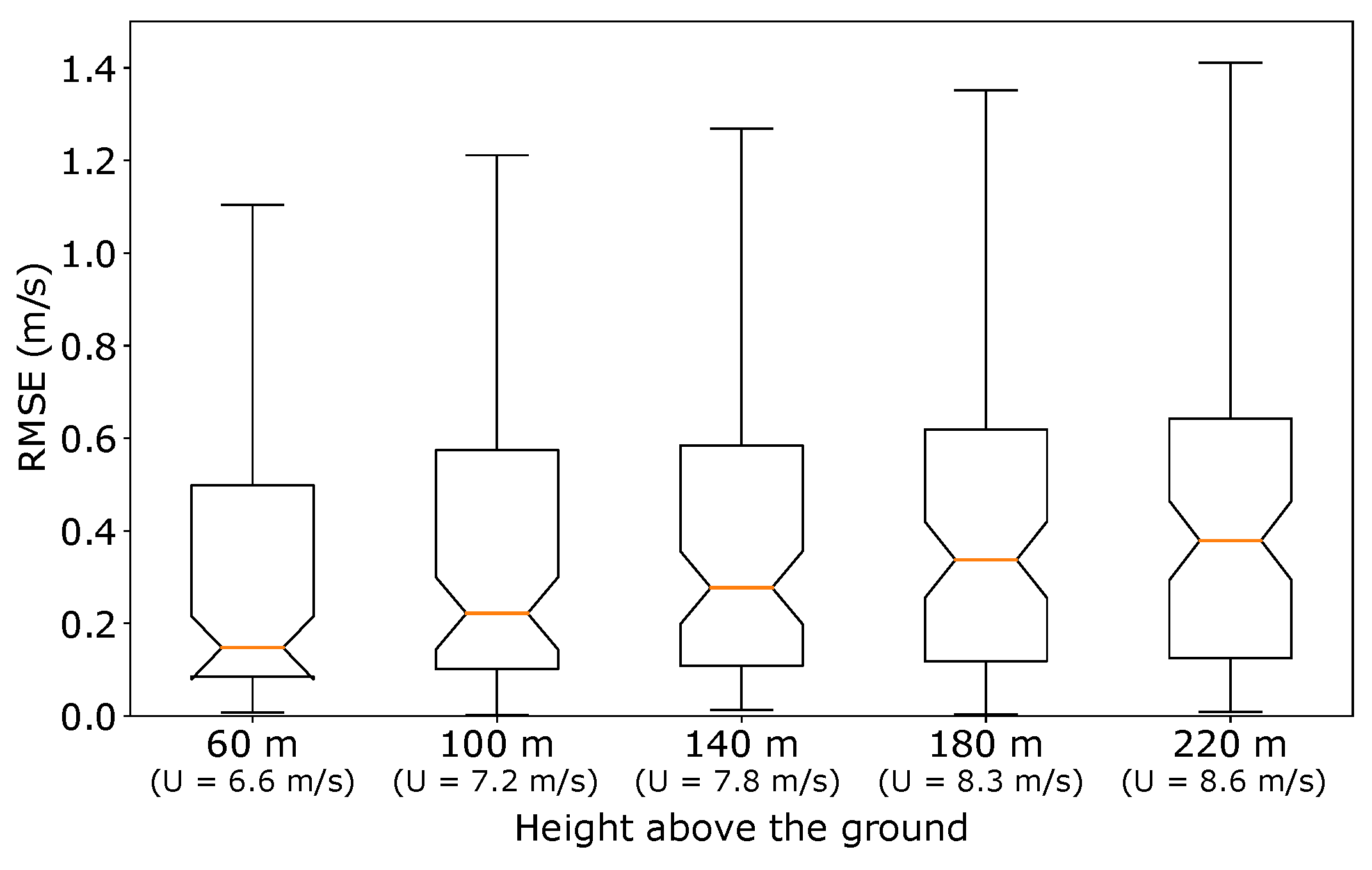
Figure 9 illustrates a significant trend: the RMSE shows an upward trend as the measurement height increases. Notably, at an altitude of 220 m, the median RMSE exceeds the median value of 0.15 m/s computed at 60 m by more than 2.5 times. This observation aligns with the expected outcome, as previous findings in this study have demonstrated that higher wind speeds lead to higher RMSE in velocity fluctuations.
Although the mean wind speed at 220 m was found to be 30% higher than the wind speed computed at 60 m, it is essential to acknowledge that wind speed alone may not be the sole factor influencing the RMSE of LOS velocity fluctuations when considering the impact of measurement height. The rotational displacements of the mobile lidar cause the beam direction to tilt compared to the fixed lidar, resulting in the shifting positions of focus points both vertically and horizontally. Consequently, the mobile lidar does not scan the same volume of air as the fixed lidar, potentially missing out on sampling the same eddies. This effect becomes more pronounced with increasing measurement height. Moreover, the increase in the RMSE at higher measurement heights might also be due to the vertical gradient of the horizontal mean wind speed which is known to impact the wind vector measured by a FLS [
9].
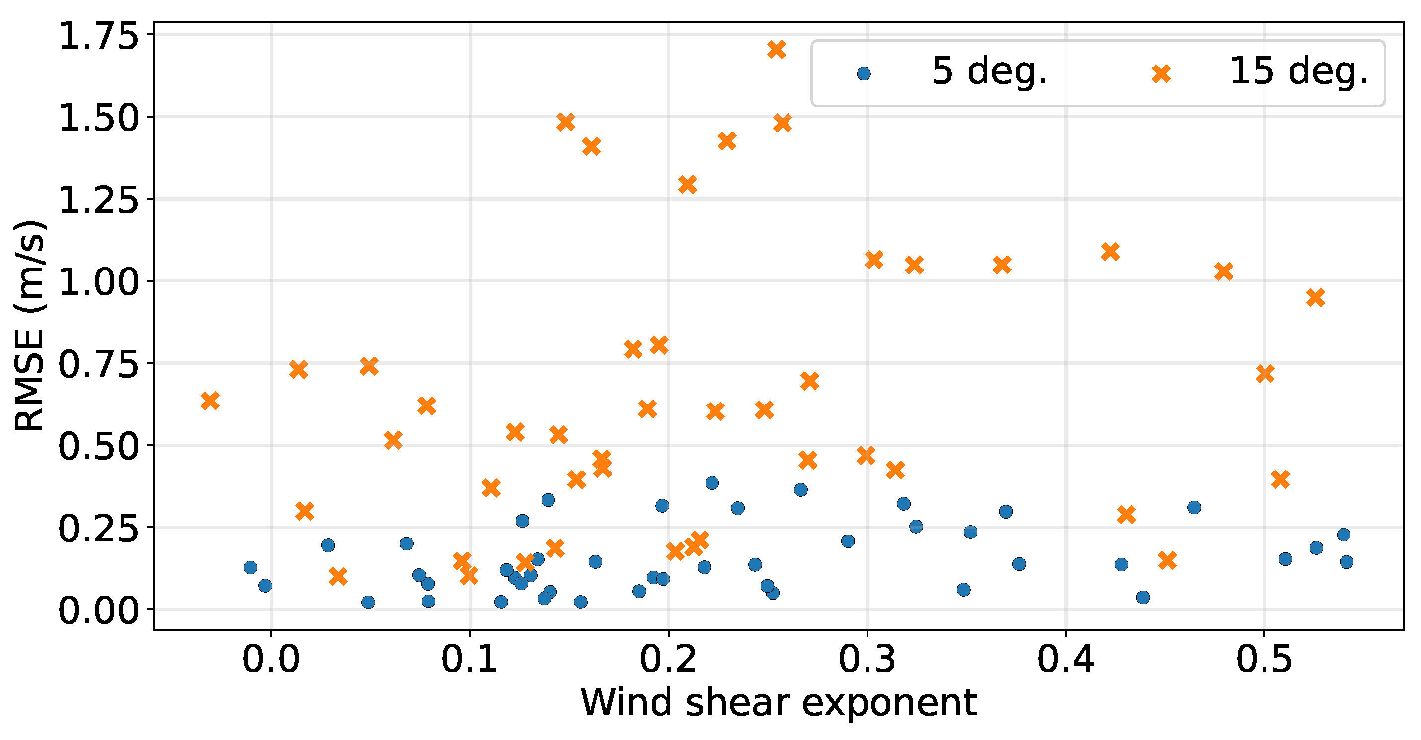
3.7. Impact of Wind Shear
In the presence of a sheared wind speed profile with usually higher wind speeds at higher altitudes, the changes in measurement heights have an influence on the mean wind speed. In this study, we assessed the impact of wind shear on the RMSE of the LOS velocity fluctuations by examining the first 6 sequences out of the total 15 cycles.
To determine the wind shear exponent,
, we employed individual 10 min average wind speed vertical profiles derived from measurements obtained by the fixed lidar. These profiles were then fitted using the power law profile recommended by the IEC 61400-3-1international standard [
17]. The fittings yielded a mean relative error of less than 1%.
Figure 10 shows that the height-averaged RMSE of the LOS velocity fluctuations is not governed by the wind shear exponent which varies from −0.05 to 0.55. The RMSE associated with one single rotation of 5 deg. amplitude shows a slight variation around the mean of 0.15 m/s for the entire range of the computed wind shear exponents. Similar results are found for the RMSE associated with one single rotation of 15 deg. amplitude with a more scattered distribution around the mean of 0.65 m/s and extremes values higher than 1.25 m/s. Those extreme values are found for a wind shear exponent of 0.2 on average and are associated with wind speed ranging between 13 and 14.5 m/s and wind direction aligned with the tilt direction of the mobile lidar.
Therefore, while the findings indicate that the wind shear exponent may not exert a dominant influence on RMSE, they suggest a complex relationship between wind shear and turbulence measurements, acknowledging that other contributing factors, as shown previously, are likely influential in shaping the accuracy of turbulence data obtained with a FLS.
3.8. Impact of the Coupling of Motions around Several Axis of Rotation
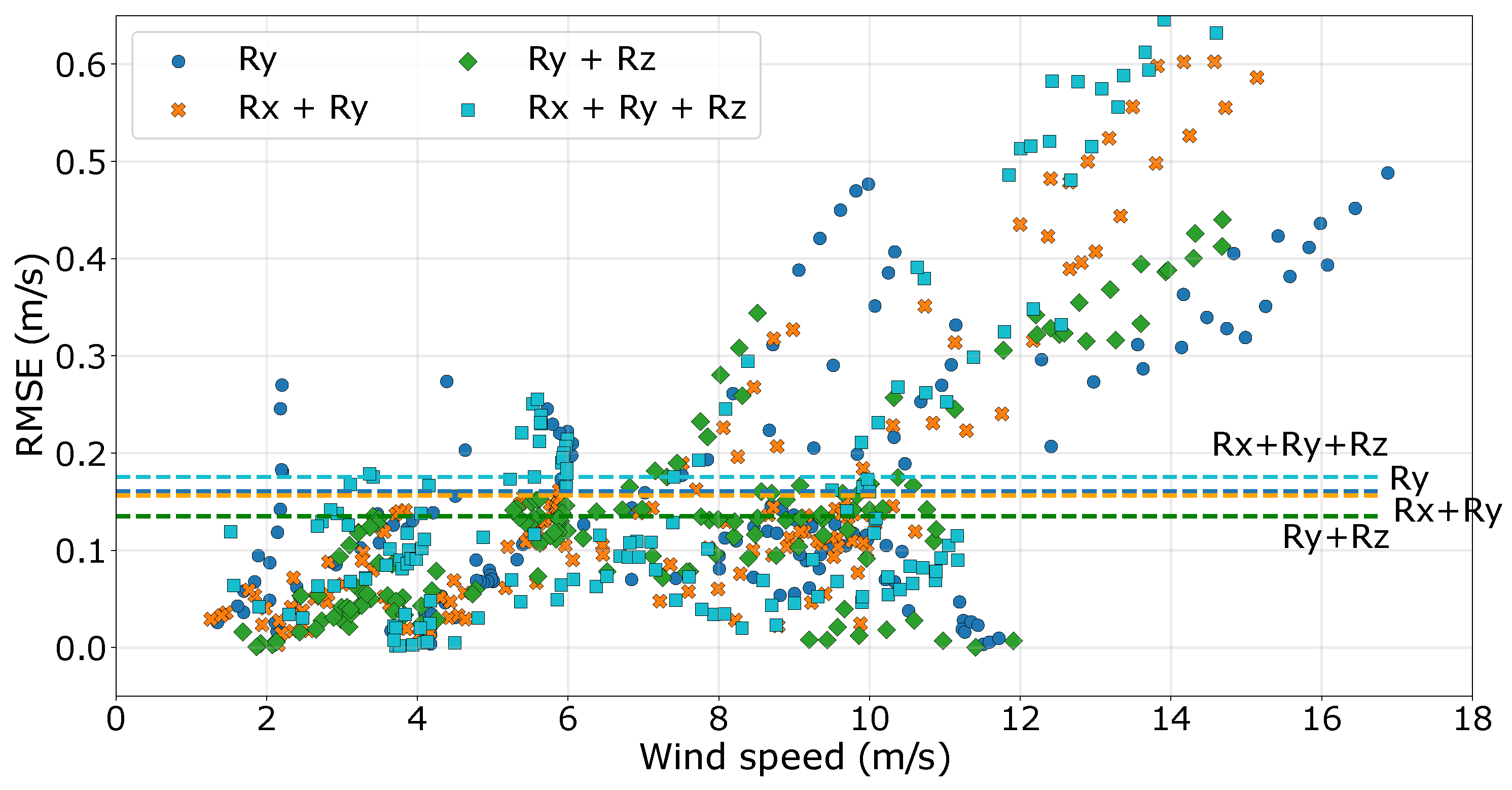
The coupling of the three rotations Rx, Ry, and Rz resulted in the highest RMSE, as shown in
Figure 11. The coupling of two rotations, i.e., Rx/Ry (phase shift of
between both motions) and Ry/Rz (phase shift of
/2 between both motions), did not lead to significant differences in RMSE values when compared to the single rotation Ry.
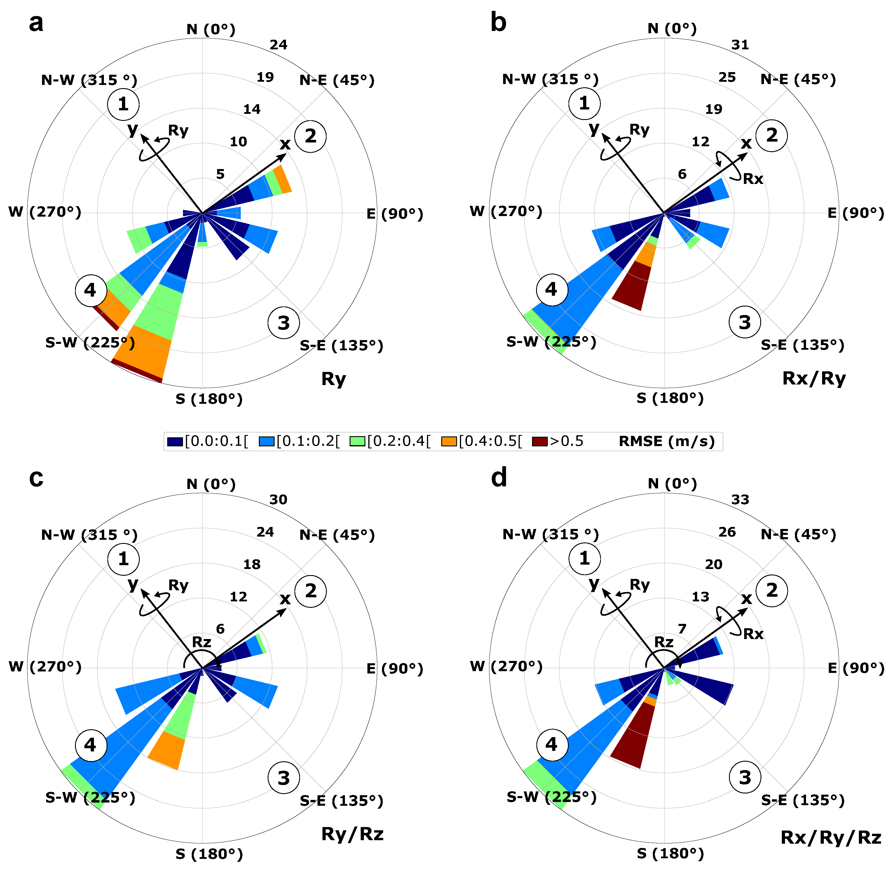
The coupled rotation Ry/Rz has been tested to evaluate the impact of yaw, i.e., rotation around the
z-axis, on RMSE values. The low restoring forces associated with yaw motion, resulting in correspondingly low motion frequencies, may contribute to fluctuations in the time series of LOS velocity that are not primarily due to wind-induced turbulence but rather motion-induced turbulence. However,
Figure 12c shows that similarly to results associated with the single rotation Ry (
Figure 12a), the coupled rotation Ry/Rz produced high RMSE when the wind was perpendicular to the
y-axis but yielded low RMSE when the wind aligned with this axis. These findings imply that yaw motion likely has a negligible impact on RMSE values. However, this hypothesis would require confirmation through isolated motion along the
z-axis, a scenario not explored in our study.
Moreover,
Figure 12b,d shows that rotations Rx/Ry and Rx/Ry/Rz did not exhibit a consistent pattern, possibly due to variations in the phase of these coupled motions. When the wind aligns with either the
x-axis or the
y-axis, it can generate both high and low RMSE values. These findings suggest the potential significance of considering the phase of rotational motions in the context of turbulence analysis and LOS velocity, as it may have an impact on turbulence measured by a FLS. However, it should be noted that these observations do not conclusively prove the influence of phase shift. One potential explanation for the limited impact of phase on RMSE values could be attributed to the lack of synchronization between motion and scanning strategies, resulting in the appearance of unsynchronized motion phases. Further experimentation with varying phases is necessary to gain a comprehensive understanding of the relationship between motion phases and RMSE values.
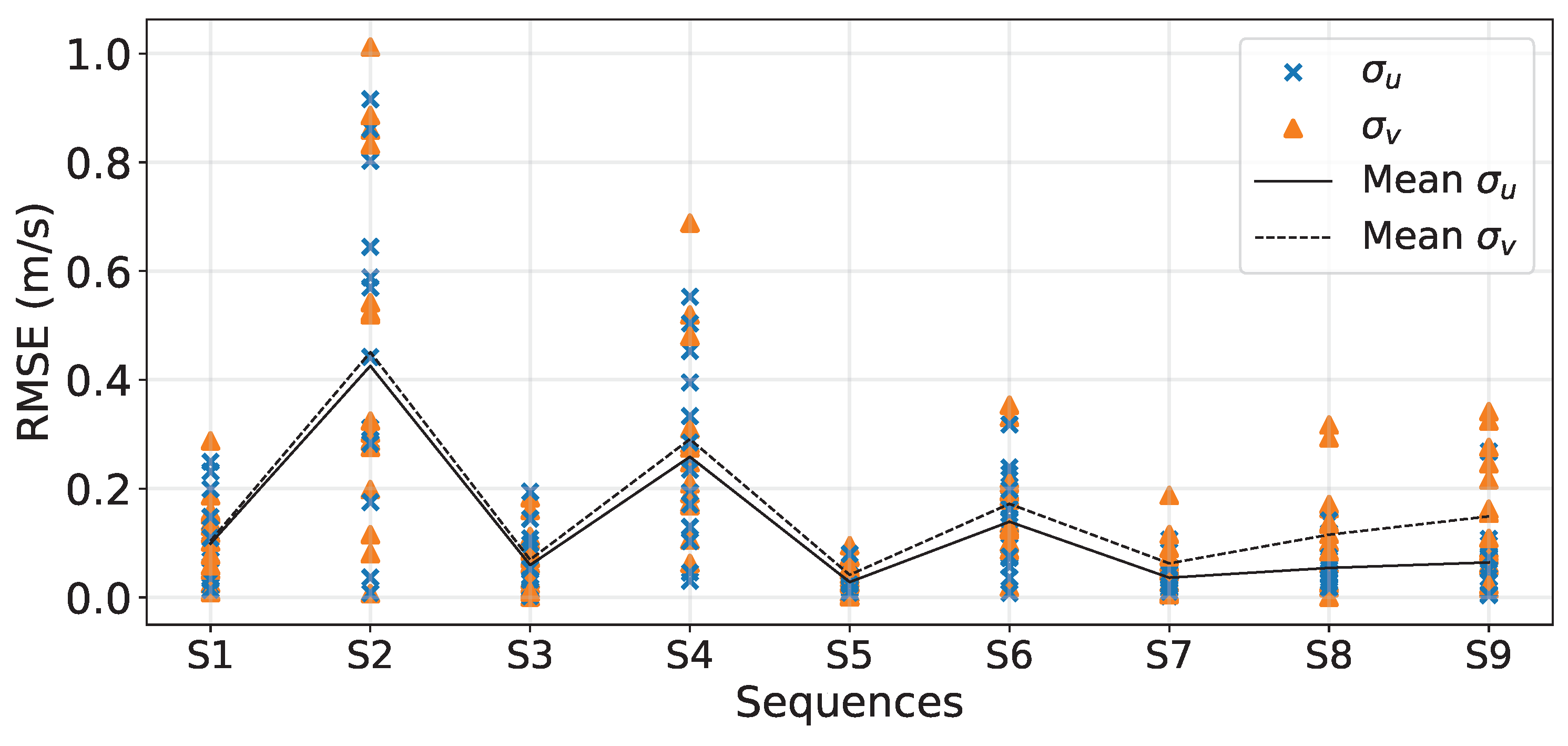
3.9. Global Impact on Along-Wind and Cross-Wind Velocity Fluctuations
The preceding sections have aimed to pinpoint the primary source of error in turbulent velocity fluctuations as measured by a lidar profiler, particularly focusing on LOS velocity fluctuations. However, LOS measurements are not extensively utilized within the wind energy community. Instead, turbulence characterization heavily relies on the standard deviation of both the along-wind and cross-wind components, denoted as
and
, respectively. These metrics are pivotal in calculating TI along both directional axes.
and
were calculated from the reconstructed velocity components (Equations (
1) and (
2)), and then they were rotated along and across the direction of the wind.
In
Figure 13, observations reveal that in scenarios with a singular axis of rotation (
Table 3), the sequence displaying the shortest period and highest amplitude (S1) exhibits the highest RMSE for both
and
. Conversely, the lowest RMSE is associated with the longest period and lowest amplitude (S5). Notably, the RMSE for
consistently exceeds that of
, and this disparity amplifies with longer periods and the incorporation of additional axes of rotation.
While the introduction of multiple axes of rotation (S7-9) minimally affects , maintaining a comparable RMSE to that of a single rotation with low amplitude, the RMSE of significantly escalates with added rotation axes. For instances with similar amplitudes and periods, the RMSE of in motion involving three axes of rotation (S9) is doubled that of motion around a single axis (S3).
4. Discussion
The motivation for the results presented in this paper arose from a noticeable absence of statistically relevant experimental testing in the literature, specifically addressing the evaluation of motion-induced effects on turbulent velocity fluctuations measured by a FLS. Also, most of the studies were performed numerically and focused on the mean wind statistics and not on turbulence.
While [
13] proposed a similar experiment to ours, they recorded different motions along only one axis of rotation, and these were captured only once during a 3 h period. Consequently, the statistical significance of their results is called into question due to the low variability of wind speed and directions recorded during each scenario. In contrast, our study addresses this limitation by conducting multiple recordings of diverse scenarios over several weeks. This approach allows for gathering sufficient wind variability, thereby facilitating the identification of the primary factors influencing the error in turbulence measurement collected by a FLS. The results of our experiments demonstrate that the alignment between wind direction and direction of tilt of the mobile lidar plays a critical role in determining the accuracy of turbulence measurement. When the tilt of the mobile lidar leans in the wind direction, resulting in pitch motion, it introduces high motion-induced turbulence. This pitch-induced turbulence leads to higher RMSE values in velocity fluctuations. Conversely, when the tilt of the lidar leans perpendicular to the wind direction, resulting in roll motion, the lidar’s motion harmonizes with the wind flow, reducing motion-induced turbulence and consequently leading to lower RMSE values. The impact of wind direction on turbulence measurement with regards to the tilt of the lidar is in agreement with previous simulation studies performed by [
9] focusing on mean wind speed. Thus, our experimental results demonstrated that the main factor affecting the mean wind statistics measured by FLS are like those affecting the turbulence statistics.
Although no definitive evidence of yaw’s impact emerged from our study, it is important to note that yaw was involved in rotations around multiple axes. However, specific scenarios solely focusing on yaw rotation were not scheduled. Despite previous findings indicating that yaw has a significantly lower impact on mean wind statistics compared to pitch and roll [
9], it is expected that the lower motion frequencies associated with yaw, coupled with its relatively low restoring forces, might still contribute to elevated RMSE values.
Furthermore, our study sheds light on the influence of motion across various axes of rotation. This specific point also fills a gap in the literature. Results showed that motion around all three axes yield to higher RMSE values. However, it is worth noting that this study’s experimental design places some limitations on drawing firm conclusions regarding the effects of coupled rotations on turbulent fluctuations measured by FLS. Further inquiry is warranted, with a focus on exploring various phase shifts. Moreover, this study does not delve into translational motion, which is a common occurrence alongside rotations in real FLS scenarios. These translational movements affect the measurement of mean wind statistics as demonstrated in [
9] and are expected to affect turbulence measurement, contingent upon factors like oscillation frequency and peak velocity relative to wind speed. Thus, comprehensive research is required to provide a more thorough understanding of these effects.
This study provides valuable insights into the relationship between wind speed, measurement height, and velocity fluctuations. The findings show that as wind speed increases, the differences in velocity fluctuations between the fixed and mobile lidars also increase. This observation is particularly significant because it highlights the sensitivity of turbulence measurement to wind speed variations over short distances. Spatial variability in turbulence, which can differ significantly in close proximity, is amplified by the continuous movement of the mobile lidar. As a result, when wind speed is higher, spatial turbulence variability tends to increase, leading to larger discrepancies in measured turbulence values.
Furthermore, the increase in RMSE with measurement height corresponds to a well-known trend in atmospheric science, where mean wind velocities tend to increase with altitude due to decreasing surface roughness influence. The RMSE values, being governed by wind speed magnitude, follow a similar trend. However, it is essential to acknowledge that other factors, such as wind shear, may also contribute to the observed RMSE variations. While wind shear is expected to play a role, its exact impact remains complex and not entirely evident in this study. This complexity may be attributed to lidar probe volume size, geometry, and data averaging over time, which can mitigate sensitivity to rapid wind shear changes.
This study highlights that turbulence measurements obtained from FLS are more sensitive to changes in orientation (amplitude of motion) than to motion periods. This finding underscores the significance of changes in measurement geometry due to platform orientation. The analysis revealed a strong correlation between high RMSE and high amplitude. Additionally, it was observed that amplitude significantly influences the measurement of spectral energy, particularly in the low-frequency domain, associated with high turbulence length scales. To the best of our knowledge, this finding was not evidenced in the existing literature since the impact of motion on velocity spectra was not addressed in previous studies. When the lidar system tilts, it effectively acquires data from diverse air masses and turbulence conditions, resulting in fluctuations in turbulence measurement. These variations can be significant, especially when the amplitude is high, and it is crucial to take these factors into account during data interpretation.
Conversely, the impact of the motion period on RMSE values was found to be limited compared to amplitude. Turbulence is characterized by rapid and stochastic fluctuations in wind speed and direction, and periodic motion alone does not inherently change turbulence statistical properties. However, this study observed energy spikes in LOS velocity spectra at specific frequencies corresponding to motion periods. These spikes indicated increased spectral energy associated with mobile lidar measurements in the expected inertial sub-range. Following these spikes, within the high-frequency range, the spectral energy linked to the mobile lidar measurements consistently surpasses that of the fixed lidar measurements. This difference becomes more pronounced as motion periods decrease. The observed differences in spectral energy between the mobile and fixed lidar suggest that the spatial and temporal averaging characteristics of the two systems play a role in turbulence measurement. Fixed lidar systems, with longer measurement durations at specific locations and more extensive temporal averaging, tend to smooth out high-frequency turbulence fluctuations, resulting in lower spectral energy in the high-frequency domain compared to the mobile lidar. This demonstrates the importance of considering both spatial and temporal averaging effects when comparing turbulence measurements from different platforms.
5. Conclusions
The present study experimentally corroborates previous numerical findings documented in the literature. The high variability in wind speed and direction recorded during our experiment has enabled us to draw robust conclusions regarding the primary factors impacting measurements with a FLS. It has been demonstrated that the main factors influencing turbulence measurement with a FLS align closely with those affecting mean wind statistics.
Investigating single-axis rotations revealed that the predominant influencing factor on turbulence measurement with a FLS is the alignment between the tilt direction of the mobile lidar and the wind direction. Pitch motion resulted in the highest RMSE values, whereas roll motions yielded the lowest RMSE values. Moreover, the introduction of motion around additional axes of rotation was found to increase RMSE.
Nevertheless, there exists a necessity for real-life comparisons to effectively demonstrate the practical implications of our experimental findings. Moving forward, integrating real wind field data or employing numerical simulations representing actual scenarios will enhance the relevance and applicability of our conclusions. This approach will facilitate direct comparisons between our experimental results and real-world atmospheric dynamics, providing a clearer understanding of the implications of motion on FLS measurements.
Furthermore, future research endeavors should prioritize the development and exploration of motion-compensation algorithms using the dataset presented in this study. Such algorithms hold promise for mitigating motion-induced turbulence and improving the quality of turbulence measurements obtained from lidar profilers. By integrating numerical modeling and investigating motion-compensation techniques, we can advance our understanding of atmospheric dynamics and contribute to the development of innovative technologies for renewable energy and environmental monitoring.
In summary, our study underscores the importance of addressing motion effects in FLS measurements and highlights avenues for future research. By incorporating real-life comparisons and exploring motion-compensation strategies, we can further enhance the reliability and applicability of turbulence measurements obtained from FLS, ultimately advancing our understanding of atmospheric processes and supporting the development of sustainable energy solutions.
Author Contributions
M.T. identified the problematic, analyzed the results, drafted this paper, and plotted the figures. N.T. processed the raw data under the supervision of M.T. G.D., M.L.B., C.M. and M.T. who designed the experiment. M.L.B., C.M., C.B. and F.G. reviewed this paper. All authors have read and agreed to the published version of the manuscript.
Funding
This work was made possible through the support of France Energies Marines and the French government, managed by the Agence Nationale de la Recherche under the Investissements d’Avenir program, with the reference ANR-10-IEED-0006-34. This work was carried out in the framework of the POWSEIDOM project.
Data Availability Statement
The data is owned by a public-private consortium with proprietary rights and confidentiality obligations, precluding its sharing alongside this paper.
Acknowledgments
We would like to acknowledge the team at Vaisala, including Mathias Régnier, Loïc Mahe, Frédéric Delbos, and Hugues Portevin, for their invaluable support in providing and configuring two custom lidars capable of sampling at a four-times faster rate than the commercial version. We also extend our gratitude for lending us the fixed lidar used in the present experiment.
Conflicts of Interest
The authors declare no conflicts of interest.
References
- Smith, D.A.; Harris, M.; Coffey, A.S.; Mikkelsen, T.; Jørgensen, H.E.; Mann, J.; Danielian, R. Wind lidar evaluation at the Danish wind test site in Høvsøre. Wind Energy Int. J. Prog. Appl. Wind. Power Convers. Technol. 2006, 9, 87–93. [Google Scholar] [CrossRef]
- Emeis, S.; Harris, M.; Banta, R.M. Boundary-layer anemometry by optical remote sensing for wind energy applications. Meteorol. Z. 2007, 16, 337–348. [Google Scholar] [CrossRef] [PubMed]
- Wagner, R.; Courtney, M.; Gottschall, J.; Lindelöw-Marsden, P. Accounting for the speed shear in wind turbine power performance measurement. Wind Energy 2011, 14, 993–1004. [Google Scholar] [CrossRef]
- Gottschall, J.; Courtney, M.S.; Wagner, R.; Jørgensen, H.E.; Antoniou, I. Lidar profilers in the context of wind energy–a verification procedure for traceable measurements. Wind Energy 2012, 15, 147–159. [Google Scholar] [CrossRef]
- Kim, D.; Kim, T.; Oh, G.; Huh, J.; Ko, K. A comparison of ground-based LiDAR and met mast wind measurements for wind resource assessment over various terrain conditions. J. Wind Eng. Ind. Aerodyn. 2016, 158, 109–121. [Google Scholar] [CrossRef]
- Peña, A.; Mann, J. Turbulence measurements with dual-Doppler scanning lidars. Remote Sens. 2019, 11, 2444. [Google Scholar] [CrossRef]
- Kelberlau, F.; Mann, J. Cross-contamination effect on turbulence spectra from Doppler beam swinging wind lidar. Wind Energy Sci. 2020, 5, 519–541. [Google Scholar] [CrossRef]
- Gutiérrez-Antuñano, M.A.; Tiana-Alsina, J.; Salcedo, A.; Rocadenbosch, F. Estimation of the motion-induced horizontal-wind-speed standard deviation in an offshore doppler lidar. Remote Sens. 2018, 10, 2037. [Google Scholar] [CrossRef]
- Kelberlau, F.; Mann, J. Quantification of motion-induced measurement error on floating lidar systems. Atmos. Meas. Tech. 2022, 15, 5323–5341. [Google Scholar] [CrossRef]
- Peña, A.; Mann, J.; Angelou, N.; Jacobsen, A. A Motion-Correction Method for Turbulence Estimates from Floating Lidars. Remote Sens. 2022, 14, 6065. [Google Scholar] [CrossRef]
- Gräfe, M.; Pettas, V.; Gottschall, J.; Cheng, P.W. Quantification and correction of motion influence for nacelle-based lidar systems on floating wind turbines. Wind Energy Sci. 2023, 8, 925–946. [Google Scholar] [CrossRef]
- Gottschall, J.; Wolken-Möhlmann, G.; Lange, B. About offshore resource assessment with floating lidars with special respect to turbulence and extreme events. J. Phys. Conf. Ser. 2014, 555, 012043. [Google Scholar] [CrossRef]
- Hellevang, J.O.; Reuder, J. Effect of wave motion on wind lidar measurements–Comparison testing with controlled motion applied. In Proceedings of the DeepWind 2013 Conference, Trondheim, Norway, 24–25 January 2013; Volume 345. [Google Scholar]
- Tiana-Alsina, J.; Gutiérrez, M.A.; Würth, I.; Puigdefábregas, J.; Rocadenbosch, F. Motion compensation study for a floating doppler wind lidar. In Proceedings of the 2015 IEEE International Geoscience and Remote Sensing Symposium (IGARSS), Milan, Italy, 26–31 July 2015; pp. 5379–5382. [Google Scholar]
- Kaimal, J.C.; Finnigan, J.J. Atmospheric Boundary Layer Flows: Their Structure and Measurement; Oxford University Press: Oxford, UK, 1994. [Google Scholar]
- Hayat, M.J. Understanding statistical significance. Nurs. Res. 2010, 59, 219–223. [Google Scholar] [CrossRef] [PubMed]
- IEC 61400-3-1; Part 3-1: Design Requirements for Fixed Offshore Wind Turbines. International Electrotechnical Commission: Geneva, Switzerland, 2019.
Figure 1.
(a) General view of the hexapod along with its main components. The () coordinate system, along with the associated rotational motions, utilized in this study, are also illustrated. (b) Top view of the hexapod showcases the positioning of the WindCube v2.1 mobile lidar. The four numbers displayed correspond to the orientation of the lidar’s first four beams. (c) Overall view of the experimental campaign. (d) The two lidars at IFREMER test site. Foreground, the mobile lidar mounted on the hexapod installed in the container and, background, the fixed lidar.
Figure 2.
(a) 10 min averaged wind speed measured by the fixed lidar. The gray areas indicate the time periods of data acquisition by the mobile lidar. (b) Wind speed distribution recorded by the fixed lidar during the data acquisition periods of the mobile lidar. Wind statistics presented in each panel were obtained at a measurement altitude of 140 m.
Figure 3.
Wind rose (color-coded) depicting the results of the 15 measurement cycles conducted using the 9 sequences at 10 different heights. The gray shading with black contour represents the 10 min mean wind direction at 140 m, as recorded by the fixed lidar over the course of the 57-day deployment. The numbers 1 to 5 indicate the orientation of the lidar’s five beams. The x and y axes of the hexapod, corresponding to rotations Rx and Ry, respectively, are also displayed.
Figure 4.
(a) Comparison of the standard deviation () of the LOS velocity measured by beam 1 at all measurement heights for both fixed and mobile lidars during 2 h where the mobile lidar remained stationary. (b) Similar to (a) but with the mobile lidar in motion. In this panel, the results are obtained from the 9 sequences used in the 15 measurement cycles. The color-coded in (b) is based on point density. For both panels, the solid black line represents 1:1 line. The orange dashed line represents the best fit for the scatter plot.
Figure 5.
(a)—LOS velocity time series measured by beam 1 and beam 2 of the mobile (orange) and fixed (blue) lidars at a measurement altitude of 140 m during the first sequence of cycle 13. (b)—Zoom on 100 s, indicated by the black dashed rectangle in (a), of the time series of LOS velocities measured by beam 1 from both lidars.
Figure 6.
Scatter plots depicting the RMSE of LOS velocity fluctuations measured by beam 1 (circles) and beam 2 (crosses) at all measurement heights, plotted against wind speed. These results are obtained from the initial 6 sequences of the 15 measurement cycles, where the motion was specifically designed to replicate rotation around the
y-axis with varying amplitudes and periods (refer to
Table 3 and
Figure 1). In this context, the term “Amplitude” (resp. “Period”) denotes the investigation of different motion amplitudes (resp. periods), while setting the motion period (resp. amplitude) to a single value. In panels (
a,
b), colored horizontal dashed lines illustrate the mean of each distribution solely for beam 1. These lines are accompanied by labels to assist with the interpretation of the figure.
Figure 7.
Wind rose depicting the RMSE of LOS velocity fluctuations measured by beam 1 and beam 2 at all measurement heights. These results are derived from the initial 6 sequences (single rotations around the y-axis) of the 15 measurement cycles. The four numbers displayed correspond to the orientation of the lidar’s first four beams. Additionally, the two arrows, labeled x and y, represent the orientation of the hexapod.
Figure 8.
Mean spectrum, averaged over 15 cycles and measured at 140 m above the ground by beam 1 of the mobile (solid line) and fixed (dashed line) lidars. The upper panels (a–c) show the spectra measured during sequences 1, 3, and 5, corresponding to motion periods of 4 s, 6 s, and 8 s with an amplitude of 5 deg., respectively. The lower panels (d–f) show the spectra measured during sequences 2, 4, and 6, corresponding to motion periods of 4 s, 6 s, and 8 s with an amplitude of 15 deg., respectively. Vertical lines represent the frequencies associated with the period, , of the motion indicated in the bottom left corner of each panel.
Figure 9.
Box plot showcasing the RMSE of the LOS velocity fluctuations measured by beam 1 at 5 specific heights. These results are obtained from the initial 6 sequences (single rotations around the
y-axis) of the 15 measurement cycles, where the motion was specifically designed to replicate rotation around the
y-axis with varying amplitudes and periods (refer to
Table 3 and
Figure 1). The mean wind speed, denoted as
U, is provided for each height. The orange lines are the median.
Figure 10.
Height-averaged RMSE of the LOS velocity fluctuations plotted against the wind shear exponent, based on measurements from the first 6 sequences (single rotations around the y-axis) of the 15 cycles. The data is differentiated for motion associated with 5 deg. (blue dots) and 15 deg. (orange crosses) amplitude.
Figure 11.
Scatter plots depicting the RMSE of the LOS velocity fluctuations measured by beam 1 at all measurement heights, plotted against wind speed. These results are derived from a set of four sequences consisting of rotations around the y-axis (Ry) and three coupling motions (Rx/Ry, Ry/Rz, Rx/Ry/Rz), all having the same movement amplitude (5 deg.) and period (6 s). Colored horizontal dashed lines represent the mean of each distribution. These lines are accompanied by labels to facilitate the interpretation of the figure.
Figure 12.
Wind rose illustrating the RMSE of the LOS velocity fluctuations measured by beam 1 at all measurement heights. The four plots correspond to the four sequences involving rotations around the y-axis (Ry)—panel (a)- and three coupling motions (Rx/Ry, Ry/Rz, Rx/Ry/Rz, respectively panels b, c and d), all having the same movement amplitude (5 deg.) and period (6 s). The four numbers displayed indicate the orientation of the lidar’s first four beams. Additionally, two arrows labeled x and y represent the orientation of the hexapod.
Figure 13.
RMSE of the standard deviation of the along-wind and cross-wind velocity components, respectively
and
, computed for each sequence of the 15 cycles of measurement (
Table 3).
Figure 13.
RMSE of the standard deviation of the along-wind and cross-wind velocity components, respectively
and
, computed for each sequence of the 15 cycles of measurement (
Table 3).
Table 1.
Hexapod’s movement amplitude and dynamical performances. Tj represents a translation along the j direction, Rk represents a rotation around the k axis.
Table 1.
Hexapod’s movement amplitude and dynamical performances. Tj represents a translation along the j direction, Rk represents a rotation around the k axis.
| Axe | Course | Speed | Acceleration |
|---|
| Tx | ±460 mm | ±1 m/s | 10 m/s2 |
| Ty | ±460 mm | ±1 m/s | 10 m/s2 |
| Tz | ±460 mm | ±0.65 m/s | 8 m/s2 |
| Rx | ±30° | ±50°/s | 500°/s2 |
| Ry | ±30° | ±50°/s | 500°/s2 |
| Rz | ±40° | ±70°/s | 700°/s2 |
Table 2.
Date and starting hour for each cycle. The cycles are 3 h long. The mean wind speed and direction at 140 m above the ground is given with the standard deviation.
Table 2.
Date and starting hour for each cycle. The cycles are 3 h long. The mean wind speed and direction at 140 m above the ground is given with the standard deviation.
| Cycle | Date (2022) | Starting Hour (UTC 0) | Wind Speed (m/s) | Wind Direction (°) |
|---|
| C1 | 6 October | 7:39 | 3.4 ± 1.5 | 208.1 ± 18.6 |
| C2 | 6 October | 11:17 | 5.7 ± 0.3 | 224.8 ± 5.0 |
| C3 | 11 October | 7:22 | 7.3 ± 1.4 | 71.5 ± 8.2 |
| C4 | 11 October | 10:30 | 3.7 ± 1.2 | 77.0 ± 20.3 |
| C5 | 12 October | 7:28 | 3.6 ± 1.3 | 215.0 ± 19.5 |
| C6 | 12 October | 10:34 | 5.7 ± 0.7 | 216.9 ± 8.3 |
| C7 | 17 October | 8:35 | 3.2 ± 0.6 | 207.9 ± 13.6 |
| C8 | 18 October | 10:32 | 9.6 ± 0.9 | 105.9 ± 4.1 |
| C9 | 19 October | 7:36 | 10.2 ± 1.0 | 110.1 ± 9.7 |
| C10 | 19 October | 10:50 | 10.8 ± 1.6 | 145.9 ± 15.2 |
| C11 | 26 October | 8:04 | 14.3 ± 1.4 | 203.2 ± 4.9 |
| C12 | 26 October | 10:40 | 13.9 ± 1.4 | 199.5 ± 5.6 |
| C13 | 28 October | 7:34 | 7.4 ± 1.1 | 227.0 ± 6.2 |
| C14 | 9 November | 9:03 | 9.4 ± 1.5 | 252.3 ± 8.3 |
| C15 | 9 November | 12:20 | 8.6 ± 1.4 | 251.2 ± 8.9 |
Table 3.
Hexapod Motion definition (T = Period, A = Amplitude, = Phase (Rad), NA = Not Applicable): The first six sequences consist of rotations Ry around the y-axis with varying amplitudes and periods. The following three sequences involve coupled rotations around the x, y, and z-axes.
Table 3.
Hexapod Motion definition (T = Period, A = Amplitude, = Phase (Rad), NA = Not Applicable): The first six sequences consist of rotations Ry around the y-axis with varying amplitudes and periods. The following three sequences involve coupled rotations around the x, y, and z-axes.
| Sequence | Ry | Rx | Rz |
|---|
| S1 | T = 4 s, A = 5° | NA | NA |
| S2 | T = 4 s, A = 15° | NA | NA |
| S3 | T = 6 s, A = 5° | NA | NA |
| S4 | T = 6 s, A = 15° | NA | NA |
| S5 | T = 8 s, A = 5° | NA | NA |
| S6 | T = 8 s, A = 15° | NA | NA |
| S7 | T = 6 s, A = 5°, = 0 | T = 6 s, A = 5°, = | NA |
| S8 | T = 6 s, A = 5°, = 0 | NA | T = 6 s, A = 5°, = /2 |
| S9 | T = 6 s, A = 5°, = 0 | T = 6 s, A = 5°, = | T = 6 s, A = 5°, = /2 |
| Disclaimer/Publisher’s Note: The statements, opinions and data contained in all publications are solely those of the individual author(s) and contributor(s) and not of MDPI and/or the editor(s). MDPI and/or the editor(s) disclaim responsibility for any injury to people or property resulting from any ideas, methods, instructions or products referred to in the content. |
© 2024 by the authors. Licensee MDPI, Basel, Switzerland. This article is an open access article distributed under the terms and conditions of the Creative Commons Attribution (CC BY) license (https://creativecommons.org/licenses/by/4.0/).


 ,
, 


