

Drought Offsets the Controls on Colored Dissolved Organic Matter in Lakes
by
 , , , , and
Enass Said. Al-Kharusi
1,
Geert Hensgens
1,
Abdulhakim M. Abdi
2,
Tiit Kutser
3,
Jan Karlsson
4,
David E. Tenenbaum
1 and
Martin Berggren
1,* 1
Department of Physical Geography and Ecosystem Science, Lund University, Sölvegatan 12, 22362 Lund, Sweden
2
Center for Environmental and Climate Research, Lund University, Sölvegatan 37, 22362 Lund, Sweden
3
Estonian Marine Institute, University of Tartu, Mäealuse 14, 12618 Tallinn, Estonia
4
Climate Impacts Research Centre (CIRC), Department of Ecology and Environmental Science, Linnaeus väg 6, 90187 Umeå, Sweden
*
Author to whom correspondence should be addressed.
Remote Sens. 2024, 16(8), 1345; https://doi.org/10.3390/rs16081345
Submission received: 15 December 2023
/
Revised: 27 March 2024
/
Accepted: 9 April 2024
/
Published: 11 April 2024
(This article belongs to the Special Issue Remote Sensing of Surface Water Systems at the Catchment to Global Scale: Measuring and Modelling Using Remote Sensing Techniques)
Abstract
:The concentration of colored dissolved organic matter (CDOM) in lakes is strongly influenced by climate, land cover, and topographic settings, but it is not known how drought may affect the relative importance of these controls. Here, we evaluate the controls of CDOM during two summers with strongly contrasting values of the Palmer drought index (PDI), indicating wet vs. dry conditions. We hypothesized that lake CDOM during a wet summer season is regulated mainly by the surrounding land cover to which the lakes are hydrologically connected, while, during drought, the lakes are disconnected from the catchment and CDOM is regulated by climatic and morphometric factors that govern the internal turnover of CDOM in the lakes. A suite of climate, land cover, and morphometric variables was assembled and used to explain remotely sensed CDOM values for 255 boreal lakes distributed across broad environmental and geographic gradients in Sweden and Norway. We found that PDI explained the variability in CDOM among lakes in a dry year, but not in a wet year, and that severe drought strongly decreased CDOM during the dry year. Large lakes, especially, with a presumed high degree of catchment uncoupling, showed low CDOM during the dry year. However, in disagreement with our hypothesis, climate, land cover, and morphometry all showed a stronger impact on lake CDOM in wet vs. dry years. Thus, drought systematically weakened the predictability of CDOM variations at the same time as CDOM was offset toward lower values. Our results show that drought not only has a direct effect on CDOM, but also acts indirectly by changing the spatial regulation of CDOM in boreal lakes.
1. Introduction
Colored dissolved organic matter (CDOM) is the light-absorbing component of dissolved organic matter (DOM) in surface water, composed mainly of humic substances, with fundamental effects on aquatic ecosystems and the ecosystem services that they offer. Besides controlling water properties such as pH and alkalinity, CDOM plays a critical role in regulating thermal water properties and the distribution of light in the water column, which, in turn, affects phytoplankton and micro-organism communities [1]. CDOM also provides a substrate for microbial and photochemical mineralization that results in the supersaturation and evasion of carbon dioxide to the atmosphere [2]. Changes in surface water quality that result from increased DOM can have major negative impacts on the sustainable use of resources for fisheries, recreation, and tourism [3]. Furthermore, increased DOM is associated with drinking water treatment costs, and poses a threat to the long-term maintenance of potable water reserves [4,5]. Thus, understanding the distribution and dynamics of CDOM is essential to assessing and sustaining the state of surface water, especially in the context of ongoing climate and environment changes.
CDOM mainly enters unproductive surface waters through the drainage network of the surrounding terrestrial landscape [6,7]. In boreal lakes, coniferous forests and peat wetlands are the most important landscape components that contribute to CDOM [8,9]. The origin and quantity of CDOM varies across surface waters that are embedded in different types of terrestrial environments [10]. Consequently, large-scale gradients in land cover have a profound impact on the CDOM concentration in lakes [11,12,13,14].
Besides land cover, CDOM in recipient waters is affected by catchment hydrological connectivity and by catchment size and morphometry [15]. Because flow conditions and DOM concentrations in aquatic recipients are tightly linked [3,16,17], any change in hydrological regime and connectivity may affect the amount of DOM that is exported into the water [10,18,19]. In addition, catchment physical properties like elevation, slope, and size influence CDOM distribution and patterns [9,20]. However, whereas small streams and lakes are strongly influenced by their surrounding catchments, the DOM and CDOM in large lakes and rivers are partly determined by internal production and degradation processes in the water [21]. Nonetheless, CDOM generally decreases with increasing lake size [9]. Thus, the morphometry of catchments and lakes is key to understanding the CDOM patterns in surface waters.
Moreover, climate factors such as temperature and precipitation can have major direct effects, not only on the mobilization of CDOM from land to water, but also on the internal turnover of CDOM in the water [3,22,23]. Many studies have shown that CDOM dynamics in aquatic ecosystems are driven by a combination of climate, watershed land use, and morphometry [7,9,13,24]. However, little is known about the relative importance of these different regulating factors, and even less is known about how they interact with each other. For instance, it is possible that drought not only has direct effects on CDOM through the climate impact, but that it also has indirect effects by changing the way that catchment land cover and morphometry regulate CDOM in recipient lakes. As large-scale investigations of CDOM tend to be based on a snapshot view of a single year [9], there is a lack of understanding of how dry and wet years differ with regard to CDOM regulation. This knowledge gap is problematic in the face of ongoing climatic change, e.g., with recent changes in drought frequency and severity [24].
Studies of how drought conditions impact CDOM concentrations have been performed on individual lakes [25], but rarely on a large scale. In this first study of widely distributed boreal lakes, we test the hypothesis that CDOM during a wet summer is regulated mainly by the surrounding landscape to which the lakes are hydrologically connected [13], whereas, during drought, the lakes are disconnected from the catchment, and CDOM is regulated by climate and morphometry factors that govern the internal CDOM turnover within the lakes. To test this hypothesized shift in CDOM regulation, we selected two different years with strongly contrasting drought index values. The CDOM regulation in 255 boreal lakes was explored for each year using a broad set of variables, representing three categories of drivers (climate, land cover, and morphometry) that may potentially influence CDOM patterns across large boreal areas. A previously published CDOM retrieval algorithm, using 46 widely distributed lakes in Sweden with CDOM ground measurements and Sentinel-2 satellite data [26], was used as the basis for this study, and applied to an expanded selection of sites in space and time.
Since the boreal forest biome, with its mix of wetlands and coniferous forests, is the major source of DOM export to lakes in the region [27], we expected the catchment cover of wetlands and coniferous forests to be strong positive regulators of CDOM. However, because the DOC export from boreal forests decreases sharply during low water discharge [15], we expected coniferous forests to be less important during drought. Individual and interacting effects of climate, land cover, and morphometry on CDOM were evaluated by using different statistical analyses, including correlation analysis, variance partitioning, partial least-squares analysis, and the Moran eigenvector spatial regression.
2. Materials and Methods
2.1. Study Area
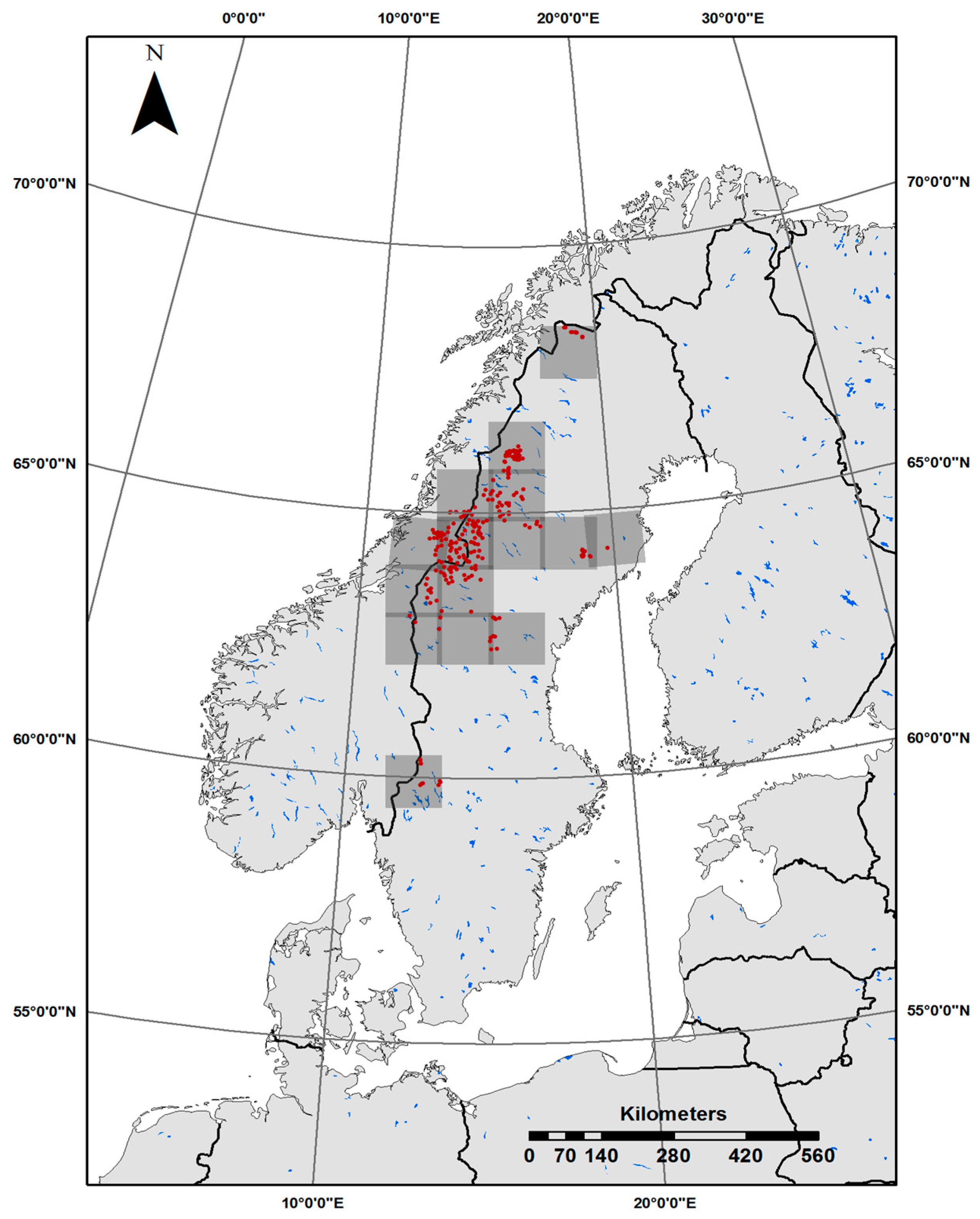
Boreal lakes distributed in Sweden and Norway (Figure 1; n = 255) were selected to evaluate the regulation of lake CDOM across broad environmental gradients. The lakes were randomly selected within the proximity (same Sentinel-2 image tiles) of lakes with CDOM validation data previously published by [7,9,13,24]. Forty-four lakes are located in Nord-Trøndelag in Norway, which has variable land cover with mixed forest, natural grassland, wetlands, moors, and heathland. The remaining 211 lakes are located along a latitudinal gradient with unproductive subarctic landscape in the far north, which consists mainly of birch forest, shrublands, and bare rock, to relatively productive boreal forests in the south. Moreover, there is a general longitudinal gradient with alpine landscapes being increasingly abundant toward the west, in settings spanning from lowland spruce forest to birch forest, shrub-/grasslands, and high alpine conditions. There is no regular monitoring plan for these lakes as they are relatively inaccessible (Figure 1). Human activity in the study area is limited, except forestry in the south. A breakdown of catchment land cover is provided in Table S1.
2.2. Data Compilation and Analyses
2.2.1. Assessment of CDOM Using Remote Sensing
Lake CDOM was assessed for all 255 lakes using a remote sensing methodology that is detailed in Al-Kharusi et al. [26]. In short, Sentinel-2 satellite observations between June and August during 2016 and 2018 were downloaded from the Copernicus Scientific Data Hub (https://scihub.copernicus.eu, accessed 1 December 2020). The effects of the atmosphere, cirrus clouds, and terrain were removed using the Sen2Cor version 2.9.0 module, which resulted in surface reflectance values. We used an algorithm for CDOM retrieval by Al-Kharusi et al. [26], where CDOM is based on the absorbance coefficient expressed in Napierian units at a wavelength of 420 nm, determined from the green (B3; 560 nm) and red (B4; 665 nm) bands of Sentinel-2.
Using Equation (1) (see Table S2 for band definitions), CDOM has previously been predicted (R2 = 0.65) across widespread and diverse regions of Scandinavia [26], including very small lakes that are comparable in size to the smallest lakes in this study. This is a simple model, designed to perform well across a large geographical extent included in this study. The lakes that were used to develop the model (n = 46) are included as a subset of the 255 lakes used in this study, and are evenly distributed among the study lakes to ensure representativeness and accuracy of the model. The fit of the model (R2 = 0.65) is based on 2016 data [26], but is assumed to be similar for 2018, although CDOM ground data unfortunately are lacking for 2018.
2.2.2. Land Cover and Vegetation Index
Catchment land cover data were obtained using the 2012 and 2018 CORINE Land Cover (CLC) dataset provided by the Copernicus Land Monitoring Service (https://land.copernicus.eu/pan-european/corine-land-cover accessed on 15 December 2023). These datasets are an inventory of land cover in 44 classes presented as a cartographic product for most areas of Europe at a scale of 1:100,000. For the normalized difference vegetation index data used, see details in Bianchi et al. [28].
2.2.3. Lake and Catchment Morphometry
A digital elevation model from the Shuttle Radar Topography Mission (SRTM) at a 30 m spatial resolution (downloaded from https://earthexplorer.usgs.gov, 2 April 2020) was used to delineate watersheds. An eight-direction flow matrix (D8) analysis was used for the delineation following a sequence of steps in ArcGIS 10.3.1 that involved a series of neighborhood analysis operations [29]. A set of physical catchment descriptors was applied for the upstream contributing watershed areas following Peters et al. [30].
2.2.4. Climate Data
Monthly average air temperature (°C) and precipitation (mm) from ERA5-Land (https://doi.org/10.24381/cds.68d2bb30, accessed on 15 December 2023) from June to August of 2016 and 2018 were used. The Palmer drought index (PDI) was accessed from June to August for 2016 and 2018 from the Climatic Research Unit (CRU) (https://crudata.uea.ac.uk/cru/data/drought, downloaded on 6 March 2020). The PDI is based on the interpolated fields of monthly precipitation and temperature observations available in the CRU high-resolution surface climate data [31]. The PDI scale indicates drought at negative values, whereas neutral and wet conditions are indicated by zero and positive values, respectively.
2.3. Statistical Analysis
Prior to statistical analysis, the skewness of the data was determined using the PerformanceAnalytics package in R 3.0 (R Core Team, 2018). Variables with Fisher’s skewness values > 2 were natural ln-transformed. This included the variable CDOM, which was positively skewed and needed to be transformed. Averages in PDI and ln(CDOM) between the different years were compared using a paired-sample t-test within R.
2.3.1. Variance Partitioning
Variance partitioning was carried out with CDOM as a response variable and three different matrices with predictor variables in the categories of climate, catchment morphometry, and land cover. The partitioning was carried out using the function varpart from the community ecology package in R called vegan, which performs partitioning by partial regression. Forward model selection was applied until the model could not be improved further. Thus, we performed variance partitioning to assess overlapping predictor values by groups of variables [32,33]. The chosen variables tested in the model are listed in Table 1.
2.3.2. Partial Least-Squares Analysis with Variable Selection
Partial least-squares regression (PLSR) was carried out using the pls package in R. The PLSR was fitted using the O-scores method and cross-validation on scaled data of a set of variables (climate, land cover, and catchment morphometry). The number of components was estimated using the one sigma, randomization, and cross-validation methods using 10 segments. Embedded variable selection was carried out using a powered or sparse PLS [34], with seven components and a thresholding parameter (eta) of 0.8. Using this model, the coefficients of the selected variables (Table 1) were used to show the strength and direction of their relationship with CDOM.
2.3.3. Moran’s Eigenvector Spatial Regression
To overcome potential spatial autocorrelation and to account for spatially varying coefficients (SVCs) for key CDOM predictor variables, random effects eigenvector spatial filtering (RE-ESF) models were fitted using the SP-moran package in R. Variables were pre-selected based on the PLSR variable selection. All possible combinations of variables were modeled for a total of 4095 combinations. The best model was selected based on the Akaike Information Criterion (AIC) and the Bayesian Information Criterion (BIC). To prevent collinearity, we calculated the variable inflation factor (VIF) of the models and only selected models with VIF < 3. A limitation of this analysis is that the study lakes showed an irregular spatial distribution, which makes it difficult to decipher fine spatial structures [35]; hence, the analysis should be seen as an attempt to address the broad spatial patterns only.
3. Results
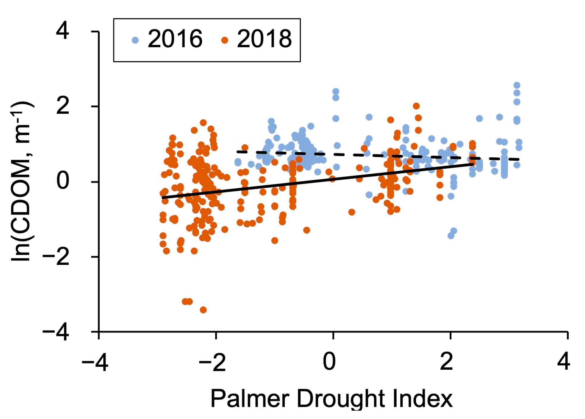
The PDI was lower (p < 0.001; two-tail paired t-test) for the year 2018 compared to 2016, indicating dryer conditions in 2018. The average PDI was 1.68–1.93 (95% confidence interval, CI) units lower in 2018 than in 2016. At the same time, the ln(CDOM) was lower (p < 0.001; two-tail paired t-test) for the dry year of 2018 than for 2016. In the dry year of 2018, a more severe drought was correlated with lower CDOM values (Figure 2). In contrast, during the wet year of 2016, no corresponding correlation was found.
3.1. Regulation of CDOM by Catchment Morphometry, Land Cover, and Climate
3.1.1. Wet Year
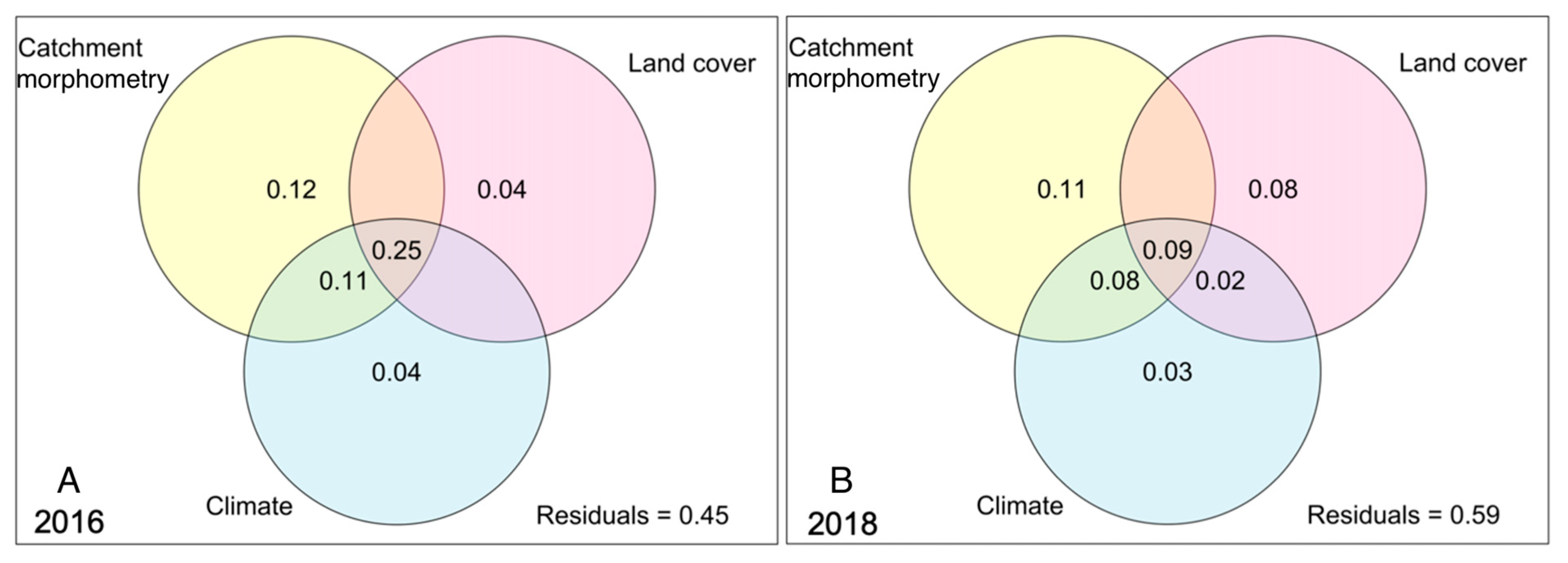
Variables in the three categories “catchment morphometry”, “land cover”, and “climate” together explained a majority of the variation (R2 = 0.55) in CDOM in the wet year of 2016 (Figure 3). The explained variance that was shared, i.e., overlapping, between all three categories was relatively large (R2 = 0.25). Catchment morphometry and climate overlapped in a total of 36% of the explained CDOM variability (shared terms R2 = 0.25 + R2 = 0.11; Figure 3). The uniquely explained variability in CDOM for 2016 was the highest for catchment morphometry (R2 = 0.12), followed by small unique contributions for climate (R2 = 0.04) and land cover (R2 = 0.04) variables.
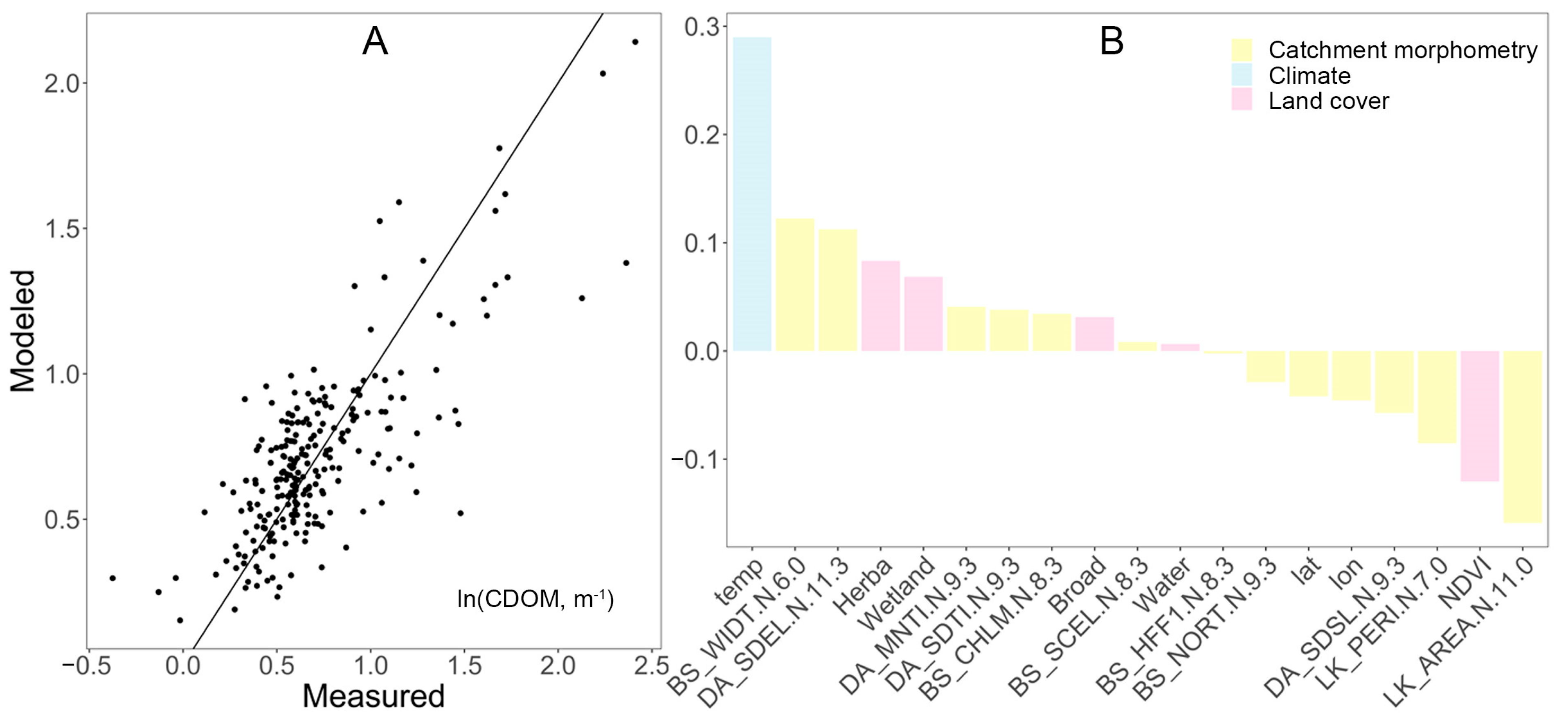
In the PLS model, the predicted versus measured CDOM showed a relatively good fit in the range of ln(CDOM) values between 0.25 to 1, which corresponds to a CDOM range between 1.3 m−1 and 2.7 m−1 (Figure 4). At high and low concentrations, the model slightly under- and overestimated CDOM, respectively. Although the strongest driver of the PLSR model was temperature, variables related to catchment morphometry (e.g., basin width, lake area, and elevation) and land cover (e.g., herbaceous vegetation, wetland, broad leaf forest, water bodies, and mixed forests) also influenced the model of lake CDOM (Figure 4).
3.1.2. Dry Year
The combination of all predictors explained a moderate portion (R2 = 0.19) of the variation in CDOM in 2018 (Figure 3). Moreover, a relatively small amount of explained variability (R2 = 0.09) was shared between all three variable categories. The uniquely explained variability by variable category was highest for catchment morphometry (R2 = 0.11), followed by land cover (R2 = 0.08) and climate, where the climate category alone explained little of the CDOM variation (R2 = 0.03).
Compared with the wet year results, the PLS for the dry year of 2018 showed a less significant fit in terms of modeled versus measured CDOM, and slightly different regulation patterns (Figure 5). Again, climate had a strong effect on CDOM (positive for PDI values and temperature), but catchment morphometry variables (e.g., basin width, lake area, and elevation) also added explanatory value. Land cover was a relatively less important category, with only a few variables of moderate explanatory value (e.g., herbaceous vegetation, wetland, and broad leaf forest). Interestingly, NDVI was a relatively strong negative regulator of CDOM.
3.2. Key Regulators of CDOM in Wet and Dry Years
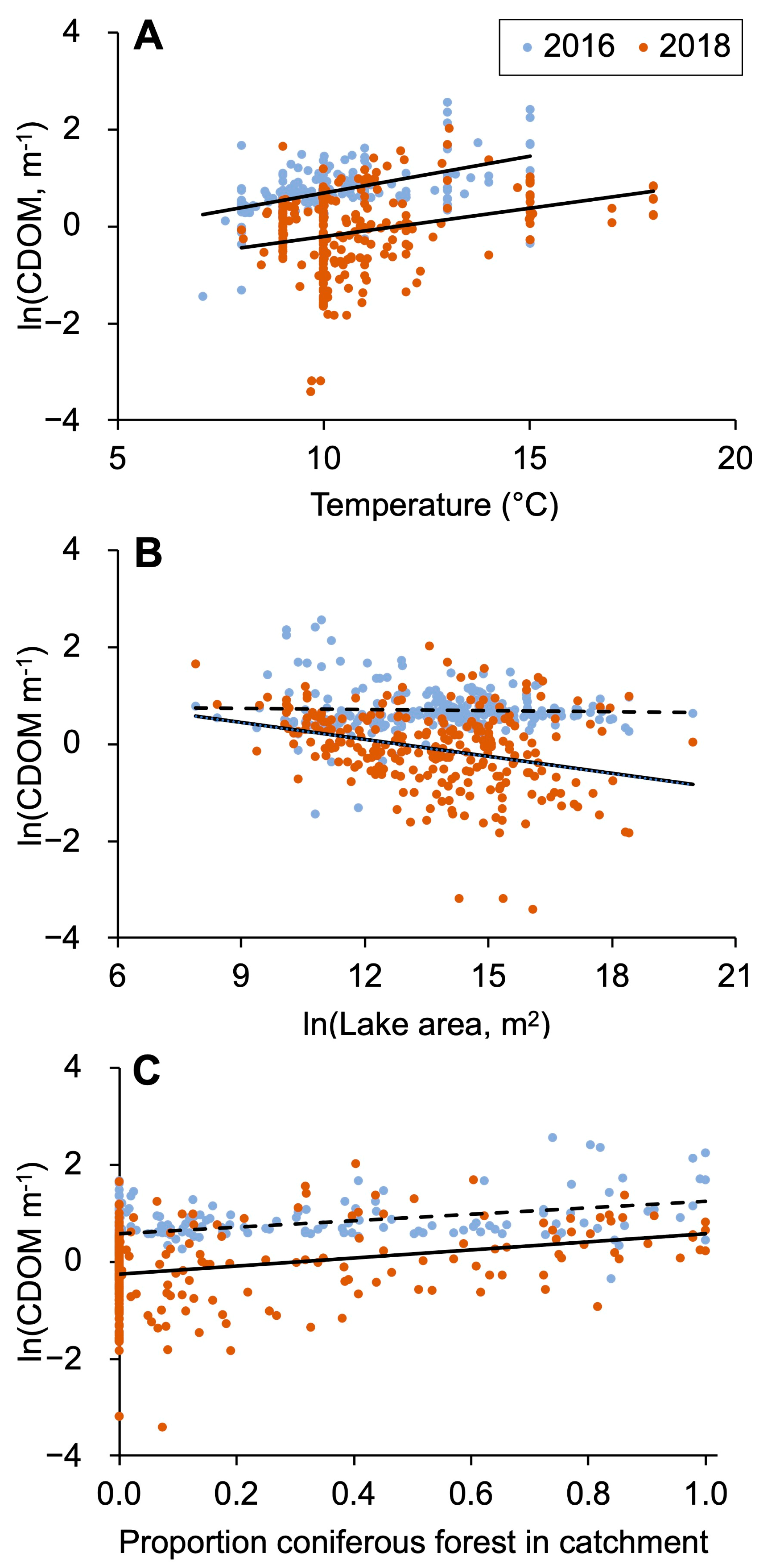
The ln-transformed values of CDOM increased linearly with temperature in both study years (Figure 6A). These relationships showed a similar slope between the years, but the explained variability was relatively lower in the dry year of 2018 when the data were scattered toward lower values. Lake area was one of the most important variables in the PLSR models, however, showing a different degree of importance in the two years. Looking closer at the relationship between CDOM and lake area (Figure 6B), there was a negative correlation between CDOM and lake area in the dry year of 2018, but no such direct relationship was found in the 2016 wet year. This shaped a pattern where small lakes according to the trendlines had similar CDOM concentrations in the two years, whereas large lakes had lower CDOM in the dry year of 2018, compared with the wet year of 2016 (Figure 6B). Surprisingly, the relative abundance of coniferous forest was not an important regulator of CDOM according to the PLSR results. However, there was a moderately strong positive correlation between coniferous forest and CDOM in the wet year of 2016 (Figure 6C). During 2018, this relationship was similar to that in 2016, but not statistically significant.
3.3. Spatial Model for CDOM
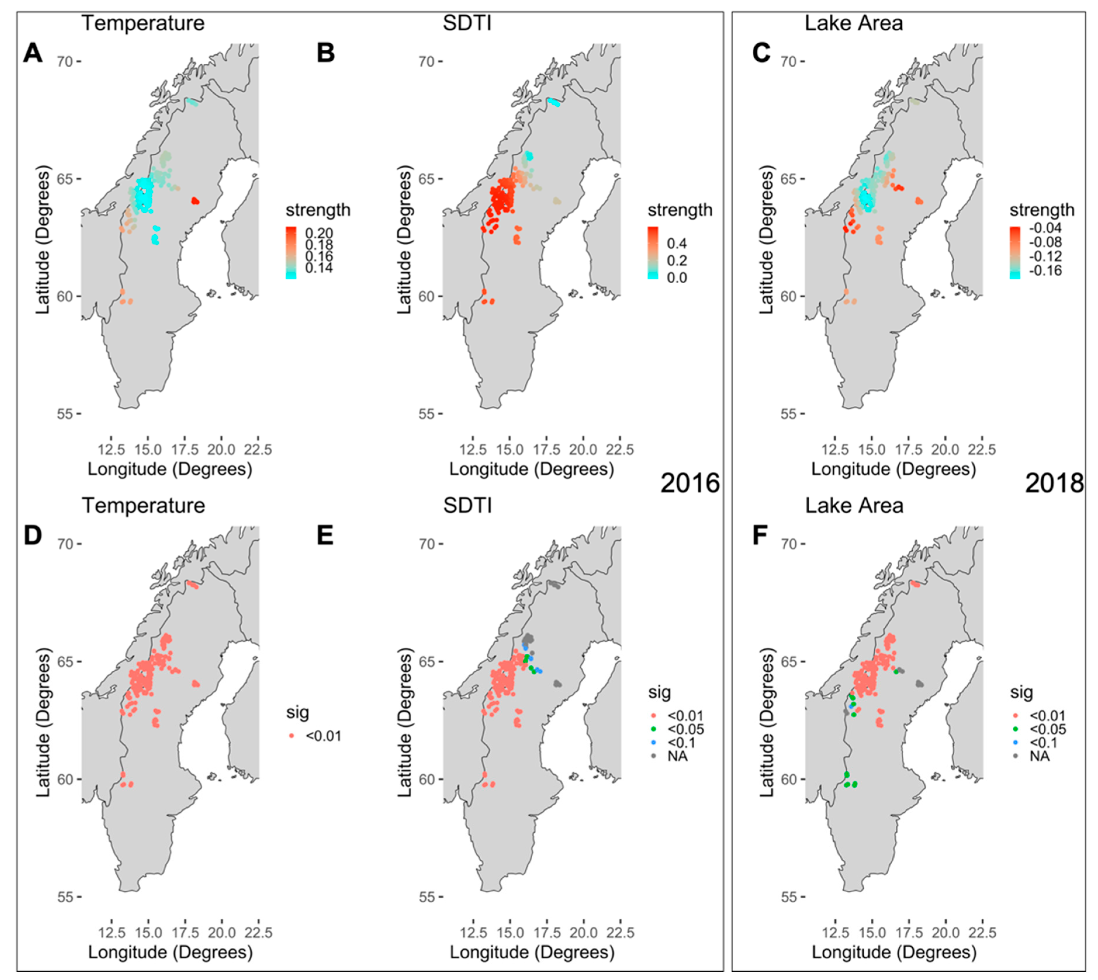
When correcting for spatial auto-correlation using Moran’s eigenvector, only three and two variables were selected for 2016 and 2018, respectively. The final models were able to explain 67% of the variance in CDOM for 2016 and 54% in 2018 (Table 2). In the 2016 wet year, CDOM was driven by the positive effects of temperature and SDTI (drainage area std. dev. topographic index, “DA_SDTI.N.9.3”) (Figure 7A,B). Lake area had a negative effect on CDOM for both years. In addition, the percentage of wetland area had a positive effect in the dry year of 2018. The strength of temperature and SDTI varied spatially, showing a lower effect of SDTI in northern Sweden and a stronger effect of temperature in southern and eastern Sweden in 2016 (Figure 7D,E). Lake area had a relatively small effect in 2016 and did not vary spatially, while, in 2018, it was stronger especially in the northern and areas of Sweden without mountains (Figure 7C,F). The positive effect of the wetland area did not vary spatially in 2018. The intercepts were spatially stable in 2018 (1.29), but increased slightly from towards northern Sweden in 2016, although the difference between points was not significant (Figure S1).
4. Discussion
This study shows how drought can modify the magnitude and regulation of CDOM in lakes on a large scale along broad environmental gradients. Across the study area, the drought of 2018 was associated with significantly decreased CDOM compared to the wet year of 2016, and this effect on CDOM was linked to the severity of drought. However, contrary to our hypothesis, climate variables (especially temperature) played a smaller role in CDOM regulation during the dry year, compared to the wet year. Using multiple statistical approaches, we show that CDOM variations during drought are relatively difficult to predict, implying that drought not only offsets CDOM toward lower values, but also weakens its regulation by a wide range of factors. Below, we discuss the effects climate, land cover, and morphometry drivers have on the patterns of lake CDOM during both dry and wet conditions, and their implications in the context of climate change.
4.1. Direct Impact of Drought on CDOM
During the dry year of 2018, the degree of drought (more negative Palmer drought index; PDI) caused decreased lake CDOM, while no significant direct impact from the PDI was observed during the wet year 2016. This suggests that variations in the PDI do not generically regulate CDOM, but rather it is the anomaly in the PDI during an unusually dry period that affects CDOM. This finding agrees with previous results pointing to disrupted linkages between lake waters and catchments during periods of drought [36], resulting from a sequential decline in precipitation, soil moisture, groundwater levels, runoff, and streamflow [37]. During such periods, there can be an increased extent and duration of algal blooms in the lakes due to the heat [38], but the DOM from algae is transparent and contributes relatively little to CDOM [39], especially in relation to the high rates of the photochemical removal of CDOM in light-exposed stagnant lake waters [19]. Thus, CDOM input is limited by upstream terrestrial sources, through streams that are connected hydrologically with riparian zones and vertically with the hyporheic zone and shallow groundwater [40]. However, in severe drought cases, the streams can partly dry out [41] which hinders the surface water movement and delivery of materials to the lake water [36,40]. Additionally, during drought, a larger part of the hydrological input to lakes may be in the form of deeper groundwater that is known to dilute DOM [21]. In this way, water bodies can be disconnected from their surroundings with reduced water flow, with a variety of consequences for water quality and habitats [36].
Drought has a major impact on terrestrial microbial activity, with wide-ranging impacts on carbon and nutrient cycling, and plant production [42]. Low soil moisture can stress micro-organisms and restrict key enzymes involved in soil organic matter processing and the leaching of DOM from plant litter [43,44], thus decreasing the potential for the production and export of CDOM from soils to streams. Additionally, summer drought has been found to reduce photosynthetic plant rates and carbon allocation from plants, roots to soil [3,45,46]. Changes in the flow of carbon from plants to the soil can be influenced by the depletion of the nutrient supply during dry periods to the soil microbial community, particularly mycorrhizal species [36,47]. This suggests that less fresh terrestrial organic matter sources from catchment vegetation and soils are available for export to recipient freshwaters. Thus, drought may not only limit the hydrological delivery of DOM and CDOM to lakes, but it can also decrease the production of DOM within the catchment itself, which helps explain why lake CDOM was much lower during the year of the drought, particularly in the areas with the most severe impact.
4.2. Shifts in the Relative Importance of Climate, Land Cover, and Morphometry
The variance partitioning results did not support the hypothesized shift from land cover control during wet conditions to climate control during drought. Instead, the variance explained by all variable categories except land cover decreased from the wet year to the dry year. A possible interpretation of this is that the catchment influence on lake CDOM is more strongly expressed during wet conditions, when lakes are relatively more hydrologically connected to their surroundings. The importance of temperature on CDOM mobilization from the catchment agrees with past findings of temperature-driven increases in the production of soil carbon and transfer of carbon to boreal lakes [24,48]. Moreover, direct runoff has a more significant impact on a lake’s CDOM concentration than the input of groundwater, which is relatively more important during dryer periods [2]. At the same time, climatic effects on the internal turnover of CDOM in the lakes may not have been of major importance, since the temperature-dependent microbial degradation often does not remove any larger fraction of the DOM during its transit through boreal lakes, although this may vary with water residence times [19,49]. Thus, our results stress the importance of wet conditions for the controls of climate, land cover, and morphometry on CDOM.
The total land cover influence on CDOM decreased as expected from the wet to the dry year, but, unexpectedly, the variance partitioning showed that land cover explained the slightly more unique CDOM variability during dry conditions. A possible explanation for this is that different land cover types suffer to different degrees with regard to the loss of hydrological connectivity to recipients during drought. For example, a high accumulation of soil organic carbon occurs in wetlands catchments which have large water reserves and can export even greater DOM concentrations during base flow [48]. In our case, wetlands had a substantial influence on the Moran’s model results specifically during dry conditions, suggesting that lakes do not easily become hydrologically uncoupled from wetlands.
4.3. Controls of CDOM Evaluated Using PLS and Moran’s Eigenvector Spatial Model
In the wet year, temperature played an overwhelmingly important role as a CDOM regulator, exceeding its importance during the dry year. This result is in opposition to our hypothesis that climate variables are relatively more important during drought, e.g., due to accelerated internal microbial DOM degradation in the water [50]. Interestingly, our results showed a systematically positive temperature effect on CDOM, implying that the increased delivery of CDOM to the lakes at higher temperatures was more important than the temperature-stimulated CDOM degradation leading to internal losses in the lakes. The fact that this pattern was the strongest during the wet year agrees with previous results from catchments in northern Sweden, showing that the combination of warm and wet summers can yield exceptionally high DOM exports from both forests and wetlands [51]. Moreover, it has been found that DOM in boreal soil increase rapidly in response to higher temperature [52], and that the increasing temperature and precipitation increase CDOM in freshwaters [3]. Thus, whereas drought is a negative CDOM regulator, the regulation of CDOM by temperature in the region appears to be systematically positive, yet particularly pronounced during wet years.
Land cover variables had a significant impact on CDOM in both years, especially through herbaceous vegetation, mixed forest, and wetland, which agrees with many previous studies [2,17,53]. However, in the PLSR results, both NDVI and the abundance of coniferous forest were negative CDOM regulators, which is in disagreement with past research that found these variables to be key positive regulators of DOM [27,53]. These surprising results may partly be due to the PLSR method itself, since it shows the relative influence of each variable when taking the influence of all other variables into account. Nonetheless, the strong negative influence from NDVI on CDOM is remarkable in relation to previous findings [53,54], and questions the usefulness of NDVI as a coherent indicator of CDOM. Patterns in NDVI are related to the land cover type, and, given that each land cover type has its own distinct relationship between productivity and NDVI [55], it is possible that the results are biased. For example, coniferous forests with a high CDOM export usually have low NDVI values, while unproductive sparse mountain birch forests can have high NDVI values in spite of being associated with a low DOM export [55,56]. Thus, it is possible that the high NDVI did not reflect the high CDOM in this study, because high DOM can be found for land cover types where NDVI is inherently low, including wetlands [20].
Lake area was the most important morphometry variable in this study, being negatively related to CDOM, which agrees with past findings. For example, Mattsson et al. [57] concluded that lake area is the critical variable for decreasing organic carbon in Finnish catchments, and Arvola et al. [9] emphasized that lake area leads to decreased CDOM and has a stronger impact than catchment wetlands. An interpretation of this result is that small lakes remained connected to catchment CDOM sources during the drought, while the bigger lakes lost hydrological connectivity whereby CDOM underwent bacterial breakdown/and or photo-bleaching [19] without being replenished. In this regard, the position of the lakes in the landscape is crucial, because the small lakes are relatively closer to the terrestrial sources of CDOM than the larger lakes, which are often located further down in the catchment and fed by deeper groundwater.
Although considered as three separate groups of explanatory variables, the variation in land cover, climate, and morphometry variables are likely inter-related, complicating the interpretation of the results. For instance, temperature is known to have a positive effect on vegetation production and NDVI during summer [58], making it difficult to disentangle the vegetation effect from the temperature effect on CDOM, although our results highlight temperature as the chief regulator. Similarly, inter-relations between morphometry and land cover may have affected our results. In the wet year, a higher standard deviation in the topographic wetness index leads to greater CDOM concentrations potentially because the catchments with a more variable topographic index have both abundant wetlands and catchment sections with steeper slopes that efficiently transport the wetland-derived CDOM into lakes [54]. During the dry year, SDTI did not affect the lake CDOM. However, wetlands, which retain greater connectivity even during extreme droughts, did have a positive effect on CDOM, according to Moran’s model results also in the dry year.
4.4. CDOM in Changing Climate
This study shows how climate warming can positively affect lake CDOM concentrations during a wet year. However, increased drought can temporarily decrease values as upland carbon sources are temporarily disconnected from the hydrological system [36]. Thus, similar to what was observed for Minnesota lakes by Olmanson et al. [59], we found that regional CDOM was lower in a dry compared to a wet year. When a wet period follows a dry period, CDOM could quickly increase again and even become higher than it was before the dry period [60]. Thus, climate changes can result in a combination of changes in hydrology, vegetation type, and productivity that lead to greater intra-annual variations in the CDOM of recipient waters. The projected future climate, with more extreme alternations between dry and wet periods, will likely cause an increasing variability in CDOM, which, in turn, may result in major and nonlinear changes in important lake ecosystem functions such as gross primary production and fish biomass [61,62,63,64]. As some lakes are the main potable water sources for residents, this might lead to greater costs for drinking water treatment since large variations in CDOM implies a need to implement different treatment protocols to improve the water quality [65].
4.5. Study Robustness
Using remote sensing and geographic information systems to retrieve lake CDOM and catchment characteristics, respectively, are efficient techniques for addressing their relationships at a large scale. However, cloud conditions in the dry and largely clear-sky summer of 2018 were more favorable for remote sensing compared with the cloudy year of 2016. Nonetheless, despite the risk of more atmospheric interference in 2016, we were able to build the relatively strongest models of CDOM prediction during this year, implying that our analyses had sufficient resolution to see the declines and changes in catchment, morphometry, and climate controls on CDOM that were brought by the drought. We were also able to accurately detect the trend of decreasing mean CDOM from 2016 to 2018, which agrees with the general pattern of decreasing mean absorbance at 420 nm from the wet year 2016 to the dry year 2018 in the national monitoring of lakes of the involved regions (data source; https://miljodata.slu.se/MVM/Search accessed on 15 December 2023).
5. Conclusions
In broadly distributed lakes across large parts of Sweden, we found that severe drought strongly decreased CDOM during a dry year, during which a significant correlation was found between drought intensity and CDOM. Large lakes showed particularly low CDOM during the dry year, presumably due to a high degree of catchment uncoupling. Although we hypothesized shifts in the importance of different types of regulation of CDOM depending on drought intensity, we found that all studied variable categories—climate, land cover, and morphometry—had a stronger impact on CDOM in the wet vs. dry year. Thus, drought systematically weakened the regulation of CDOM at the same time that CDOM was offset toward lower values. In a future climate with higher frequencies of both extremely dry and wet periods, considerable temporal variations in CDOM are expected.
Supplementary Materials
The following supporting information can be downloaded at https://www.mdpi.com/article/10.3390/rs16081345/s1. Table S1: Percentage of land cover in the cumulative area of the study catchments; Table S2: Resolution, radiometry and signal-to-noise ratio (SNR) of Sentinel-2 bands; Table S3: Variation partitioning sub-datasets [30]; Figure S1: The spatial coefficient of variation (SCV) of temperature and lake area.
Author Contributions
Conceptualization, M.B. and E.S.A.-K.; methodology, G.H., E.S.A.-K., T.K., D.E.T. and A.M.A.; formal analysis, E.S.A.-K. and G.H.; investigation, M.B.; resources, M.B. and J.K.; writing—original draft preparation, M.B. and E.S.A.-K.; writing—review and editing, all authors; visualization, E.S.A.-K. and G.H.; supervision, M.B. and D.E.T. All authors have read and agreed to the published version of the manuscript.
Funding
We thank the Royal Physiographic Society of Lund, Sweden (Grant No. 161116) for supporting this study. E. S. Al-Kharusi was further supported by the Ministry of Higher Education, National programme of postgraduate studies, Sultanate of Oman. A. M. Abdi was supported by the Swedish Research Council (Grant No. 2018-00430). Finally, M. Berggren was supported by FORMAS (Grant No. 2017-00772) and the Swedish Research Council VR (Grant No. 2018-04111).
Data Availability Statement
All the data are available in public repositories, as explained in the paper.
Conflicts of Interest
The authors declare there are no conflicts of interest.
References
- Brezonik, P.L.; Olmanson, L.G.; Finlay, J.C.; Bauer, M.E. Factors affecting the measurement of CDOM by remote sensing of optically complex inland waters. Remote Sens. Environ. 2015, 157, 199–215. [Google Scholar] [CrossRef]
- Sobek, S.; Algesten, G.; Bergström, A.K.; Jansson, M.; Tranvik, L.J. The catchment and climate regulation of pCO2 in boreal lakes. Glob. Chang. Biol. 2003, 9, 630–641. [Google Scholar] [CrossRef]
- Kritzberg, E.S.; Hasselquist, E.M.; Skerlep, M.; Löfgren, S.; Olsson, O.; Stadmark, J.; Valinia, S.; Hansson, L.A.; Laudon, H. Browning of freshwaters: Consequences to ecosystem services, underlying drivers, and potential mitigation measures. Ambio 2020, 49, 375–390. [Google Scholar] [CrossRef] [PubMed]
- Keeler, B.L.; Wood, S.A.; Polasky, S.; Kling, C.; Filstrup, C.T.; Downing, J.A. Recreational demand for clean water: Evidence from geotagged photographs by visitors to lakes. Front. Ecol. Environ. 2015, 13, 76–81. [Google Scholar] [CrossRef] [PubMed]
- Skerlep, M.; Steiner, E.; Axelsson, A.L.; Kritzberg, E.S. Afforestation driving long-term surface water browning. Glob. Chang. Biol. 2020, 26, 1390–1399. [Google Scholar] [CrossRef] [PubMed]
- Jaffé, R.; McKnight, D.; Maie, N.; Cory, R.; McDowell, W.H.; Campbell, J.L. Spatial and temporal variations in DOM composition in ecosystems: The importance of long-term monitoring of optical properties. J. Geophys. Res. Biogeosci. 2008, 113, G04032. [Google Scholar] [CrossRef]
- Yao, X.; Zhang, Y.L.; Zhu, G.W.; Qin, B.Q.; Feng, L.Q.; Cai, L.L.; Gao, G.A. Resolving the variability of CDOM fluorescence to differentiate the sources and fate of DOM in Lake Taihu and its tributaries. Chemosphere 2011, 82, 145–155. [Google Scholar] [CrossRef] [PubMed]
- Jacome, A.; Bernier, M.; Chokmani, K.; Gauthier, Y.; Poulin, J.; De Sève, D. Monitoring volumetric surface soil moisture content at the La Grande basin boreal wetland by radar multi polarization data. Remote Sens. 2013, 5, 4919–4941. [Google Scholar] [CrossRef]
- Arvola, L.; Aijala, C.; Lepparanta, M. CDOM concentrations of large Finnish lakes relative to their landscape properties. Hydrobiologia 2016, 780, 37–46. [Google Scholar] [CrossRef]
- Barnes, R.T.; Butman, D.E.; Wilson, H.F.; Raymond, P.A. Riverine export of aged carbon driven by flow path depth and residence time. Environ. Sci. Technol. 2018, 52, 1028–1035. [Google Scholar] [CrossRef] [PubMed]
- Wickland, K.P.; Neff, J.C.; Aiken, G.R. Dissolved organic carbon in Alaskan boreal forest: Sources, chemical characteristics, and biodegradability. Ecosystems 2007, 10, 1323–1340. [Google Scholar] [CrossRef]
- Kallio, K.; Attila, J.; Härmä, P.; Koponen, S.; Pulliainen, J.; Hyytiäinen, U.M.; Pyhälahti, T. Landsat ETM+ images in the estimation of seasonal lake water quality in boreal river basins. Environ. Manag. 2008, 42, 511–522. [Google Scholar] [CrossRef] [PubMed]
- Larsen, S.; Andersen, T.; Hessen, D.O. Climate change predicted to cause severe increase of organic carbon in lakes. Glob. Chang. Biol. 2011, 17, 1186–1192. [Google Scholar] [CrossRef]
- Treat, C.C.; Marushchak, M.E.; Voigt, C.; Zhang, Y.; Tan, Z.L.; Zhuang, Q.L.; Virtanen, T.A.; Räsänen, A.; Biasi, C.; Hugelius, G.; et al. Tundra landscape heterogeneity, not interannual variability, controls the decadal regional carbon balance in the Western Russian Arctic. Glob. Chang. Biol. 2018, 24, 5188–5204. [Google Scholar] [CrossRef] [PubMed]
- Laudon, H.; Berggren, M.; Ågren, A.; Buffam, I.; Bishop, K.; Grabs, T.; Jansson, M.; Köhler, S. Patterns and dynamics of dissolved organic carbon (DOC) in boreal streams: The role of processes, connectivity, and scaling. Ecosystems 2011, 14, 880–893. [Google Scholar] [CrossRef]
- Bodmer, P.; Heinz, M.; Pusch, M.; Singer, G.; Premke, K. Carbon dynamics and their link to dissolved organic matter quality across contrasting stream ecosystems. Sci. Total Environ. 2016, 553, 574–586. [Google Scholar] [CrossRef]
- Hutchins, R.H.S.; Prairie, Y.T.; del Giorgio, P.A. Large-scale landscape drivers of CO2, CH4, DOC, and DIC in boreal river networks. Glob. Biogeochem. Cycles 2019, 33, 125–142. [Google Scholar] [CrossRef]
- Jordan, Y.C.; Ghulam, A.; Hartling, S. Traits of surface water pollution under climate and land use changes: A remote sensing and hydrological modeling approach. Earth Sci. Rev. 2014, 128, 181–195. [Google Scholar] [CrossRef]
- Berggren, M.; Klaus, M.; Selvam, B.P.; Strom, L.; Laudon, H.; Jansson, M.; Karlsson, J. Quality transformation of dissolved organic carbon during water transit through lakes: Contrasting controls by photochemical and biological processes. Biogeosciences 2018, 15, 457–470. [Google Scholar] [CrossRef]
- Mzobe, P.; Berggren, M.; Pilesjö, P.; Lundin, E.; Olefeldt, D.; Roulet, N.T.; Persson, A. Dissolved organic carbon in streams within a subarctic catchment analysed using a GIS/remote sensing approach. PLoS ONE 2018, 13, e0199608. [Google Scholar] [CrossRef] [PubMed]
- Tiwari, T.; Buffam, I.; Sponseller, R.A.; Laudon, H. Inferring scale-dependent processes influencing stream water biogeochemistry from headwater to sea. Limnol. Oceanogr. 2017, 62, S58–S70. [Google Scholar] [CrossRef]
- Toming, K.; Arst, H.; Paavel, B.; Laas, A.; Noges, T. Spatial and temporal variations in coloured dissolved organic matter in large and shallow Estonian waterbodies. Boreal. Environ. Res. 2009, 14, 959–970. [Google Scholar]
- Zhang, Y.L.; Yin, Y.; Liu, X.H.; Shi, Z.Q.; Feng, L.Q.; Liu, M.L.; Zhu, G.W.; Gong, Z.J.; Qin, B.Q. Spatial-seasonal dynamics of chromophoric dissolved organic matter in Lake Taihu, a large eutrophic, shallow lake in China. Org. Geochem. 2011, 42, 510–519. [Google Scholar] [CrossRef]
- Lapierre, J.F.; Seekell, D.A.; del Giorgio, P.A. Climate and landscape influence on indicators of lake carbon cycling through spatial patterns in dissolved organic carbon. Glob. Chang. Biol. 2015, 21, 4425–4435. [Google Scholar] [CrossRef] [PubMed]
- Klaus, M.; Seekell, D.A.; Lidberg, W.; Karlsson, J. Evaluations of climate and land management effects on lake carbon cycling need to account temporal variability in CO<sub>2</sub> Concentration. Glob. Biogeochem. Cycles 2019, 33, 243–265. [Google Scholar] [CrossRef]
- Al-Kharusi, E.S.; Tenenbaum, D.E.; Abdi, A.M.; Kutser, T.; Karlsson, J.; Bergström, A.K.; Berggren, M. Large-scale retrieval of coloured dissolved organic matter in northern lakes using Sentinel-2 data. Remote Sens. 2020, 12, 157. [Google Scholar] [CrossRef]
- Jansson, M.; Hickler, T.; Jonsson, A.; Karlsson, J. Links between terrestrial primary production and bacterial production and respiration in lakes in a climate gradient in subarctic Sweden. Ecosystems 2008, 11, 367–376. [Google Scholar] [CrossRef]
- Bianchi, E.; Villalba, R.; Solarte, A. NDVI Spatio-temporal Patterns and Climatic Controls Over Northern Patagonia. Ecosystems 2020, 23, 84–97. [Google Scholar] [CrossRef]
- Turcotte, R.; Fortin, J.P.; Rousseau, A.N.; Massicotte, S.; Villeneuve, J.P. Determination of the drainage structure of a watershed using a digital elevation model and a digital river and lake network. J. Hydrol. 2001, 240, 225–242. [Google Scholar] [CrossRef]
- Peters, D.L.; Baird, D.J.; Tenenbaum, D.E. Towards the Development of Instream Flow Needs Standards for Agricultural Watersheds in Canada—2006/07 Interim Report; Environmental Standards Initiative Technical Series Report No. 3–40; Environment Canada: Gatineau, QB, Canada, 2007; p. 89. [Google Scholar]
- Harris, I.; Jones, P.D.; Osborn, T.J.; Lister, D.H. Updated high-resolution grids of monthly climatic observations—The CRU TS3.10 Dataset. Int. J. Clim. 2014, 34, 623–642. [Google Scholar] [CrossRef]
- Browne, W.J.; Subramanian, S.V.; Jones, K.; Goldstein, H. Variance partitioning in multilevel logistic models that exhibit overdispersion. J. R. Stat. Soc. Ser. A Stat. Soc. 2005, 168, 599–613. [Google Scholar] [CrossRef]
- Peres-Neto, P.R.; Legendre, P.; Dray, S.; Borcard, D. Variation partitioning of species data matrices: Estimation and comparison of fractions. Ecology 2006, 87, 2614–2625. [Google Scholar] [CrossRef] [PubMed]
- Mehmood, T.; Liland, K.H.; Snipen, L.; Sæbo, S. A review of variable selection methods in Partial Least Squares Regression. Chemom. Intell. Lab. Syst. 2012, 118, 62–69. [Google Scholar] [CrossRef]
- Brind’Amour, A.; Mahévas, S.; Legendre, P.; Bellanger, L. Application of Moran Eigenvector Maps (MEM) to irregular sampling designs. Spat. Stat. 2018, 26, 56–68. [Google Scholar] [CrossRef]
- Szkokan-Emilson, E.J.; Kielstra, B.W.; Arnott, S.E.; Watmough, S.A.; Gunn, J.M.; Tanentzap, A.J. Dry conditions disrupt terrestrial-aquatic linkages in northern catchments. Glob. Chang. Biol. 2017, 23, 117–126. [Google Scholar] [CrossRef] [PubMed]
- Hughes, J.D.; Petrone, K.C.; Silberstein, R.P. Drought, groundwater storage and stream flow decline in southwestern Australia. Geophys. Res. Lett. 2012, 39, L03408. [Google Scholar] [CrossRef]
- Wiley, D.Y.; McPherson, R.A. The role of climate change in the proliferation of freshwater harmful algal blooms in inland water bodies of the United States. Earth Interact. 2024, 28, e230008. [Google Scholar] [CrossRef]
- Berggren, M.; Gudasz, C.; Guillemette, F.; Hensgens, G.; Ye, L.; Karlsson, J. Systematic microbial production of optically active dissolved organic matter in subarctic lake water. Limnol. Oceanogr. 2020, 65, 951–961. [Google Scholar] [CrossRef]
- Lake, P.S. Ecological effects of perturbation by drought in flowing waters. Freshw. Biol. 2003, 48, 1161–1172. [Google Scholar] [CrossRef]
- Vazquez, E.; Amalfitano, S.; Fazi, S.; Butturini, A. Dissolved organic matter composition in a fragmented Mediterranean fluvial system under severe drought conditions. Biogeochemistry 2011, 102, 59–72. [Google Scholar] [CrossRef]
- Xiao, W.; Chen, X.; Jing, X.; Zhu, B.A. A meta-analysis of soil extracellular enzyme activities in response to global change. Soil. Biol. Biochem. 2018, 123, 21–32. [Google Scholar] [CrossRef]
- Toberman, H.; Evans, C.D.; Freeman, C.; Fenner, N.; White, M.; Emmett, B.A.; Artz, R.R.E. Summer drought effects upon soil and litter extracellular phenol oxidase activity and soluble carbon release in an upland Calluna heathland. Soil. Biol. Biochem. 2008, 40, 1519–1532. [Google Scholar] [CrossRef]
- Wu, X.Q.; Wu, L.Y.; Liu, Y.; Zhang, P.; Li, Q.H.; Zhou, J.Z.; Hess, N.J.; Hazen, T.C.; Yang, W.L.; Chakraborty, R. Microbial interactions with dissolved organic matter drive carbon dynamics and community succession. Front. Microbiol. 2018, 9, 1234. [Google Scholar] [CrossRef] [PubMed]
- Nemergut, D.R.; Costello, E.K.; Meyer, A.F.; Pescador, M.Y.; Weintraub, M.N.; Schmidt, S.K. Structure and function of alpine and arctic soil microbial communities. Res. Microbiol. 2005, 156, 775–784. [Google Scholar] [CrossRef] [PubMed]
- Breeuwer, A.; Robroek, B.J.M.; Limpens, J.; Heijmans, M.; Schouten, M.G.C.; Berendse, F. Decreased summer water table depth affects peatland vegetation. Basic. Appl. Ecol. 2009, 10, 330–339. [Google Scholar] [CrossRef]
- Ji, M.Y.; Zhou, L.; Zhang, S.C.; Luo, G.; Sang, W.J. Effects of biochar on methane emission from paddy soil: Focusing on DOM and microbial communities. Sci. Total Environ. 2020, 743, 140725. [Google Scholar] [CrossRef] [PubMed]
- Laudon, H.; Buttle, J.; Carey, S.K.; McDonnell, J.; McGuire, K.; Seibert, J.; Shanley, J.; Soulsby, C.; Tetzlaff, D. Cross-regional prediction of long-term trajectory of stream water DOC response to climate change. Geophys. Res. Lett. 2012, 39, L18404. [Google Scholar] [CrossRef]
- Jonsson, A.; Meili, M.; Bergström, A.K.; Jansson, M. Whole-lake mineralization of allochthonous and autochthonous organic carbon in a large humic lake (Örtrasket, N. Sweden). Limnol. Oceanogr. 2001, 46, 1691–1700. [Google Scholar] [CrossRef]
- Berggren, M.; Laudon, H.; Jonsson, A.; Jansson, M. Nutrient constraints on metabolism affect the temperature regulation of aquatic bacterial growth efficiency. Microb. Ecol. 2010, 60, 894–902. [Google Scholar] [CrossRef]
- Köhler, S.J.; Buffam, I.; Laudon, H.; Bishop, K.H. Climate’s control of intra-annual and interannual variability of total organic carbon concentration and flux in two contrasting boreal landscape elements. J. Geophys. Res. Biogeosci. 2008, 113, G03012. [Google Scholar] [CrossRef]
- O’Donnell, J.A.; Aiken, G.R.; Butler, K.D.; Guillemette, F.; Podgorski, D.C.; Spencer, R.G.M. DOM composition and transformation in boreal forest soils: The effects of temperature and organic-horizon decomposition state. J. Geophys. Res. Biogeosci. 2016, 121, 2727–2744. [Google Scholar] [CrossRef]
- Larsen, S.; Andersen, T.; Hessen, D.O. Predicting organic carbon in lakes from climate drivers and catchment properties. Glob. Biogeochem. Cycles 2011, 25, GB3007. [Google Scholar] [CrossRef]
- Mzobe, P.; Yan, Y.; Berggren, M.; Pilesjö, P.; Olefeldt, D.; Lundin, E.; Roulet, N.T.; Persson, A. Morphometric control on dissolved organic carbon in subarctic streams. J. Geophys. Res. Biogeosci. 2020, 125, e2019JG005348. [Google Scholar] [CrossRef]
- Spadoni, G.L.; Cavalli, A.; Congedo, L.; Munafò, M. Analysis of Normalized Difference Vegetation Index (NDVI) multi-temporal series for the production of forest cartography. Remote Sens. Appl. Soc. Environ. 2020, 20, 100419. [Google Scholar] [CrossRef]
- Fiore, N.M.; Goulden, M.L.; Czimczik, C.I.; Pedron, S.A.; Tayo, M.A. Do recent NDVI trends demonstrate boreal forest decline in Alaska? Environ. Res. Lett. 2020, 15, 095007. [Google Scholar] [CrossRef]
- Mattsson, T.; Kortelainen, P.; Raike, A. Export of DOM from boreal catchments: Impacts of land use cover and climate. Biogeochemistry 2005, 76, 373–394. [Google Scholar] [CrossRef]
- Kaufmann, R.K.; Zhou, L.; Myneni, R.B.; Tucker, C.J.; Slayback, D.; Shabanov, N.V.; Pinzon, J. The effect of vegetation on surface temperature: A statistical analysis of NDVI and climate data. Geophys. Res. Lett. 2003, 30, 2147. [Google Scholar] [CrossRef]
- Olmanson, L.G.; Page, B.P.; Finlay, J.C.; Brezonik, P.L.; Bauer, M.E.; Griffin, C.G.; Hozalski, R.M. Regional measurements and spatial/temporal analysis of CDOM in 10,000+optically variable Minnesota lakes using Landsat 8 imagery. Sci. Total Environ. 2020, 724, 138141. [Google Scholar] [CrossRef] [PubMed]
- Tank, S.E.; Fellman, J.B.; Hood, E.; Kritzberg, E.S. Beyond respiration: Controls on lateral carbon fluxes across the terrestrial-aquatic interface. Limnol. Oceanogr. Lett. 2018, 3, 76–88. [Google Scholar] [CrossRef]
- Karlsson, J.; Bergström, A.K.; Byström, P.; Gudasz, C.; Rodriguez, P.; Hein, C. Terrestrial organic matter input suppresses biomass production in lake ecosystems. Ecology 2015, 96, 2870–2876. [Google Scholar] [CrossRef]
- Bergström, A.K.; Karlsson, J. Light and nutrient control phytoplankton biomass responses to global change in northern lakes. Glob. Chang. Biol. 2019, 25, 2021–2029. [Google Scholar] [CrossRef]
- Kelly, P.T.; Solomon, C.T.; Zwart, J.A.; Jones, S.E. A framework for understanding variation in pelagic gross primary production of lake ecosystems. Ecosystems 2018, 21, 1364–1376. [Google Scholar] [CrossRef]
- Vasconcelos, F.R.; Diehl, S.; Rodriguez, P.; Hedström, P.; Karlsson, J.; Byström, P. Bottom-up and top-down effects of browning and warming on shallow lake food webs. Glob. Chang. Biol. 2019, 25, 504–521. [Google Scholar] [CrossRef] [PubMed]
- Chen, Y.L.; Arnold, W.A.; Griffin, C.G.; Olmanson, L.G.; Brezonik, P.L.; Hozalski, R.M. Assessment of the chlorine demand and disinfection byproduct formation potential of surface waters via satellite remote sensing. Water Res. 2019, 165, 115001. [Google Scholar] [CrossRef] [PubMed]
Figure 1.
Locations of the study sites in Sweden and Norway. Sentinel-2 image tiles are highlighted in gray.
Figure 1.
Locations of the study sites in Sweden and Norway. Sentinel-2 image tiles are highlighted in gray.

Figure 2.
Relationship between ln-transformed CDOM (m−1) and Palmer drought index (y = 0.1677x + 0.0652; R2 = 0.11; n = 255; 2-tail p < 0.0001) for all regions in the dry summer season of 2018 (solid line). In the wet year of 2016, there was no significant correlation, hence a dashed line showing the average value. Note that nearby lakes can have identical PDI values due to the course spatial resolution of the downloaded PDI data.

Figure 3.
Variance partitioning of ln(CDOM) for the categories of catchment morphometry, land cover, and climate (16, 11, and 3 variables, respectively) shown for (A) 2016 and (B) 2018 (see list of variables in Table S3). Total adjusted R2 is 0.55 for 2016 and 0.41 for 2018. Partitioning of adjusted R2 is shown in the graph. Insignificant values are not shown.

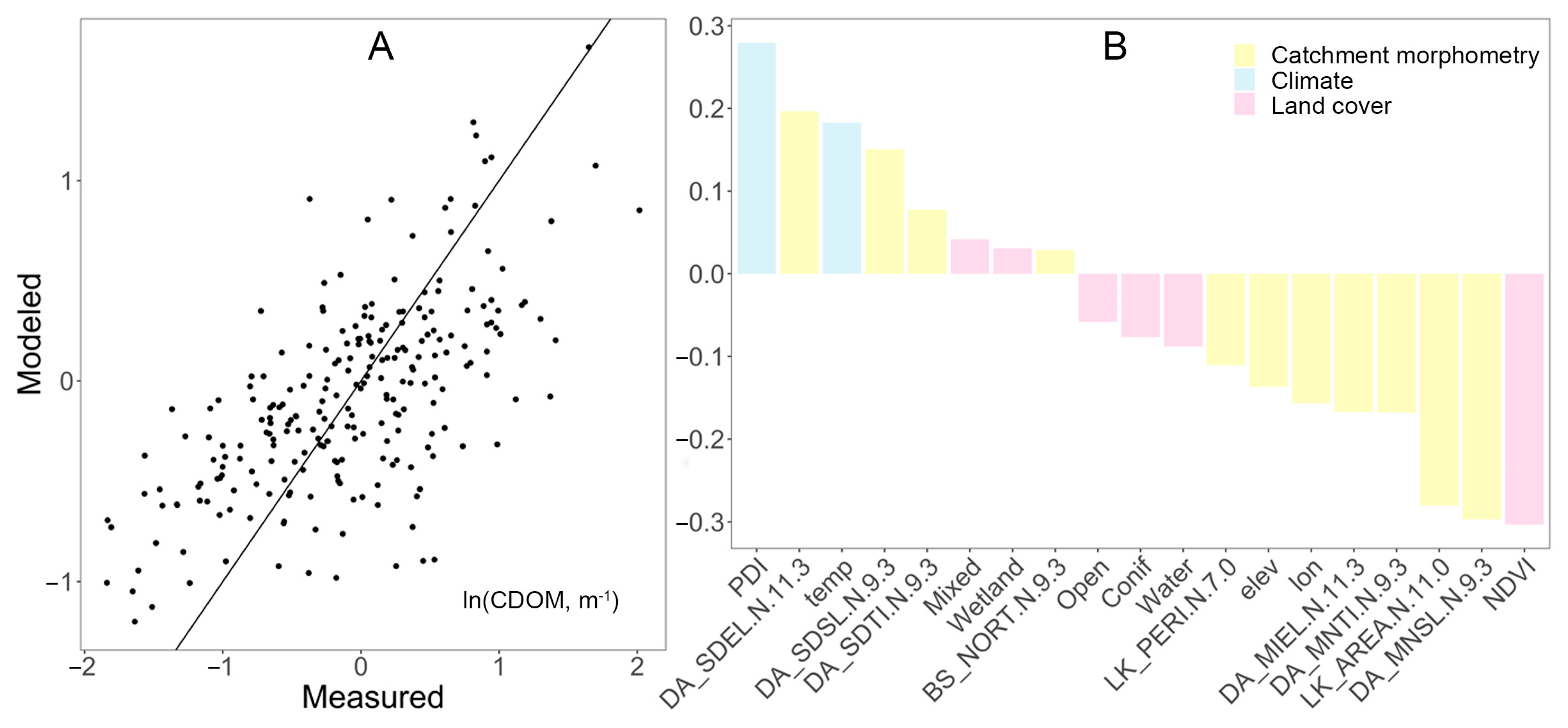
Figure 4.
(A) Performance and (B) variables of importance in a PLS model for natural logarithm of CDOM (m−1) during the wet year of 2016. The model explained 60% of the variance in CDOM, using 76% of the variance in the predictor variables (Table 1).
Figure 4.
(A) Performance and (B) variables of importance in a PLS model for natural logarithm of CDOM (m−1) during the wet year of 2016. The model explained 60% of the variance in CDOM, using 76% of the variance in the predictor variables (Table 1).

Figure 5.
(A) Performance and (B) variables of importance in a PLS model for ln-transformed CDOM (m−1) regressed from predictor variables in the dry year of 2018. The model explained 43% of the variance in CDOM with using 71% of the data variance of the predictor variables. See explanation of selected variables in Table 1.

Figure 6.
(A) Correlation between ln-transformed CDOM (m−1) and air temperature (°C) in the 2016 wet year (y = 0.150x−0.804; R2 = 0.29; p < 0.0001) and 2018 dry year (y = 0.118x−1.397; R2 = 0.09; p < 0.0001). (B) Correlation between ln-transformed CDOM (m−1) and ln-transformed lake area (m2) for the (2018) dry summer (y = −0.117x + 1.495; R² = 0.10). (C) Correlation between ln-transformed CDOM (m−1) and relative catchment cover of coniferous forest area in (2016) wet season (y = 0.664x + 0.576, R2 = 0.19; p < 0.0001).

Figure 7.
(A,B,D,E) The spatial distribution of the strength of the coefficients (temperature and SDTI) and the significance of the spatial points are shown for the respective variables in the wet year 2016. (C,F) The spatial distribution of the strength of the coefficients lake area and the significance of the spatial points are shown for the dry year 2018.


Table 1.
Variables selected by partial least-squares regression analysis (PLSR). See Peters et al. [30] for detailed information about the morphometry variables on the first 13 rows in the table.
Table 1.
Variables selected by partial least-squares regression analysis (PLSR). See Peters et al. [30] for detailed information about the morphometry variables on the first 13 rows in the table.
| Variable ID | Description | Unit |
|---|---|---|
| BS_WIDT.N.6.0 | Basin width | m |
| DA_SDEL.N.11.3 | Drainage area std. dev. elevation | m.a.s.l. |
| DA_MNTI.N.9.3 | Drainage area mean topographic index | unitless |
| DA_SDTI.N.9.3 | Drainage area std. dev. topographic index | unitless |
| BS_CHLM.N.8.3 | Basic Chorley’s lemniscate | unitless |
| BS_SCEL.N.8.3 | Basin Schumm’s elongation | unitless |
| BS_HFF1.N.8.3 | Basin Horton’s form factor 1 | unitless |
| BS_NORT.N.9.3 | Basin orientation northness | unitless |
| DA_SDSL.N.9.3 | Drainage area mean slope | degrees |
| LK_PERI.N.7.0 | Lake perimeter | m |
| LK_AREA.N.11.0 | Lake area * | m2 |
| DA_MIEL.N.9.3 | Drainage area minimum elevation | m.a.s.l. |
| DA_MNSL.N.9.3 | Drainage area mean slope | degrees |
| temp | Air temperature * | °C |
| PDI | Palmer drought index | unitless |
| lon | Longitude | decimal degrees |
| lat | Latitude | decimal degrees |
| elev | Elevation | m.a.s.l. |
| Herba | Herbaceous vegetation and shrubs | % coverage |
| Wetland | Wetland | % coverage |
| Broad | Broad leaf forest | % coverage |
| Water | Open water | % coverage |
| Mixed | Mixed forests | % coverage |
| Open | Open area | % coverage |
| Conif | Coniferous forest | % coverage |
| NDVI | Normalized difference vegetation index | unitless |
* ln-transformed variable.
Table 2.
Wet (2016) and dry (2018) spatial model for temperature, lake area, and SDTI.
| Year | Model Variables | R2 | AIC | BIC |
|---|---|---|---|---|
| 2016 | Temperature, Lake Area, SDTI | 0.67 | 51.72 | 97.13 |
| 2018 | Lake Area, Wetlands | 0.54 | 427.35 | 462.16 |
Disclaimer/Publisher’s Note: The statements, opinions and data contained in all publications are solely those of the individual author(s) and contributor(s) and not of MDPI and/or the editor(s). MDPI and/or the editor(s) disclaim responsibility for any injury to people or property resulting from any ideas, methods, instructions or products referred to in the content. |
© 2024 by the authors. Licensee MDPI, Basel, Switzerland. This article is an open access article distributed under the terms and conditions of the Creative Commons Attribution (CC BY) license (https://creativecommons.org/licenses/by/4.0/).
Share and Cite
MDPI and ACS Style
Al-Kharusi, E.S.; Hensgens, G.; Abdi, A.M.; Kutser, T.; Karlsson, J.; Tenenbaum, D.E.; Berggren, M. Drought Offsets the Controls on Colored Dissolved Organic Matter in Lakes. Remote Sens. 2024, 16, 1345. https://doi.org/10.3390/rs16081345
AMA Style
Al-Kharusi ES, Hensgens G, Abdi AM, Kutser T, Karlsson J, Tenenbaum DE, Berggren M. Drought Offsets the Controls on Colored Dissolved Organic Matter in Lakes. Remote Sensing. 2024; 16(8):1345. https://doi.org/10.3390/rs16081345
Chicago/Turabian StyleAl-Kharusi, Enass Said., Geert Hensgens, Abdulhakim M. Abdi, Tiit Kutser, Jan Karlsson, David E. Tenenbaum, and Martin Berggren. 2024. "Drought Offsets the Controls on Colored Dissolved Organic Matter in Lakes" Remote Sensing 16, no. 8: 1345. https://doi.org/10.3390/rs16081345
Note that from the first issue of 2016, this journal uses article numbers instead of page numbers. See further details here.