Volume Structure Retrieval Using Drone-Based SAR Interferometry with Wide Fractional Bandwidth

Abstract

Synthetic aperture radar (SAR) interferometry (InSAR) is a well-established remote sensing technique capable of providing accurate topographic information of an area. Multiple scattering occurring at different heights within a single resolution cell, however, cannot be resolved using a single baseline and results in a degradation of the height accuracy. Techniques such as polarimetric InSAR and SAR tomography tackle this problem using additional measurements to obtain the three-dimensional structure of the volume. However, polarimetry-based methods assume orthogonal and deterministic scattering mechanisms and tomography requires numerous observations. This paper presents a novel approach to retrieving the three-dimensional structure of semitransparent media using wide fractional bandwidth InSAR. The frequency dependency of the InSAR coherence is exploited to retrieve the three-dimensional structure, assuming that signals with wide fractional bandwidth are available, as is the case for unmanned aerial vehicles (UAVs) or drones. As the extinction is, in general, frequency-dependent, a third observation may improve the inversion results. Simulations of different scenarios show that the frequency profile can be inverted to obtain information about the three-dimensional scattering structure. The acquired data also enable retrieval of the phase center depth as a function of frequency. This method allows for frequent and accurate monitoring of semitransparent targets, e.g., forests and vegetation, using a swarm of two or three drones.

1. Introduction

Synthetic aperture radar (SAR) interferometry (InSAR) is a well-established technique capable of providing the topographic information of an illuminated scene using two SAR images acquired from vertically or horizontally separated positions [1,2].

Acquiring topographic information using InSAR is adequate for surface scattering with backscatter occurring at a distinct height. In the case of semitransparent media with multiple scattering from different heights in a resolution cell, volumetric decorrelation occurs, adversely affecting the InSAR phase and height measurements [3]. The decorrelation results in a decrease in the magnitude of the InSAR coherence, the complex correlation coefficient between the two SAR images, which can be used for further investigation of the specific area, e.g., to create a forest/nonforest map [4]. Attempts have been made to obtain more information on the vertical structure and use it in digital terrain retrieval [5], measuring above-ground biomass [6,7], forest height retrieval [8,9,10,11,12], radioglaciology [13], identification of hidden objects [14,15], and agricultural monitoring [16]. These applications require additional acquisitions and signal processing.

Polarimetric InSAR (PolInSAR) is a method well known for its effectiveness in forest height retrieval, assuming orthogonal scattering mechanisms from different heights depending on the polarization [17,18,19]. Cloude and Papathanassiou demonstrated the possibility of separating the scattering mechanisms and the associated heights from the ground and volume in a forest [17]. These methods are effective when the orthogonal scattering assumption is valid and each scattering mechanism occurs at a distinct height.

The vertical structure can be investigated by using multiple measurements at different heights and forming a vertical aperture [20,21,22,23,24]. Reigber and Moreira first demonstrated radar tomography by using airborne SAR [20]. The SAR data obtained from different heights are in a Fourier relationship with the vertical reflectivity of the scene. The vertical information can be obtained by algorithms that exploit this relationship, such as beamforming [20,25], backprojection [21], and polar format algorithm [24], given that enough measurements with precise vertical spacing are available.

Alternatively, InSAR coherences from multiple baselines can be used to identify the vertical scattering information [26,27,28,29,30,31,32]. Treuhaft et al. showed that InSAR coherence can be modeled using the vertical wavenumber according to the scattering profile [31]. Treuhaft et al. attempted to exploit the relationship by acquiring InSAR pairs for different vertical wavenumbers using multiple flights and retrieving the forest density profile from the acquired data [32]. Cloude demonstrated that sophisticated vertical scattering profiles could be obtained using multibaseline PolInSAR data [26]. Tebaldini proposed a general approach to use the covariances of multibaseline PolInSAR data to separate multiple scattering mechanisms within a resolution cell [29].

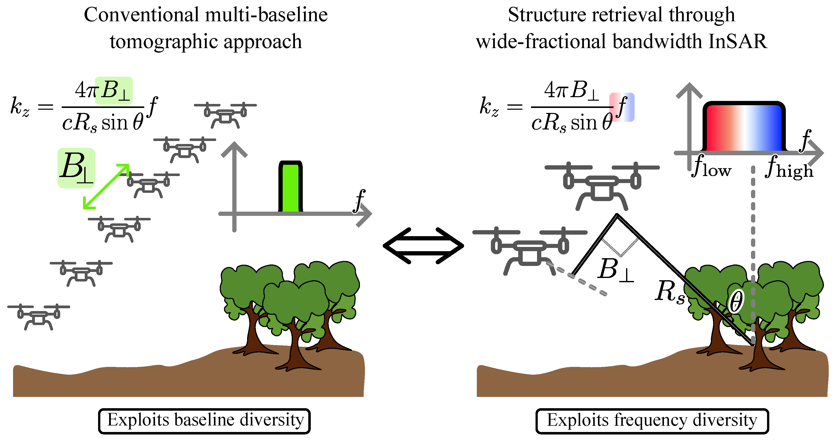
While the tomographic methods use multiple baselines (i.e., a vertical aperture) and do not require the orthogonal scattering assumption, they require tens of measurements in the vertical direction to properly investigate the volumetric characteristics. The vertical wavenumber $k_z$ is the height-to-phase conversion factor used to model the coherence in multibaseline approaches and can be written (in the case of repeat-pass measurement) as follows:

$$k_z=\frac{4\pi B_{\perp }}{c{R}_{s}sin\theta }f,$$

(1)

where $B_{\perp }$ is the perpendicular baseline, c is the speed of light, $R_s$ is the slant range to target, $\theta$ is the incidence angle, and f is the frequency [1,2]. A constant frequency f is assumed in conventional radar systems with a narrow fractional bandwidth. Data from multiple vertical tracks are therefore needed to estimate the coherence over a span of vertical wavenumbers as depicted in Figure 1 (left). The simultaneous acquisition of all SAR images requires a fleet of planes with airborne sensors or a formation of satellites, i.e., complex and costly systems. SAR images acquired in repeat-pass mode lead instead to temporal decorrelation, which might be severe in spaceborne cases due to the limited revisit times.

Local areas could also be monitored using drones or unmanned aerial vehicles (UAVs), which are easy-to-deploy and low-cost platforms for the investigation of remote scenes and local areas [33,34,35,36,37,38,39]. SAR systems on drones are usually equipped with radars with transmit signals spanning over multiple frequency bands and therefore leading to high resolutions. Burr et al. demonstrated the usage of a radar mounted on a drone platform for high-resolution InSAR measurement, which was capable of generating high-resolution digital elevation models (DEMs) [33].

It is expected that a practical coverage of more than $1$ km² is possible in $30$ min using a drone flying at $120$ m altitude (the maximum allowed by law in Germany). A drone operating at $6$ m/s can travel $10,800$ m in $30$ min. Considering a ground range swath of 100 m, achievable with an antenna beamwidth and look angle of 30° and 43°, respectively, the maximum coverage using a straight path with a long azimuth is over $1$ km². The range coverage can be extended by exploiting the maneuverability of the drones to change directions without changing the orientation. After a sufficient azimuth is covered, the drone can change directions parallel to the ground range and travel so that the antenna footprint does not overlap with the previous track and thereafter perform additional measurements in azimuth. This can be repeated, creating a serpentine-like track, to extend the range swath and still cover more than $1$ km² assuming, e.g., eight separate azimuth tracks of $1250$ m.

While the drone platform provides a practical solution to SAR and InSAR measurements using a single baseline, this is no longer the case for tomography. For a single-pass measurement with multiple receivers, flight control, considering the risk of collision, and hardware synchronization is an issue. Repeat-pass measurements share the drawbacks of the aforementioned airborne and spaceborne tomographic approaches and may require large amounts of power supply for each data acquisition.

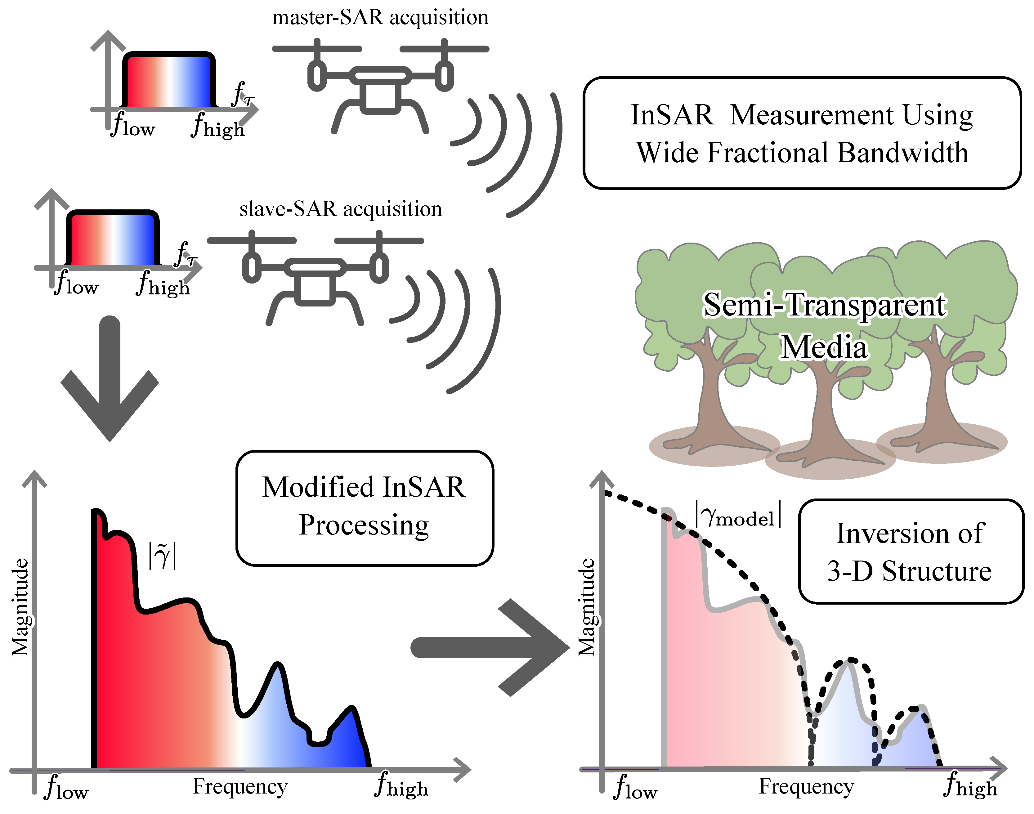
This paper proposes a method to retrieve the volume structure using InSAR data with wide fractional bandwidth. As shown in Figure 1 (right), the use of wide fractional bandwidth signals allows obtaining SAR data with a significant variation in the coherence over frequency. By applying a modified InSAR processing to the pair of SAR data, a coherence trend as a function of the frequency (or of the wavenumber) is obtained [40]. The inversion can then be carried out by comparing different coherence models derived from vertical scattering profiles with the measured coherence trend.

The proposed method requires a very small number of baselines, in practice only one or at most two, to invert the volume structure compared with the conventional tomographic approach, since a single InSAR measurement yields multiple coherence values over a wide range of vertical wavenumbers. Using a single baseline greatly reduces the measurement complexity and implementation costs, broadening the usage of this technique to applications such as frequent forest, ice, and agriculture monitoring. This method has been recently patented [41].

The transmitted frequency assumed in this paper spans over L-, S-, and C-bands to obtain sufficient coherence measurements in the vertical wavenumber. As such, transmit frequencies are currently regulated for airborne and spaceborne platforms, and the proposed method can be combined with drone platforms for the three-dimensional investigation of local and remote areas.

This paper is organized as follows. In Section 2, an overview of the proposed method and its principles is given. In Section 3, the method is explained in more detail, with emphasis on the data processing and inversion steps. In Section 4, simulations are presented, including a description of the simulated data generation, the coherence trend estimation, and the inversion. Conclusions are drawn in Section 5.

2. InSAR Using Wide Fractional Bandwidth Data

2.1. Method Overview

A high-level graphical representation of the proposed method to invert the three-dimensional structure of a semitransparent medium using signals with wide fractional bandwidth is depicted in Figure 2.

As shown in the top left-hand side of Figure 2, the proposed method assumes an InSAR measurement from radars with wide fractional bandwidth, where the ratio between the transmit bandwidth and center frequency is larger than one, e.g., from $0.5$ GHz to $5.5$ GHz.

An interferometric coherence map with high range resolution can be obtained from the available measurements using conventional InSAR processing. A modified InSAR processing is introduced to estimate the coherence as a function of frequency for each range and azimuth pixel through bandpass filtering of the range compressed data in frequency. As a result, coherences over a wide range of vertical wavenumbers are obtained at the cost of a degraded range resolution of the coherence maps. The magnitude of the coherence trend varying with frequency is depicted in the bottom left-hand side of Figure 2.

The inversion of the coherence trend is performed by searching for a coherence model that best fits the estimated coherence values, as shown in the bottom right-hand side of Figure 2. A set of parameters that characterize the coherence model can be used to define the vertical scattering profile, which represents the amount of backscatter within a semitransparent medium.

The inversion is possible due to the one-to-one relationship between a vertical scattering profile and the coherence model. The interferometric coherence governs the statistical characteristics of the interferogram when performing InSAR and is the critical quantity to evaluate the InSAR performance [4]. The coherence is a complex number, with its absolute value varying from 0 to 1 and its phase value contains topographic information. The magnitude of the coherence $\gamma$ decreases for signals backscattered from semitransparent media due to volumetric decorrelation.

In traditional single-baseline, narrowband InSAR for DEM generation, the presence of multiple scatterers occurring at different heights within a single resolution cell manifests itself as a loss of coherence (volumetric decorrelation) that leads to worse performance in terms of height accuracy. In the proposed method, the same coherence loss can be exploited to retrieve information owing to the fact that the volumetric decorrelation is not a result of random noise but of the superposition of many scatterers. It was shown by Treuhaft et al. that the coherence can be modeled as an integral over the vertical coordinate, written as follows:

$$\begin{array}{cc}\hfill \gamma & =exp\left[j{\varphi }_0\left(z_0\right)\right]\frac{{\displaystyle {\int }_0^{h_v}exp\left(j\frac{4\pi B_{\perp }}{c{R}_{s}sin\theta }fz\right)g_v\left(z\right)dz}}{{\displaystyle {\int }_0^{h_v}{g}_v\left(z\right)dz}}\hfill \\ \hfill & =exp\left[j{\varphi }_0\left(z_0\right)\right]\frac{{\displaystyle {\int }_0^{h_v}exp\left(j{k}_{z}z\right)g_v\left(z\right)dz}}{{\displaystyle {\int }_0^{h_v}{g}_v\left(z\right)dz}},\hfill \end{array}$$

(2)

where j is the unit imaginary number, ${\varphi }_0\left(z_0\right)$ is the topographic phase with respect to the ground $z_0$, z is the height from the ground, and $g_v\left(z\right)$ is the vertical scattering profile [31]. The vertical wavenumber $k_z$ is defined in (1). There is therefore a Fourier relationship between the vertical scattering profile $g_v$ and the coherence $\gamma$.

Many SAR systems utilize large bandwidths to achieve high range resolution. Nevertheless, their fractional bandwidth, defined by the ratio between the bandwidth and center frequency, is small. As a result, the change in wavelength is negligible, and the wavelength, given by $f/c$ in (2), is considered constant. Multiple values of coherences over the vertical wavenumber are sampled using multiple baselines in coherence tomography, which requires either a long multitemporal data acquisition or complex SAR systems for single-pass tomographic acquisitions.

In contrast, if a wide fractional bandwidth is available, e.g., from $0.5$ GHz to $5.5$ GHz, the change in vertical wavenumber, and accordingly the expected coherence, is significant. The coherence $\gamma$ can be modeled as a function of varying vertical wavenumber $k_z$ and sampled over a wide range of vertical wavenumbers.

Assuming a uniform backscattering within the volume height $h_v$, the vertical scattering profile can be written as a function of the only parameter $h_v$ as follows:

$$g_v(z;h_v)=\mathrm{rect}\left[\frac{z-h_v/2}{h_v}\right],$$

(3)

where $\mathrm{rect}$ denotes a window function with $\mathrm{rect}\left[x\right]=1$ in $-1/2<x\le 1/2$ and zero elsewhere [42]. The coherence model for (3) can be calculated using (2), which yields

$$\gamma (k_z;h_v,z_0)=exp\left[j\left({\varphi }_0\left(z_0\right)+\frac{h_v{k}_z}{2}\right)\right]\mathrm{sinc}\left[\frac{h_v}{2\pi }{k}_z\right],$$

(4)

where $\mathrm{sinc}$ is defined as $\mathrm{sinc}\left(x\right)=\sin \left(\pi x\right)/\left(\pi x\right)$. The coherence model in (4) can be used for the inversion depicted in Figure 2, assuming that the vertical scattering profile of the semitransparent medium is uniform. The height can also be retrieved by inversion of the coherence magnitude, which does not depend on the topography $z_0$:

$$\left|\gamma (k_z;h_v)\right|=\left|\mathrm{sinc}\left[\frac{h_v}{2\pi }{k}_z\right]\right|.$$

(5)

2.2. Vertical Scattering Models with Constant and Frequency-Dependent Extinction

An example of a coherence model is given in (3), assuming constant backscattering within the volume, which results in a single parameter $h_v$. This model does not foresee an extinction of the signal through the medium. This assumption is not valid for most semitransparent media, such as vegetation.

It was shown by Treuhaft et al. that the backscattered signal from randomly oriented vegetation can be modeled using the extinction coefficient which accounts for the scattering and absorption within the volume [30,31]. This is referred to as the random volume model and is widely used for the investigation of vegetation and ice sheets. The model accounts for the attenuation of the electromagnetic wave through the volume and is expressed using two parameters, $h_v$ and $\sigma$, as follows:

$$g_v(z;h_v,\sigma )=exp\left[\frac{2\sigma }{cos\theta }\right]\mathrm{rect}\left[\frac{z-h_v/2}{h_v}\right],$$

(6)

where $\sigma$ denotes the two-way extinction coefficient.

Using (2) and (6), the coherence model for vertical scattering profiles with extinction can be obtained [28]. The coherence model expressed in vertical wavenumber does not depend on the measurement parameters, e.g., the change in parameters such as baselines does not change the expected coherence value when the vertical wavenumber is constant. Therefore, the measurement parameters can be selected to measure the coherence with respect to a specific region of the coherence model.

The SAR data from a wide fractional bandwidth signal exhibit high variation in wavelength. As a result, the extinction coefficient of the random volume model may change [42,43]. The variation in the extinction coefficient as a function of frequency corresponds, from a physical point of view to a variation in the phase center depth over frequency, which can be directly linked to the phase of the complex coherence for each frequency.

L. A. Bessette and S. Ayasli conducted experiments to measure the coefficients $\alpha$ and $\beta$, which model the attenuation through volume with regards to frequency [43]. Assuming a constant attenuation through media, the relationship between the coefficients and the two-way extinction coefficient $\sigma$ can be expressed as a function of frequency as follows:

$$\sigma \left(f\right)=\frac{\alpha }{30}{\left(\frac{f}{1\mathrm{MHz}}\right)}^{\beta }[\mathrm{dB}/\mathrm{m}].$$

(7)

As a result, the vertical scattering profile is a two-dimensional function of frequency f and height from ground z, expressed using three parameters, $h_v$, $\alpha$, and $\beta$. The expected coherence can be calculated using (2) assuming a constant extinction coefficient over a small extent of frequency.

The inversion results can be ambiguous for the frequency-dependent case if a single baseline is used, i.e., different combinations of parameters might lead to the same coherence profile. This can be partially improved by using an additional platform that provides two additional baselines and therefore three coherence measurements.

2.3. Requirements for Data Acquisition

According to (1), the vertical wavenumber is dependent on the transmitted frequency and geometric parameters. Therefore, the geometric parameters can be selected to measure the coherence trend with regards to a specific region in the vertical wavenumber. For example, to ensure that the region includes the first minimum in (4), the following criteria can be used:

$$\frac{c{R}_{s}sin\theta }{2h_{\max }{f}_{\max }}<B_{\perp }<\frac{c{R}_{s}sin\theta }{2h_{\max }{f}_{\min }},$$

(8)

where $h_{\max }$ denotes the maximum vertical height expected in the area of interest, and $f_{\max }$ and $f_{\min }$ denote the maximum and minimum frequency of the transmitted signal, respectively.

In single-pass acquisitions, the vertical wavenumber is defined as the half of the value defined in (1), e.g., $k_{z,\sin \mathrm{gle}-\mathrm{pass}}=k_z/2$ [44]. In this case, the values of the boundaries in (8) are reduced by half, which can lead to baseline values too small for safe drone operation. The proximity between platforms can be maintained, while abiding the criteria in (8), by introducing a component of the baseline parallel to the radar line of sight.

The modified InSAR processing can be used to measure multiple coherence trends in case of additional SAR measurements. Assuming an additional measurement, two additional baselines are available from the set of SAR data, and therefore, three coherence trends can be estimated. The additional baselines can be selected according to (1) so that additional regions in vertical wavenumbers are obtained. A guideline for choosing the additional baseline could be that the coherence trend obtained from the smaller baseline overlap by half of that from the larger baseline in the vertical wavenumber to observe the frequency-dependent behaviors of coherence. This can be accomplished by acquiring a third datum with a baseline equal to $f_c/f_{\max }·B_{\perp }$.

3. Data Processing and Inversion

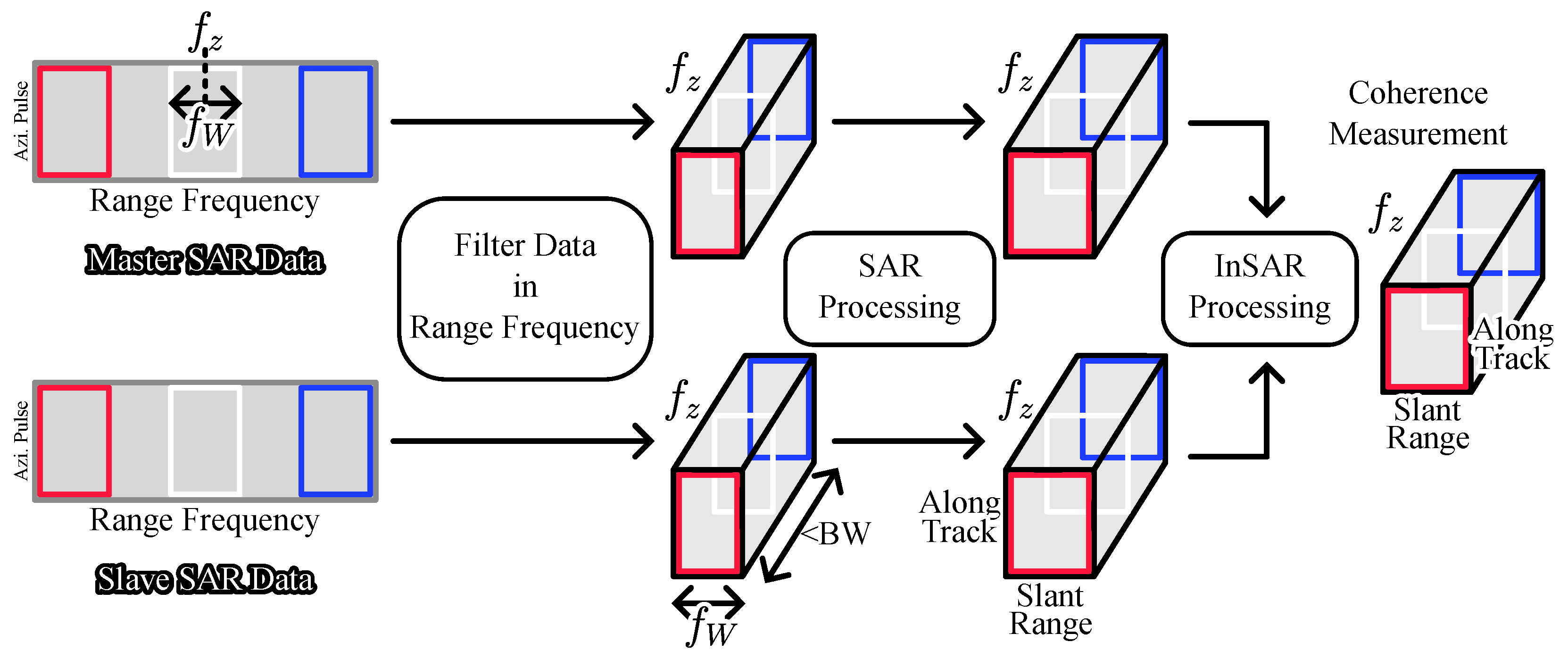
Figure 3 schematically depicts the modified InSAR processing used to estimate the coherence as a function of the frequency or the vertical wavenumber. The pair of SAR data, denoted as master SAR and slave SAR data in Figure 3, is assumed to be range-compressed, Fourier-transformed in fast time, and stored in the form of two-dimensional matrices, where each dimension represents the range frequency and azimuth pulse number, respectively.

In conventional InSAR processing, the range compressed data undergo SAR processing steps to generate a two-dimensional matrix with slant range and azimuth in the spatial domain. In the proposed method, the data are first filtered repeatedly in range frequency and stored in the form of a three-dimensional matrix, where the third dimension represents the center frequency of the filter $f_z$. The passband filters are characterized by a common frequency window width $f_W$ much larger than the change in center frequency, i.e., the filters are highly overlapped, to estimate the continuous change in coherence as a function of the vertical wavenumber.

Azimuth compression is performed on the data [45]. The three-dimensional focused SAR data are represented with two spatial dimensions, slant range and along track, and a frequency axis that defines the frequency windows.

The pair of SAR data are used to perform InSAR processing, which includes image coregistration, ground phase removal, and coherence measurement [1,2]. In this step, the ground phase should be calculated with regard to the center frequency of the window $f_z$. The InSAR coherence is estimated as follows:

$$\tilde{\gamma }=\frac{{\displaystyle \sum _i{s}_1·s_2^{*}}}{{\displaystyle \sqrt{{\displaystyle \sum _i}|s_1{|}^2{\displaystyle \sum _i}{|s_2|}^2}}},$$

(9)

where $\tilde{\gamma }$, $s_1$, and $s_2$ denote the measured coherence, the data from master acquisition, and the data from slave acquisition, respectively. In (9), i is the index of the samples of $s_1$ and $s_2$, i.e., it is assumed that multilooking is performed by spatial averaging over the range and azimuth dimensions.

A sufficiently wide frequency window width $f_W$ is required for the inversion based on the coherence model in (2). The coherence model assumes a constant incidence angle $\theta$ when performing the multilooking for coherence estimation. However, a small frequency window width $f_W$ results in a large range resolution for the same number of looks, and consequentially a large difference in incidence angles, which can be severe in near-field acquisitions such as drone-borne SAR. Contrarily, the span of the frequency axis $f_z$ available for coherence estimation is $BW-f_W$, i.e., a larger frequency window results in a smaller span in vertical wavenumber, where $BW$ is the bandwidth of the transmitted signal.

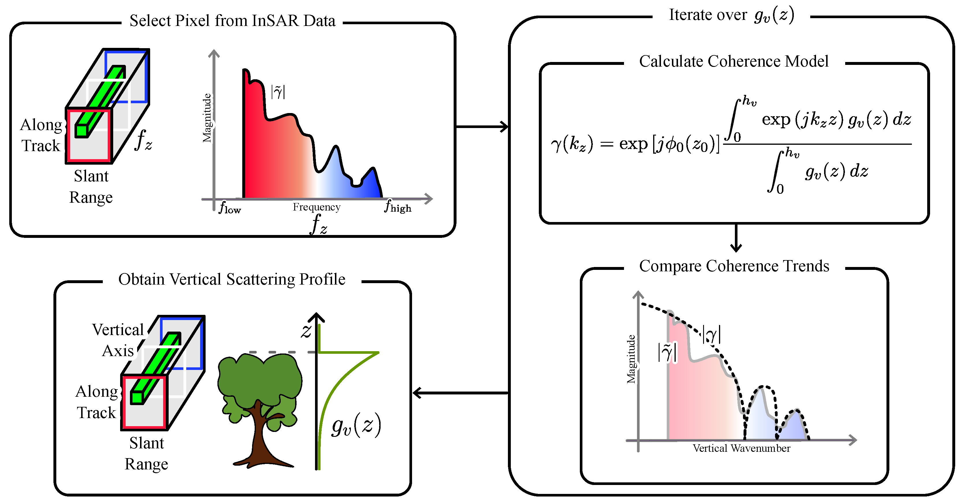
Figure 4 schematically depicts the method used to invert the estimated coherence into the vertical scattering profile. A pixel of interest is selected from the slant range and azimuth axis. Due to the highly overlapped filters used in the modified InSAR processing, a continuous change in coherence with respect to frequency is obtained, referred to as the coherence trend. The frequency axis of the coherence trend $f_z$ can be transformed into the vertical wavenumber using (1) and the known parameters.

The vertical scattering profile is obtained by comparing the coherence trend and the coherence model. The relationship between the coherence model and the vertical scattering profile is given in (2). The comparison is performed to find a coherence model that is the most similar to the measured coherence trend. The minimization of the root means squared (RMS) difference between the coherence model and the coherence trend was used as a criterion to determine the vertical scattering profile.

For the comparison, in the case of uniform backscattering, the complex coherence provided in (4) can be used. However, if the underlying topography is not known, it might be advantageous to use the coherence magnitude provided in (5), because the mutual dependence between the volume height $h_v$ and topography $z_0$ might make the inversion ambiguous in case the backscatter contribution from the bottom part of the volume is limited. In case the coherence magnitude is used, a further improvement could include compensation for its bias and account for the different variances of its estimates for different coherence levels. In case only the coherence magnitude is exploited for the inversion, the phase of the complex coherence can still be utilized to retrieve information about the phase center depth and, under some assumptions, on the penetration depth, as shown in Section 4.4.

Searching through all possible vertical scattering profiles to invert a single pixel is not feasible. Therefore, the vertical scattering profile is modeled using a set of parameters, and a limited number of comparisons are made by varying the parameters. If the vertical scattering profile is analytically expressed as (3), the coherence model can be derived as (4), and the comparison can be performed. In case complex coherence trends are used for the inversion, the topographic height $z_0$ should be considered as a further parameter to be estimated. In particular, the topographic height contributes to the coherence model with a linear phase ${\varphi }_0\left(z_0\right)=k_z{z}_0$. The spectral decorrelation should also be considered when comparing the estimated coherence with the volume decorrelation expected from the model within the inversion [46,47]. The computational complexity can also be reduced using nonlinear parameter estimation methods.

The vertical scattering profile is selected based on the coherence model with the highest similarity. By iterating the process over all pixels of interest, the volume structure is retrieved by the three-dimensional reflectivity data on the along track, slant range, and vertical axis.

4. Numerical Simulations

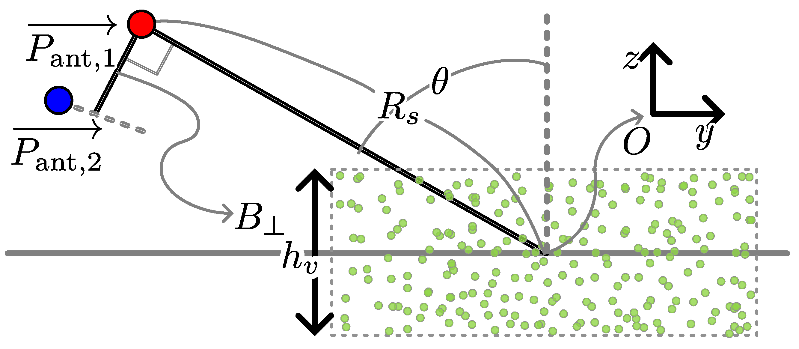
The proposed method was applied to simulated radar data to assess their volumetric inversion capabilities. The simulated radar data were generated assuming a repeat-pass InSAR measurement employing signals with wide fractional bandwidth. The geometry assumed in the simulation is shown in Figure 5, where the positions of the master and slave acquisitions are denoted as $\overrightarrow{P_{\mathrm{ant},1}}$ and $\overrightarrow{P_{\mathrm{ant},2}}$, respectively.

Considering a radar mounted on a drone, the height and slant range of the master acquisition were assumed to be $100$ m and $200$ m, respectively. Accordingly, the incidence angle at the scene center was 60°. The position of the slave acquisition was defined so that the perpendicular baseline was $3$ m.

The backscatter from a semitransparent target was simulated by assuming multiple point targets near the origin. Assuming M point scatterers within the area of interest, the range compressed signals from the master and slave SAR acquisition in the frequency domain $s_1\left(f_{\tau }\right)$ and $s_2\left(f_{\tau }\right)$ were simulated

$$\begin{array}{cc}\hfill s_1\left(f_{\tau }\right)& =\sum _{m=1}^M{A}_{m}exp\left[-j\frac{4\pi }{c}{f}_{\tau }{R}_{m,1}\right]\hfill \\ \hfill s_2\left(f_{\tau }\right)& =\sum _{m=1}^M{A}_{m}exp\left[-j\frac{4\pi }{c}{f}_{\tau }{R}_{m,2}\right],\hfill \end{array}$$

(10)

where $f_{\tau }$ is the range frequency variable, m is the index of each point scatterer, and $A_m$ is the reflectivity of point scatterers. $R_{m,1}$ and $R_{m,2}$ denote the distances measured from each target position $\overrightarrow{P_{\mathrm{tgt},m}}$ to the master and slave acquisitions, respectively. The frequency of the radar signal was defined as a uniformly sampled variable from $0.5$ GHz to $5.5$ GHz.

The azimuth direction is omitted in the signal model and in the processing, assuming identical velocities and SAR images synthesized to the same along-track coordinates. Along-track bins were simulated with an independent set of randomly generated point targets. The reflectivity of point scatterers was defined according to the vertical scattering profile and the vertical coordinate of the target, e.g., $A_m$ was constant when generating simulated data from a volume with a uniform vertical scattering profile.

The coherence is estimated according to the modified InSAR processing described in Section 3. In this section, the frequency window width $f_W$ was $500$ MHz, and the number of bins in the center frequency $f_z$ was 500. The difference between adjacent center frequencies was $9$ MHz. The coherence magnitude was used for the inversion. Using complex coherence leads to very similar results.

4.1. Estimated Coherence Trend for a Uniform Vertical Scattering Profile

In this subsection, simulated radar data were generated assuming a constant volume height and uniform vertical scattering profile. The reflectivity of the target $A_m$ was constant, and the vertical coordinate of the target $z_m$ was randomly selected within the range of $0<z_m\le h_v$.

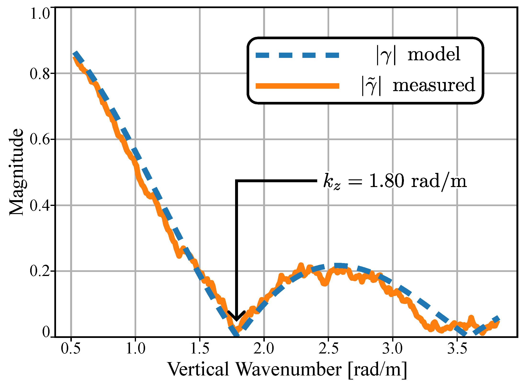
Figure 6 depicts the coherence trend estimated using the modified InSAR processing. The simulated data were generated assuming a volume height $h_v$ of $3.5$ m. The coherence trend, depicted in orange, was estimated using 100 looks (10 looks in azimuth times 10 looks in slant range). The coherence model of uniform vertical scattering in (5) is computed using the simulated volume and height, which are overlapped in the plot using a dashed blue line.

It is observed in Figure 6 that the measured coherence and the model show high correspondence. According to (5), $\left|\gamma \right|=0$ is expected at $k_z=1.80$ rad/m. The low magnitude of the measured coherence trend is evident in the measured coherence trend at the corresponding vertical wavenumber.

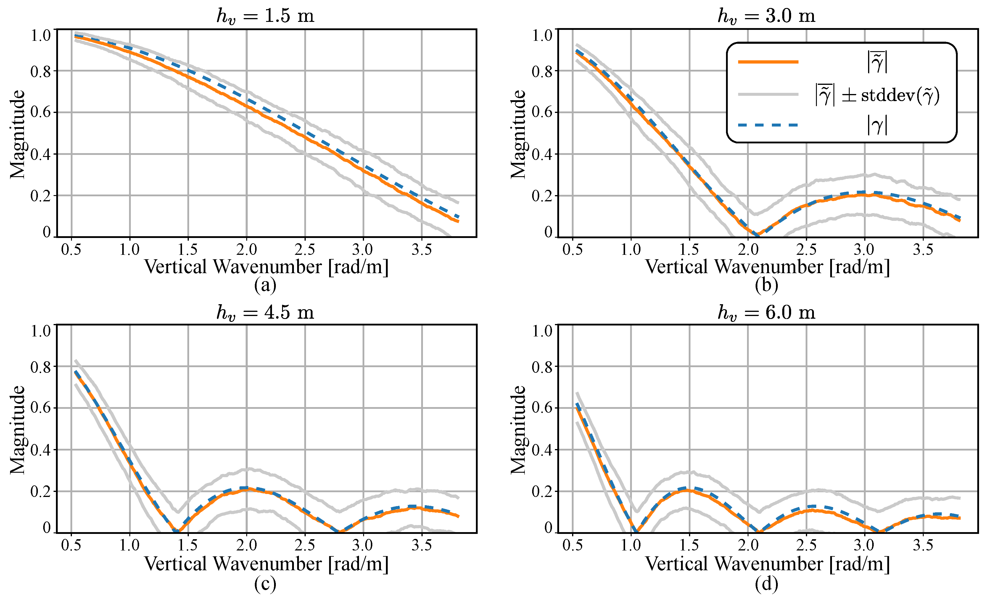
In Figure 7, volume heights of $1.5$ m, $3.0$ m, $4.5$ m, and $6.0$ m are assumed for the cases denoted as (a), (b), (c), and (d), respectively. A total of 100 looks (10 looks in azimuth times 10 looks in slant range) were used to estimate the coherence. For each volume height, 100 coherence trends were estimated from independent simulation targets with common $h_v$. The mean $\left|\overline{\tilde{\gamma }}\right|$ and standard deviation $\mathrm{stddev} \left(\tilde{\gamma }\right)$ were obtained and depicted using orange and gray lines. The coherence models evaluated with corresponding volume heights were overlapped using a dashed blue line. It is observed in Figure 7 that the mean of the estimated coherence converges to the expected values evaluated from the model. The standard deviation increases for larger volume heights and vertical wavenumber. Such variation from the model may adversely impact the inversion performances, and a larger number of looks are required at the cost of decreased slant range and azimuth resolutions.

4.2. Inversion of Random Volume Model with Constant Extinction Coefficient

In this subsection, simulated radar data generated assuming a semitransparent media with extinction are considered. The reflectivity of targets $A_m$ was defined based on the vertical coordinates in accordance with (6).

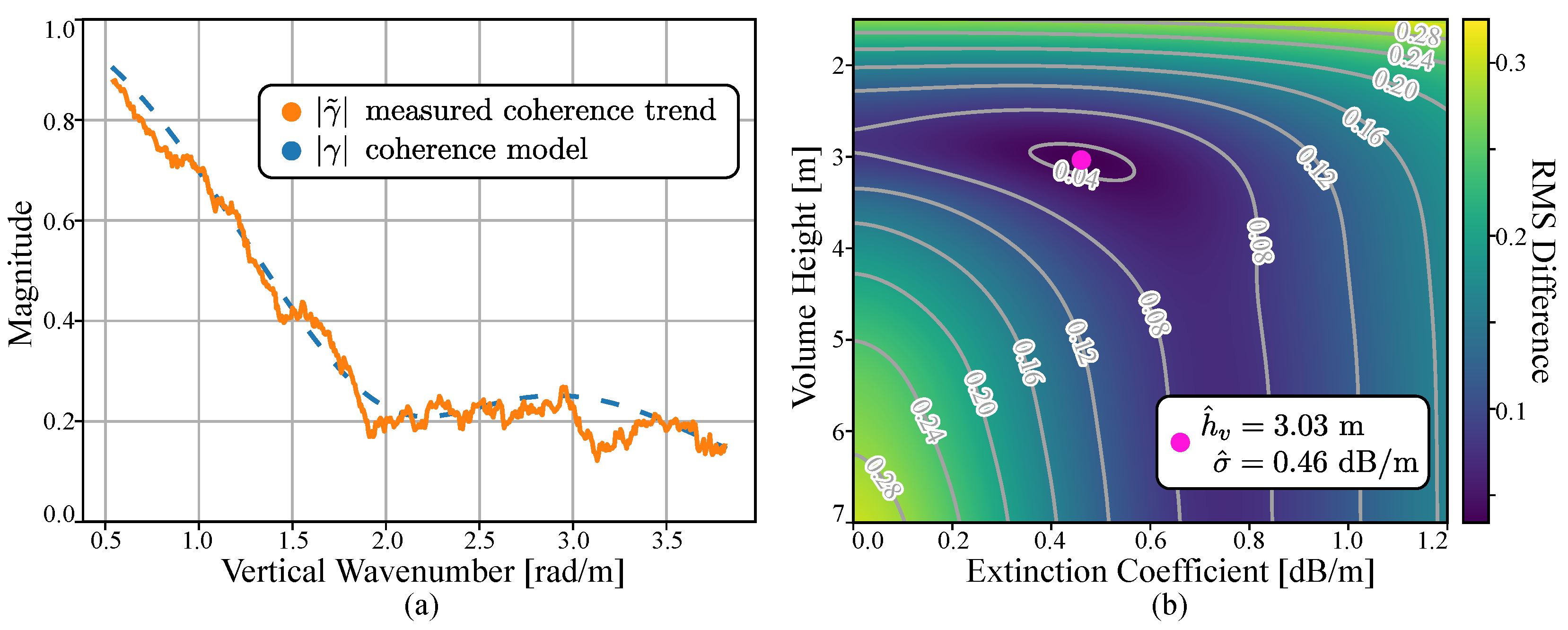
The orange line in Figure 8a shows the coherence trend estimated from simulated data with a volume height $h_v$ of $3$ m and an extinction coefficient $\sigma$ of $0.5$ dB/m. The coherence was measured using 196 looks (14 looks in azimuth times 14 looks in the slant range). The coherence model depicted in blue was evaluated using the corresponding parameters from (2) and (6). The coherence model evaluated with the known values shows great similarity with the estimated coherence trend.

The inversion is performed by finding the coherence model that is most similar to the measured coherence trend. Coherence models were calculated using volume height and extinction coefficients varying from $1.5$ m to $7$ m and from $0$ dB/m (no extinction) to $1.2$ dB/m, respectively. The similarity was evaluated using the RMS difference between the model and the measured coherence trend. Figure 8b shows the RMS difference calculated for all combinations of parameters.

The RMS difference exhibits a smooth surface across the parameter space with a global minimum near the simulated value. The parameters are estimated from the point of lowest difference, which corresponds to the measured volume height and extinction coefficient of $3.03$ m and $0.46$ dB/m.

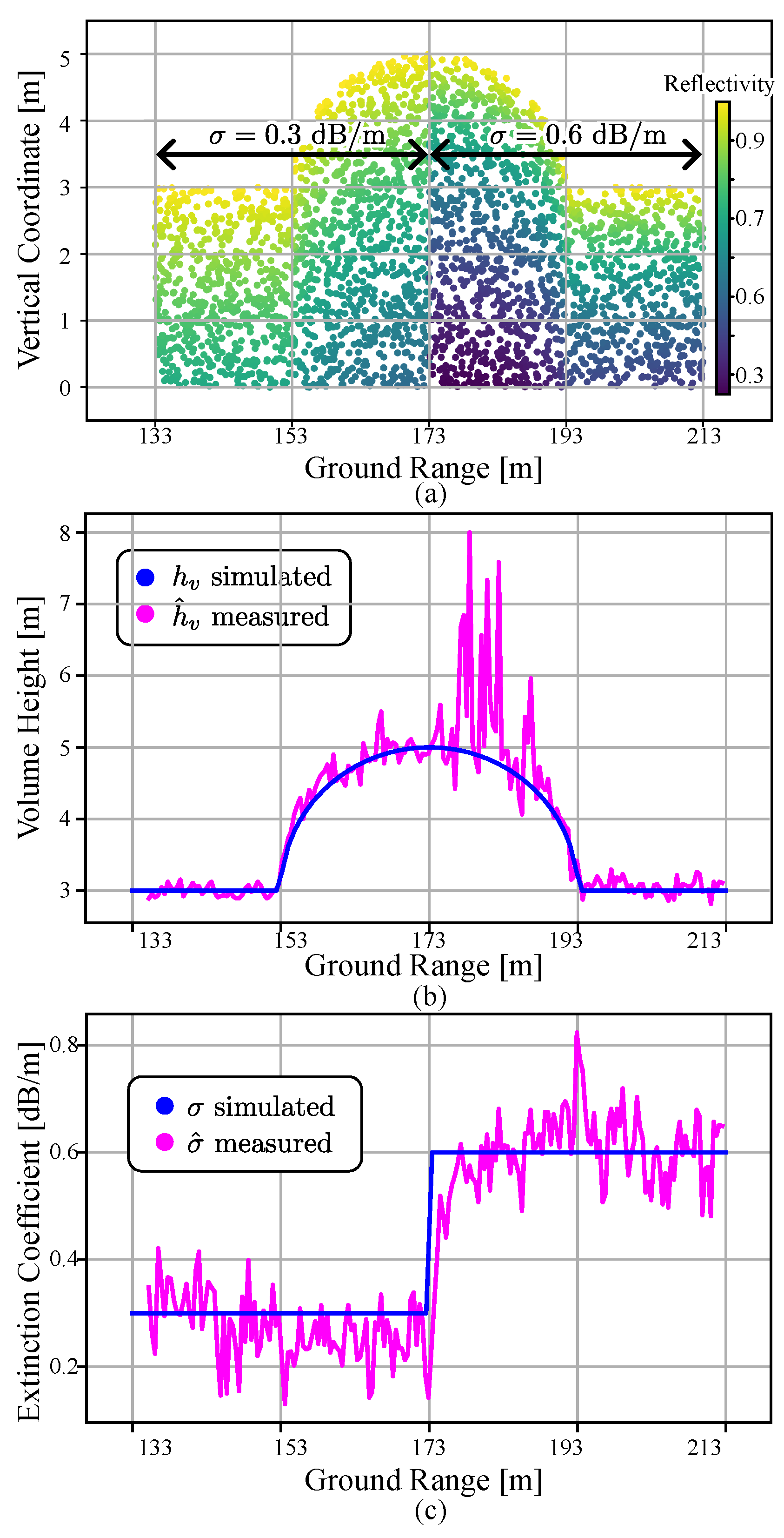
Figure 9a shows an example of simulated targets with varying volume height and extinction coefficient. Point targets are plotted as dots according to their vertical coordinate and ground range. The dots were color-coded according to their reflectivity. The volume height of the scene was a smoothly varying surface with minimum and maximum heights of $3$ m and $5$ m, respectively. The extinction coefficient was $0.3$ dB/m in the near range and $0.6$ dB/m in the far range of the scene.

Figure 9b,c show the volume height and extinction coefficient obtained across the scene with a blue line by iterating the inversion across the slant range. In the parameter estimation stage, the estimated coherence was multiplied by the reciprocal of the expected spectral decorrelation, varying from 0.938 to 0.991, to account only for the volume decorrelation factor [47]. The simulated volume height and extinction coefficients are depicted in orange. The inversion results show that the proposed method is capable of obtaining the vertical scattering parameters for varying volume height and extinction coefficient, especially when the total attenuation through the medium is not significant, i.e., for ground ranges between 133 m and 173 m and between 193 m and 213 m. The estimated parameters can be used to retrieve the volume structure according to the model of the vertical scattering profile.

In Figure 9b, some estimated height values are largely different from the simulated values. The erroneous measurement is evident in the region with large volume height and extinction coefficient. The result is due to the low reflection from the targets with low vertical coordinates, i.e., as the extinction is very high, it is not possible to retrieve information about the lower part of the volume from the scattered signal. This implies that the volume height is not a relevant parameter in these cases. As the extinction coefficient can still be estimated quite accurately, an “effective” volume height, defined as the reciprocal of the extinction coefficient, could be considered as an alternative parameter.

4.3. Vertical Scattering Profiles with Frequency-Dependent Extinction Coefficient

In this subsection, simulated radar data were generated assuming a semitransparent media with frequency-dependent extinction. The reflectivity of the targets $A_m$ was defined based on the vertical coordinates and range frequency to account for the change in extinction coefficient according to (6) and (7). It was assumed that the volume heights $h_v$, $\alpha$, and $\beta$ were $6$ m, $0.31$, and $0.48$, respectively [43].

A third SAR measurement from an additional flight was assumed in this subsection. With the auxiliary acquisition, three SAR datasets were generated, from which three coherence trends from three baselines were obtained. The availability of a second baseline in combination with a wide fractional bandwidth allows retrieving the coherence for a given wavenumber as combinations of different frequencies and baselines and therefore to characterize a frequency-dependent extinction coefficient.

The auxiliary acquisition was assumed to be taken from a position $1$ m away from the master acquisition and $4$ m away from the slave acquisition in the direction perpendicular to the line of sight. As a result, two additional baselines of $1$ m and $4$ m were available.

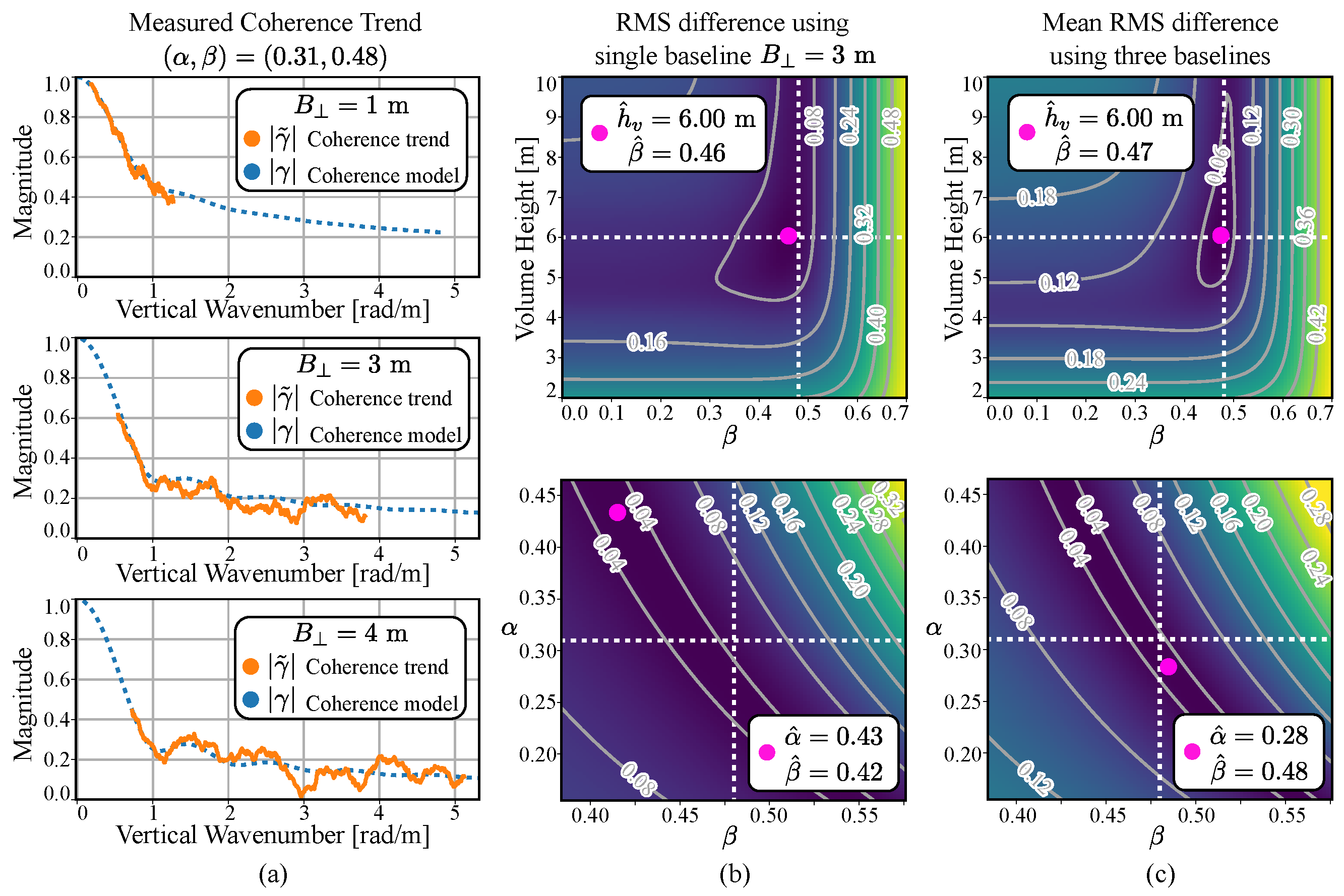
The coherence trends estimated from the three baselines are depicted in Figure 10a. The three trends are labeled using the corresponding baselines, and the measured coherence trend is depicted in orange. The two coherence trends obtained using the auxiliary acquisitions occupy regions with smaller and larger vertical wavenumbers compared with the coherence of the initial baseline $B_{\perp }=3$ m due to the newly acquired baselines of $1$ m and $4$ m, respectively.

Along with the coherence trends, the coherence model is depicted in Figure 10a with blue dotted lines. Due to the frequency-dependent scattering of the volume, the coherence model is no longer common for all acquisition pairs. In the bottom plot of Figure 10a, which corresponds to a baseline $B_{\perp }=4$ m, the differences between the estimated coherence trends and the model are due to the large relative variance in the coherence estimate for low coherence values [1].

The inversion can be carried out by evaluating the similarity using multiple combinations of three parameters $\left(h_v,\alpha ,\beta \right)$. The inversion result is $\left(\widehat{h_v},\widehat{\alpha },\widehat{\beta }\right)=(6.18\mathrm{m},0.46,0.40)$, when the coherence from the single baseline $B_{\perp }=3$ m is used.

Alternatively, the inversion can be performed by incorporating the additional coherence estimates. A simple scheme to use all three coherence trends is to minimize the mean RMS difference using the three coherence trends, which results in $\left(\widehat{h_v},\widehat{\alpha },\widehat{\beta }\right)=(6.00\mathrm{m},0.28,0.48)$. Comparing the obtained results with the true values of $\left(h_v,\alpha ,\beta \right)=(6.00\mathrm{m},0.31,0.48)$, it is apparent that the use of an auxiliary measurement significantly improves the parameter estimation.

Figure 10b depicts the RMS difference calculated from the estimated coherence trends and the model for $B_{\perp }=3$ m. The top figure depicts the RMS difference in a color-coded map for multiple values of volume height $h_v$ and $\beta$ for $\alpha =0.31$. While the map exhibits a smooth surface with minimum values near the simulated ones, the gradient near the simulated values is low, especially with regard to the change in $h_v$.

Figure 10c depicts the similarity measured using the three coherence trends. The similarity was calculated by taking the mean value of the RMS differences measured from the individual coherence trends. The top figure depicts the mean RMS difference for multiple values of volume height $h_v$ and $\beta$. Compared with the top figure in Figure 10c, the map exhibits a high gradient in the values near the simulated parameter. Such a feature is vital for a robust inversion in real scenarios where additional noise contributions are inevitable.

The bottom figures in Figure 10b,c depict similarities in color-coded maps for different values of $\alpha$ and $\beta$ for $h_v=6$ m. The global minimum of the similarity is found at $\left(\widehat{\alpha },\widehat{\beta }\right)=(0.43,0.42)$ when using a single baseline. The estimation using three baselines in Figure 10c bottom exhibits superior results of $\left(\widehat{\alpha },\widehat{\beta }\right)=(0.28,0.48)$ found near the true values depicted in the white dotted lines. However, it is also evident in Figure 10c that multiple pairs of $\left(\alpha ,\beta \right)$ exhibit similar mean RMS differences compared with those calculated from the true values. Such features may be disadvantageous in real scenarios and may require additional information regarding the illuminated scene.

4.4. Retrieval of the Penetration Depths from the Phase of the Complex Coherence

This subsection illustrates how the phase of the complex coherence as a function of frequency can be used for the characterization of the frequency-dependent scattering behavior of the volume. If the topography is known, the topographic phase term in (2) can be removed, and the residual phase can be converted to a phase center depth or elevation bias. The latter is closely related to the penetration depth. According to Dall, the penetration depth $d=-cos\theta /2\sigma$ is dependent on the extinction coefficient for a small relative penetration depth, i.e., $k_z·d\ll 1$ [3].

Two types of volumes with distinct characteristics were modeled using the same point scatterer positions $\overrightarrow{P_{\mathrm{tgt},m}}$ and different reflectivities $A_m$. The first type was modeled assuming an extinction coefficient varying with frequency as in Section IV-C, where the coefficients $\alpha$ and $\beta$ were 0.31 and 0.48, respectively. The second type was modeled assuming a constant extinction coefficient, as in Section 4.2. The extinction coefficient in this case was $0.482$ dB/m, which corresponds to the median extinction coefficient of the first type.

The vertical components of the point scatterer positions were randomly selected within the range $-h_v<z_m\le 0$. A sufficiently large volume height $h_v$ of $20$ m was selected to model both volumes as an infinitely deep volume, which yields a penetration depth independent of volume height. The perpendicular baseline was assumed to be $0.15$ m, which satisfies the small relative penetration depth assumption.

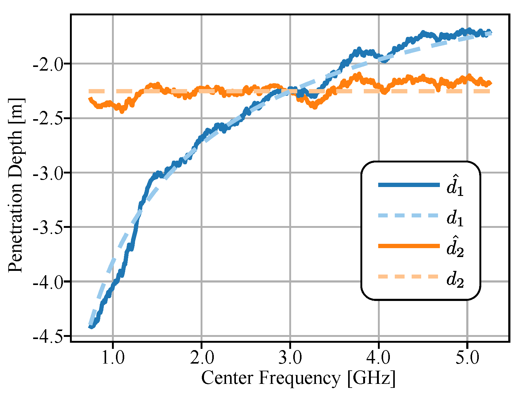
The solid lines in Figure 11 depict the penetration depth calculated with coherence measured from 400 looks (20 looks in azimuth times 20 looks in the slant range). The penetration depth $\widehat{d}=\angle \widehat{\gamma }/k_z$ is calculated by dividing the phase of the coherence by the vertical wavenumber. In the figure, the penetration depths of the first and the second types of volumes are depicted in blue and orange, respectively.

In the case of the constant extinction coefficient, the expected penetration depth $d_2$ is constant and depicted as an orange dashed line. The measured penetration depth of the second type of volume $\widehat{d_2}$ agrees with the expected result. In contrast, the expected penetration depth $d_1$ varies with frequency in the case of a frequency-dependent extinction coefficient, which is depicted as a blue dashed line. The measured penetration of the first type of volume $\widehat{d_1}$ is in good agreement with the expected values. Therefore, one can assess the type of volume scattering by exploiting the relationship between the penetration depth and frequency given that the calibration of the topographic phase is available. Moreover, when the calibration is not available, the nonlinear change in penetration depth or coherence phase can aid in inverting the volumetric scattering parameters of the medium.

5. Discussion

In this paper, a novel method to invert the three-dimensional structure using InSAR data with wide fractional bandwidth is presented. The use of signals with wide fractional bandwidth allows estimating the coherence over a wide range of vertical wavenumbers using a single or a small number of baselines. The proposed method incorporates a modified InSAR processing to estimate the InSAR coherence with regard to a varying wavenumber. The measured coherence is inverted to the vertical scattering profile, and the three-dimensional structure is retrieved.

The proposed method was applied to simulated data assuming volumetric scattering. The coherence was measured using the modified InSAR processing and was compared with coherence models. The performance of the method was verified by inverting the measured coherence to vertical scattering profiles.

To test the proposed method in realistic scenarios, simulated data were generated assuming a semitransparent medium, with scattering dependent on frequency. An additional SAR measurement was considered in this case to aid the inversion performances. The results show that the proposed method is capable of characterizing the volumetric properties in the case of vertical scattering profiles with frequency-dependent extinction coefficient. Finally, a relation between the phase of the complex coherence and the penetration depth as a function of frequency was discussed.

In this paper, RMS was used as the matching criterion in the inversion step. Different matching techniques can be investigated in the future, e.g., considering the statistical characteristics of the expected decorrelation.

This method can further be investigated by using simulated data generated with more general models. Full-wave simulations considering the interaction between elements, e.g., branches of a tree, within the volume can be employed to investigate the inversion performance. Radar data can be simulated based on typical models of the vertical scattering profile, such as the random-volume-over-ground or the multilayer volume, to assess the inversion and even estimate additional parameters, such as the ratio of the backscatter from the ground compared with that from the volume.

A fundamental step to prove the effectiveness of this technique is the demonstration of the proposed method using radar systems mounted on drones. Extensive experiments should be performed over scenes with different volume heights and internal structures. In particular, the acquisition of multibaseline wideband data will enable not only an assessment of the inversion results of the proposed technique but also an understanding of its advantages and drawbacks with respect to traditional narrowband tomography.