Variability Assessment of Global Extreme Coastal Sea Levels Using Altimetry Data

Abstract

This study assesses the variability of coastal extreme sea levels globally by utilizing nearly three decades of along-track, multi-mission satellite altimetry data. An altimetry-based global coastal database of the non-tidal residual sea level component has been produced. The climate variability of extremes is modeled through a parametric, non-stationary statistical model. This model captures intra-annual, inter-annual and long-term variations in non-tidal residual return levels. Comparisons with tide gauge data demonstrate the ability of altimetry data to capture the variability of coastal extreme sea levels. Our findings reveal a greater complexity in the monthly variability patterns of non-tidal residual extremes in tropical latitudes, often exhibiting multiple storm periods, contrasting with coasts in extratropical latitudes, which are mostly controlled by a winter–summer pattern. This study also highlights the significant influence of established climate circulation patterns on sea level extremes. The positive phase of the Arctic Oscillation pattern leads to increases of over 25% in non-tidal residual return levels in Northwestern Europe with respect to a neutral phase. Furthermore, return levels in the western coast of Central America could be 50% higher during El Niño compared to La Niña. Our results show a robust increasing trend in non-tidal residual return levels along most global coastlines. A comparative analysis shows that variations during the 1995–2020 period were primarily driven by intra-annual variations.

1. Introduction

Extreme sea level events pose a significant threat to coastal regions. Flooding episodes induced by these events cause ocean water to penetrate inland, causing erosion and destruction, ultimately leading to significant material (e.g., damaged facilities and material goods), economic (e.g., disruption of economic activities), natural (e.g., wetland degradation), and human losses [1]. Coastal extreme sea levels (ESLs) primarily occur during stormy conditions, i.e., at the landfall of low-pressure systems on the coast or as they move close to them. These events result in a combination of sea level surges induced by low pressures, surges generated by wind stress over the sea surface (i.e., the storm surge), the setup of wind waves, other ocean surface dynamic sea level disruptions (e.g., sea level anomalies due to marine currents), and the astronomical tide. The contribution of the latter is critical along coasts with macro- and meso-tidal ranges [2], as it may become a major contributor to the magnitude and occurrence of ESLs [3,4,5]. Under stormy conditions, sea-level-induced flooding can also combine with strong winds, heavy rain, and extreme events of other ocean surface dynamics, such as wind waves and currents, significantly enhancing the destructive power of storms and exacerbating the resulting consequences in coastal areas. For example, the ocean flooding generated by Hurricane Katrina in New Orleans in August 2005 resulted in monetary losses of over $40 million and over 1500 deaths [6].

Assessing the coastal impacts due to ESLs and designing and implementing coastal management strategies to counter them require knowledge of the maximum sea level magnitudes that can reach the coast [7]. The Extreme Value Theory (EVT) statistically models the behavior of extreme events by fitting an extreme sample to an extreme value distribution, making it possible to estimate the probability of events of an unusual, extreme magnitude to occur, i.e., return periods [8]. High return period events (e.g., 100-year, 500-year) are estimated to model major flooding episodes and assess related flood risk, leading to the adoption of adequate protection measures [9,10].

A comprehensive understanding of ESLs, however, requires consideration not only of the magnitude of the events, but also of their temporal variability. A deep understanding of ESL variability makes it possible to design protective measures that embrace the evolution of events over time. In this regard, the magnitude of ESLs may change in different intrinsic periods, such as seasons, years, or decades, all combining to modulate their occurrence. The non-stationarity of ESLs has already been demonstrated in previous studies at global [11,12], regional [13,14,15], and local scales [16,17,18] based on tide gauge (TG) records and hindcast products. The climate variability of ESLs can be assessed through approaches based on the EVT or alternative methods. The latter requires the establishment of a criterion to classify water level events as storms. The variability of storm events can be assessed by analyzing, for example, the frequency of occurrence or the correlation with climate teleconnection patterns [19]. Approaches based on the EVT typically address ESL variability by conducting an extreme value analysis using parametric statistical models. These models can, for example, introduce a non-stationary behavior on extremes based on time-varying model parameters [16]. Also, pseudo-nonstationary extreme models, such as those fitting a statistical extreme model to moving windows [20], have been proposed.

The magnitude of ESLs is not constant throughout the year. The most severe events tend to be concentrated during storm periods (i.e., consecutive months), alternating with periods characterized by lower magnitudes. This results in a monthly pattern whose complexity depends on the intrinsic variability of the types of events involved. Identifying months prone to suffering the impact of more significant ESLs is especially crucial where these extreme events may cause severe coastal damage, such as those affected by tropical cyclones, and/or where the differences between the strongest and the weakest events within the year are notable. These coasts are suitable for the application of seasonal protection measures. For example, coasts affected by tropical cyclones, i.e., intense events characterized by strong winds and sharp pressure gradients (i.e., very high sea level surges), may adopt measures to reduce their impact, such as the development of seasonal forecasts [21], the implementation of early alert services [22], and the implementation of evacuation plans for major events [23,24]. Coasts affected by highly seasonal extratropical cyclones, such as the northern coasts of the Iberian Peninsula, can also adopt protection measures that account for the variability within the year, such as scheduling beach regeneration measures outside of storm periods [7].

The interannual variability of ESLs can be linked to the intrinsic modulation of atmospheric–ocean circulation patterns. Depending on the phase and intensity of a certain pattern, there may be greater or lesser probability of ESLs occurring. These relationships can be estimated using climate teleconnection indices. Previous research has shown that the position of the Northern Hemisphere (NH) Atlantic extratropical storm track is closely related to the phase of the North Atlantic Oscillation (NAO) teleconnection pattern [25]. Depending on its phase, storms are expected to make landfall further north or south on western European coasts, which consequently affects the magnitude of ESLs at these locations. Similarly, the positive phase of the Southern Annular Mode (SAM) is linked to the landfall of storms along the south Australian coast, whereas during its negative phase, storms travel poleward, reducing the storm activity in the mentioned area [26]. The ENSO phenomenon also modulates storm surges in southeast Asia by altering tropical cyclones and other forcing factors [27].

Long-term variability should also be considered. Today, the effects of climate change over the ocean surface are assumed to be unavoidable in the coming years [28]. Assessing the impact of climate change on ESLs is challenging due to the number of drivers involved. The mean sea level rise (MSLR) [29,30], along with potential changes in atmospheric drivers of ESLs, such as the frequency, trajectory, and intensity of atmospheric storms, may lead to significant increases in extreme events and, consequently, in the severity of associated impacts [31,32]. Recent studies have addressed the assessment of changes in ESLs due to climate change at the global scale based on an ensemble of numerical sea level projections [33,34] or by only considering MSLR [32,35].

The study of sea levels, and specifically, of extreme events, has traditionally been conducted using TG recorded data [11,36,37,38], as they are still regarded as the most reliable providers of sea level information [39]. However, some limitations restrict their use, such as the influence of land movements [40], heterogeneous time sampling, irregular spatial coverage, and the fact that they provide very localized information. Despite these limitations, TG-recorded data offer valuable information for climate studies, helping to reveal, for instance, MSLR as the primary driver of changes in ESLs [11,41]. Numerical models, leveraging technological advancements, have emerged as an alternative to in situ information for the study of sea levels, enabling EVAs at different spatial scales. For example, the study by Muis et al. (2016) [42] provided global 100-year return level water levels based on global simulations of the hydrodynamic numerical model GTSM. Similarly, 10-year return levels are provided using the GTSM3.0 model [33]. Additionally, Zhang and Sheng (2015) [43] provided 50-year return level total water levels for the northeast Pacific Ocean using the ocean circulation numerical model POM. Numerical models have also been extensively used to model the sea level variations generated by individual events [44]. Nevertheless, numerical simulations have not yet been able to accurately characterize the peak maximum values of ESLs, mainly due to the resolution of atmospheric forcings [42].

Satellite altimetry stands as a new sea level data source that has provided information since the 1990s globally, thus overcoming one of the major limitations of TG data: heterogenous spatial coverage. Furthermore, the current length of this database, approximately 30 years, makes it possible to partly overcome the characteristic irregular spatial and temporal resolution of altimetry data. Altimeters sample along their tracks at a characteristic rate (e.g., Altika samples at 1 Hz), so that each altimeter measurement is characterized by specific coordinates and sampling times. This issue means that satellite products with processing levels below L4 (i.e., non-gridded products) present irregular spatial and time coverage. The combination of long records and continuous accuracy improvements, particularly in coastal areas [45,46], supports the use of altimetry data for validation purposes (Stammer et al., 2014 [47]) and to develop climate studies. The main climate outcome based on altimetry data over the last three decades is the estimation of historical MSLR trends [39,48,49]. Moreover, despite these trends typically being provided for the deep ocean, both at global [50,51] and regional [52,53,54] scales, the increasing accuracy nearshore makes it possible to estimate coastal MSLR trends in coastal areas with notable precision [55,56]. A clear example is the set of virtual altimetry stations developed within the Climate Change Initiative, which provides sea level anomaly (SLA) time series and identifies trends along the global coasts [57,58,59]. Other sea level climatic features have also been studied using this type of data, such as the relation between SLAs and climate teleconnection patterns [60], and the seasonal and mesoscale variability of sea levels [61]. Satellite altimetry data have also been used to analyze the sea level surges induced by specific cyclonic events, such as Hurricane Isaac in in 2012 in the Gulf of Mexico [62]. However, the use of altimetry data for climate variability studies on ESLs on coastal areas remains limited [63].

In this context, this study aims to evaluate the global climate variability of ESLs using satellite altimetry data. Among the different components of ESLs mentioned earlier, this research specifically focuses on the non-tidal residual (NTR) sea level component, which represents sea level oscillations with respect to mean sea levels with a non-tidal origin. Consequently, this study aims to provide global coastal NTR extreme estimates associated with different return periods, and primarily, to assess their climate variability on various time scales.

This manuscript is structured as follows: Section 2 describes the data used to develop the study and presents the methods applied. Section 3 addresses the validation of the altimetry data and summarizes the main results obtained in the study. Finally, the main conclusions presented in Section 4.

2. Materials and Methods

2.1. Sea Level Altimetry Data

In this study, a global SLA dataset provided by the Copernicus Marine Environment Monitoring Service (CMEMS) was used. It includes inter-calibrated, multi-mission along-track altimetry data measured by more than twenty missions from 1992 onward and processed through the DUACS multi-mission processing system [64]. The study focused on a 28-year period from January 1993 to December 2020, which nearly meets the minimum climate period of 30 years recommended by the World Meteorological Organization (WMO) for climate studies. The SLA dataset is computed by subtracting several sea level components, such as tides and the atmospheric sea level components, from the still water levels measured by the altimeters, i.e., by applying the geophysical corrections [65]. Besides the SLA, this dataset provides dynamic atmospheric correction (DAC), which represents sea level variations due to the effects of atmospheric pressure and wind. More information on the corrections applied to altimetry measurements can be found in [65]. The product can be access at https://data.marine.copernicus.eu/product/SEALEVEL_GLO_PHY_L3_MY_008_062/description (last accessed on 1 March 2024).

2.2. In Situ Data for Validation

The ability of altimetry data to capture the climate variability of NTR extremes was assessed using data recorded from a global set of 400 TGs. Hourly still water level TG records from January 1993 to December 2018 were downloaded from the legacy data portal at the University of Hawaii Sea Level Data Center (UHSLC) webpage (http://uhslc.soest.hawaii.edu/data, last accessed on 1 June 2022).

At each station, a tidal analysis was performed using the U-tide tool [66] based on a harmonic fit. The analysis was conducted over a moving two-year time window, with a central one-year effective period and two half-year overlapping periods at both ends of the window. Years with less than 60% of hourly data were excluded (further details on the harmonic analysis procedure can be found in the Supplementary Material). Thus, the NTR sea level signal measured by the TGs (hereinafter NTR_TG) was computed by subtracting the resulting astronomical tide from the still water level time series.

2.3. Climate Teleconnection Indices Data

Three teleconnection indices were considered to assess the interannual variability of NTR extremes: the Arctic Oscillation index (AO), the Multivariate ENSO Index (MEI), and the Dipole Mode index (DMI). Other teleconnection indices, such as the North Atlantic Oscillation (NAO), the Southern Annular Mode (SAM), and the Niño34, were also analyzed. The AO, MEI, and DMI indices were selected due to their stronger correlations with NTR extremes among the explored indices. These three indices are related to the atmospheric circulation of different ocean regions. AO is related to the atmospheric circulation at NH extratropical latitudes, while the ENSO climate pattern, through the MEI index, reflects the interannual climate variability mainly at Pacific tropical latitudes and West Atlantic tropical latitudes. The Indian Ocean Dipole (IOD) climate pattern, through the DMI index, relates to the atmospheric circulation at Indian Ocean tropical latitudes.

Monthly values for AO, MEI and DMI indices were downloaded from the NOAA Physical Sciences Laboratory webpage (https://psl.noaa.gov/gcos_wgsp/Timeseries/, last accessed on 1 April 2022).

2.4. Statistical Extreme Model

Based on the EVT and the non-continuous hourly satellite data sample used in this study, the block maxima approach was selected to model the behavior of NTR extremes through a generalized extreme value distribution (GEVD; Equations (1) and (2)). Unlike the standard approach based on annual maxima as block maxima, we used monthly maxima values as input instead. Monthly maxima, which have been successfully applied in ESL studies [11,16], and the defined coastal units (Figure 1) to select the altimetry data, provided enough data density. Furthermore, the selected maxima provided information on monthly variations within a year.

We included parametric time-dependent terms in the model to introduce the non-stationary behavior of the NTR climate variable. In particular, time-dependent terms to analyze climate variations in ESLs were incorporated in the GEVD location parameter µ(t), where t represents the time. The statistical extreme model considered climate variations at three different time scales: intra-annual, inter-annual, and long-term trends.

A return period is the average time between events of a certain magnitude. Consistently, a return level is the statistical value of a variable associated with a certain return period. The estimation of time-dependent return levels $z_R\left(t, \theta \right)$ at time t (in years), where $\theta$ represents the GEVD model parameters, associated with the return period R (in years), can be done as:

$$z_{tR}=z_R\left(t, \theta \right)=z_R\left(\mu \left(t\right), \sigma ,\xi \right)=\left\{\begin{array}{c}\mu \left(t\right)-\frac{\sigma }{\xi }\left[1-{\left\{-log\left(1-\frac{1}{R}\right)\right\}}^{-\xi }\right] \xi \ne 0\\ \mu \left(t\right)-\sigma log\left\{-log\left(1-\frac{1}{R}\right)\right\} \xi =0\end{array}\right.$$

(1)

where µ(t) is the time-dependent location parameter, $\sigma$ is the scale parameter, and $\xi$ is the shape parameter.

The estimation of integrated NTR return levels ($\overline{z_R}$) associated with a return period (R) for a specific yearly time window [t_i, t_i + T] can be done as [11]:

$$1-\frac{1}{R}=\left\{\begin{array}{c}exp\left\{-{\int }_{t_i}^{t_i+T}{\left[1+\xi \left(\frac{\overline{z_R}-\mu \left(t\right)}{\sigma }\right)\right]}^{-\frac{1}{\xi }}dt\right\} \xi \ne 0\\ exp\left\{-{\int }_{t_i}^{t_i+T}exp\left[\frac{\mu \left(t\right)-\overline{z_R}}{\sigma }\right]dt\right\} \xi =0\end{array}\right.$$

(2)

where T is the time increment in yearly units.

The intra-annual variability was modeled by combining sinusoidal functions with periods of one year and half-year, as:

$${\mu }_s\left(t\right)=\sum _{i=1}^2{\beta }_{2i-1}\cos 2^i\pi t+{\beta }_{2i}\sin 2^i\pi t$$

(3)

where ${\mu }_s\left(t\right)$ is the time-dependent GEVD location parameter related to the intra-annual variability, t is the time, and ${\beta }_i$ are the fitting parameters related to the sinusoidal functions.

The long-term variability (also referred to as long-term trend) was incorporated into the model through an exponential function. The exponential relationship converges to a straight line for values close to 0 of the exponential parameter (${\beta }_{LT}$) and allows the introduction of acceleration for higher values, as:

$${\mu }_{LT}\left(t\right)={\beta }_{0}exp\left({\beta }_{LT}t\right)$$

(4)

where ${\mu }_{LT}\left(t\right)$ is the time-dependent GEVD location parameter related to the long-term variability, t is the time, and ${\beta }_{LT}$ and ${\beta }_0$ are the fitting parameters related to the exponential function.

The inter-annual variability was explored by analyzing significant relationships between NTR monthly maxima and well-known climate circulation patterns. Monthly values of representative teleconnection indices were introduced as a covariate, $CI\left(t\right)$, as:

$${\mu }_{CI}\left(t\right)={\beta }_{CI}CI\left(t\right)$$

(5)

where ${\mu }_{CI}\left(t\right)$ is the time-dependent GEVD location parameter related to the inter-annual variability, t is the time, and ${\beta }_{CI}$ is the fitting parameter related to the covariate term.

Considering all the climate variability scales, the location parameter can be expressed as:

$$\mu \left(t\right)={\mu }_s\left(t\right)+{\mu }_{LT}\left(t\right)+{\mu }_{CI}\left(t\right)$$

(6)

The estimation of the final time-varying location parameter for each location followed an orderly and efficient optimization process. Different combinations of the parametric terms considered led to different µ(t). The optimal parameter was selected based on the maximum likelihood ratio test and the principle of parsimony, namely, minimizing the number of degrees of freedom to avoid over-parameterization of the model [8].

At the initial stage, µ(t) only considered the intra-annual variability. To find the simplest model, we applied a forward algorithm starting from a stationary model (model M₀). Various combinations of sine functions were explored until the optimal one was reached (model M₁):

$${\mu }_{M_1}\left(t\right)={\mu }_s\left(t\right)$$

(7)

where ${\mu }_{M_1}\left(t\right)$ is the time-dependent location parameter related to model M₁.

Next, we incorporated the long-term trend to define model M₂:

$${\mu }_{M_2}\left(t\right)={\mu }_s\left(t\right)+{\mu }_{LT}\left(t\right)$$

(8)

where ${\mu }_{M_2}\left(t\right)$ is the time-dependent location parameter related to model M₂.

Finally, based on M₂, we employed the same process to define model M₃, this time introducing the inter-annual variability parametric term through each analyzed climate index independently. Therefore, M₃ encompassed three different time scales in modeling the climate variability of NTR extremes. The extreme model introduced the influence of climate teleconnection patterns individually, which translated into a different M₃ model for each climate pattern analyzed.

$${\mu }_{M_3}\left(t\right)={\mu }_s\left(t\right)+{\mu }_{LT}\left(t\right)+{\mu }_{CI}\left(t\right)$$

(9)

where ${\mu }_{M_3}\left(t\right)$ is the time-dependent location parameter related to model M₃.

An example of the evolution of $z_{tR}$ considering models M₁, M₂ and M₃ is shown in Figure S2.

2.5. Non-Tidal Residual Coastal Extreme Sample

As stated earlier, this study aims to assess the climate variability of extreme events of the NTR component of sea level. Accordingly, a NTR dataset computed from altimetry data (henceforth NTR_SAT) was required. We used the approach followed by previous studies to compute NTR data from altimetry measurements [63,67,68,69,70], which is schematized in Figure 2. The calculation of the NTR_SAT dataset was done by undoing the DAC, in other words, by re-adding the DAC product to the SLA. The resulting NTR_SAT ($SLA+DAC$) dataset was an along-track product with irregular time and spatial sampling that covered the global ocean. Note that the NTR_SAT accuracy was inevitably affected by the precision of the still active corrections [71].

To assess the global variability of coastal NTR extreme events, we defined 474 coastal units with an approximate length of 500 km and width of 100 km, covering the global coastlines (Figure 1). The size of the coastal units was set to provide sufficient data for the EVA and to correctly capture the climate variability of NTR extreme events. NTR_SAT data were selected within each coastal unit along the global coastlines. Next, monthly maxima were selected at each coastal unit to be used in the following EVA. In order to avoid spurious monthly data, months with fewer than 10 measurements after hourly re-sampling were not considered.

2.6. Extreme Variability Assessment

Several metrics to represent the climate variability of extremes at different time scales were calculated.

2.6.1. Intra-Annual Variability

The extreme variability within the year was quantified by analyzing the intra-annual evolution of NTR return levels following Equation (1). In particular, we analyzed the evolution of the 20-year return level of NTR within a year ($z_{t20}$ in Equation (1)), in other words, we assessed the magnitude variations experienced by events with a return period of 20 years within a year. This was done by considering model M₂ (see Section 2.4) with no trend (Equation (8)), which implied that, despite the statistical model fitted being M₂, the posterior computation of $z_{t20}$ was done assuming that ${\beta }_{LT}=0$. This allowed us to isolate the intra-annual variability and avoided attributing to seasonal variations changes associated with long-term trends. The variability was measured through the coefficient of variation of $z_{t20}$ within a year, designated as CV²⁰, and computed as:

$${CV}^{20}=\frac{{\sigma }^{R20}}{{\overline{x}}^{R20}}$$

(10)

where ${\sigma }^{R20}$ is the standard deviation of $z_{t20}$ and ${\overline{x}}^{R20}$ is the mean of $z_{t20}$ within a year.

Higher (lower) values of ${CV}^{20}$ indicated a stronger (weaker) intra-annual variability in ESLs.

In addition, the most likely months to exhibit stronger extremes were identified. This was achieved by first determining the number of local maxima for $z_{t20}$ within a year, followed by identifying the months in which these maxima occur.

2.6.2. Long-Term Trends

Long-term trends in NTR extremes were assessed through the relative change in $\overline{z_{20}}$ (Equation (2)) between 1995 and 2020, calculated using model M₂, as:

$$∆\overline{z_{20}}=\frac{\overline{z_{20}^{2020}}-\overline{z_{20}^{1995}}}{\overline{z_{20}^{1995}}}$$

(11)

where $\overline{z_{20}^y}$ is the 20-year return level NTR at year y.

2.6.3. Inter-Annual Variability

The relationship between NTR return level variations and teleconnection climate indices was analyzed to assess the inter-annual variability of NTR extremes. In particular, we evaluated the climate anomalies at monthly time resolution in $z_{t20}$ relative to the neutral phase, i.e., the climate index equals zero (CI = 0). The black line of Figure 3 represents an example of $z_{t20}$ incorporating all time-scale variations in the extreme model (i.e., model M₃; see Section 2.4). In particular, the data in Figure 3 belong to a coastal unit located on the north coast of Papua New Guinea, and the climate index introduced in the model was MEI. The black line time series exemplifies the significant differences in $z_{t20}$ between years, with temporal variations higher than 0.3 m. For example, in 2018, a significant increase in 20-year return level NTR corresponded to a very intense La Niña event, whereas in 1997, an important decrease was associated with a very intense El Niño event.

To quantify the anomalies experienced by NTR return levels in response to climate patterns, we estimated time-dependent return levels at a monthly scale over the 28-year period (Equation (1)) using the model M₃ with the trend term deactivated (i.e., ${\beta }_{LT}=0$; blue line in Figure 3). Consistently, to estimate $z_{t20}$ for the neutral phase, we used the same model assuming CI = 0 (red line in Figure 3).

We calculated the percentiles of $z_{t20}$ at a monthly scale for each month, both considering the monthly variability of the climate indices ($P_{ci}^k$), as well as for the neutral phase ($P_n^k$). The comparison between these percentiles allowed us to quantify interannual climate anomalies, as:

$$A^k=\frac{P_{ci}^k-P_n^k}{P_n^k}\times 100$$

(12)

where $A^k$ is the monthly climate anomaly for percentile k.

$A^k$ can be positive and negative. It is positive when return levels increase during a specific phase, and negative for the opposite phase. Our analysis focused on the 10th and 90th percentiles (i.e., $A^{10}$ and $A^{90}$). This analysis was repeated for the three teleconnection patterns analyzed.

2.6.4. Extreme Variability Dominance

To assess the dominance among the different time-scale variability patterns on the changes experienced by NTR return levels over time, the absolute change linked to each variability scale was calculated for the 1995–2020 reference period.

The contribution of the intra-annual variability was quantified as the maximum amplitude of $z_{t20}$ within a year considering model M₃ (Equation (9)) with ${\beta }_{LT}=0$ and $CI=0$.

The contribution of inter-annual variability was quantified by first estimating the maximum amplitude of $z_{t20}$, during the entire period of analysis using model M₃ with ${\beta }_{LT}=0$. Finally, the contribution of intra-annual variability was subtracted to avoid considering this information twice.

The contribution of long-term trend was calculated as the difference between the 20-year return level NTR in 2020 and 1995 considering model M₃ with CI = 0.

3. Results

3.1. Validation of NTR_SAT

3.1.1. Selection of the Validation Extreme Sample

The ability of altimetry data to reproduce the climate variability of NTR_SAT extremes was validated against TG data. From an initial set of 400 TG records, the 123 selected TG records met a number of requirements to ensure fair validation against satellite altimetry data. First, the location of the station was evaluated, rejecting those in highly sheltered and shallow coasts, such as TG stations located inside of atolls or those located upstream of rivers. TG records at these locations are likely to be significantly impacted by local processes that are not correctly captured by altimetry measurements. Additionally, the amount of available data was analyzed, and TG records with less than 75% of hourly data during the validation period (1993–2018) were rejected.

Comparable extreme samples from NTR_TG and NTR_SAT were needed to validate the altimetry data at each TG station. Both datasets represent sea level variations relative to the mean sea level. However, while TG data are measured relative to a defined datum and linked to land-based benchmarks, which implies that land movements affect the measurements, satellite altimetry data are referenced to a global reference frame, and hence, are affected by such movements. Additionally, while TGs measure sea levels at fixed locations with a specific temporal resolution (e.g., 1 h), along-track altimetry data are collected at different locations with a characteristic sampling rate for each platform.

In order to deal with the spatiotemporal inconsistency between both data sources, a method to select a NTR_SAT dataset around each TG station was defined. These samples were selected based on the Pearson correlation [72] (r) between both datasets in the vicinity of TG stations [63]. The correlation between NTR_TG and NTR_SAT was computed at each node of a 0.25-degree regular grid covering a 7.5-degree circular area centered on the station location. Correlations of contemporaneous pairs NTR_TG-NTR_SAT within a 0.25-degree circle centered at each ocean grid node were computed (scheme in Figure S3). Grid nodes with r values lower than 0.5 were rejected. The correlation cut-off was then continuously increased from 0.5 until the mean number of altimetry measurements was approximately 1 measurement per day. To avoid selecting very close-in-time measurements, NTR_SAT was re-sampled to hourly data at each step of the evolution algorithm. The selected 123 TG stations for the validation process are indicated in the map in Figure 1. Finally, the monthly maxima from NTR_TG and NTR_SAT for each station were selected to be used as input in the EVA.

3.1.2. Validation Results

The ability of altimetry data to capture the magnitude of NTR extreme events and their variability over different time scales is addressed in Figure 4. The location of the analyzed TG stations is depicted on the map in Figure 4, with a different marker color/shape for each region. The correlation between monthly maxima from NTR_SAT and NTR_TG at each TG station was calculated, as shown in Figure 4a, along with the root-mean square error (RMSE; more details on the definition of RMSE can be found in [73]). Correlations had a significance level above 0.99 for all stations. The results indicate that over 80% of the stations exhibited r values higher than 0.7, and more than 50% showed r values higher than 0.8, evidencing a strong agreement between both datasets. The stations with the lowest r values, ranging from 0.5 to 0.6, were scattered along the global coastlines and represented less than 5% of the total TGs, not reflecting any discernible spatial pattern and likely due to local processes that were not fully captured by altimetry data. In general, the eastern coast of North America showed the lowest correlation values, with most of TGs exhibiting r values ranging between 0.6 and 0.7, which may be related to the width of the shelf and the protected locations of TGs in this region [63]. On the other hand, the stations with the highest r values (>0.9) were in equatorial latitudes in the Eastern Indian Ocean and Western Pacific Ocean. Most TG stations showed RMSE values lower than 0.125 m. As expected, TGs showing higher RMSE values were, in general, those located in regions affected by tropical cyclones.

The ability of altimetry data to capture the magnitude of NTR events with a 10-year return period is evaluated in Figure 4b. The results show a general underestimation of altimetry data (bias = −0.10 m), particularly for magnitudes exceeding 0.60 m, with good correlations (r = 0.74) and moderate errors (RMSE = 0.19 m). Errors increased in tropical latitudes, mainly due to the poor representation of extreme sea levels induced by tropical cyclones in the altimetry sample. Altimetry data cannot fully capture the magnitude of the NTR extremes caused by tropical cyclones within coastal units due to the combination of the irregular time and spatial altimetry data sampling, the inconsistent spatial and time resolution with respect to TG data, and the small radius and high moving velocity of these storms. Conversely, the results showed good agreement in mid to high latitudes, where extreme events are predominantly generated by extratropical storms. On top of this, despite the thorough selection of TGs, most of them were very likely affected by local processes, such as interactions between long waves and the sea floor at shallow depths and long wave distortions resulting from complex coastal geometries. These issues, along with the fact that most altimetry measurements are made in offshore zones, led to discrepancies between extreme estimates from both data sources.

The validation of climate variability characterization is presented in Figure 4c–g. Figure 4c shows the validation of the intra-annual variability of NTR extremes using the metric CV²⁰ (Equation (10)). The results demonstrate good agreement between altimetry and TG extreme estimates with almost no bias, high correlation (r = 0.89) and low errors (RMSE = 0.04).

The long-term variations of altimetry extremes were also validated, as shown in Figure 4d, by comparing the parameter ${\beta }_{LT}$ (Equation (4)) estimated from altimetry and TG data. The greatest differences were found at TG stations located along the coast of the Gulf of Alaska (dark orange and red empty circles in Figure 4d) due to the uplift of the continental shelf in this region, which induced decreasing sea level trends in TG records [74,75]. Thus, these discrepancies could not be attributed to poor altimetry data skill, but rather, to geodetic processes. Some sparsely distributed TG stations also showed significant differences in ${\beta }_{LT}$. However, since other TG stations in the same region did not exhibit these inconsistencies, and the altimetry trends were homogeneous for the rest of stations in these regions, the differences could not be attributed to the lack of accuracy of altimetry data.

The validation of interannual variability characterization, as depicted in Figure 4e–g, was achieved by assessing the agreement in the parameter ${\beta }_{CI}$ (Equation (5)) for the AO, MEI, and DMI climate indices. A good general agreement between altimetry and TG data was observed. The results showed excellent correlations (r > 0.9), almost no biases (|bias| < 0.002 m/IU), and very low errors (RMSE < 0.025 m/IU).

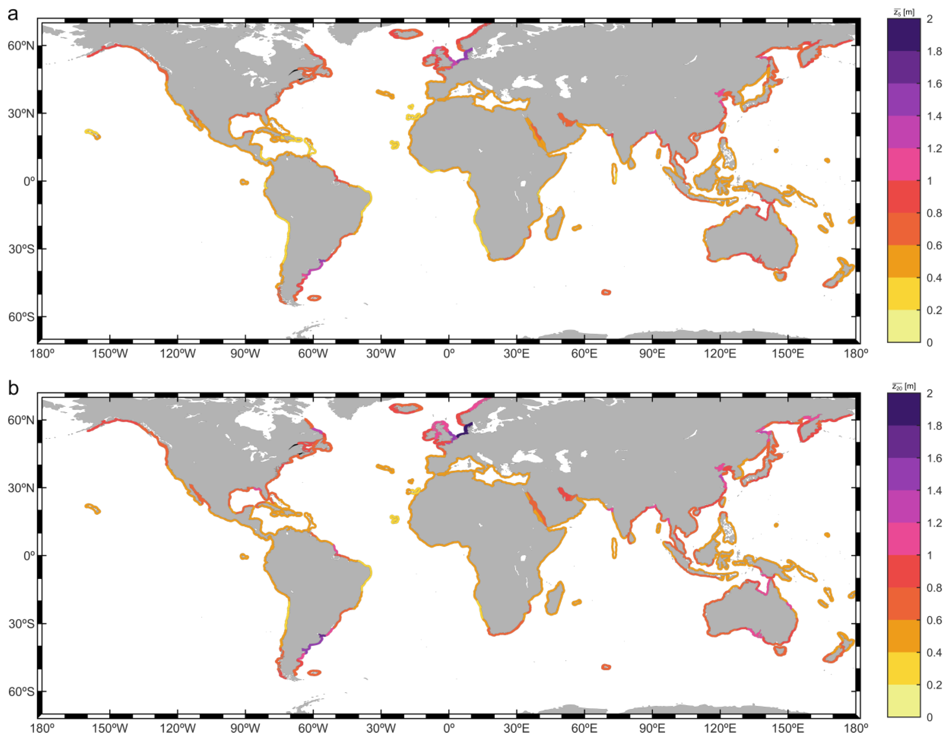
3.2. Intensity of Coastal NTR Extremes

This section describes the magnitude of NTR return levels along the global coastlines. Figure 5 depicts the 5- and 20-year NTR return levels globally ($\overline{z_5}$ and $\overline{z_{20}}$, subpanels a, b, respectively; Equation (2)). The results for all of the analyzed return periods exhibited similar spatial patterns, so for the sake of simplicity, only the results for $\overline{z_{20}}$ are described below.

Extreme NTR events impacting the eastern coast of America were more intense poleward of 40° in both hemispheres, with $\overline{z_{20}}$ values ranging from 0.6 m to 0.8 m poleward of 50°, and from 0.8 m to 1.0 m between 40° and 50°. Along subtropical and intertropical coasts, $\overline{z_{20}}$ values mostly fell between 0.4 m and 0.6 m, the only exception being the Gulf of California, where values ranged between 0.6 m and 0.8 m. The eastern coast of America generally experienced more intense NTR extremes than its western counterpart, consistently exhibiting $\overline{z_{20}}$ values greater than 0.6 m north of 30°N, even exceeding 0.8 m along some coastal areas north of 45°N. Despite the probable attenuation of NTR extremes induced by tropical cyclones (Figure 4b), the coast of the Gulf of Mexico presented significant $\overline{z_{20}}$ values. Values above 0.6 m could be observed along the entire coastline of this basin and, notably, exceeded 1 m on the east coast of Florida (USA). Coasts south of 30°S generally exceeded $\overline{z_{20}}$ values of 0.6 m, particularly between 30°S and 45°S, where highly intense NTR extreme events yielded $\overline{z_{20}}$ values over 1.4 m.

The western coasts of Europe showed a pronounced $\overline{z_{20}}$ gradient. The Atlantic coasts of Spain and Portugal, along with the southeast coast of France, exhibited $\overline{z_{20}}$ values ranging from 0.4 m to 0.8 m. In contrast, the southern coasts of the North Sea exceeded 1.4 m, with the Dutch, German, and Danish coasts in this basin reaching values over 1.8 m. African coastlines predominantly showed $\overline{z_{20}}$ values below 0.6 m, only exceeding this value on the South African coast (between 0.6 m and 0.8 m).

Along Indian Ocean coasts, two main areas stood out due to an intensity of NTR extremes. The first was the north coast of the Gulf of Bengal, with $\overline{z_{20}}$ values ranging between 0.8 m and 1.2 m. The second was the Persian Gulf, where almost the entire basin showed values between 0.8 m and 1.0 m. The south coast of Japan and most of Chinese coast presented $\overline{z_{20}}$ values above 0.8 m, also exceeding 1.2 m in some sections of the Yellow Sea. The Australian coast exhibited significant $\overline{z_{20}}$ values over 0.6 m along almost the entire coast, with particularly intense events impacting the Gulf of Carpentaria and some areas along the southern and eastern coasts, reaching values between 1.0 m and 1.2 m. The coastlines of Tasmania and South Island in New Zealand also displayed considerable magnitudes, ranging between 0.6 m and 0.8 m.

3.3. Climate Variability of Coastal ESLs

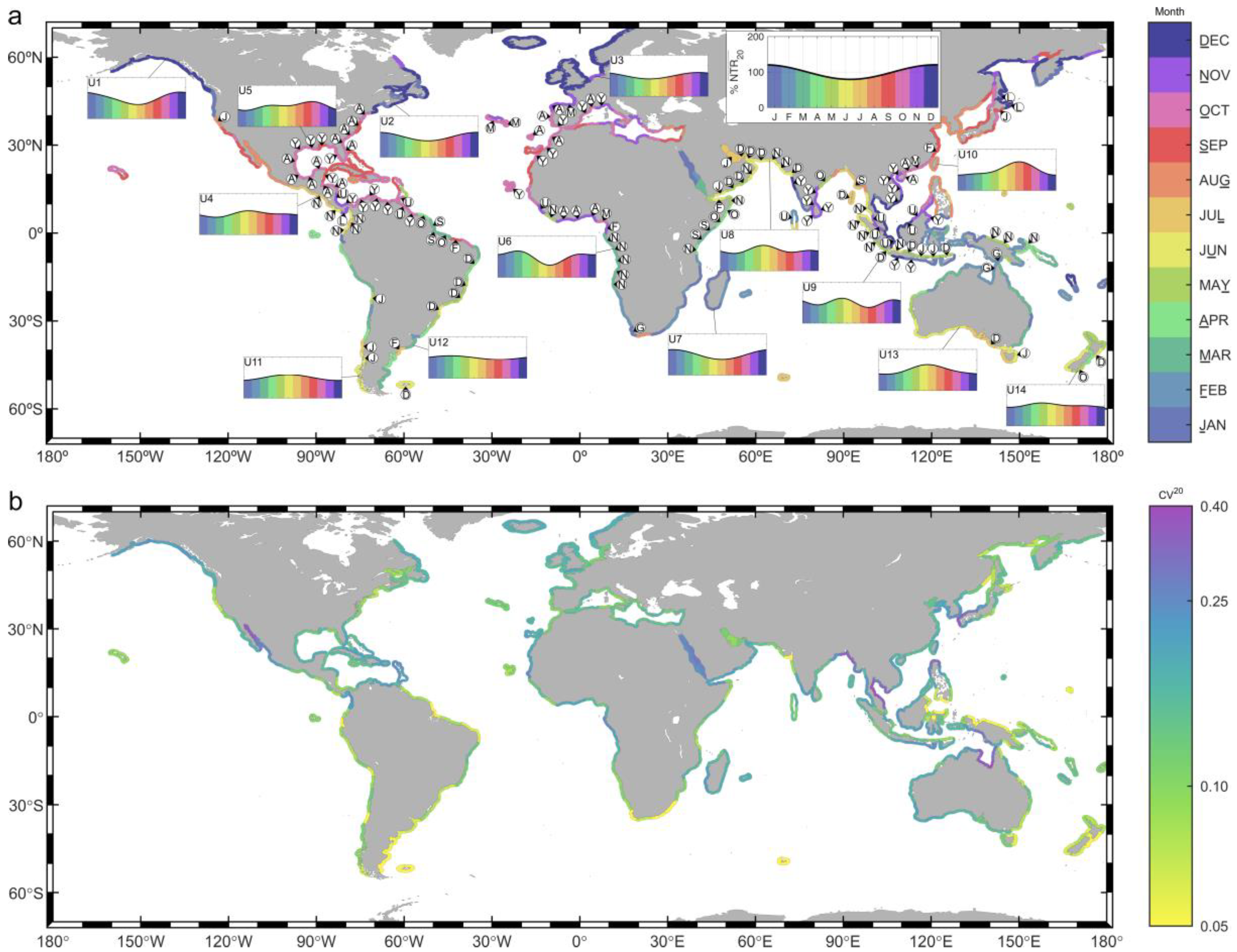
3.3.1. Intra-Annual Variability

The intensity of NTR extremes reaching the coast varies throughout the year due to the intrinsic intra-annual variability of their generating events (e.g., tropical cyclones, extratropical cyclones). The variability of extreme events within a year is depicted in Figure 6. Figure 6a shows the month with the highest probability of experiencing the highest NTR extremes (i.e., the highest return levels within a year; see Section 2.6.1). It also highlights coastal areas where NTR return levels exhibited more than one local maximum within a year, indicating that these coasts could be affected by extreme events of different geneses. The month showing this second maximum is also displayed (white circles). Additionally, the evolution of $z_{t20}$ within a year (normalized by ${\overline{x}}^{R20}$) at fourteen key coastal units (U1 to U14) along the global coastlines is presented in Figure 6b. Five of these units are in the Pacific Ocean, five are in the Atlantic Ocean, and four are in the Indian Ocean. These coastal units were selected with two primary objectives: to homogenously cover the global coastlines, and to represent distinct NTR extreme behaviors, illustrating the differences between coastal regions in terms of the shape and complexity of the intra-annual variability pattern. Coastal units where extremes have a single origin showed simpler monthly evolution patterns, characterized by a clear annual cycle (e.g., units U1–U3, U7, U11–U13). On the other hand, coasts impacted by NTR extremes of more than one origin, mostly observed in subtropical and intertropical coasts, exhibited more complex seasonal patterns (e.g., units U4–U6, U8–U9).

The primary driver of NTR extremes impacting mid to high latitude coasts are extratropical cyclones moving from west to east along the extratropical storm tracks [76,77]. These events showed a strong inter-annual variability pattern, with maximum magnitudes during the corresponding winter season in each hemisphere and minimum magnitudes during the summer. Most coastal units in these latitudes showed a single maximum within the year (U1–U3, U11–U13), corroborating the strong winter-summer pattern. Coasts north of 40°N (U1–U3) exhibited the highest probability of experiencing more extreme events from November to February, whereas the pattern in extratropical coasts in the SH was less clear. However, a significant winter dominance (from May to July) in extreme NTR occurrence could still be observed in the south coast of Chile, the south and west coasts of Australia, the southernmost part of the coast of South Africa and the coasts of New Zealand (U11–U14).

The eastern coastlines of the continents in subtropical and intertropical latitudes can be impacted by tropical cyclones [20,78]. Therefore, months within the tropical cyclone seasons (i.e., approximately from June to November in the NH and from November to April in the SH) were roughly those showing the highest NTR extreme values. The coasts of the Gulf of Mexico and the Caribbean Sea experience the highest NTR events mainly from September to November (U5), whereas along open NH tropical West Pacific coasts the highest NTR events are most likely to occur in earlier months, from July to September (U10). Moreover, all mainland coasts in the latter regions exhibited a second maximum in NTR return levels from April to May, something that was not observed on islands at the same latitudes, such as in the Caribbean islands, Taiwan, and The Philippines. In the SH, the coasts of Mozambique, Madagascar, and the Reunion and Mauritius islands showed maximum values in January and February (U7). Additionally, the northeast and southeast coasts of Australia suffer the highest events from January to April.

Notable differences were observed within the same basin, mainly depending on the orientation of the coastline. The Arabian Sea coasts are a clear example of this phenomenon. The west coast of India experiences the highest NTR events in December–January, while the highest events along the coasts of Pakistan, East Iran, and Oman occur in May–June. However, all these coasts showed a second $z_{t20}$ maximum in November–December (U8), indicating that they are likely to be affected by the same extreme events as the coast of West India. Another example is the Gulf of Guinea, where the coasts of Gabon and Angola, orientated to the west, exhibited the highest NTR events in March with a second maximum in November (U7), and the coasts of Cameroon, Nigeria, Togo, Ghana, and Ivory Coast, orientated to the south, showed the highest extremes in October–November, with a second maximum in March–April. These patterns likely reflect the effect of extreme events on all these coasts, with the dominance alternating based on coastline orientation.

Figure 6b depicts the strength of the intra-annual variability measured through the CV²⁰ metric (Equation (10)). Generally, coasts poleward of 35° in the NH showed higher CV²⁰ values compared to their SH counterparts. For example, the coast of the Gulf of Alaska, the northernmost part of the northeastern American coast, and the northwestern European coast showed CV²⁰ values ranging between 0.10 and 0.25, whereas the southernmost part of the Chilean and Argentinean coasts and the coast of South Africa showed CV²⁰ values lower than 0.15. This discrepancy reflects a more pronounced seasonality in NH extratropical coasts with respect to the SH, as can also be observed by comparing the intra-annual evolution of $z_{t20}$ at coastal units in the extratropical NH (U1-U3 in Figure 6a) and the extratropical SH (U11-U13 in Figure 6a). Additionally, it is noteworthy the low CV²⁰ values (0.05 to 0.15) observed in the coasts of Uruguay and Argentina and the south coast of the North Sea, coastal regions affected by very high NTR extremes (Figure 5), which suffer a sustained significant intensity during the whole year.

There is significant heterogeneity in the CV²⁰ pattern in intertropical and subtropical coasts, even within the same basin. For example, the coasts in the Arabian Sea exhibited CV²⁰ values ranging between 0.05 and 0.25. The coasts most affected by extremes induced by tropical cyclones showed significant CV²⁰ values, roughly from 0.10 to 0.25 on coasts in the Gulf of Mexico and Caribbean Islands (U5 in Figure 6a), and from 0.15 to 0.35 on NH tropical West Pacific coasts (U10 in Figure 6a). These results highlight the high NTR magnitudes induced by tropical cyclones compared to those present the rest of the year.

Finally, it is worth noting the high CV²⁰ values on coasts in semi-enclosed basins, such as the Gulf of California, the Gulf of Carpentaria, and the Red Sea. The latter stands out for being affected by NTR extremes of great magnitude (Figure 5).

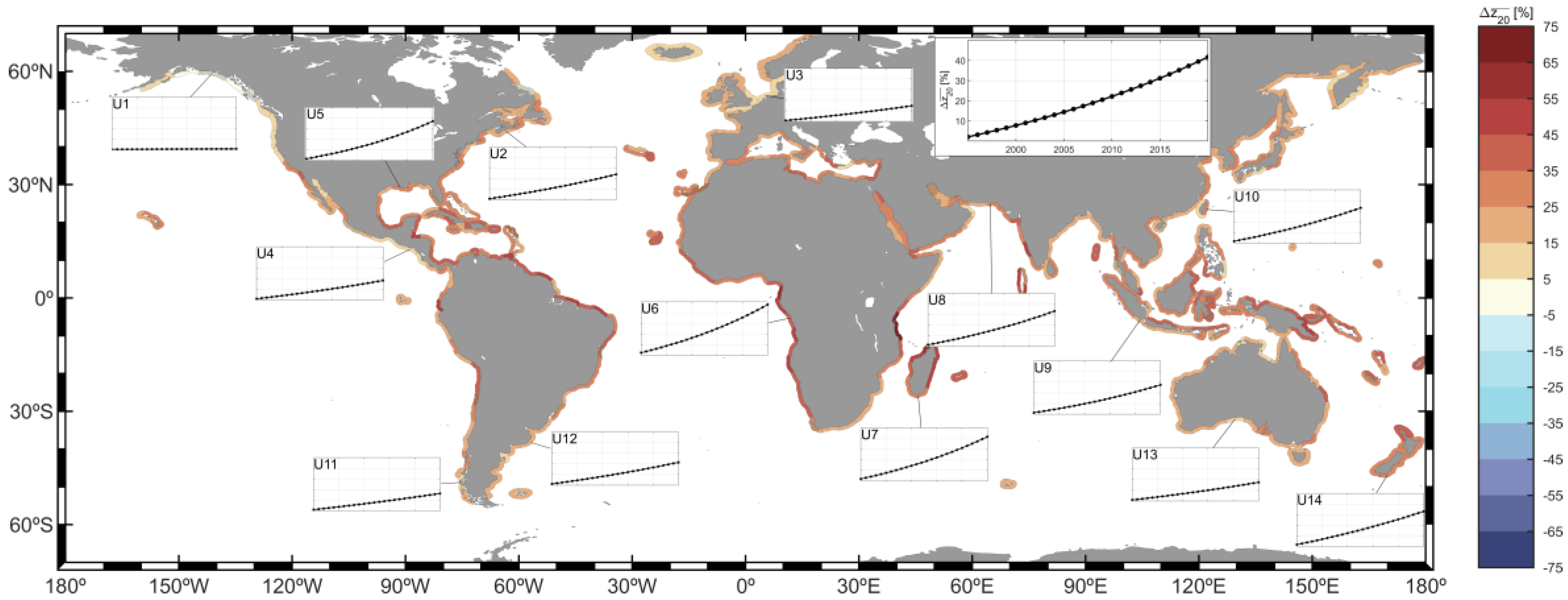
3.3.2. Long-Term Trends

Figure 7 presents the long-term variability (i.e., long-term trends) of $\overline{z_{20}}$ along the global coastlines (Equation (11)) and also examines whether the inclusion of the trend to model the behavior of NTR extremes was significant at a 95% confidence level (Equation (4)). The results revealed a robust positive trend in $\overline{z_{20}}$, with most coastal units exhibiting an increasing trend, and more than 95% of them showing significant trends. Low-robust trends were mainly found in the coast of the Gulf of Alaska. These findings are consistent with previous studies, which suggested that mean sea level rise is the primary driver of changes in ESLs [11,12,15].

The strongest trends in $\overline{z_{20}}$ were found in five main coastal regions: the southwestern African coast; the coasts of North Madagascar, North Mozambique, and Tanzania; the coasts of Papua New Guinea, Indonesia, and the Solomon Islands; the coast of West India; and the coast of Brazil. These regions showed increases in $\overline{z_{20}}$ greater than 35%, with some coastal units experiencing increases of more than 50%. On the other hand, the Atlantic European coasts, the southernmost part of the Chilean coast, the Argentinean and Uruguayan coasts, the northwestern coasts of America, and the south, west, and north coasts of Australia showed the lowest increases in $\overline{z_{20}}$, ranging between 5% and 25%.

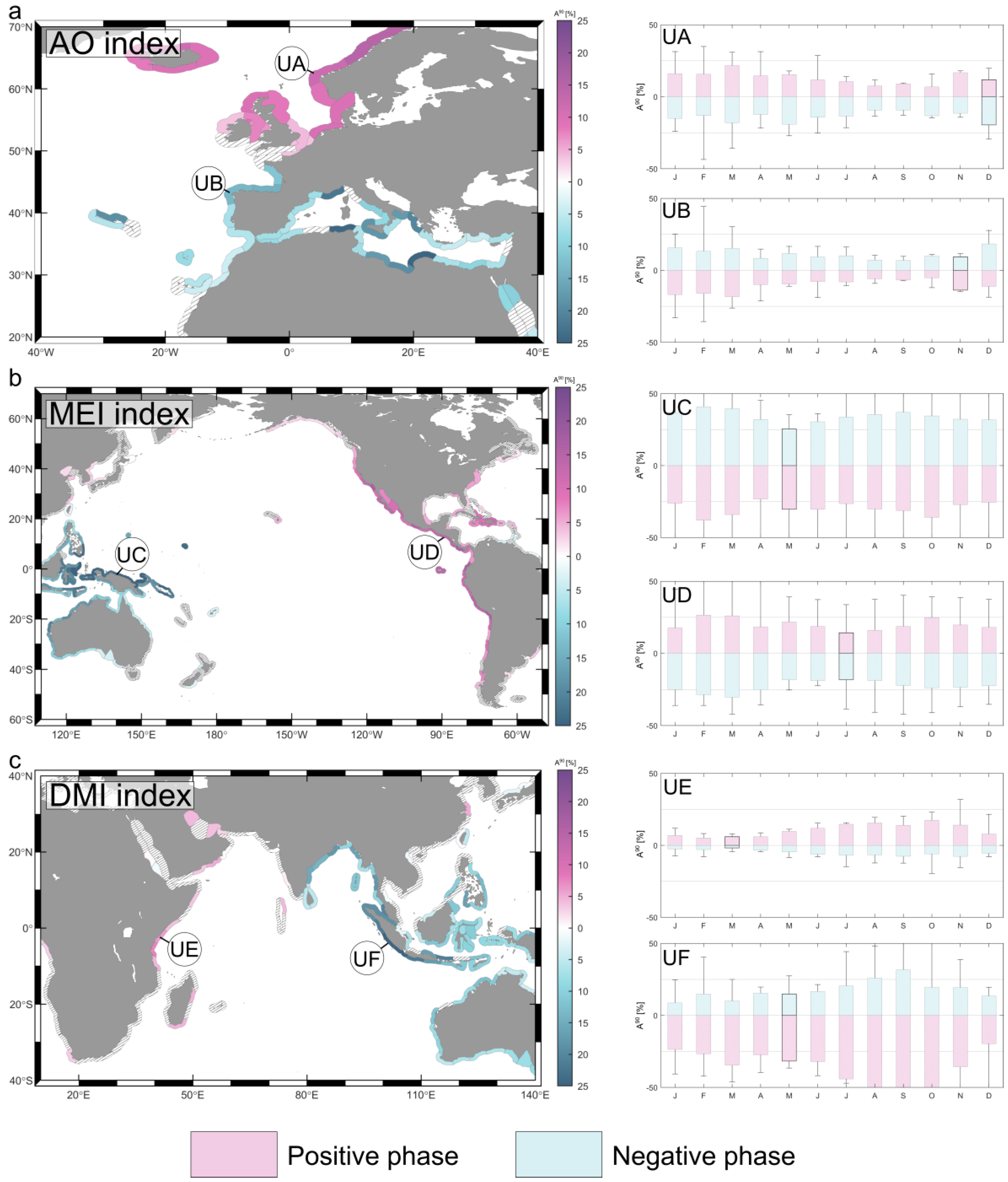
3.3.3. Inter-Annual Variability

Inter-annual variability is present in NTR extreme events. By incorporating climate teleconnection indices into the extreme statistical model (Equation (5)), we could examine the individual effect of climate teleconnection patterns on the intensity of NTR extremes. Figure 8 depicts the relationship between three teleconnection indices and monthly NTR return levels for three specific regions: AO for North Atlantic Ocean coasts, MEI for Pacific coasts, and DMI for Indian Ocean coasts (panels a-c, respectively). The maps in Figure 8 show $A^{90}$ (Equation (12)) for the month with the highest probability of showing the highest NTR extremes (see Figure 6a), where the color indicates the phase in which this happens (pink for positive phase; blue for negative phase). In addition, it shows the monthly impact of the inter-annual variability at six coastal units, two for each climate index (coastal units UA-UF). For each coastal unit, monthly boxes represent $A^{10}$ (lower bound) and $A^{90}$ (upper bound), calculated as indicated in Equation (12), whereas the whiskers represent the maximum and minimum monthly anomalies during the period of analysis. We also examined the statistical robustness of introducing the teleconnection index covariate into the statistical model (Equation (5)), considering the results to be robust when the statistical significance was greater than 95%.

The impact of the Arctic Oscillation teleconnection pattern (AO index) on NTR return levels in the North Atlantic coasts is shown in Figure 8a. A strong correlation was found between the positive phase of the AO index and NTR extreme events along the northwestern coasts of Europe (pink colors in Figure 8). This indicated a higher probability of experiencing higher NTR extreme events during this phase. The AO index, which is highly correlated with the NAO index [79], is closely related with the position of the NH extratropical storm track in the Atlantic Ocean. During the AO positive phase, storms tend to reach poleward coastlines, which explains the positive correlation found in these coasts. Increases in $z_{t20}$ over 15% during this phase with respect to the neutral phase during the stormiest month, measured through $A^{90}$ metric, were found in the western Norwegian coast and the coast of Iceland. The coasts of the North Sea and the north coasts of the British Islands also showed increases above 10%. The specific analysis conducted at UA showed that, from January to April, $A^{90}$ presented values over 15% during the AO positive phase. Moreover, the results indicate that increases reached values over 30% during these months in the 28-year period analyzed (whiskers of the bar plots).

Conversely, during the AO negative phase, storms tend to make landfall more to the south, resulting in a negative correlation with NTR extremes along the southwestern coasts of Europe, namely those in the Gulf of Biscay, the Atlantic coasts of the Iberian Peninsula, and the Mediterranean coasts. Increases over 10% were observed during this phase along these coasts, except for the easternmost Mediterranean coasts, where the increases were lighter. Coastal unit UB, in the northwestern coast of Spain, showed the strongest interannual variability from December to March. During these months, $A^{90}$ showed values over 10% for the negative AO phase. Moreover, increases over 25% were observed for years with very intense AO index values.

The effect of ENSO teleconnection pattern on the inter-annual variability of NTR extremes was analyzed through the MEI index, as depicted in Figure 8b. Positive values of this index are related to El Niño phase and negative values to La Niña phase. A robust influence of ENSO phenomenon in NTR return levels could be observed in intertropical and subtropical Pacific coasts, with a clear dipole pattern: positive MEI correlations (i.e., higher extremes during El Niño phase) along eastern Pacific Ocean coasts and negative correlations (i.e., higher extremes during La Niña phase) along western Pacific Ocean coasts. The most intense effect of El Niño phase on the magnitude of NTR extremes was observed along the Pacific coasts of Mexico, Guatemala, El Salvador, Honduras, Nicaragua, Costa Rica, and Panama. Values of $A^{90}$ exceeding 20% were observed along these coasts during this phase. A detailed analysis at UD revealed a very strong inter-annual variability throughout the whole year, exhibiting significant increases during El Niño phase and significant decreases during La Niña phase. In this regard, although $A^{90}$ was below 30% for every month, the analysis of the 28-year period indicated that increases of over 50% in $z_{t20}$ during this phase with respect to the neutral phase were occasionally reached. The intensification of NTR extremes during El Niño phase extended to the entire western coast of America, namely from Alaska (USA) to Chile, albeit showing lower anomalies in poleward latitudes.

Extreme events of NTR reaching the coasts of Papua New Guinea, The Philippines, Indonesia, North Sumatra, North Java, East Vietnam, and Northeast Australia showed a robust correlation with La Niña phase. Increases over 25% could be observed among these coasts in the stormiest month during La Niña phase in comparison with the neutral phase. An assessment at UC exhibited a very strong inter-annual variability, even more than along the eastern Pacific coasts. Our results showed $A^{90}$ over 25% during La Niña phase for every month, reaching values beyond 50% for intense La Niña events. As expected, during El Niño phase, a significant decrease in NTR was observed throughout the year. Further, note that this negative pattern extended to the Indian ocean along the south coasts of Sumatra and Java, the north, west, and south coasts of Australia, and the coasts of the Bay of Bengal.

The effect of the Indian Ocean Dipole climate pattern on NTR extremes was examined using the DMI index (Figure 8c). A dipole pattern along Indian coasts was observed, characterized by a correlation between NTR extremes with the negative phase of DMI along eastern Indian Ocean coasts and the opposite along western Indian Ocean coasts. Nevertheless, it is worth mentioning that the former was stronger than the latter. The intensity of NTR extremes along the south, east, and north Australian coasts, the south coasts of Sumatra and Java, and the coasts in the Bay of Bengal showed $A^{90}$ values above 25% during the DMI negative phase. Consistently, the results at UF showed that increases in $z_{t20}$ during the negative phase reached values above 30% from July to November.

On the other hand, along the coasts of Somalia, Kenya, Tanzania, the south coast of Madagascar, and the south coast of Oman, a robust positive correlation with DMI index was observed. In general, increases along these coasts during the stormiest month did not exceed 10%. At coastal unit UE, the results showed $A^{90}$ values of over 10% during the period of analysis from June to December. Decreases during the negative phase of DMI index were significantly lower than the increases experienced during the positive phase.

3.3.4. Extreme Variability Dominance

After exploring the variability in NTR return levels on individual time scales, we then qualitatively assessed the importance of each time-scale variability along the global coastlines during the 1995–2020 period. We aimed to determine the relative importance of changes in NTR return levels within the year, from one year to another, and over the long-term within the analyzed period.

The relative importance of the three variability time scales explored in this study is depicted in Figure 9, for the same regions shown in Figure 8. For each region, inter-annual variability was analyzed, considering the influence of a different climate teleconnection pattern (indicated in the upper-left corner of each panel). Along the Western European and Mediterranean coasts, there was a split dominance between the three variability time scales (Figure 9a). However, a more pronounced dominance of intra-annual variability was observed along the coasts of the British Isles, Iceland, and Norway. This indicated that, for example, variations in NTR return levels during the 1995–2020 period along the coasts of Iceland were stronger within a single year than over the entire period of analysis.

The Pacific coastal regions, strongly affected by the ENSO phenomenon, exhibited notable differences (Figure 9b). The coast of South America south of 10°S revealed a split dominance between the three time scales, except for the southernmost part, where trends and intra-annual variability dominated over inter-annual changes. The variability along the eastern Pacific coasts from 10°S to 20°N was dominated by inter-annual changes induced by the ENSO phenomenon. A split dominance among the three time scales extended northward up to 40°N, with the only exception of the Gulf of California, mostly due to intra-annual variations. The coast of the Gulf of Alaska, the coastal region exhibiting the lowest trends (Figure 7), showed a clear dominance of intra-annual variability, with a minor contribution of inter-annual variations. The coasts of East Asia presented a clear dominance of intra-annual variability, followed by the long-term trends. The inter-annual variability dominated along a significant part of the Pacific coasts of the Maritime Continent, with long-term trends being the least important contributor. The main variability scale along the north coast of Australia was found to be the intra-annual, followed by the inter-annual. Lastly, the east coast of Australia showed a split dominance between trends and intra-annual variability.

Finally, the Indian Ocean coasts were shown to be mostly governed by intra-annual and long-term variations (Figure 9c). The most remarkable exceptions were the southern coasts of Sumatra and Java, where the changes related to the inter-annual variability were the most important.

4. Conclusions and Discussion

Coastal ESLs are an important subject of analysis, due to the severe impacts they may cause in coastal areas. Despite the use of tide gauge and modeling data becoming more common in the study of these events, improvements in the accuracy of altimetry data and its current availability period of over thirty years mean that such data could serve as an alternative to address multiple climatic-based purposes, always with consideration of the limitations of such an approach. In this context, we have explored the use of this data source to examine the climate variability of coastal ESLs. The present study was intended to maximize the strengths of altimetry data in terms of the climate behavior and escape from its main weaknesses, i.e., the irregular time and spatial sampling and potential underestimation of extremes.

In particular, we have focused on the NTR component of sea level. No altimetry based NTR product is openly available, so a complete dataset using a global, multi-platform, inter-calibrated along-track altimetry product covering the period from 1993 to 2020 was built.

The analysis was conducted worldwide on more than 400 coastal units that covered the global coastlines uniformly (Figure 1). The analysis focused on the climate variability of coastal NTR extremes with very low probability of occurrence (i.e., magnitudes associated to return periods). To achieve this, a non-stationary EVA was conducted at each coastal unit using a time varying GEVD statistical model that employed monthly maxima as input. The extreme variability was introduced in the model through the location parameter as a parametric function. We considered variations on three time scales (Equation (6)), namely: intra-annual, by combining sine functions; inter-annual, by introducing teleconnection indices as covariates; and long-term trends, by fitting an exponential function.

In order to provide robustness to the results, an extensive validation was done by comparison against TG data. We should note that this comparison could be unfair at some locations, as altimetry data are mostly measured offshore, and TG data are frequently affected by local processes due to interactions with the sea floor and coastal features. Additionally, despite comparable NTR samples from TG and altimetry being thoroughly selected at each TG location to conduct the validation, inherent spatiotemporal inconsistency between the two data sources is inevitable. Altimetry measurements will always be made at different locations than the TG and with a different temporal resolution, which may translate into differences in the magnitudes measured and delays in the timing of extreme events. Despite this, our validation results demonstrated the value of altimetry data in terms of reproducing the variability of NTR return levels (Figure 4). The magnitude of extremes was also reasonably well captured. The accuracy of the altimetry-based NTR dataset was unavoidably affected by the corrections applied to altimetry measurements (e.g., tidal corrections) and was subjected to further improvements in coastal regions. The poorest results were obtained, as expected, in coastal regions affected by extreme events generated by tropical cyclones. Such underestimates mean that the use of altimetry data within these regions should be done with the necessary critical assessments to avoid misleading results. It is relevant to highlight that the underestimation of ESLs induced by tropical cyclones is not exclusive to altimetry, as results from numerical models also experience similar issues within these regions [42]. In general, our results provide confidence in the subsequent climate variability analysis conducted along the global coastlines. Moreover, given the excellent representation of the climate variability based on altimetry data and the probable underestimation in certain tropical regions, our results were provided and evaluated as relative magnitudes whenever possible, hence concentrating on variability and avoiding, at least partially, the influence of underestimation.

Prior to exploring the variability of NTR extremes, the magnitudes of events with return periods of 5 to 20 years were analyzed (Figure 5). First, it is relevant to mention that the global spatial distribution of the magnitudes was consistent with findings from previous studies [33,42]. We observed that the coast of the North Sea and the coasts of Argentina and Uruguay suffered the highest NTR events, with the former exceeding 1.8 m and the latter 1.4 m for $\overline{z_{20}}$. Despite the magnitude of tropical cyclones not being fully captured, coasts impacted by this type of storms, such as those in the Gulf of Mexico, China, south Japan, and the Gulf of Carpentaria, showed notably high NTR return levels, all exceeding 1 m for $\overline{z_{20}}$.

Our assessment of extreme intra-annual variability indicated that coasts in extratropical latitudes exhibited a clear winter–summer variability pattern, experiencing the highest NTR events during the corresponding winter month in each hemisphere (Figure 6a). Additionally, our results suggested that this seasonality is more pronounced in the NH than in the SH. In contrast, there was significant heterogeneity in the most probable month for the highest extremes in subtropical and intertropical coasts. Many of these coasts did not present a simple intra-annual variability pattern (e.g., winter-summer variability), but rather, showed two distinct storm periods, likely due to extremes of different origins. For example, the coast in the Gulf of Mexico experiences the impact of the most intense NTR extremes during the TC season, particularly in September and October, and exhibits another maximum between May and April (U5 in Figure 6a). Meanwhile, coasts in the southwestern tropical Pacific affected by tropical cyclones experience the most intense NTR events earlier than in the Atlantic, mostly in August and September (U10 in Figure 6a).

The long-term variability assessment revealed a clear increasing pattern in NTR return levels between 1995 and 2020 along the global coastlines (Figure 7). The only coastal region showing almost null increases (and low statistical robustness) was the northwestern coast of America. These results reinforce the findings from previous studies stating this to be the main driver of the changing ESLs due to climate change [11,80]. Moreover, MSLR very likely also explains the fact that we found significant trends (95% confidence level) in over 95% of the coastal units analyzed. Relative changes higher than 50% were observed along some parts of the southwestern African coast and Mozambican channel.

The inter-annual variability of NTR extremes was analyzed based on the influence of three climate teleconnection patterns (Figure 8): the Arctic Oscillation pattern through the AO index; the ENSO phenomenon pattern through the MEI index; and the Indian Ocean Dipole pattern through the DMI index. The findings revealed a strong correlation between AO and NTR extremes. During its positive phase, the northwestern coasts of Europe experienced over a 20% increase in NTR return levels with respect to the neutral phase. On the other hand, the negative phase of AO relates to an increase in NTR extremes along the southwestern coasts of Europe, including the Gulf of Biscay, the Atlantic coasts of the Iberian Peninsula, and the western Mediterranean coasts, with values over 10%. A clear dipole pattern was observed in relation to ENSO, with El Niño phase resulting in NTR increases of over 25% along the eastern Pacific coasts, and La Niña phase leading to intensified NTR extremes along the western Pacific coasts. Similarly, the IOD pattern related to the variability of NTR extremes along the Indian Ocean coasts, exhibiting a dipole pattern in which its positive phase induced increases in NTR return levels along the western coasts of the Indian basin and the negative phase doing so for the eastern coasts.

An analysis of the relative influence of the three time variability scales explored on the variations experienced by NTR return levels between 1995 and 2020 was conducted (Figure 9). The coasts of the British Isles, Iceland, and Norway showed a clear dominance of intra-annual variability, with a fluctuating secondary dominance of long-term trends and inter-annual variability (AO influence). Pacific coastal regions, notably influenced by the ENSO phenomenon, exhibited varying dominance across time scales, with intra-annual variability controlling the return levels variability in regions such as East Asia and the Gulf of Alaska. The ENSO phenomenon, however, dominated along most of the Pacific coasts of the Maritime Continent and Central America. Indian Ocean coasts were predominantly governed by intra-annual and long-term variations, but regions such as the southern coasts of Sumatra and Java were shown to be controlled by inter-annual variability.

Despite the above findings, there is still room for improvement in terms of magnitude accuracy, and further uncertainty analysis are required. Nonetheless, the results presented here provide a reliable indication of the potential value of altimetry data in climate studies, particularly those focusing on ESLs. Altimetry data have been proven to present very good accuracy in terms of capturing the climate variability extreme events, offering a very useful database to explore the behavior of extremes on different time and spatial scales. However, if this information is intended to be used for local assessments, the inherent limitations of the present study must be considered, especially given the pivotal role played by the magnitude of the extremes. Currently, the accuracy of altimeters in coastal areas, in conjunction with the time period covered (~30 years) and the irregular time and spatial sampling, make altimetry data useful for providing preliminary information about the magnitude of extremes reaching specific coastal regions. Nevertheless, the promising results presented here suggest that the extension of this database over time will maximize its main strength, i.e., continuous global coverage, and minimize its main weakness, i.e., irregular sampling (i.e., along track sampling). Furthermore, as the accuracy of coastal altimetry data increases and data availability improves, it is likely that the characterization of ESL behavior will be progressively conducted on more localized coastal scales. This is particularly beneficial in regions where in situ information and numerical modeling capacity are either limited or unavailable.

References

1. Losada, I.J.; Toimil, A.; Muñoz, A.; Garcia-Fletcher, A.P.; Diaz-Simal, P. A Planning Strategy for the Adaptation of Coastal Areas to Climate Change: The Spanish Case. Ocean. Coast. Manag. 2019, 182, 104983. [Google Scholar] [CrossRef]
2. Rueda, A.; Vitousek, S.; Camus, P.; Tomás, A.; Espejo, A.; Losada, I.J.; Barnard, P.L.; Erikson, L.H.; Ruggiero, P.; Reguero, B.G.; et al. A Global Classification of Coastal Flood Hazard Climates Associated with Large-Scale Oceanographic Forcing /704/106/829/2737/704/4111/141/129 Article. Sci. Rep. 2017, 7, 5038. [Google Scholar] [CrossRef] [PubMed]
3. Bromirski, P.D.; Cayan, D.R.; Helly, J.; Wittmann, P. Wave Power Variability and Trends across the North Pacific. J. Geophys. Res. Ocean. 2013, 118, 6329–6348. [Google Scholar] [CrossRef]
4. Miao, Q.; Yue, X.; Yang, J.; Wang, Z.; Xu, S.; Yang, Y.; Chu, S. Characteristics Analysis and Risk Assessment of Extreme Water Levels Based on 60-Year Observation Data in Xiamen, China. J. Ocean. Univ. China 2022, 21, 315–322. [Google Scholar] [CrossRef]
5. Yin, D.; Muñoz, D.F.; Bakhtyar, R.; Xue, Z.G.; Moftakhari, H.; Ferreira, C.; Mandli, K. Extreme Water Level Simulation and Component Analysis in Delaware Estuary during Hurricane Isabel. J. Am. Water Resour. Assoc. 2022, 58, 19–33. [Google Scholar] [CrossRef]
6. Kates, R.W.; Colten, C.E.; Laska, S.; Leatherman, S.P. Reconstruction of New Orleans after Hurricane Katrina: A Research Perspective. Proc. Natl. Acad. Sci. USA 2006, 103, 14653–14660. [Google Scholar] [CrossRef] [PubMed]
7. Toimil, A.; Losada, I.J.; Hinkel, J.; Nicholls, R.J. Using Quantitative Dynamic Adaptive Policy Pathways to Manage Climate Change-Induced Coastal Erosion. Clim. Risk Manag. 2021, 33, 100342. [Google Scholar] [CrossRef]
8. Coles, S. An Introduction to Statistical Modeling of Extreme Values, 1st ed.; Springer: London, UK, 2001. [Google Scholar]
9. Alves, B.; Angnuureng, D.B.; Morand, P.; Almar, R. A Review on Coastal Erosion and Flooding Risks and Best Management Practices in West Africa: What Has Been Done and Should Be Done. J. Coast. Conserv. 2020, 24, 38. [Google Scholar] [CrossRef]
10. Toimil, A.; Losada, I.J.; Nicholls, R.J.; Dalrymple, R.A.; Stive, M.J.F. Addressing the Challenges of Climate Change Risks and Adaptation in Coastal Areas: A Review. Coast. Eng. 2020, 156, 103611. [Google Scholar] [CrossRef]
11. Menéndez, M.; Woodworth, P.L. Changes in Extreme High Water Levels Based on a Quasi-Global Tide-Gauge Data Set. J. Geophys. Res. Ocean. 2010, 115. [Google Scholar] [CrossRef]
12. Wahl, T.; Haigh, I.D.; Nicholls, R.J.; Arns, A.; Dangendorf, S.; Hinkel, J.; Slangen, A.B.A. Understanding Extreme Sea Levels for Broad-Scale Coastal Impact and Adaptation Analysis. Nat. Commun. 2017, 8, 16075. [Google Scholar] [CrossRef] [PubMed]
13. Cid, A.; Menéndez, M.; Castanedo, S.; Abascal, A.J.; Méndez, F.J.; Medina, R. Long-Term Changes in the Frequency, Intensity and Duration of Extreme Storm Surge Events in Southern Europe. Clim. Dyn. 2016, 46, 1503–1516. [Google Scholar] [CrossRef]
14. Männikus, R.; Soomere, T.; Viška, M. Variations in the Mean, Seasonal and Extreme Water Level on the Latvian Coast, the Eastern Baltic Sea, during 1961–2018. Estuar. Coast. Shelf Sci. 2020, 245, 106827. [Google Scholar] [CrossRef]
15. Marcos, M.; Woodworth, P.L. Spatiotemporal Changes in Extreme Sea Levels along the Coasts of the North Atlantic and the Gulf of Mexico. J. Geophys. Res. Ocean. 2017, 122, 7031–7048. [Google Scholar] [CrossRef]
16. Méndez, F.J.; Menéndez, M.; Luceño, A.; Losada, I.J. Analyzing Monthly Extreme Sea Levels with a Time-Dependent GEV Model. J. Atmos. Ocean. Technol. 2007, 24, 894–911. [Google Scholar] [CrossRef]
17. Menendez, M.; Mendez, F.J.; Losada, I.J. Forecasting Seasonal to Interannual Variability in Extreme Sea Levels. ICES J. Mar. Sci. 2009, 66, 1490–1496. [Google Scholar] [CrossRef]
18. Zhang, W.; Yan, Y.; Zheng, J.; Li, L.; Dong, X.; Cai, H. Temporal and Spatial Variability of Annual Extreme Water Level in the Pearl River Delta Region, China. Glob. Planet. Chang. 2009, 69, 35–47. [Google Scholar] [CrossRef]
19. Thompson, P.R.; Mitchum, G.T.; Vonesch, C.; Li, J. Variability of Winter Storminess in the Eastern United States during the Twentieth Century from Tide Gauges. J. Clim. 2013, 26, 9713–9726. [Google Scholar] [CrossRef]
20. Wahl, T.; Chambers, D.P. Evidence for Multidecadal Variability in US Extreme Sea Level Records. J. Geophys. Res. Ocean. 2015, 120, 1527–1544. [Google Scholar] [CrossRef]
21. Owens, B.F.; Landsea, C.W. Assessing the Skill of Operational Atlantic Seasonal Tropical Cyclone Forecasts. Weather. Forecast. 2003, 18, 45–54. [Google Scholar] [CrossRef]
22. Rogers, D.; Tsirkunov, V. Costs and Benefits of Early Warning Systems. 2011. Available online: https://www.preventionweb.net/english/hyogo/gar/2011/en/bgdocs/Rogers_&_Tsirkunov_2011.pdf (accessed on 30 January 2024).
23. Madireddy, M.; Kumara, S.; Medeiros, D.J.; Shankar, V.N. Leveraging Social Networks for Efficient Hurricane Evacuation. Transp. Res. Part. B Methodol. 2015, 77, 199–212. [Google Scholar] [CrossRef]
24. Swamy, R.; Kang, J.E.; Batta, R.; Chung, Y. Hurricane Evacuation Planning Using Public Transportation. Socioecon. Plann Sci. 2017, 59, 43–55. [Google Scholar] [CrossRef]
25. Semedo, A.; Vettor, R.; Breivik; Sterl, A.; Reistad, M.; Soares, C.G.; Lima, D. The Wind Sea and Swell Waves Climate in the Nordic Seas. Ocean. Dyn. 2015, 65, 223–240. [Google Scholar] [CrossRef]
26. Gillett, N.P.; Kell, T.D.; Jones, P.D. Regional Climate Impacts of the Southern Annular Mode. Geophys. Res. Lett. 2006, 33. [Google Scholar] [CrossRef]
27. Tan, Y.; Zhang, W.; Feng, X.; Guo, Y.; Hoitink, A.J.F. Storm Surge Variability and Prediction from ENSO and Tropical Cyclones. Environ. Res. Lett. 2023, 18, 024016. [Google Scholar] [CrossRef]
28. Masson-Delmotte, V.; Zhai, P.; Pirani, A.; Connors, S.L.; Péan, C.; Berger, S.; Caud, N.; Chen, Y.; Goldfarb, L.; Gomis, M.I.; et al. IPCC, 2021: Climate Change 2021: The Physical Science Basis; Cambridge University Press: Cambridge, UK, 2021. [Google Scholar]
29. Cazenave, A.; Dieng, H.B.; Meyssignac, B.; Von Schuckmann, K.; Decharme, B.; Berthier, E. The Rate of Sea-Level Rise. Nat. Clim. Chang. 2014, 4, 358–361. [Google Scholar] [CrossRef]
30. Nicholls, R.J.; Cazenave, A. Sea-Level Rise and Its Impact on Coastal Zones. Science (1979) 2010, 328, 1517–1520. [Google Scholar] [CrossRef] [PubMed]
31. Vousdoukas, M.I.; Mentaschi, L.; Voukouvalas, E.; Verlaan, M.; Feyen, L. Extreme Sea Levels on the Rise along Europe’s Coasts. Earths Future 2017, 5, 304–323. [Google Scholar] [CrossRef]
32. Vousdoukas, M.I.; Mentaschi, L.; Voukouvalas, E.; Verlaan, M.; Jevrejeva, S.; Jackson, L.P.; Feyen, L. Global Probabilistic Projections of Extreme Sea Levels Show Intensification of Coastal Flood Hazard. Nat. Commun. 2018, 9, 2360. [Google Scholar] [CrossRef]
33. Muis, S.; Apecechea, M.I.; Dullaart, J.; de Lima Rego, J.; Madsen, K.S.; Su, J.; Yan, K.; Verlaan, M. A High-Resolution Global Dataset of Extreme Sea Levels, Tides, and Storm Surges, Including Future Projections. Front. Mar. Sci. 2020, 7, 263. [Google Scholar] [CrossRef]
34. Muis, S.; Aerts, J.C.J.H.; José, J.A.; Dullaart, J.C.; Duong, T.M.; Erikson, L.; Haarsma, R.J.; Apecechea, M.I.; Mengel, M.; Le Bars, D.; et al. Global Projections of Storm Surges Using High-Resolution CMIP6 Climate Models. Earths Future 2023, 11, e2023EF003479. [Google Scholar] [CrossRef]
35. Kirezci, E.; Young, I.R.; Ranasinghe, R.; Muis, S.; Nicholls, R.J.; Lincke, D.; Hinkel, J. Projections of Global-Scale Extreme Sea Levels and Resulting Episodic Coastal Flooding over the 21st Century. Sci. Rep. 2020, 10, 11629. [Google Scholar] [CrossRef]
36. Arns, A.; Wahl, T.; Haigh, I.D.; Jensen, J.; Pattiaratchi, C. Estimating Extreme Water Level Probabilities: A Comparison of the Direct Methods and Recommendations for Best Practise. Coast. Eng. 2013, 81, 51–66. [Google Scholar] [CrossRef]
37. Haigh, I.D.; MacPherson, L.R.; Mason, M.S.; Wijeratne, E.M.S.; Pattiaratchi, C.B.; Crompton, R.P.; George, S. Estimating Present Day Extreme Water Level Exceedance Probabilities around the Coastline of Australia: Tropical Cyclone-Induced Storm Surges. Clim. Dyn. 2014, 42, 139–157. [Google Scholar] [CrossRef]
38. Lambert, E.; Rohmer, J.; Le Cozannet, G.; Van De Wal, R.S.W. Adaptation Time to Magnified Flood Hazards Underestimated When Derived from Tide Gauge Records. Environ. Res. Lett. 2020, 15, 074015. [Google Scholar] [CrossRef]
39. Adebisi, N.; Balogun, A.L.; Min, T.H.; Tella, A. Advances in Estimating Sea Level Rise: A Review of Tide Gauge, Satellite Altimetry and Spatial Data Science Approaches. Ocean. Coast. Manag. 2021, 208, 105632. [Google Scholar] [CrossRef]
40. Denys, P.H.; Beavan, R.J.; Hannah, J.; Pearson, C.F.; Palmer, N.; Denham, M.; Hreinsdottir, S. Sea Level Rise in New Zealand: The Effect of Vertical Land Motion on Century-Long Tide Gauge Records in a Tectonically Active Region. J. Geophys. Res. Solid. Earth 2020, 125, e2019JB018055. [Google Scholar] [CrossRef]
41. Tebaldi, C.; Strauss, B.H.; Zervas, C.E. Modelling Sea Level Rise Impacts on Storm Surges along US Coasts. Environ. Res. Lett. 2012, 7, 014032. [Google Scholar] [CrossRef]
42. Muis, S.; Verlaan, M.; Winsemius, H.C.; Aerts, J.C.J.H.; Ward, P.J. A Global Reanalysis of Storm Surges and Extreme Sea Levels. Nat. Commun. 2016, 7, 11969. [Google Scholar] [CrossRef]
43. Zhang, H.; Sheng, J. Examination of Extreme Sea Levels Due to Storm Surges and Tides over the Northwest Pacific Ocean. Cont. Shelf Res. 2015, 93, 81–97. [Google Scholar] [CrossRef]
44. Mo, D.; Li, J.; Hou, Y.; Hu, P. Modeling the Sea Level Response of the Northern East China Sea to Different Types of Extratropical Cyclones. J. Geophys. Res. Ocean. 2023, 128, e2022JC018728. [Google Scholar] [CrossRef]
45. Cipollini, P.; Calafat, F.M.; Jevrejeva, S.; Melet, A.; Prandi, P. Monitoring Sea Level in the Coastal Zone with Satellite Altimetry and Tide Gauges. Surv. Geophys. 2017, 38, 33–57. [Google Scholar] [CrossRef] [PubMed]
46. Valle-Rodríguez, J.; Trasviña-Castro, A. Sea Level Anomaly Measurements from Satellite Coastal Altimetry and Tide Gauges at the Entrance of the Gulf of California. Adv. Space Res. 2020, 66, 1593–1608. [Google Scholar] [CrossRef]
47. Stammer, D.; Ray, R.D.; Andersen, O.B.; Arbic, B.K.; Bosch, W.; Carrère, L.; Cheng, Y.; Chinn, D.S.; Dushaw, B.D.; Egbert, G.D.; et al. Accuracy assessment of global barotropic ocean tidemodels. Rev. Geophys. 2014, 52, 243–282. [Google Scholar] [CrossRef]
48. Hamlington, B.D.; Willis, J.K.; Vinogradova, N. The Emerging Golden Age of Satellite Altimetry to Prepare Humanity for Rising Seas. Earths Future 2023, 11, e2023EF003673. [Google Scholar] [CrossRef]
49. Legeais, J.F.; Meyssignac, B.; Faugère, Y.; Guerou, A.; Ablain, M.; Pujol, M.I.; Dufau, C.; Dibarboure, G. Copernicus Sea Level Space Observations: A Basis for Assessing Mitigation and Developing Adaptation Strategies to Sea Level Rise. Front. Mar. Sci. 2021, 8, 704721. [Google Scholar] [CrossRef]
50. Cazenave, A.; Palanisamy, H.; Ablain, M. Contemporary Sea Level Changes from Satellite Altimetry: What Have We Learned? What Are the New Challenges? Adv. Space Res. 2018, 62, 1639–1653. [Google Scholar] [CrossRef]
51. Prandi, P.; Meyssignac, B.; Ablain, M.; Spada, G.; Ribes, A.; Benveniste, J. Local Sea Level Trends, Accelerations and Uncertainties over 1993–2019. Sci Data 2021, 8, 1. [Google Scholar] [CrossRef] [PubMed]
52. Cheng, X.; Qi, Y. Trends of Sea Level Variations in the South China Sea from Merged Altimetry Data. Glob. Planet. Chang. 2007, 57, 371–382. [Google Scholar] [CrossRef]
53. Handoko, E.Y.; Richasari, D.S.; Pratomo, D.G. Seasonal and Interannual of Sea Level Variability in the Indonesian Seas Using Satellite Altimetry. In Proceedings of the IOP Conference Series: Earth and Environmental Science; IOP Publishing Ltd.: Bristol, UK, 2021; Volume 731, p. 012004. [Google Scholar]
54. Yuan, J.; Guo, J.; Zhu, C.; Hwang, C.; Yu, D.; Sun, M.; Mu, D. High-Resolution Sea Level Change around China Seas Revealed through Multi-Satellite Altimeter Data. Int. J. Appl. Earth Obs. Geoinf. 2021, 102, 102433. [Google Scholar] [CrossRef]
55. He, X.; Montillet, J.P.; Fernandes, R.; Melbourne, T.I.; Jiang, W.; Huang, Z. Sea Level Rise Estimation on the Pacific Coast from Southern California to Vancouver Island. Remote Sens. 2022, 14, 4339. [Google Scholar] [CrossRef]
56. Pham, D.T.; Llovel, W.; Nguyen, T.M.; Le, H.Q.; Le, M.N.; Ha, H.T. Sea-Level Trends and Variability along the Coast of Vietnam over 2002–2018: Insights from the X-TRACK/ALES Altimetry Dataset and Coastal Tide Gauges. Adv. Space Res. 2023, 73, 1630–1645. [Google Scholar] [CrossRef]
57. Benveniste, J.; Birol, F.; Calafat, F.; Cazenave, A.; Dieng, H.; Gouzenes, Y.; Legeais, J.F.; Léger, F.; Niño, F.; Passaro, M.; et al. Coastal Sea Level Anomalies and Associated Trends from Jason Satellite Altimetry over 2002–2018. Sci Data 2020, 7, 357. [Google Scholar] [CrossRef]
58. Cazenave, A.; Gouzenes, Y.; Birol, F.; Leger, F.; Passaro, M.; Calafat, F.M.; Shaw, A.; Nino, F.; Legeais, J.F.; Oelsmann, J.; et al. Sea Level along the World’s Coastlines Can Be Measured by a Network of Virtual Altimetry Stations. Commun. Earth Environ. 2022, 3, 117. [Google Scholar] [CrossRef]
59. Cazenave, A.; Gouzenes, Y.; Lancelot, L.; Birol, F.; Legér, F.; Passaro, M.; Calafat, F.M.; Shaw, A.; Niño, F.; Legeais, J.F.; et al. New Network of Virtual Altimetry Stations for Measuring Sea Level along the World Coastlines. SEOANE 2024. [Google Scholar] [CrossRef]
60. Lowe, R.J.; Cuttler, M.V.W.; Hansen, J.E. Climatic Drivers of Extreme Sea Level Events Along the Coastline of Western Australia. Earths Future 2021, 9, e2020EF001620. [Google Scholar] [CrossRef]
61. Korotaev, G.K.; Saenko, O.A.; Koblinsky, C.J. Satellite Altimetry Observations of the Black Sea Level. J. Geophys. Res. Ocean. 2001, 106, 917–933. [Google Scholar] [CrossRef]
62. Han, G.; Ma, Z.; Chen, N.; Chen, N.; Yang, J.; Chen, D. Hurricane Isaac Storm Surges off Florida Observed by Jason-1 and Jason-2 Satellite Altimeters. Remote Sens. Environ. 2017, 198, 244–253. [Google Scholar] [CrossRef]
63. Lobeto, H.; Menendez, M.; Losada, I.J. Toward a Methodology for Estimating Coastal Extreme Sea Levels From Satellite Altimetry. J. Geophys. Res. Ocean. 2018, 123, 8284–8298. [Google Scholar] [CrossRef]
64. Pujol, M.I.; Faugère, Y.; Taburet, G.; Dupuy, S.; Pelloquin, C.; Ablain, M.; Picot, N. DUACS DT2014: The New Multi-Mission Altimeter Data Set Reprocessed over 20 Years. Ocean. Sci. 2016, 12, 1067–1090. [Google Scholar] [CrossRef]
65. Vignudelli, S.; Kostianoy, A.G.; Cipollini, P.; Benveniste, J. (Eds.) Coastal Altimetry; Springer: Berlin/Heidelberg, Germany, 2011; ISBN 978-3-642-12795-3. [Google Scholar]
66. Codiga, D.L. Unified Tidal Analysis and Prediction Using the UTide Matlab Functions; Technical Report. 2011.01; Graduate School of Oceanography, University of Rhose Island: Narragansett, RI, USA, 2011; p. 59. [Google Scholar]
67. Antony, C.; Testut, L.; Unnikrishnan, A.S. Observing Storm Surges in the Bay of Bengal from Satellite Altimetry. Estuar. Coast. Shelf Sci. 2014, 151, 131–140. [Google Scholar] [CrossRef]
68. Cheng, Y.; Andersen, O.B.; Knudsen, P. Integrating Non-Tidal Sea Level Data from Altimetry and Tide Gauges for Coastal Sea Level Prediction. Adv. Space Res. 2012, 50, 1099–1106. [Google Scholar] [CrossRef]
69. Ji, T.; Li, G.; Zhang, Y. Observing Storm Surges in China’s Coastal Areas by Integrating Multi-Source Satellite Altimeters. Estuar. Coast. Shelf Sci. 2019, 225, 106224. [Google Scholar] [CrossRef]
70. de Almeida, L.P.M.; Almar, R.; Meyssignac, B.; Viet, N.T. Contributions to Coastal Flooding Events in Southeast of Vietnam and Their Link with Global Mean Sea Level Rise. Geosciences 2018, 8, 437. [Google Scholar] [CrossRef]
71. Andersen, O.B.; Cheng, Y. Long Term Changes of Altimeter Range and Geophysical Corrections at Altimetry Calibration Sites. Adv. Space Res. 2013, 51, 1468–1477. [Google Scholar] [CrossRef]
72. Fisher, R.A. Statistical Methods for Research Workers. In Breakthroughs in Statistics: Methodology and Distribution; Springer: New York, NY, USA, 1970; pp. 66–70. [Google Scholar]
73. Hodson, T.O. Root-Mean-Square Error (RMSE) or Mean Absolute Error (MAE): When to Use Them or Not. Geosci. Model. Dev. 2022, 15, 5481–5487. [Google Scholar] [CrossRef]
74. Larsen, C.F.; Motyka, R.J.; Freymueller, J.T.; Echelmeyer, K.A.; Ivins, E.R. Rapid Uplift of Southern Alaska Caused by Recent Ice Loss. Geophys. J. Int. 2004, 158, 1118–1133. [Google Scholar] [CrossRef]
75. Savage, J.C.; Plafker, G. Tide Gage Measurements of Uplift along the South Coast of Alaska. J. Geophys. Res. 1991, 96, 4325–4335. [Google Scholar] [CrossRef]
76. Dodet, G.; Castelle, B.; Masselink, G.; Scott, T.; Davidson, M.; Floc’h, F.; Jackson, D.; Suanez, S. Beach Recovery from Extreme Storm Activity during the 2013–14 Winter along the Atlantic Coast of Europe. Earth Surf. Process. Landf. 2019, 44, 393–401. [Google Scholar] [CrossRef]
77. Kettle, A.J. Storm Xaver over Europe in December 2013: Overview of Energy Impacts and North Sea Events. Adv. Geosci. 2020, 54, 137–147. [Google Scholar] [CrossRef]
78. Zhang, K.; Douglas, B.C.; Leatherman, S.P. Twentieth-Century Storm Activity along the U.S. East Coast. J. Clim. 2000, 13, 1748–1761. [Google Scholar] [CrossRef]
79. Ogi, M.; Tachibana, Y.; Yamazaki, K. Impact of the Wintertime North Atlantic Oscillation (NAO) on the Summertime Atmospheric Circulation. Geophys. Res. Lett. 2003, 30, 2–5. [Google Scholar] [CrossRef]
80. Boumis, G.; Moftakhari, H.R.; Moradkhani, H. Coevolution of Extreme Sea Levels and Sea-Level Rise Under Global Warming. Earths Future 2023, 11, e2023EF003649. [Google Scholar] [CrossRef]
Figure 1. The coastal units defined to develop the study are shown in yellow. Pink circles represent the location of the TG stations selected for validation.
Remotesensing 16 01355 g001
Figure 2. Sea level anomaly (left panel) and non-tidal residual (right panel) computation scheme. DAC: Dynamic Atmosphere Correction. TC: Tide corrections.
Remotesensing 16 01355 g002
Figure 3. Evolution of 20-year return level NTR, z t 20 , over the period of analysis at one example coastal unit on the north coast of Papua New Guinea, considering the influence of MEI index. The black line represents z t 20 estimated from statistical extreme model M3 (Equation (9)). The blue line represents z t 20 estimated from M3 assuming β L T = 0. The red line represents z t 20 estimated from M3 assuming β L T = 0 and CI = 0.
Remotesensing 16 01355 g003
Figure 4. Validation of NTRSAT vs. NTRTG at the 123 selected TG stations. The color and shape of the marker related to each TG is displayed in the map located at the bottom of the figure. (a) Pearson correlation coefficients (r) vs. RMSE (in m) between monthly maxima from NTRSAT and NTRTG. (b) 10-year return level NTR (in m). (c) Coefficient of variation of the 20-year return level NTR within the year—CV20 (Equation (10)). (d) Extreme model parameter β L T (Equation (4)) associated with long-term trends (in m/year). Extreme model parameter β C I (Equation (5)) associated with the inter-annual extreme variability (m/index unit) for (e) AO index, (f) MEI index and (g) DMI index.
Remotesensing 16 01355 g004
Figure 5. 5-year (a) and 20-year (b) return level NTR (in m).
Remotesensing 16 01355 g005
Figure 6. Intra-annual variability of NTR return periods. (a) Color indicates the month with the highest probability of showing the highest NTR extremes, and letters indicate the second month presenting the highest extremes (the letter representing each month is highlighted at the color bar label). Individual figures show the evolution of 20-year return level within the year (legend located at the right upper corner) at fourteen coastal units, denoted as U1-U14. (b) Coefficient of variation of the 20-year return level within the year—CV20 (Equation (10)).
Remotesensing 16 01355 g006
Figure 7. Increase in 20-year return level NTR from 1995 to 2020. Coastal units where results are not statistically significant at 95% confidence level are dashed. Individual plots show the evolution of the 20-year return level NTR over the period of analysis (legend can be found at the right upper corner) at fourteen coastal units, denoted as U1–U14.
Remotesensing 16 01355 g007
Figure 8. Inter-annual variability of NTR return levels for (a) AO index, (b) MEI index and (c) DMI index. Maps show A 90 (Equation (12)) for the stormiest month. Colors in the map indicate the teleconnection index phase in which the increases in TWL return levels occur- pink for positive phase and blue for negative phase. Bar graphs represent for specific coastal units (UA–UF) the changes in z t 20 (Equation (1)) for the entire period of analysis. Bars represent A 90 (upper limit) and A 90 (lower limit). Bar whiskers represent the maximum increase/decrease in z t 20 with respect to the neutral phase experienced during the period of analysis. The bar for the stormiest month is highlighted. Coastal units where results are not statistically significant at 95% confidence level are dashed.
Remotesensing 16 01355 g008
Figure 9. (a) Relative contribution to the extreme variability of 20-year return level NTR from 1995 to 2020 between the intra-annual variability, the inter-annual variability related to AO index and the long-term trend. (b) Same as in (a) but for MEI index. (c) Same es in (a) but for DMI index.
Remotesensing 16 01355 g009
Disclaimer/Publisher’s Note: The statements, opinions and data contained in all publications are solely those of the individual author(s) and contributor(s) and not of MDPI and/or the editor(s). MDPI and/or the editor(s) disclaim responsibility for any injury to people or property resulting from any ideas, methods, instructions or products referred to in the content.