Super-Resolution for Land Surface Temperature Retrieval Images via Cross-Scale Diffusion Model Using Reference Images

Abstract

Geothermal resources are efficient, clean, and renewable energy sources. Using high-resolution images captured by remote sensing satellites for temperature retrieval and searching for geothermal anomaly areas is an efficient method. However, obtaining land surface temperature retrieval images requires multiple steps of calculation, which can result in a great loss of image information and resolution. Therefore, the super-resolution reconstruction of LST retrieval images is currently a challenge in geothermal resource exploration. Although the current super-resolution methods for LST retrieval images can appropriately restore image quality, the overall restoration of the surface temperature information in the region is still not ideal. We propose a cross-scale reference image super-resolution model based on a diffusion model using deep learning technology. First, we propose the Pre-Super-Resolution Network (PreNet), which can improve both indices and the visual effect of images. Second, to reduce the white noise in the super-resolution images, we propose the Cross-Scale Reference Image Attention Mechanism (CSRIAM). The introduction of this mechanism greatly reduces noise in the images and improves the overall image quality. Compared to previous methods, we improved both experimental indices such as Peak Signal-to-Noise Ratio (PSNR), Structural Similarity (SSIM), etc., and vision quality, and optimized the recovery of geothermal anomalies. Through our experimental results, we found that the CS-Diffusion model has a very strong ability to restore the image quality of the LST retrieval. After restoring its image quality, we can make a positive contribution to subsequent geothermal resource exploration.

1. Introduction

The exploration of geothermal resources is currently an important demand for energy departments in various countries. Due to the renewable and clean nature of geothermal resources, the demand for exploring geothermal resources is increasing year by year. At present, the development methods of geothermal resources such as [1,2] still rely on geological exploration, expert evaluation, on-site inspections, and other means, which require high costs. Exploring geothermal anomalies in ground areas through satellite remote sensing images is an extremely efficient means. The satellite remote sensing images captured by the current Landsat satellite series are widely used. The Operational Land Imager (OLI), Thermal Mapper (TM), and Thermal Infrared Sensor (TIRS) carried by the Landsat series satellites can return radiation values from multiple bands in the captured area. These radiation values can be used to calculate LST retrieval images of the captured area. In addition to exploring geothermal resources, the Landsat series satellites have also played an important role in other work. The application of Landsat series satellites in tasks such as agricultural monitoring and urban heat island effects analysis was demonstrated in [3,4,5,6]. In [7], Guo et al. used Landsat8 satellite images to monitor the water quality in the waters of Shenzhen, China. In [8], Habib et al. proposed a system with automatic image processing and parameter calculation modules, which can calculate the water consumption of crops in the water consumption model pixel by pixel. In [9], Gemitzi et al. performed LST on the northeastern region of Greece, and a threshold-based algorithm was developed to search for existing or potential geothermal reservoirs in the image. In [10], Chou et al. introduced Long Short-Term Memory (LSTM) for predicting changes in Earth’s climate over time, demonstrating the application of machine learning techniques in time-sensitive tasks. In recent years, Hyperspectral images have widely been used [11,12].

Land surface temperature retrieval is mainly based on the surface thermal radiation observed by the thermal infrared sensor. After subtracting the atmospheric influence, the surface thermal radiant intensity can be obtained, and then the surface temperature can be obtained through thermal radiant intensity conversion. However, the use of LST images for geothermal resource exploration requires images with high resolution. Because remote sensing images are limited by sensor parameters, the natural environment, and other factors, they often carry certain noise and information loss, which will make the image fuzzy and thus affect the use of images. The purpose of image super-resolution is to improve the overall image quality and recover the lost information. At present, the main challenges of image super-resolution are excessive smoothness, excessive sharpening and the difficulty in eliminating noise in pursuit of a high index. The objective of this paper is to improve image quality while reducing sharpening and noise so as to facilitate further exploration of geothermal areas.

The super-resolution task of this article is aimed at LST retrieval images. The goal is to restore the image quality, that is, to restore the low-resolution image that has lost information to its initial state (high-resolution) through mathematical modeling. Since LST images require multiple operations of infrared band satellite remote sensing images and other reasons, such as flight altitude, size of instantaneous field of view (IFOV), and so on, the information in the images will be lost greatly during the operation process, resulting in a decrease in the resolution of the images, which will cause difficulties for subsequent searches for geothermal anomaly areas. We conducted indices and vision effects testing on the proposed model and compared it with the previous CNN models. The experimental results show that the proposed model outperformed the previous CNN models in terms of experimental indices and visual effects.

Image super-resolution is an important task in recent years, which has received widespread attention in the field of computer vision and has been widely applied in various tasks [13,14]. The past single-image super-resolution methods were mainly based on pixel adjacent area interpolation methods, such as Gaussian process regression [15], random forest [16], and the method for restoring image quality through interpolation—Bicubic interpolation. These methods are based on the information of the image itself to restore the image. Although these operations can appropriately restore the image quality, there is still a great loss of information that cannot be restored when processing temperature retrieval images.

The super-resolution method based on deep learning technology is now widely used. In [17], Wang et al. summarized the application of deep learning theory in today’s super-resolution tasks. Nowadays, there are two super-resolution methods that have aroused widespread interest among researchers: single-image super-resolution (SISR) and reference-based image super-resolution (RefSR). For SISR, in the Super-Resolution Convolutional Neural Network (SRCNN) [18], Dong et al. set a precedent for the application of deep learning in image super-resolution, which improved the performance of image super-resolution compared to traditional methods, such as Bicubic. In the Super-Resolution Generative Adversarial Network (SRGAN) [19], Christian et al. introduced the concept of GAN [20] into the task of super-resolution of a single image, making the restoration effect of details in the high-frequency part of the image better. In Enhanced-SRGAN (ESRGAN) [21], Wang et al. introduced the Residual-in-Residual Dense Block (RRDB) based on SRGAN, which improves the super-resolution restoration effect of a single image. In SR3 [22], Chitwan et al. used the diffusion model to complete the SISR, which spliced the low-resolution image upsampled to the target resolution with the high-resolution image added with noise and used it as a conditional input for super-resolution. In [23], Moser et al. discussed the latest applications of diffusion models in the field of super-resolution. In [24,25], the authors explained the application of super-resolution technology in the field of remote sensing. These methods make it difficult to restore low-resolution images well in situations where there is a significant loss of image information. We conducted metric testing on the proposed model and compared it with previous CNN models. The experimental results show that our proposed new model outperforms the previous CNN model in terms of experimental indices and visual effects.

And reference-based image super-resolution can reduce the impact of information loss in low-resolution images on super-resolution work. In [26], Zhang et al. introduced a neural texture transfer module into super-resolution based on reference image $I^{Ref}$, solving the problem of difficulty in improving the super-resolution performance in SISR tasks. In [27], Yang et al. first introduced the attention mechanism [28] into super-resolution tasks, improving the performance of image super-resolution tasks based on reference images. At present, the super-resolution of remote sensing images is mainly based on SRCNN [18] and SRGAN [19], such as CycleCNN [29] and Edge-Enhanced-SRGAN (EESRGAN) [30]. Although these methods can effectively perform super-resolution reconstruction on remote sensing images, there is still a large amount of lost information that cannot be restored when processing temperature retrieval images.

However, LST images have a high demand for image information restoration. With previous methods, due to the lack of image preprocessing, directly performing super-resolution processing on images does not perform well. The significant loss of image information leads to many visual problems in super-resolution images, such as the loss of high-frequency information and the loss of image brightness. Therefore, introducing reference image information is crucial.

The current super-resolution methods of LST images such as [31] mainly improved the resolution by modeling the probability distribution of the image and analyzing and fusing the spectrum. The effect achieved by these methods is similar to Bicubic interpolation. Although the reconstructed image and Ground Truth’s indices can reach a considerable level, the overall image quality and high-frequency details of the image are still largely lost. In addition, in the process of super-resolution, the previous diffusion model method, due to the lack of reference information in the denoising network, leads to poor indices and visual effects of the image super-resolution task, and the loss information of the image still cannot be recovered.

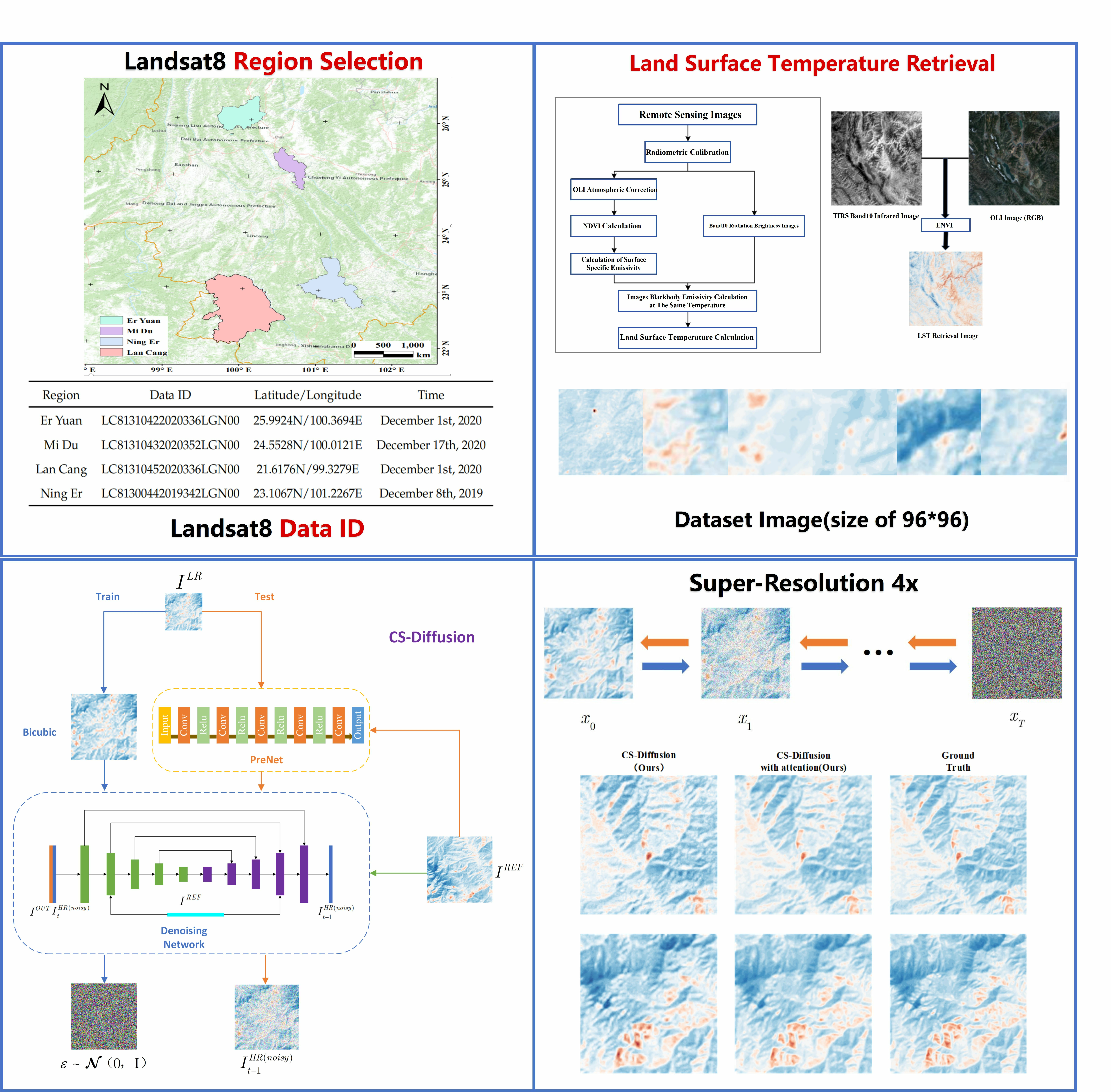
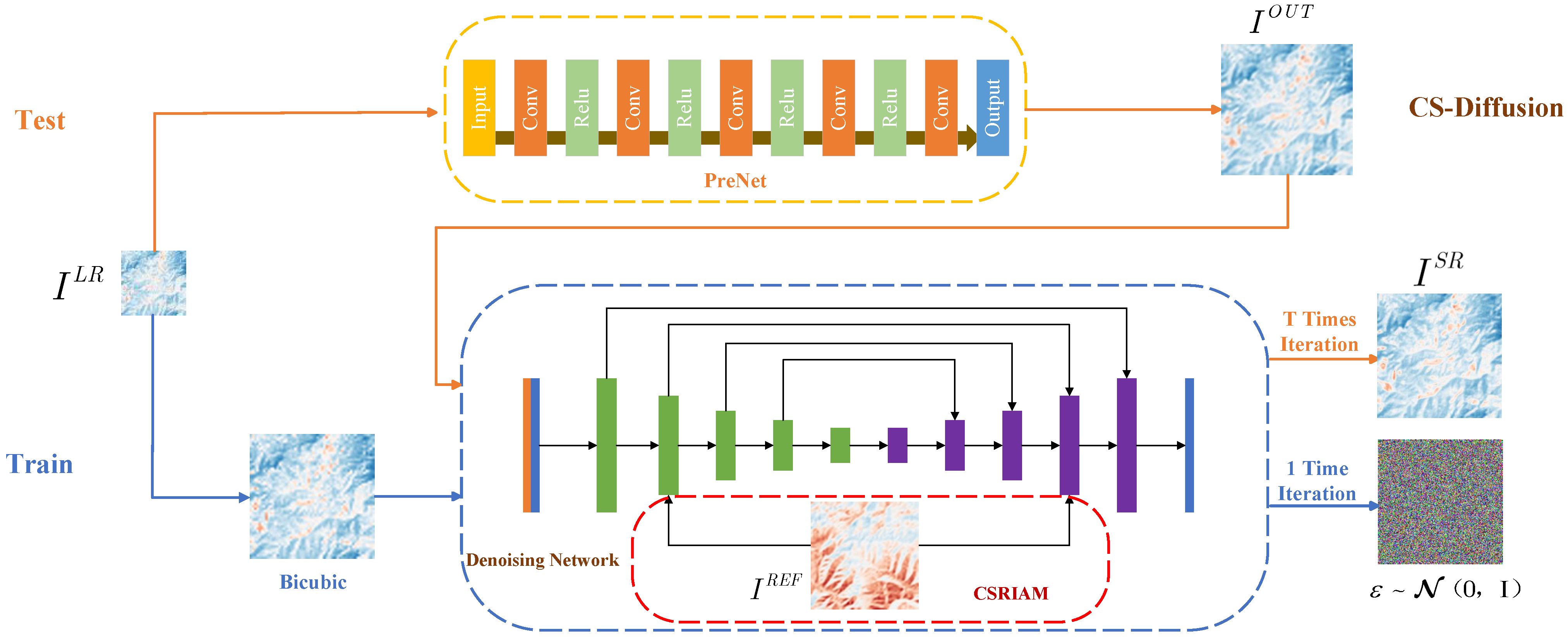
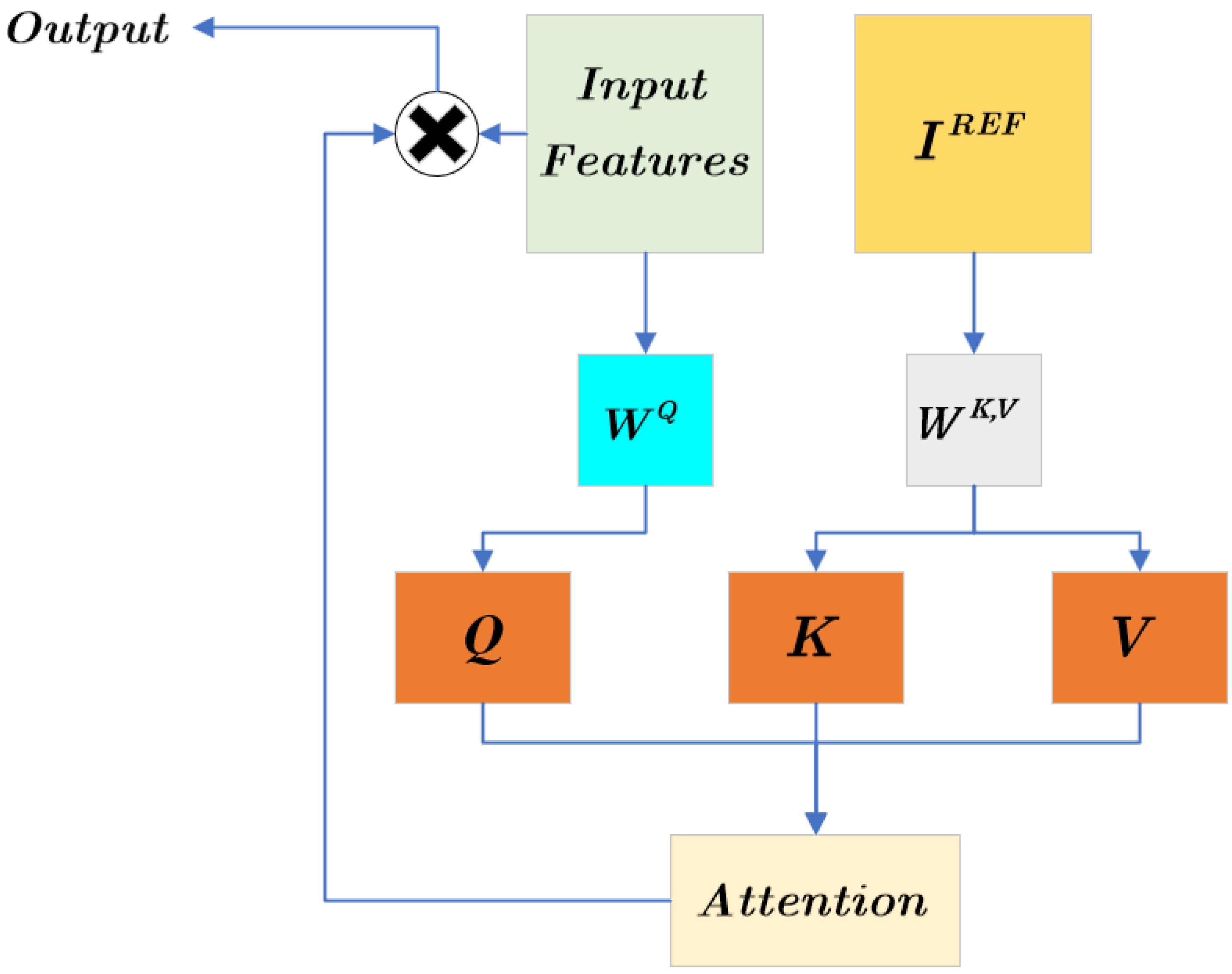
To address these issues, we proposed the Cross-Scale Diffusion (CS-Diffusion) method, which combines the advantages of super-resolution based on reference images and enables the network to learn features of reference images at different scales. Image super-resolution based on reference images can extract features from high-resolution reference images and be used to improve image quality. Our CS-Diffusion method introduces cross-scale reference images. First, due to the limitations of the Bicubic method itself, it is unable to perform good information recovery on low-resolution images. Therefore, we introduced Pre-Super-Resolution Net (PreNet), which can preliminarily restore the quality of the LR image. Based on the SR3 [22], we replaced its conditional input (Low-resolution image with Bicubic interpolation to target resolution) in the SR3 method with the output of our PreNet, whose inputs are low-resolution images; after that, we concatenated it with high-resolution images with noise. We used the same dataset to train PreNet to have the ability of pre-super-resolution. Finally, after the training of the diffusion model, we found that the super-resolution effect of LST retrieval images was greatly improved. Meanwhile, we proposed the Cross-Scale Reference Image Attention Mechanism, which could fuse the downsampled feature image and the high-resolution reference image, and reduce the information loss caused by the downsampling process. After the introduction of this mechanism, the noise of the super-resolution image was greatly reduced, and the recovery effect on geothermal anomaly points was greatly improved.

The main contributions of this article are as follows:

1. We proposed a network PreNet, which takes a low-resolution image as its input, and its output is used as the conditional input of the diffusion model. This method enhanced the effect of image reconstruction, resulting in an improvement in indices.

2. In response to the problem of information loss in U-Net downsampling, we proposed the Cross-Scale Reference Image Attention Mechanism to provide high-resolution reference features for the U-Net feature maps, greatly enhancing the information recovery ability of denoising networks.

In the next section, we introduce the proposed cross-scale diffusion method. PreNet is discussed in Section 2.1. The main structure of the denoising network is discussed in Section 2.2. The structure of the Cross-Scale Reference Image Attention Mechanism is discussed in Section 2.2.4.

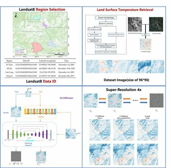
Figure 1 shows the overall framework of our CS-Diffusion method, using two types of logic for training and testing.

2. Methodology

2.1. Pre-Super-Resolution Network

2.1.1. The Structure of Pre-Super-Resolution Network

Our method aims to improve the super-resolution ability of the conditional diffusion model by improving the image quality of the conditional input of the diffusion model. We used PreNet to achieve the task of improving conditional input. The Pre-Super-Resolution Network (PreNet) takes the low-resolution image from Bicubic interpolation to the target resolution as the input, and outputs a pre-super-resolution image. Inspired by SRCNN [18] and VGG [32], we found that convolutional neural networks have strong performance in pre-reconstructing images. In addition, deep convolutional neural networks can extract features. Based on the above, we designed a PreNet as a convolutional neural network for image pre-reconstruction.

2.1.2. Loss Function

We take the Mean Squared Error (MSE) as the loss function of the PreNet network, and the $I^{OUT}$ is the output of PreNet:

$$I^{OUT}=P\left(I^{LR}\right),$$

(1)

where $P\left(\right)$ and $I^{OUT}$ represent the PreNet network and its output image. $I^{LR}$ represents the low-resolution image. The loss function used is MSE:

$$L^{Prenet}=\sum _{x=1}^W\sum _{y=1}^H{(I_{x,y}^{OUT}-I_{x,y}^{HR})}^2.$$

(2)

The meaning of $L^{Prenet}$ is to subtract the output of the network pixel by pixel from the original image and take its sum of squares. MSE is the most widely used optimization target in the field of image super-resolution [33], and many SOTA (State-Of-The-Art) methods use this loss function [34]. By optimizing the loss function, we can obtain a convolutional neural network, namely PreNet, which can pre-reconstruct images. Through this network, we can properly recover the information of low-resolution images with great information loss, to prepare for subsequent super-resolution work.

We found that PreNet can improve the quality of Bicubic interpolation images. Therefore, compared with the image using Bicubic interpolation directly for the target resolution, improving the quality of $I^{OUT}$ is simpler for the network. When training the denoising network, we still use the Bicubic interpolation image as the conditional input of our denoising network.

The training algorithm for PreNet is shown in Algorithm 1. We make the output of PreNet and $I^{HR}$ the MSE loss function and perform gradient descent so that the network can obtain the ability to recover the image quality initially.

Algorithm 1 Training PreNet

1: for: 2: $I^{OUT}=P\left(I^{LR}\right)$ 3: Take a gradient descent step on: ${\nabla }_{\theta }{\parallel P\left(I^{LR}\right)-I^{HR}\parallel }_2$ 4: until converged 5: end for

2.2. Cross-Scale Diffusion

2.2.1. Denoising Diffusion Probabilistic Models

The Denoising Diffusion Probabilistic Model (DDPM) [35] has achieved great success in fields such as data generation and medical image segmentation [36], and its performance also has great potential in the field of image super-resolution.

DDPM is divided into a forward process and backward process. For raw data, $x_0\sim q\left(x_0\right)$, which includes T diffusion processes. Each step adds Gaussian noise to the data $x_{t-1}$ in the previous step according to the following equation:

$$x_t=\sqrt{{\alpha }_t}{x}_{t-1}+\sqrt{1-{\alpha }_t}\epsilon ,$$

(3)

where ${\alpha }_t$ is a constant determined by t, and $\epsilon$ is Gaussian white noise with standard normal distribution satisfying $\epsilon \sim N(0,I)$.

The above equation can be equivalently expressed as:

$$q\left(x_t\right|x_{t-1})=N(x_t;\sqrt{1-{\beta }_t}{x}_{t-1},{\beta }_{t}I),$$

(4)

where ${\beta }_t$ is the variance used for each step, and ${\beta }_t\in (0,1)$, ${\beta }_t=1-{\alpha }_t$. Obviously, the diffusion process is a Markov process:

$$q\left(x_{1:T}\right|x_0)=\prod _{t=1}^{T}q\left(x_t\right|x_{t-1}).$$

(5)

The schematic diagram of the forward process and backward process is shown in Figure 2, where p represents the conditional probability distribution of the backward process, and q represents the conditional probability distribution of the forward diffusion process, which is known. Our goal is to train a network that can simulate p and use it to recover images from noise (i.e., backward process).

2.2.2. Conditional Diffusion Model

Inspired by SR3 [22], we use the conditional diffusion model for super-resolution of the conditional input, and we form an image pair $\left\{I_i^{LR},I_i^{HR\left(noisy\right)}\right\}$, where $I^{HR\left(noisy\right)}$ represents the HR image with noise, and its meaning is as follows:

$$I_t^{HR\left(noisy\right)}=\sqrt{{\sigma }_t}{I}^{HR}+\sqrt{1-{\sigma }_t}\epsilon ,$$

(6)

similar to ${\beta }_t$ in DDPM, ${\sigma }_t={\prod }_{t=1}^T{\alpha }_i$ is the variance of noise, and $\epsilon \sim N(0,I)$ is the noise of standard normal distribution. To train a denoising network $D_{\theta }$, we need to add noise to $I^{HR}$ according to the above equation. In order to train the network $D_{\theta }$, we use the following loss function:

$$Loss=\parallel D_{\theta }(I^{LR},\sqrt{{\sigma }_t}{I}_t^{HR}+\sqrt{1-{\sigma }_t}\epsilon ,I^{Ref},{\sigma }_t{)-\epsilon \parallel }_2,$$

(7)

where the input to the denoising network $D_{\theta }$ consists of the low-resolution image $I^{LR}$, the noised high-resolution image, the variance of the noise added, and the reference image. Our aim is to train a denoising network $D_{\theta }$ so that the output always remains Gaussian white noise $\epsilon \sim N(0,I)$ when the input changes. The training process of our denoising model is shown in Algorithm 2:

Algorithm 2 Training denoising network.

1: for: 2: $\sigma \sim p\left(\sigma \right)$ 3: $\epsilon \sim N(0,I)$ 4: Take a gradient descent step on: ${\nabla }_{\theta }\parallel D_{\theta }(I^{LR},\sqrt{{\sigma }_t}{I}_t^{HR}+\sqrt{1-{\sigma }_t}\epsilon ,I^{Ref},{\sigma }_t{)-\epsilon \parallel }_2$ 5: end for

For a batch of training data, we select a variance ${\sigma }_t$ related to iteration round t, and add noise to $I^{HR}$ for training in the form of affine transformation, i.e., Equation (6) according to this variance. We need to make the output of the denoising network $D_{\theta }$ approach $\epsilon \sim N(0,I)$ so that the noise can be completely separated from the noisy $I_t^{HR\left(noisy\right)}$. We perform a single iteration to denoise a batch of $I_t^{HR\left(noisy\right)}$ for each training session.

After we obtain the trained denoising network $D_{\theta }$, we can simulate the backward propagation conditional probability distribution of the Markov chain, which is related to the iteration round t. We discuss the network structure of $D_{\theta }$ in Section 2.2.3.

The denoising network $D_{\theta }$ can learn the distribution characteristics of the training data during the training process and then complete the image super-resolution reconstruction in the reverse process. In the reverse process, we obtain the output $\epsilon$ through the denoising network $D_{\theta }$ as shown in the following equation:

$$D_{\theta }(I^{LR},I_t^{HR\left(noisy\right)},I^{Ref},{\sigma }_t)=\epsilon ,$$

(8)

and the input of the denoising network includes low-resolution images $I^{LR}$, noisy high-resolution images $I_t^{HR\left(noisy\right)}$, reference images $I^{Ref}$, and noise variance ${\sigma }_t$.

The reverse process is a Markov process, so the probability distribution between adjacent iteration rounds has the following properties:

$$p_{\theta }\left(I_{0:T}^{HR\left(noisy\right)}\right|I^{LR})=p_{\theta }\left(I_T^{HR\left(noisy\right)}\right)\prod _{t=1}^{T}p\left(I_{t-1}^{HR\left(noisy\right)}\right|I_t^{HR\left(noisy\right)},I^{LR}),$$

(9)

where $I_{0:T}^{HR\left(noisy\right)}$ represents a noisy high-resolution image with any number of iterations, and during training, $I_T^{HR\left(noisy\right)}$ represents pure noise, which will form a conditional input with $I^{LR}$ to infer the number of adjacent iterations. In the process of testing, that is, the super-resolution process, as the number of iterations increases, the denoising network gradually recovers the noisy high-resolution image from the noise.

According to Equations (6) and (8), it can be inferred that:

$$I^{HR}=\frac{1}{\sqrt{{\sigma }_t}}(I_t^{HR\left(noisy\right)}-\sqrt{1-{\sigma }_t}{D}_{\theta }(I^{LR},I_t^{HR\left(noisy\right)},I^{Ref},{\sigma }_t)).$$

(10)

But we cannot directly obtain high-resolution image $I^{HR}$ using this equation because our denoising model $D_{\theta }$ can only solve the noise $\epsilon \sim N(0,I)$ of one iteration at a time. Therefore, when performing the super-resolution reconstruction of the reverse process, we need to perform a complete T-iterations reverse process.

For each iteration, we can deduce the equation of the reverse process of adjacent iteration rounds according to the Markov property, i.e., Equation (9):

$$I_{t-1}^{HR\left(noisy\right)}=\frac{1}{\sqrt{{\alpha }_t}}(I_t^{HR\left(noisy\right)}-\frac{1-{\alpha }_t}{\sqrt{1-{\sigma }_t}}{D}_{\theta }(I^{OUT},I_t^{HR\left(noisy\right)},I^{Ref},{\sigma }_t))+\sqrt{1-{\alpha }_t}\epsilon ,$$

(11)

when $t=0$, we can obtain the super-resolution reconstructed image $I^{SR}$. As shown in Equation (11), we replaced $I^{LR}$ with $I^{OUT}$ for the super-resolution.

The algorithm for super-resolution reconstruction is shown in Algorithm 3. We first sampled noise of the same resolution as the image from standard Gaussian noise and used it as a conditional input. After T iterations, $I^{HR}$ (with $I^{LR}$ as the probability distribution reference) was recovered step by step from the noise, which also means that we obtained the super-resolution image $I^{SR}$.

Algorithm 3 Super-resolution.

1: $I_T^{HR\left(noisy\right)}\sim N(0,I)$: 2: for $t=T:1$: 3: $\epsilon \sim N(0,I)$ if $t>1$, else $\epsilon =0$ 4: $I_{t-1}^{HR\left(noisy\right)}=$ $\frac{1}{\sqrt{{\alpha }_t}}(I_t^{HR\left(noisy\right)}-\frac{1-{\alpha }_t}{\sqrt{1-{\sigma }_t}}{D}_{\theta }(I^{OUT},I_t^{HR\left(noisy\right)},I^{Ref},{\sigma }_t))$ $+\sqrt{1-{\alpha }_t}\epsilon$   5: end for 6: return $I_0^{HR\left(noisy\right)}\left(I^{SR}\right)$

2.2.3. Structure of Denoising Network

We used U-Net [37] as the backbone of the denoising model, which can increase the feature space dimension of images. Because the conditional probability distribution of the reverse process is very complex, a large number of high-dimensional features are required. The U-Net structure we use is shown in Figure 3:

$D_{\theta }$ is based on the U-Net structure and is stimulated by ResNet [38]. The U-Net network introduces residual blocks, which can eliminate the problem of experimental degradation caused by deepening the network structure.

Each residual block of U-Net is represented by the Group Norm, Sigmoid, and Conv, after performing N residual blocks on the feature map, downsampling is performed, and so on.

For U-Net, although the feature maps were concatenated with the same dimensional upsampling feature maps before downsampling, the problem of downsampling information loss still exists. To address this issue, we introduced the Cross-Scale Reference Image Attention Mechanism in the denoising network, which reduces the impact of downsampling information loss and enhances the network’s ability to recover images. The denoising network structure is shown in Figure 3 when the attention mechanism size is set to half the target resolution.

The specific content of Cross-Scale Reference Image Attention Mechanism is discussed in Section 2.2.4.

2.2.4. Cross-Scale Reference Image Attention Mechanism

The purpose of super-resolution reconstruction work is to increase the information content of the image, and the U-Net network structure has a significant impact on the super-resolution reconstruction work due to the significant information loss during downsampling. In response to the information loss caused by downsampling, we creatively introduced a cross-scale reference image attention mechanism as shown in Figure 3: we used the downsampling feature map in U-Net as the query of the attention mechanism to query high-resolution reference images (feature maps), and used the reference image feature map as the key and value of the attention mechanism.

The Cross-Scale Reference Image Attention Mechanism can fuse the feature map information of high-resolution reference images into the corresponding dimension feature map of U-Net, introduce reference information into the network, and enable the denoising network $D_{\theta }$ to learn. The introduction of the attention mechanism of the cross-scale reference image reduces the impact of information loss caused by the downsampling of denoising network $D_{\theta }$, and makes the super-resolution reconstruction of the diffusion model work better.

As shown in Figure 4, Input_Features obtains a query matrix (as shown in Equation (12)) through the $W^Q$ network. The reference image is first dimensionally adjusted through $1\times 1$ convolution, and then the key and value matrices are obtained through the $W^{K,V}$ network (as shown in Equation (13)). Finally, the Q, K, and V matrices are used for attention mechanism calculations to obtain corresponding values (as shown in Equation (14)), which are then fed into the network.

$$Q=Con{v}_{W^Q}\left(Input\_Features\right),$$

(12)

by transforming the input features into dimensions and using them as a query matrix, preparations are made for the subsequent calculation of attention mechanisms:

$$K,V=Con{v}_{W^{K,V}}\left(Con{v}_{1\times 1}\left(I^{Ref}\right)\right),$$

(13)

we extracted the key and value matrices of the reference image features to obtain high-resolution reference image features and used them for attention value calculation with the query matrix, thereby enabling the attention mechanism part of the network to learn the ability to fuse high-resolution features:

$$Attention=Softmax(\frac{Q{K}^T}{\sqrt{Num\_Channels}})V,$$

(14)

where the final calculated attention value will be multiplied by the input features and integrated into the output features. In this way, we can reduce the impact of information loss caused by U-Net downsampling on super-resolution tasks.

Through experiments, it was found that after the introduction of the Cross-Scale Reference Image Attention Mechanism, the overall image quality and indicators of the reconstructed image were significantly improved.

3. Experimental Results and Discussions

3.1. Dataset Preparation

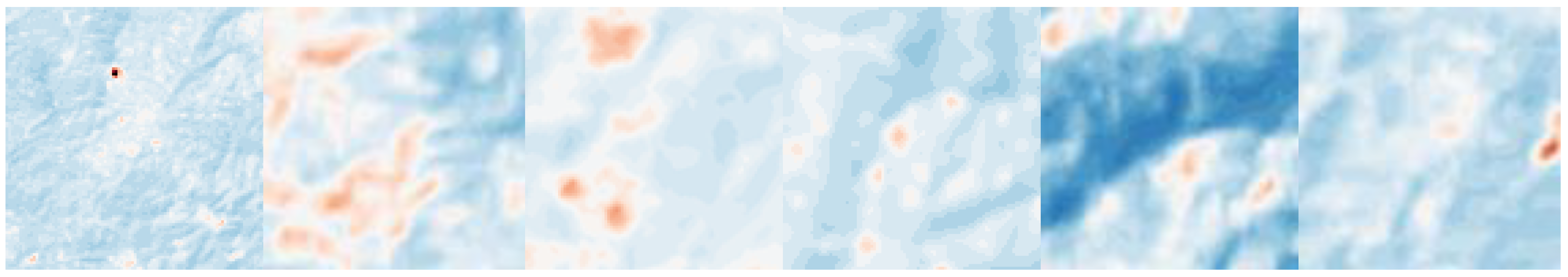
The commonly used image super-resolution datasets currently include COCO [39], CUFED5 [40], and ImageNet [41]. These datasets are composed of a large number of high-resolution images, which can be a good source of data for super-resolution tasks. However, for the super-resolution reconstruction task of LST images, the above datasets cannot effectively represent the characteristics of such images. Therefore, we used satellite remote sensing images to create SAT (Satellite And Temperature) datasets. In Figure 5, we present some images from the SAT dataset:

The data used in this article are all from the Landsat8 satellite. Its OLI land imager consists of 9 bands with a spatial resolution of 30 m. The thermal infrared sensor TIRS consists of two separate thermal infrared bands with a resolution of 100 m. The wavelength ranges of the two thermal infrared bands are Band10 (10.60∼11.19 $\mathsf{\mu }$m) and Band11 (11.50∼12.51 $\mathsf{\mu }$m). The thermal infrared band can record the amount of thermal radiation released from the ground and its diffusion range.

Table 1. Remote sensing image information.

Region	Data ID	Latitude/Longitude	Time
Er Yuan	LC81310422020336LGN00	25.9924N/100.3694E	1 December 2020
Mi Du	LC81310432020352LGN00	24.5528N/100.0121E	17 December 2020
Lan Cang	LC81310452020336LGN00	21.6176N/99.3279E	1 December 2020
Ning Er	LC81300442019342LGN00	23.1067N/101.2267E	8 December 2019

lists the specific information of the remote sensing image data we used, including region names, Data IDs, center longitude and latitude, and image capture times.

We used ENVI 5.3 to perform temperature retrieval on the original remote sensing images. Firstly, we used Landsat8 data for radiometric calibration. Then, we performed OLI (Operational Land Imager) atmospheric correction to eliminate the influence of atmospheric and lighting factors on ground reflection; NDVI (Normalized Difference Vegetation Index) calculation to detect vegetation growth status, vegetation coverage, and eliminate some radiation errors; and surface specific radiance calculation to obtain the temporal information of land surface. Finally, we calculated the blackbody radiance to obtain the land surface temperature image.

Our SAT dataset comes from four typical geothermal resource concentration areas in Eryuan, Midu, Lancang, and Ning’er, Yunnan Province, China, with a total of four high-resolution remote sensing images. The download path for images is http://www.gscloud.cn/. We selected satellite remote sensing images with cloud cover of less than $5\%$ for temperature retrieval, which can minimize the impact of weather factors on the experimental results. After retrieval of the land surface temperature using the ENVI platform, they were cut into 96 × 96 patches, including 14,976 $I^{HR}$ and 14,976 $I^{Ref}$. We used 182 sheets 224 × 224 patches as our test set to conduct comparative experimental tests on the performance of various models. Before sending the image into the network, we normalized it to facilitate network processing.

3.2. Training Details and Parameters Setting

The hardware platform we used is Intel Core i9-13900K + NVIDIA GeForce RTX 4090. The software platform is Python 3.10.11 + PyTorch 2.0.1 + CUDA 11.8 + CUDNN 8.2.1. The test indices for the comparative experiment are Peak Signal-to-Noise Ratio (PSNR), Structural Similarity (SSIM) [42], Learned Perceptual Image Patch Similarity (LPIPS) [43], and Frechet Inception Distance score (FID) [44], and the vision effects were taken as the reference indicator.

The formula for Peak Signal-to-Noise Ratio(PSNR) is as follows:

$$PSNR=20\times lo{g}_{10}(\frac{MA{X}_I}{\sqrt{MSE}}),$$

(15)

where $MA{X}_I$ is the maximum pixel value of the image, and MSE is defined as follows:

$$MSE=\frac{1}{H\times W}\sum _{x=0}^{W-1}\sum _{y=0}^{H-1}{[I(x,y)-T(x,y)]}^2,$$

(16)

where H and W represent the height and width of the image, $I(x,y)$ represents the pixel value of the test image, and $T(x,y)$ represents the pixel value of the target image.

Structural Similarity (SSIM) is an indicator that measures the similarity between two images and satisfies $SSIM\in [0,1]$, which is defined as follows:

$$SSIM(x,y)={\left[l(x,y)\right]}^{\alpha }{\left[c(x,y)\right]}^{\beta }{\left[s(x,y)\right]}^{\gamma },$$

(17)

$$l(x,y)=\frac{2{\mu }_x{\mu }_y+c_1}{{\mu }_x^2+{\mu }_y^2+c_2},$$

(18)

$$c(x,y)=\frac{2{\sigma }_{xy}+c_2}{{\sigma }_x^2+{\sigma }_y^2+c_2},$$

(19)

$$s(x,y)=\frac{{\sigma }_{xy}+c_3}{{\sigma }_x{\sigma }_y+c_3},$$

(20)

where $l(x,y)$ represents the comparison of image brightness, $c(x,y)$ represents the comparison of the image contrast, $s(x,y)$ represents the comparison of the image structure, $\mu$ represents the mean, $\sigma$ represents the standard deviation, ${\sigma }_{xy}$ represents the covariance, $c_1,c_2,c_3$ are constants, preventing the denominator from being 0, and $\alpha ,\beta ,\gamma$ are usually taken as 1.

The formula of Learned Perceptual Image Patch Similarity (LPIPS) is as follows:

$$LPIPS(x,y)=\sum _l\frac{1}{H_l{W}_l}\sum _{h,w}\left|\right|{\omega }_l\odot ({\widehat{x}}_{hw}^l-{\widehat{y}}_{0hw}^l){\left|\right|}_2,$$

(21)

where l means the layer of the feature map, ${\omega }_l$ means the neural network used to calculate the indicator, ${\widehat{x}}_{hw}^l$ means the pixels of SR, and ${\widehat{y}}_{0hw}^l$ means the pixels of HR.

The formula of the Frechet Inception Distance score (FID) is as follows:

$$FID(x,y)=\left|\right|{\mu }_x-{\mu }_y{\left|\right|}_2+Tr({\sigma }_x+{\sigma }_y-\sqrt{{\sigma }_x{\sigma }_y}),$$

(22)

where $Tr$ means the trace of the matrix.

We used 182 images for super-resolution testing on each model, with each image size of $224\times 224$. The corresponding low-resolution images were downsampled to different resolutions—$8\times$: $(28\times 28)$, $4\times$: $(56\times 56)$—and the average PSNR, SSIM, LPIPS, and FID were taken as the final indices for each model.

We selected the parameters according to the common diffusion model training details. In order to converge to the optimal network parameters, we set a lower learning rate and a higher training epochs, and the details of the experimental parameters are as follows.

The number of iterations of the diffusion model was set to T = 2000, and the size of the Cross-Scale Reference Image Attention Mechanism was set to 48 (training) and 112 (testing).

The number of residual blocks N corresponding to each feature of U-Net was set to 3, and the number of channels in U-Net was set to $[64,128,256,512,1024]$. The Batchsize was set to 16, we used the Adam optimizer, and the initial learning rate was 0.0001. The model converged after 600,000 iterations (300 epochs) of training on our dataset.

In addition, we also trained 300 epochs when training other models, and used the same dataset for training and testing. We selected Bicubic, SRCNN [18], SRGAN [19], ESRGAN [21], RCAN [45], HAT [46], and BebyGAN [47] as the comparative experimental models for SISR; TTSR [27] as the comparative experimental model based on reference image $I^{Ref}$; and SR3 [22], IDM [48], and SRDiff [49] as the diffusion-based comparative experimental models.

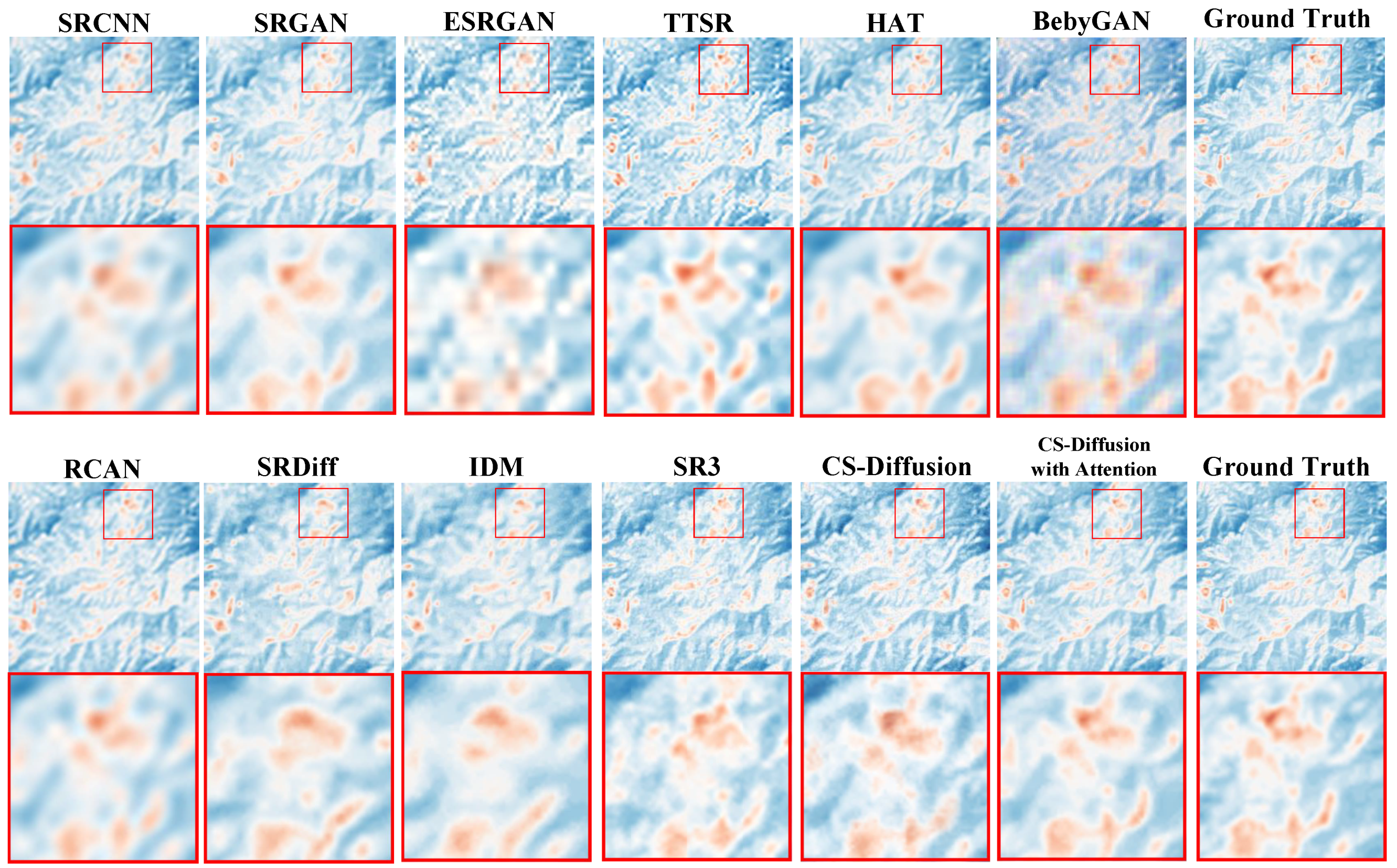
3.3. Benchmark Comparison and Ablation

We trained each model using the SAT dataset, performed 4× and 8× super-resolution, and tested the super-resolution visual effect of the model. The indices results of the comparative experiment are shown in

Table 2. Comparison of experimental indices: 4× and 8× super-resolution, where the best performance results are highlighted in bold font.

Scale	4×				8×
Method	PSNR↑	SSIM↑	LPIPS↓	FID↓	PSNR↑	SSIM↑	LPIPS↓	FID↓
Bicubic	30.45	0.8367	0.3104	122.56	27.29	0.6928	0.5091	159.83
SRCNN	32.02	0.8656	0.2865	87.35	27.68	0.7163	0.4723	132.34
SRGAN	30.07	0.8741	0.2168	47.71	26.55	0.7221	0.3027	50.88
ESRGAN	28.99	0.8138	0.3576	191.44	23.98	0.6862	0.5233	200.91
RCAN	32.60	0.8741	0.2575	79.51	26.89	0.7224	0.4587	121.91
HAT	29.04	0.8551	0.3271	103.97	25.04	0.8014	0.3637	178.57
BebyGAN	27.66	0.8411	0.2639	98.03	27.42	0.7353	0.3456	55.99
TTSR	29.08	0.8133	0.3009	103.79	×	×	×	×
SR3	30.34	0.8409	0.2385	39.87	27.15	0.6982	0.3019	53.26
IDM	30.93	0.8478	0.2196	44.32	27.28	0.6921	0.3327	51.29
SRDiff	30.59	0.8411	0.2055	45.98	26.11	0.7122	0.3429	67.32
CS-Diffusion	31.78	0.8707	0.2326	62.71	28.07	0.7371	0.2927	64.29
CS-Diffusion with Attention	33.02	0.8890	0.1696	44.86	28.33	0.7483	0.2731	52.28

, and the comparison of the experimental effects is shown in Figure 6. We found that although the model based on CNN can achieve higher PSNR and SSIM [42], and the model based on GAN [20] and Diffusion [35] can achieve higher LPIPS [43] and FID [44], it can be found from the experimental results in Figure 6 that high indices are not equivalent to excellent super-resolution visual effects, and the overall appearance of the image is also an important indicator. It can be observed that methods based on MSE optimization often lack high-frequency details of images, while methods based on generative adversarial networks are limited by interpolation methods, leading to block phenomena in images.

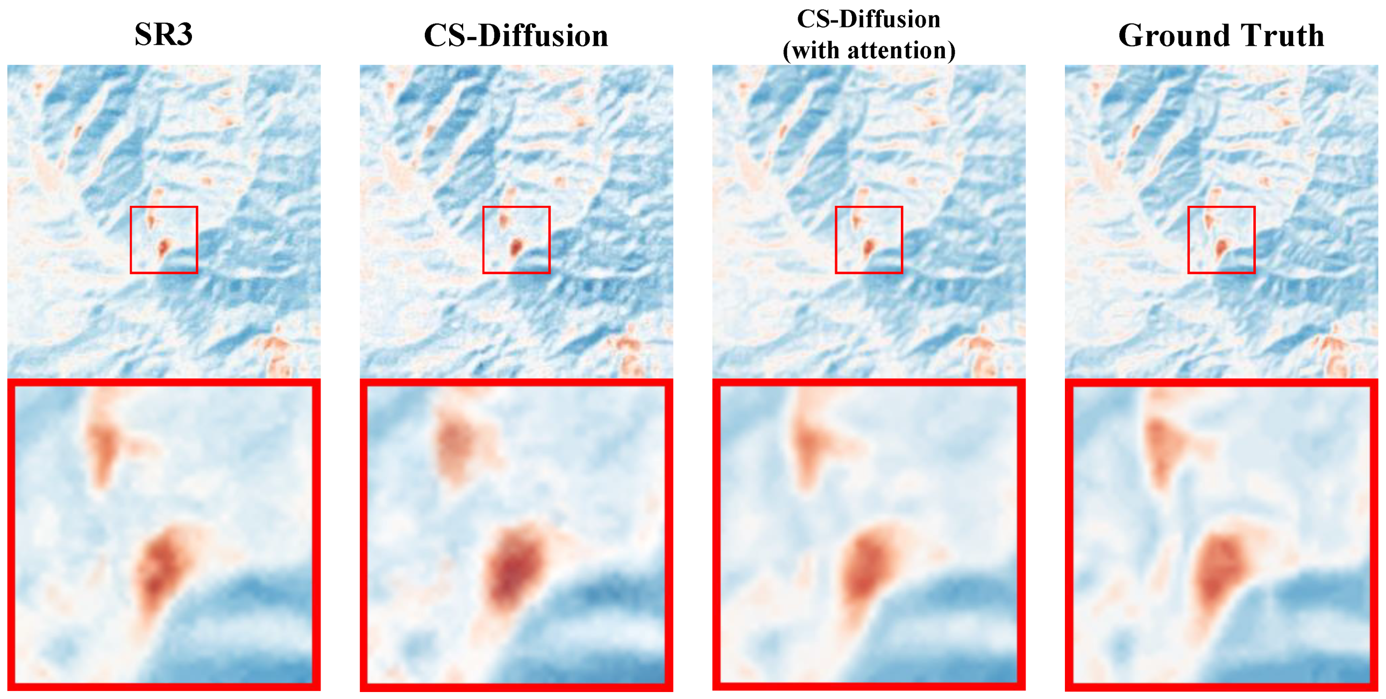
In the ablation experiment, we selected the SR3 [22] method as the baseline. According to the experimental comparison results, we demonstrated that introducing PreNet during testing can improve indices and visual effects compared to the SR3 method, which means our CS-Diffusion method (SR3 + PreNet) can greatly improve the super-resolution performance. The introduction of CSRIAM further improves the indices and eliminates the problem of white noise in the image. The specific visual effect can be seen in Figure 7.

In

Table 3. The ablation indices comparison: 4× super-resolution, where the best performance results are highlighted in bold font.

	Method	SR3	CS-Diffusion	CS-Diffusion (Attn)
Indices
PSNR↑		30.15	32.01	32.93
SSIM↑		0.8379	0.8716	0.8798
LPIPS↓		0.2412	0.2197	0.1685
FID↓		40.29	63.34	45.03

and Figure 7, we demonstrate the progress of our CS-Diffusion method based on the SR3 method. We found that the SR3 method will leave a portion of white noise on the reconstructed image, which is reflected in the form of white noise on the image. Although the addition of PreNet’s CS-Diffusion will, to some extent, solve this problem, there will still be some white noise present. After adding the Cross-Scale Reference Image Attention Mechanism, we effectively solved the problem of white noise on the image, resulting in an overall improvement in the quality of the reconstructed image and a more complete recovery of some geothermal anomalous areas.

According to the comparative test results, we found that our method can achieve the optimal effect in all comparison models on PSNR, SSIM and LPIPS, and can also be very close to the optimal performance on FID. Our method combines the advantages of reference-based super-resolution and diffusion models: excellent restoration of image quality, while reducing the excessive smoothing and over-sharpening of images. On this basis, noise removal in visual effects can be achieved (as shown in Figure 6).

3.4. Parameter Comparison Experiment

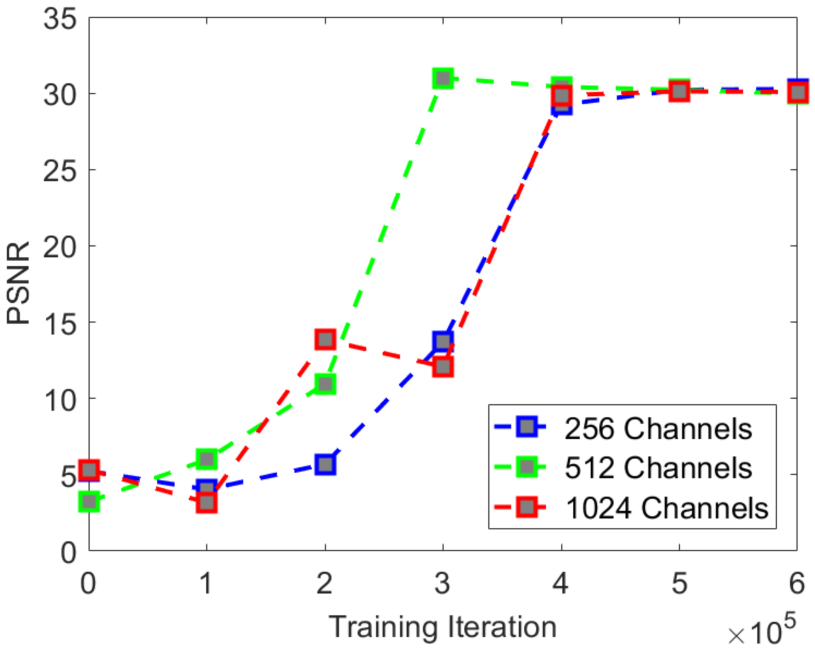
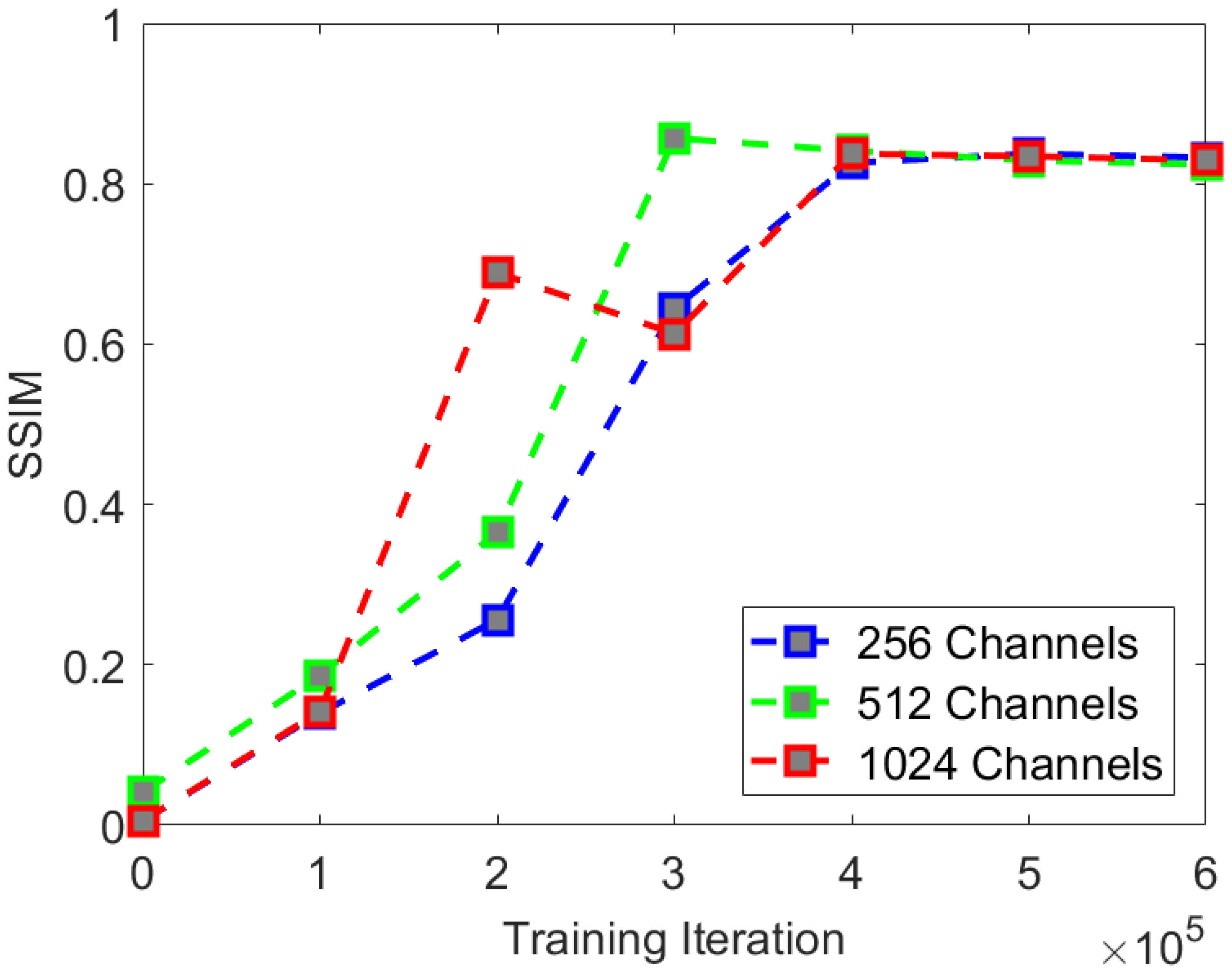
To explore the effects of network depth, number of iterations, and noise schedule on experimental results, we conducted multiple comparative experiments using the CS-Diffusion method. We found that the PSNR and SSIM can reflect whether the model converges. So we chose these two indices as the symbol of the rate of convergence. When conducting comparative experimental tests, our PSNR and SSIM were obtained by calculating the mean of the indices from the first three $224\times 224$ images in the test set.

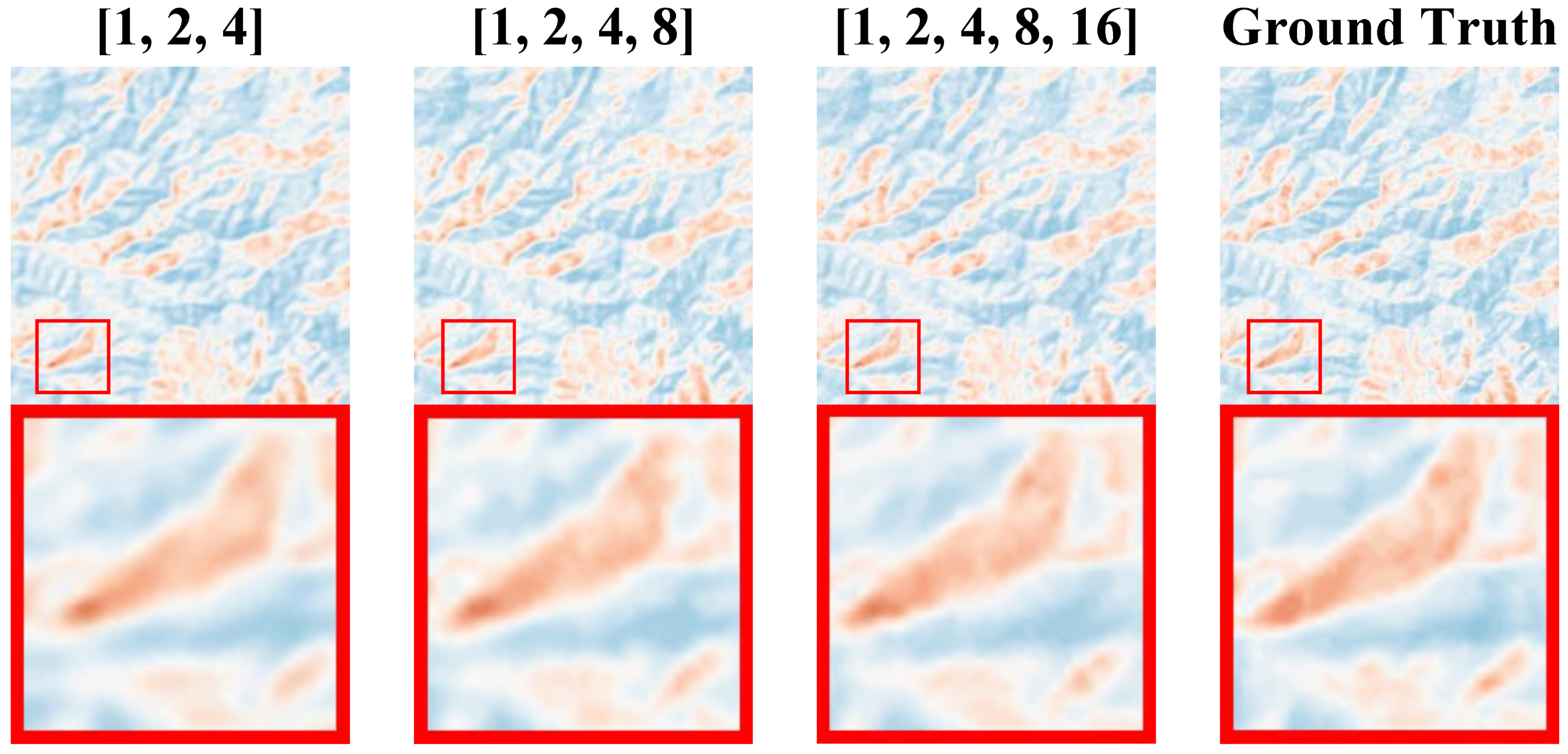
In the comparative experiment of network depth, we adopted three U-Net network depths: $[1,2,4],[1,2,4,8],[1,2,4,8,16]$. The comparative experimental indices are shown in

Table 4. Indices comparison of the depth of networks: 4× super-resolution, where the best performance results are highlighted in bold font.

	Depth	[1, 2, 4]	[1, 2, 4, 8]	[1, 2, 4, 8, 16]
Indices
PSNR↑		32.65	32.71	32.89
SSIM↑		0.8839	0.8850	0.8867
LPIPS↓		0.1889	0.1893	0.1732
FID↓		44.21	43.29	42.33

.

We found that with the increase in network depth, i.e., network parameters, there was a certain improvement in experimental indices. The network converges fastest at the depth of 512, but the optimal indices in the experiment are best at the depth of 1024. The rate of convergence of PSNR and SSIM is shown in Figure 8 and Figure 9. The comparison of visual effects is shown in Figure 10.

We found that when the network depth was [1, 2, 4, 8], the rate of convergence of the PSNR index was the fastest, and it could finally converge to an effect similar to the network depth [1, 2, 4, 8, 16]. It is difficult for the human eye to see the difference in the visual effect comparison. Therefore, when applying the CS-Diffusion model, we can sacrifice the metrics appropriately in exchange for training a model that is easier to converge and has smaller network parameters.

The rate of convergence of the SSIM index is similar to that of the PSNR index. Although we can improve the SSIM index with the increase in the network depth, there will not be much change in the visual effect. Therefore, we believe that the network depth of the CS-Diffusion model is the most cost-effective choice [1, 2, 4, 8].

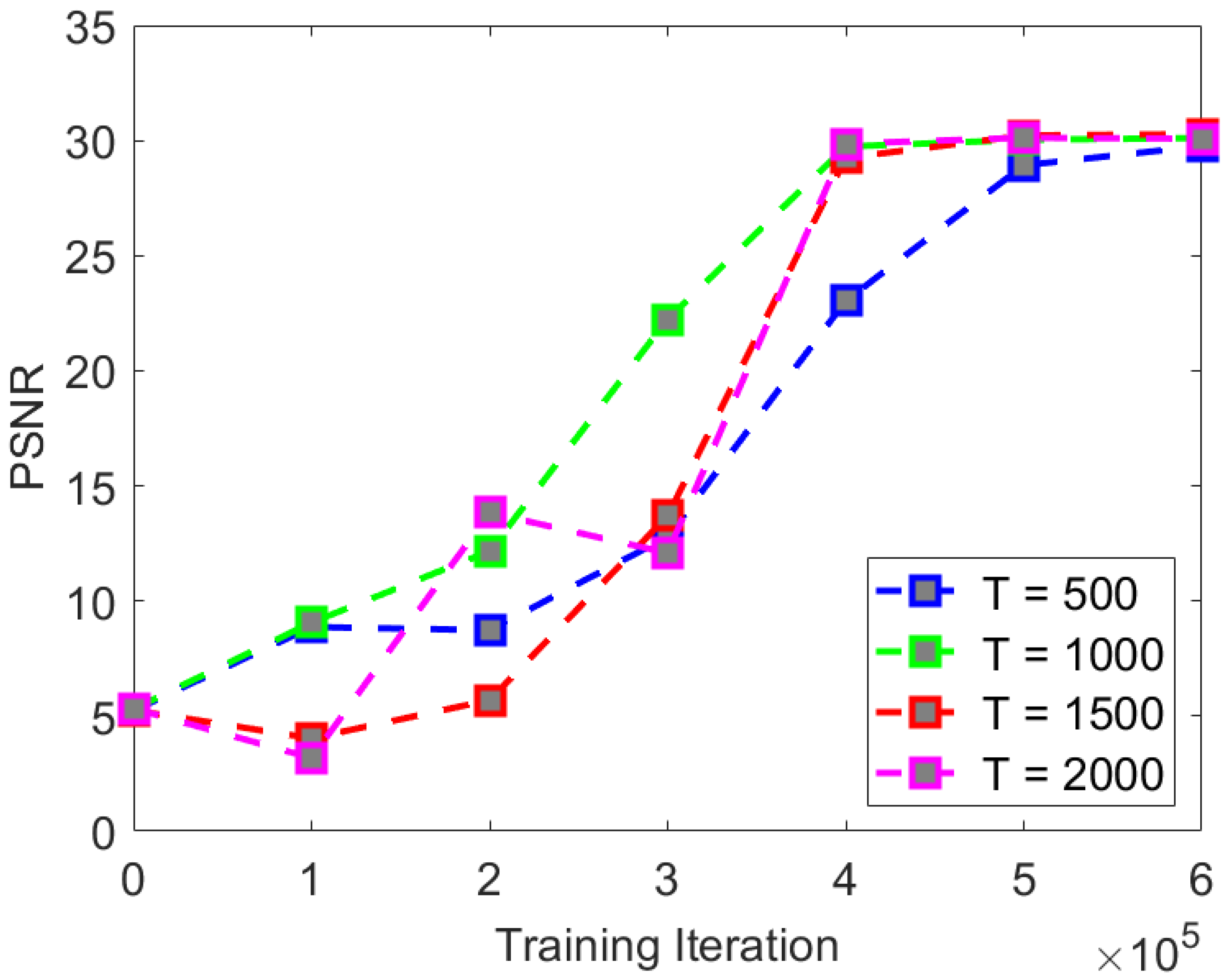
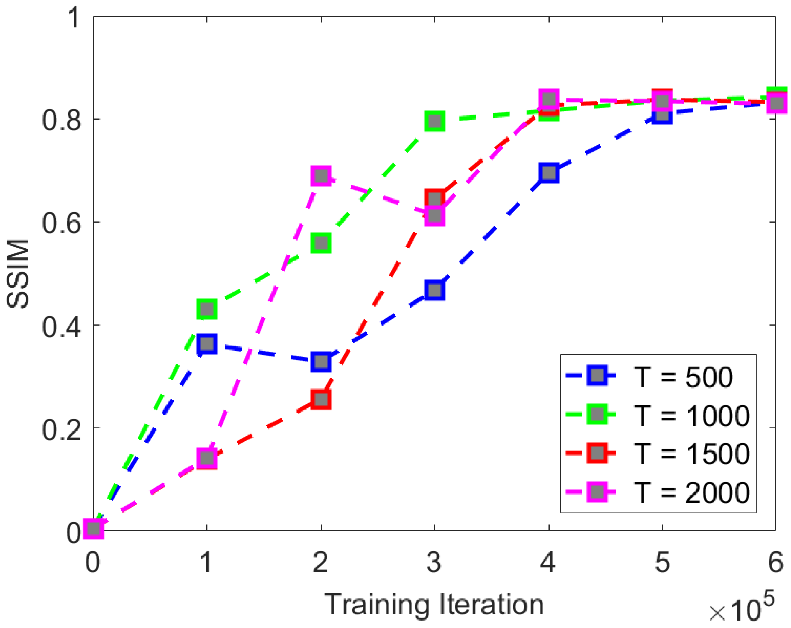
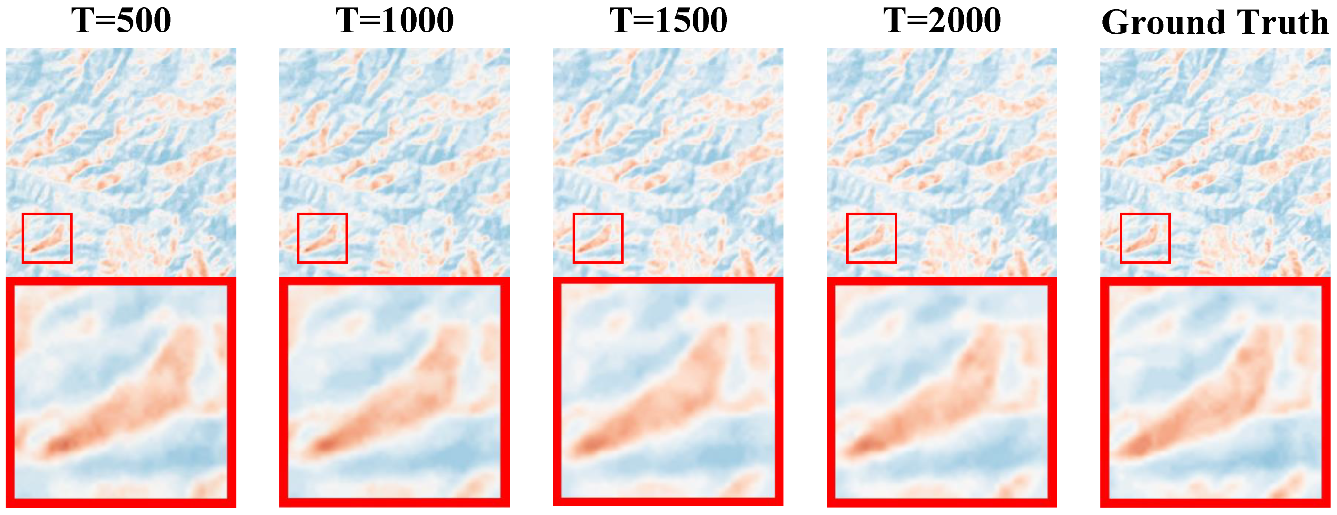
For the comparative experiment of iteration times, we adopted T = 500, 1000, 1500, and 2000 iteration times to compare the experimental indices and visual effects. The comparative experimental indices are shown in

Table 5. Indices comparison of iteration times: 4× super-resolution, where the best performance results are highlighted in bold font.

	Iteration	500	1000	1500	2000
Indices
PSNR↑		32.10	32.57	32.38	32.92
SSIM↑		0.8750	0.8824	0.8854	0.8878
LPIPS↓		0.2011	0.1929	0.1733	0.1678
FID↓		49.98	52.22	47.94	43.53

.

According to the experimental comparison, it can be seen that as the number of iterations increases, the experimental indices show a certain improvement. The rate of convergence of PSNR and SSIM is shown in Figure 11 and Figure 12. The comparison of the visual effects is shown in Figure 13. But as T grows, the time consumed by the testing process will increase significantly.

We found that when the number of iterations T is too small (i.e., T = 500), the PSNR and SSIM metrics cannot converge to good results. We believe that this is due to the small number of iterations, which leads to the inability to completely remove noise from the image. When the number of iterations is 1000, the rate of convergence and final convergence effect of both PSNR and SSIM indexes are better than those of other iterations. Therefore, we believe that T = 1000 is a good choice for the iteration number T of the CS-Diffusion method. As T increases as shown in Figure 13, the visual effect of the comparative experiment also improves, and the noise in the reconstructed image is reduced accordingly.

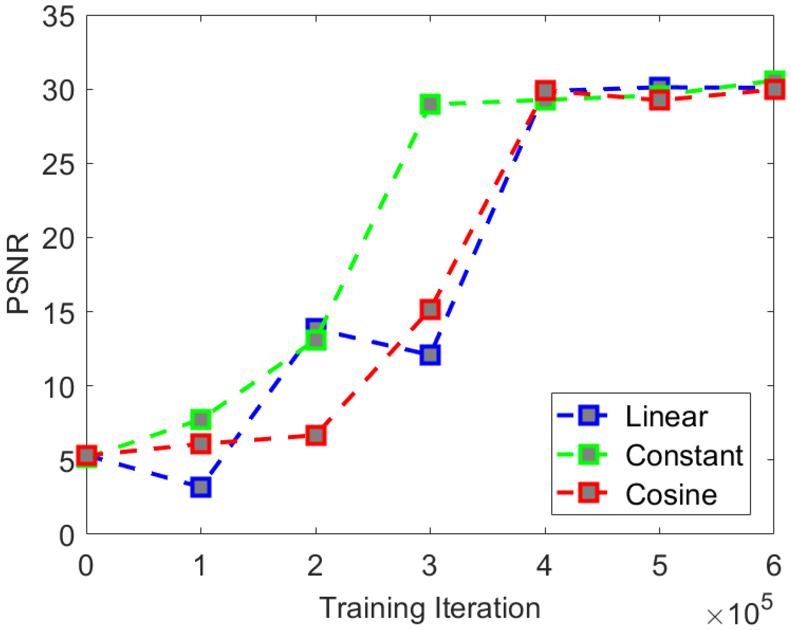
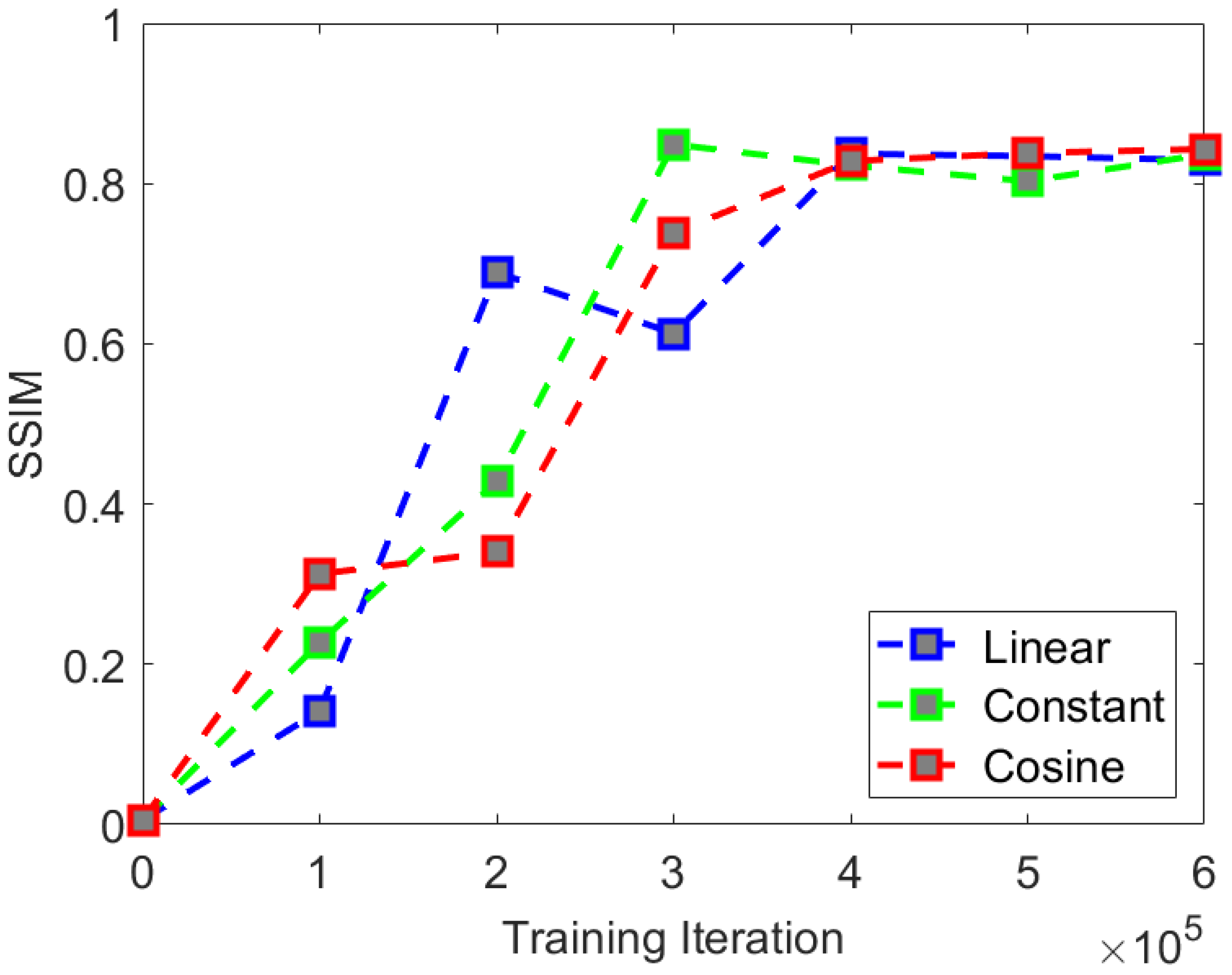
We selected three different noise schedules for comparative experiments. The relationship between linear variance ${\sigma }_t$ and iteration rounds t is as follows:

$${\sigma }_t={[\frac{Linear\_end-Linear\_start}{T}\times t]}_{t=1}^T,$$

(23)

where T is the number of iterations; $Linear\_start$ and $Linear\_end$ refer to the lower and upper bounds of ${\sigma }_t$; $Linear\_Start>0$; and $Linear\_end<1$.

The relationship between constant variance ${\sigma }_t$ and iteration round t is as follows:

$${\sigma }_t=C,$$

(24)

where C is a constant, and $C\in [0,1]$.

The relationship between cosine variance ${\sigma }_t$ and iteration number t is as follows:

$${\sigma }_t={[cos(\frac{T-t}{T+c}\times \frac{\pi }{2})]}_{t=1}^T,$$

(25)

where c is a constant and its function is to prevent the denominator from being 0, which can lead to calculation errors.

The comparative experimental indices are shown in

Table 6. Indices comparison of noise types: 4× super-resolution, where the best performance results are highlighted in bold font.

	Noise	Constant	Cosine	Linear
Indices
PSNR↑		32.67	32.57	32.38
SSIM↑		0.8838	0.8824	0.8854
LPIPS↓		0.1910	0.1713	0.1782
FID↓		47.01	55.79	44.28

.

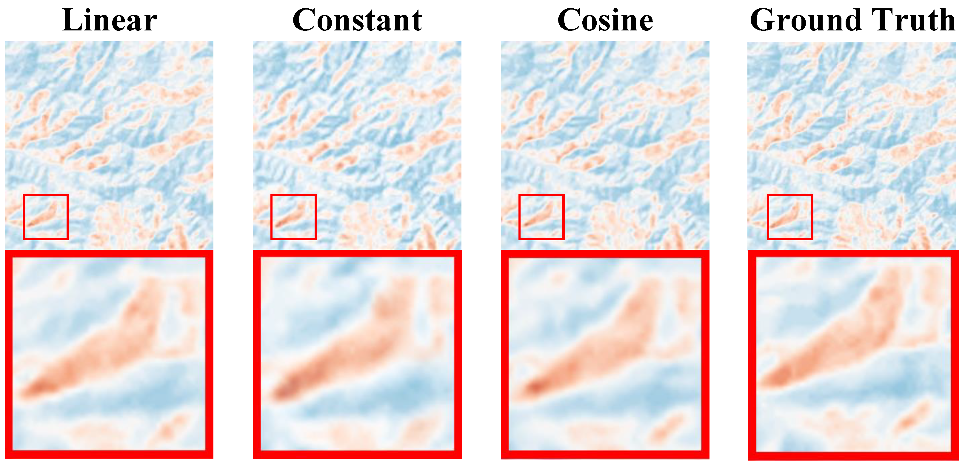
We found that in the comparative experiment, the three types of noise showed little difference in experimental indices. Although both experimental indices were not optimal under cosine noise, there was no significant difference in the visual effect compared to the other two types of noise. The rate of convergence of PSNR and SSIM are shown in Figure 14 and Figure 15. The comparison of visual effects is shown in Figure 16.

We found that in terms of the comparison of the rate of convergence of the experimental indices when using constant noise, the rate of convergence of the PSNR and SSIM indices is the fastest and can achieve a good final convergence effect. Therefore, we believe that the optimal noise selection for the CS-Diffusion method is constant noise.

Through comparative experiments on visual effects, we found that selecting the type of noise has little impact on the visual effects. Therefore, when training the CS-Diffusion model, we can give priority to the constant noise with a faster rate of convergence.

Through the above experiments, it can be found that we can adjust the experimental results by selecting different network parameters and the type of noise used during training. Different network parameters also have a significant impact on the super-resolution time. We also found that as the number of iterations T increases, the super-resolution effect improves. However, when T increases to a certain extent, the effect no longer shows a significant improvement but instead increases the time cost of super-resolution. At the same time, we found that as the depth of the network increases, the experimental effect will also improve but only within a certain range. Beyond this range, it will cause a sharp increase in the time cost of training and testing. In Section 3.5, a comparative experiment is conducted on the super-resolution time consumption between our model and other existing models.

3.5. Algorithm Time Consumption

Algorithms based on diffusion models are often time-consuming; this is due to the limitations of the diffusion model itself. In super-resolution tasks, the diffusion model needs to undergo T iterations to obtain SR images. Therefore, compared to the number of network parameters, the size of T is a direct factor affecting the algorithm’s time consumption. Our CS-Diffusion method can ensure the super-resolution effect while reducing T. Compared to SR3, we are able to reduce T to 300 without affecting the quality of SR images, greatly reducing the algorithm time consumption. We tested the time (in minutes) required for each model to perform 4× and 8× super-resolution on 182 images of size 224 × 224 in our test set. In

Table 7. Time consumption comparison of different models.

Time (min)↓	Method	SRCNN	SRGAN	RCAN	HAT	TTSR	SR3	IDM	SRDiff	CS-Diffusion (Attn)
Scale
4×		0.9	1.4	1.1	0.8	9.3	145.7	127.9	57.3	100.5
8×		0.9	1.9	1.3	0.9	×	135.4	121.9	69.1	100.9

, we show the time consumption of different models. We found that the models based on diffusion cost more time than the models based on CNN, but they can achieve better visual and indicator effects when dealing with time-insensitive super-resolution tasks, while methods based on diffusion models can achieve better results.

4. Conclusions

We proposed a CS-Diffusion model for the super-resolution of LST retrieval images. Different from single image super-resolution (SISR), this model can fuse the high-resolution features of the reference image, and use this part of the features for the super-resolution of low-resolution images. Among them, the Pre-Super-Resolution Network (PreNet) can improve the quality of Bicubic interpolation images. Through the optimization PreNet, we can obtain high-quality low-resolution images. This process improves the image quality of conditional input images of the diffusion model, thus improving the image quality of the final super-resolution images. The Cross-Scale Reference Image Attention Mechanism was proposed to address the issues of noise and geothermal anomaly recovery in super-resolution images. After introducing this mechanism, we successfully applied the texture features of high-resolution reference images to super-resolution tasks, and the indices and image quality of the super-resolution test were greatly improved. In Figure 17 we show more visual effects of the comparison experiment.

The model proposed in this article still has certain limitations, such as the slow speed of the image super-resolution reconstruction. This is because the denoising network we used uses a larger network width and has a higher dimension of feature space, which has significant limitations when dealing with time-sensitive super-resolution work. Meanwhile, the large number of parameters of the model is also a problem, as they require more computing power and occupy more resources during model training. And for the super-resolution of the large image, its occupied memory will increase exponentially. In subsequent work, the effect of super-resolution can be maintained while reducing the number of network parameters. Moreover, compared to deep learning-based methods, the convenience of traditional methods (such as no need for training, short time consumption, and low computational power requirements) is still irreplaceable.

In addition, further research can be conducted on the reconstruction of missing information in the image, optimizing the recovery of geothermal anomaly areas, and enhancing the generalization of the network structure.

References

1. Chiodi, A.; Tassi, F.; Báez, W.; Maffucci, R.; Invernizzi, C.; Giordano, G.; Corrado, S.; Bicocchi, G.; Vaselli, O.; Viramonte, J.G.; et al. New geochemical and isotopic insights to evaluate the geothermal resource of the hydrothermal system of Rosario de la Frontera (Salta, northern Argentina). J. Volcanol. Geotherm. Res. 2015, 295, 16–25. [Google Scholar] [CrossRef]
2. Quinao, J.J.; Zarrouk, S.J. Applications of experimental design and response surface method in probabilistic geothermal resource assessment–preliminary results. In Proceedings of the 39th Workshop on Geothermal Reservoir Engineering, Stanford, CA, USA, 24–26 February 2014. [Google Scholar]
3. Zaini, N.; Yanis, M.; Abdullah, F.; Van Der Meer, F.; Aufaristama, M. Exploring the geothermal potential of Peut Sagoe volcano using Landsat 8 OLI/TIRS images. Geothermics 2022, 105, 102499. [Google Scholar] [CrossRef]
4. Hou, J.; Huang, C.; Zhang, Y.; Guo, J. On the value of available MODIS and Landsat8 OLI image pairs for MODIS fractional snow cover mapping based on an artificial neural network. IEEE Trans. Geosci. Remote Sens. 2020, 58, 4319–4334. [Google Scholar] [CrossRef]
5. Liu, H.; Huang, B.; Zhan, Q.; Gao, S.; Li, R.; Fan, Z. The influence of urban form on surface urban heat island and its planning implications: Evidence from 1288 urban clusters in China. Sustain. Cities Soc. 2021, 71, 102987. [Google Scholar] [CrossRef]
6. Liu, H.; He, B.J.; Gao, S.; Zhan, Q.; Yang, C. Influence of non-urban reference delineation on trend estimate of surface urban heat island intensity: A comparison of seven methods. Remote Sens. Environ. 2023, 296, 113735. [Google Scholar] [CrossRef]
7. Guo, Y.; Deng, R.; Li, J.; Hua, Z.; Wang, J.; Zhang, R.; Liang, Y.; Tang, Y. Remote Sensing Retrieval of Total Nitrogen in the Pearl River Delta Based on Landsat8. Water 2022, 14, 3710. [Google Scholar] [CrossRef]
8. Habib, S.M.Z. Influence of Enhancing Urban Vegetation on Above-Ground Carbon Sequestration Dynamics in Arid Urban Lands: Case Study in Doha City, Qatar. Ph.D. Thesis, Hamad Bin Khalifa University, Ar-Rayyan, Qatar, 2021. [Google Scholar]
9. Gemitzi, A.; Dalampakis, P.; Falalakis, G. Detecting geothermal anomalies using Landsat 8 thermal infrared remotely sensed data. Int. J. Appl. Earth Obs. Geoinf. 2021, 96, 102283. [Google Scholar] [CrossRef]
10. Chou, C.; Park, J.; Chou, E. Generating high-resolution climate change projections using super-resolution convolutional LSTM neural networks. In Proceedings of the 2021 13th International Conference on Advanced Computational Intelligence (ICACI), Wanzhou, China, 14–16 May 2021; pp. 293–298. [Google Scholar]
11. Zhao, X.; Liu, K.; Gao, K.; Li, W. Hyperspectral time-series target detection based on spectral perception and spatial-temporal tensor decomposition. IEEE Trans. Geosci. Remote Sens. 2023, 61, 5520812. [Google Scholar] [CrossRef]
12. Zhao, X.; Li, W.; Zhao, C.; Tao, R. Hyperspectral target detection based on weighted cauchy distance graph and local adaptive collaborative representation. IEEE Trans. Geosci. Remote Sens. 2022, 60, 5527313. [Google Scholar] [CrossRef]
13. Yang, Q.; Yang, R.; Davis, J.; Nistér, D. Spatial-depth super resolution for range images. In Proceedings of the 2007 IEEE Conference on Computer Vision and Pattern Recognition, Minneapolis, MN, USA, 17–22 June 2007; pp. 1–8. [Google Scholar]
14. Zou, W.W.; Yuen, P.C. Very low resolution face recognition problem. IEEE Trans. Image Process. 2011, 21, 327–340. [Google Scholar] [CrossRef]
15. He, H.; Siu, W.C. Single image super-resolution using Gaussian process regression. In Proceedings of the CVPR 2011, Colorado Springs, CO, USA, 20–25 June 2011; pp. 449–456. [Google Scholar]
16. Schulter, S.; Leistner, C.; Bischof, H. Fast and accurate image upscaling with super-resolution forests. In Proceedings of the IEEE Conference on Computer Vision and Pattern Recognition, Boston, MA, USA, 7–12 June 2015; pp. 3791–3799. [Google Scholar]
17. Wang, Z.; Chen, J.; Hoi, S.C. Deep learning for image super-resolution: A survey. IEEE Trans. Pattern Anal. Mach. Intell. 2020, 43, 3365–3387. [Google Scholar] [CrossRef]
18. Dong, C.; Loy, C.C.; He, K.; Tang, X. Image super-resolution using deep convolutional networks. IEEE Trans. Pattern Anal. Mach. Intell. 2015, 38, 295–307. [Google Scholar] [CrossRef]
19. Ledig, C.; Theis, L.; Huszár, F.; Caballero, J.; Cunningham, A.; Acosta, A.; Aitken, A.; Tejani, A.; Totz, J.; Wang, Z.; et al. Photo-realistic single image super-resolution using a generative adversarial network. In Proceedings of the IEEE Conference on Computer Vision and Pattern Recognition, Honolulu, HI, USA, 21–26 July 2017; pp. 4681–4690. [Google Scholar]
20. Goodfellow, I.; Pouget-Abadie, J.; Mirza, M.; Xu, B.; Warde-Farley, D.; Ozair, S.; Courville, A.; Bengio, Y. Generative adversarial networks. Commun. ACM 2020, 63, 139–144. [Google Scholar] [CrossRef]
21. Wang, X.; Yu, K.; Wu, S.; Gu, J.; Liu, Y.; Dong, C.; Qiao, Y.; Change Loy, C. Esrgan: Enhanced super-resolution generative adversarial networks. In Proceedings of the European Conference on Computer Vision (ECCV) Workshops, Munich, Germany, 8–14 September 2018. [Google Scholar]
22. Saharia, C.; Ho, J.; Chan, W.; Salimans, T.; Fleet, D.J.; Norouzi, M. Image super-resolution via iterative refinement. IEEE Trans. Pattern Anal. Mach. Intell. 2022, 45, 4713–4726. [Google Scholar] [CrossRef]
23. Moser, B.B.; Shanbhag, A.S.; Raue, F.; Frolov, S.; Palacio, S.; Dengel, A. Diffusion Models, Image Super-Resolution and Everything: A Survey. arXiv 2024, arXiv:2401.00736. [Google Scholar]
24. Zhang, Y.; Zhang, L.; Song, R.; Tong, Q. A General Deep Learning Point–Surface Fusion Framework for RGB Image Super-Resolution. Remote Sens. 2023, 16, 139. [Google Scholar] [CrossRef]
25. Zhang, J.; Zheng, R.; Wan, Z.; Geng, R.; Wang, Y.; Yang, Y.; Zhang, X.; Li, Y. Hyperspectral Image Super-Resolution Based on Feature Diversity Extraction. Remote Sens. 2024, 16, 436. [Google Scholar] [CrossRef]
26. Zhang, Z.; Wang, Z.; Lin, Z.; Qi, H. Image super-resolution by neural texture transfer. In Proceedings of the IEEE/CVF Conference on Computer Vision and Pattern Recognition, Long Beach, CA, USA, 15–20 June 2019; pp. 7982–7991. [Google Scholar]
27. Yang, F.; Yang, H.; Fu, J.; Lu, H.; Guo, B. Learning texture transformer network for image super-resolution. In Proceedings of the IEEE/CVF Conference on Computer Vision and Pattern Recognition, Seattle, WA, USA, 13–19 June 2020; pp. 5791–5800. [Google Scholar]
28. Vaswani, A.; Shazeer, N.; Parmar, N.; Uszkoreit, J.; Jones, L.; Gomez, A.N.; Kaiser, Ł.; Polosukhin, I. Attention is all you need. In Proceedings of the Advances in Neural Information Processing Systems 30 (NIPS 2017), Long Beach, CA, USA, 4–9 December 2017. [Google Scholar]
29. Wang, P.; Zhang, H.; Zhou, F.; Jiang, Z. Unsupervised remote sensing image super-resolution using cycle CNN. In Proceedings of the IGARSS 2019—2019 IEEE International Geoscience and Remote Sensing Symposium, Yokohama, Japan, 28 July–2 August 2019; pp. 3117–3120. [Google Scholar]
30. Rabbi, J.; Ray, N.; Schubert, M.; Chowdhury, S.; Chao, D. Small-object detection in remote sensing images with end-to-end edge-enhanced GAN and object detector network. Remote Sens. 2020, 12, 1432. [Google Scholar] [CrossRef]
31. Nguyen, B.M.; Tian, G.; Vo, M.T.; Michel, A.; Corpetti, T.; Granero-Belinchon, C. Convolutional Neural Network Modelling for MODIS Land Surface Temperature Super-Resolution. In Proceedings of the 2022 30th European Signal Processing Conference (EUSIPCO), Belgrade, Serbia, 29 August–2 September 2022; pp. 1806–1810. [Google Scholar]
32. Simonyan, K.; Zisserman, A. Very deep convolutional networks for large-scale image recognition. arXiv 2014, arXiv:1409.1556. [Google Scholar]
33. Yang, C.Y.; Ma, C.; Yang, M.H. Single-image super-resolution: A benchmark. In Proceedings of the Computer Vision–ECCV 2014: 13th European Conference, Zurich, Switzerland, 6–12 September 2014; Proceedings, Part IV 13. Springer: Cham, Switzerland, 2014; pp. 372–386. [Google Scholar]
34. Shi, W.; Caballero, J.; Huszár, F.; Totz, J.; Aitken, A.P.; Bishop, R.; Rueckert, D.; Wang, Z. Real-time single image and video super-resolution using an efficient sub-pixel convolutional neural network. In Proceedings of the IEEE Conference On Computer Vision And Pattern Recognition, Las Vegas, NV, USA, 27–30 June 2016; pp. 1874–1883. [Google Scholar]
35. Ho, J.; Jain, A.; Abbeel, P. Denoising diffusion probabilistic models. Adv. Neural Inf. Process. Syst. 2020, 33, 6840–6851. [Google Scholar]
36. Wu, J.; Fang, H.; Zhang, Y.; Yang, Y.; Xu, Y. MedSegDiff: Medical Image Segmentation with Diffusion Probabilistic Model. arXiv 2022, arXiv:2211.00611. [Google Scholar]
37. Ronneberger, O.; Fischer, P.; Brox, T. U-net: Convolutional networks for biomedical image segmentation. In Proceedings of the Medical Image Computing and Computer-Assisted Intervention–MICCAI 2015: 18th International Conference, Munich, Germany, 5–9 October 2015; Proceedings, Part III 18. Springer: Cham, Switzerland, 2015; pp. 234–241. [Google Scholar]
38. He, K.; Zhang, X.; Ren, S.; Sun, J. Deep residual learning for image recognition. In Proceedings of the IEEE Conference on Computer Vision and Pattern Recognition, Las Vegas, NV, USA, 27–30 June 2016; pp. 770–778. [Google Scholar]
39. Carion, N.; Massa, F.; Synnaeve, G.; Usunier, N.; Kirillov, A.; Zagoruyko, S. End-to-end object detection with transformers. In Proceedings of the Computer Vision—ECCV 2020: 16th European Conference, Glasgow, UK, 23–28 August 2020; Proceedings, Part I 16. Springer: Cham, Switzerland, 2020; pp. 213–229. [Google Scholar]
40. Wang, Y.; Lin, Z.; Shen, X.; Mech, R.; Miller, G.; Cottrell, G.W. Event-specific image importance. In Proceedings of the IEEE Conference on Computer Vision and Pattern Recognition, Las Vegas, NV, USA, 27–30 June 2016; pp. 4810–4819. [Google Scholar]
41. Russakovsky, O.; Deng, J.; Su, H.; Krause, J.; Satheesh, S.; Ma, S.; Huang, Z.; Karpathy, A.; Khosla, A.; Bernstein, M.; et al. Imagenet large scale visual recognition challenge. Int. J. Comput. Vis. 2015, 115, 211–252. [Google Scholar] [CrossRef]
42. Wang, Z.; Bovik, A.C.; Sheikh, H.R.; Simoncelli, E.P. Image quality assessment: From error visibility to structural similarity. IEEE Trans. Image Process. 2004, 13, 600–612. [Google Scholar] [CrossRef]
43. Zhang, R.; Isola, P.; Efros, A.A.; Shechtman, E.; Wang, O. The unreasonable effectiveness of deep features as a perceptual metric. In Proceedings of the IEEE Conference on Computer Vision and Pattern Recognition, Salt Lake City, UT, USA, 18–23 June 2018; pp. 586–595. [Google Scholar]
44. Heusel, M.; Ramsauer, H.; Unterthiner, T.; Nessler, B.; Hochreiter, S. Gans trained by a two time-scale update rule converge to a local nash equilibrium. In Proceedings of the Advances in Neural Information Processing Systems 30 (NIPS 2017), Long Beach, CA, USA, 4–9 December 2017. [Google Scholar]
45. Zhang, Y.; Li, K.; Li, K.; Wang, L.; Zhong, B.; Fu, Y. Image super-resolution using very deep residual channel attention networks. In Proceedings of the European Conference on Computer Vision (ECCV), Munich, Germany, 8–14 September 2018; pp. 286–301. [Google Scholar]
46. Chen, X.; Wang, X.; Zhou, J.; Dong, C. Activating more pixels in image super-resolution transformer. arXiv 2022, arXiv:2205.04437. [Google Scholar]
47. Li, W.; Zhou, K.; Qi, L.; Lu, L.; Lu, J. Best-buddy gans for highly detailed image super-resolution. Proc. Aaai Conf. Artif. Intell. 2022, 36, 1412–1420. [Google Scholar] [CrossRef]
48. Gao, S.; Liu, X.; Zeng, B.; Xu, S.; Li, Y.; Luo, X.; Liu, J.; Zhen, X.; Zhang, B. Implicit diffusion models for continuous super-resolution. In Proceedings of the IEEE/CVF Conference on Computer Vision and Pattern Recognition, Vancouver, BC, Canada, 17–24 June 2023; pp. 10021–10030. [Google Scholar]
49. Li, H.; Yang, Y.; Chang, M.; Chen, S.; Feng, H.; Xu, Z.; Li, Q.; Chen, Y. Srdiff: Single image super-resolution with diffusion probabilistic models. Neurocomputing 2022, 479, 47–59. [Google Scholar] [CrossRef]
Figure 1. The structure of Cross-Scale Diffusion. When training, we use the bicubic method to interpolate low-resolution images to the target resolution as shown by the blue line. During testing, we use PreNet for pre-super-resolution of low-resolution images to the target resolution as shown by the orange line.
Remotesensing 16 01356 g001
Figure 2. Forward and reverse processes of diffusion, where x 0 is the original image, x T is the Gaussian white noise with standard normal distribution.
Remotesensing 16 01356 g002
Figure 3. The structure of the denoising network, where the depth of U-Net is (1, 2, 4, 8, 16).
Remotesensing 16 01356 g003
Figure 4. The structure of the Cross-Scale Reference Image Attention Mechanism, where Input Features is the feature maps obtained from U-Net downsampling, and I R E F is the feature maps obtained from the reference image through convolutional layers.
Remotesensing 16 01356 g004
Figure 5. Partial images in SAT dataset. This image shows the training set image, with a size of 96 × 96 .
Remotesensing 16 01356 g005
Figure 6. Comparison of experimental effects: 4× super-resolution. The selection of the red box on different images is the same, and we enlarged it to compare the visual details of the image.
Remotesensing 16 01356 g006
Figure 7. Comparison of model based on diffusion: 4× super-resolution. The selection of the red box on different images is the same, and we enlarged it to compare the visual details of the image.
Remotesensing 16 01356 g007
Figure 8. Rate of convergence of PSNR under different network depths.
Remotesensing 16 01356 g008
Figure 9. Rate of convergence of SSIM under different network depth.
Remotesensing 16 01356 g009
Figure 10. Comparison of visual effects of different network depths: 4× super-resolution. The selection of the red box on different images is the same, and we enlarged it to compare the visual details of the image.
Remotesensing 16 01356 g010
Figure 11. Rate of convergence of PSNR under different iterations.
Remotesensing 16 01356 g011
Figure 12. Rate of convergence of SSIM under different iterations.
Remotesensing 16 01356 g012
Figure 13. Comparison of visual effects of different iterations. 4× super-resolution. The selection of the red box on different images is the same, and we enlarged it to compare the visual details of the image.
Remotesensing 16 01356 g013
Figure 14. Rate of convergence of PSNR under different types of noise.
Remotesensing 16 01356 g014
Figure 15. Rate of convergence of SSIM under different types of noise.
Remotesensing 16 01356 g015
Figure 16. Comparison of visual effects of different noise: 4× Super-Resolution. The selection of the red box on different images is the same, and we enlarged it to compare the visual details of the image.
Remotesensing 16 01356 g016
Figure 17. Comparison of experimental effects: 4× super-resolution. The selection of the red box on different images is the same, and we enlarged it to compare the visual details of the image.
Remotesensing 16 01356 g017