Efficiently Refining Beampattern in FDA-MIMO Radar via Alternating Manifold Optimization for Maximizing Signal-to-Interference-Noise Ratio

Abstract

Joint transceiver beamforming is a fundamental and crucial research task in the field of signal processing. Despite extensive efforts made in recent years, the joint transceiver beamforming of frequency diverse array (FDA)-based multiple-input and multiple-output (MIMO) radar has received relatively less attention and is confronted with some tricky challenges, such as range–angle decoupling and the interaction between multiple performance metrics. In this paper, we initially derive the generalized ambiguity function of the FDA-MIMO radar to explore the intrinsic correlation between its waveform design and resolution. Following that, the joint beamforming optimization is formulated as a nonconvex bivariate quadratic programming problem (NBQP) with the aim of maximizing the Signal-to-Interference-Noise Ratio (SINR) of the FDA-MIMO radar system. Building upon this, we introduce an innovative alternating manifold optimization with nested iteration (AMO-NI) algorithm to address the NBQP. By incorporating manifold optimization into iterative updates of transmit waveform and receiving filter, the AMO-NI algorithm considers the interdependencies among the optimization variables. The algorithm efficiently and expeditiously finds global optimum solutions within a finite number of iterations. Compared with other methods, our approach yields a superior beampattern and higher SINR.

1. Introduction

As an emerging array structure, the FDA-MIMO radar has gained widespread attention over the past few years [1,2,3]. Due to its increased degrees of freedom (DOF) and range resolution capability, the FDA-MIMO radar has been widely applied to mainlobe interference suppression, target detection under clutter environment, and moving target tracking based on multidimensional information sources [4,5,6,7]. In the FDA-MIMO radar, orthogonal waveforms are emitted from the transmitter, and then the receiver is configured with a multi-matched filter to separate the signals [8,9]. Given this, the signals are synthesized into a time-independent and range–angle-dependent beampattern through the collection of signals from multiple channels [10]. The whole transceiver process is illustrated in Figure 1, which inherits the extra DOF from the frequency diversity of FDA radar and the flexibility from the waveform diversity of MIMO radar. One of the most critical problems in the process is to design the time-invariant equivalent transmit–receive waveforms with more concentrated energy, naturally giving rise to an important research topic—beamforming [11,12]. Beamforming aims to produce a multidimensional beampattern through the selection and configuration of transmit waveforms and receive filters, which is essential for improving target detection and localization and suppressing interference from complex scenarios [5,13,14,15]. In response to the topic, numerous researchers have dedicated substantial efforts.

Existing approaches are mainly divided into the following two categories. One is the widely adopted “two-step” method of beamforming, which involves the individual design of the transmitted waveform or the receive filters.

Specifically, a hybrid receive beamformer optimization for conventional MIMO radar under a framework of minimum variance distortionless response (MVDR) beamformer is proposed in [16], leveraging the idea of sparse signal recovery. In [17], an iterative scheme combined with MVDR is designed for the MIMO system with low probability of intercept (LPI) and multi-targets. Zhai et al. [18] designed a transmission waveform design method for MIMO radar through convex optimization, avoiding the relaxation of the objective function or constraints and improving computational efficiency. These methods are mainly developed for conventional radar systems and may not extend well to novel radar systems [19]. Under such circumstances, Mohammad et al. [20] designed a coordinate descent optimization framework for the coexisting system of communication and cognitive radar, achieving sequential optimization of efficient environmental sensing and radar transmit waveforms. The authors in [6] employed two-step independent optimization for the minimum redundancy FDA-MIMO radar, where the orthogonal subspace projection method is applied at the reception process and the covariance matrix is reconstructed at the transmission stage, achieving a beampattern with certain anti-interference capabilities. Despite this, the above design ignores the interrelationships between the variables, struggling in the optimality of the comprehensive performance of the system.

Another type of beamforming is the joint design of transmit waveform and receive filters, which is the mainstream at present [21,22,23]. This genre mainly uses an alternating optimization framework, which allows the multivariate problem to be decomposed into subproblems and solved cyclically [24]. The authors [25] addressed joint transceiver beamforming in MIMO radar by decomposing the optimization problem using a polynomial-time sequential convex approximation and norm constrained Capon beamformer (NCCB), achieving the injection of interference energy in each shared frequency band. Xu et al. [26] developed an alternating optimization algorithm based on semidefinite relaxation (SDR) to maximize radar mutual information. Those approaches [24,25,26] use convex relaxation and achieve better system performance in dealing with the problem of nonconvex functions and constraints. Recently, some researchers have extended this optimization framework to waveform design in the FDA-MIMO radar. In [27], the authors established an FDA antenna model with multiple overlapping subarrays and utilized ADMM to optimize the transmit beampattern, forming a beampattern with lower cross-correlation sidelobes. Gong et al. [28] proposed a primal–dual algorithm to enhance the LPI capability in the FDA-MIMO radar. To mitigate synthetic aperture radar interference, Lan et al. [29] developed iteration algorithms by introducing artificial interference, generating a trough-like transceiver beampattern with arbitrarily distributed broadened nulls.

In addition to the exploration of beamforming mentioned above, some researchers have explored and analyzed the impact of key parameters on radar system performance [19,30,31,32,33], providing theoretical foundations for waveform design. For example, Xiong et al. [19] derived the Cramér–Rao lower bound and mean square error for MUSIC-based range–angle estimation in the FDA-MIMO radar, while also setting thresholds for range and angle resolution in target detection and localization. In [30], the authors analyzed the ambiguity function characteristics of FDA radar and proposed a method for parameter optimization, leading to range-dependent beampatterns. The work of [31] establishes a closed-form model capable of generating a range–angle decoupled beampattern in FDA radar, and explores the relationship between FDA frequency increment and its beampattern. To further explore the potential applications of the FDA in target detection, radar imaging, and interference deception, the study by [32] extends the traditional ambiguity function to FDA radar and analyzes the resolution capabilities for target detection and imaging. Bang et al. [33] proposed a deceptive jamming method and the range-Doppler algorithm for a Synthetic Aperture Radar inspired by the paradigm of the FDA radar, showing promising results in high-resolution imaging.

While the aforementioned methods have achieved certain advances, there still remain the following challenges. (1) These methods primarily emphasize the waveform design for phased array or MIMO radars, and relatively few studies have taken into account the joint transceiver beamforming of the new radar system the FDA-MIMO radar, especially in improving the overall SINR of 2D beamforming. (2) The previous designs typically concentrate on solving the parameters of the transmitter and receiver using semidefinite and convex relaxation techniques, usually neglecting the decoupling of the two-dimensional beam during the optimization process. (3) To the best of our knowledge, there has been limited research analyzing the key parameters influencing 2D resolution in the waveform design of the FDA-MIMO radar. (4) Most optimization methods, when extended to FDA-MIMO, do not perform well in computational efficiency and resolution, as the optimization variable dimension in the FDA-MIMO radar is squared compared to conventional radar and the nonconvex objective function and constraints.

This paper introduces an effective beamforming method for joint transmission and reception in the FDA-MIMO radar as shown in Figure 2. Specifically, we first establish the signal model for the FDA-MIMO radar and derive its general ambiguity function to analyze the impact of parameters on range–angle resolution. In light of the analysis, we observe that the joint transceiver beamforming could alter the mainlobe width in the range–angle profile, and affect the range resolution and the coupling term. Upon this, a direct method is proposed for solving the SINR maximization problem under the constant modulus constraint, ingeniously avoiding convex relaxation. We simplify the optimization problem into a nonconvex binary quadratic programming problem (NBQP) and introduce a nested iterative alternating manifold optimization (AMO-NI) algorithm. In AMO-NI, transmit waveforms and receive filter weights are optimized alternately, reducing the coupling between variables and accelerating the convergence process. Simultaneously, AMO-NI transforms the feasible domain of the original problem from Euclidean space into a Riemannian manifold for computing the conjugate gradient descent direction and an effective step size under the Wolfe–Powell criterion, ensuring the algorithm’s convergence and obtaining a global optimal solution. The main contributions can be summarized as follows:

•

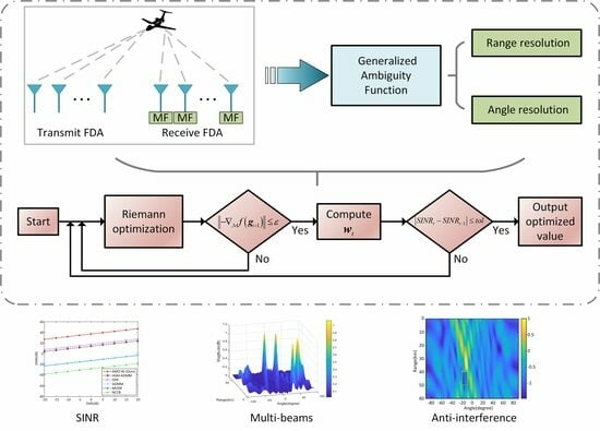
We derive the generalized ambiguity function of the FDA-MIMO radar for studying the key parameters that impact the range–angle resolution, and introduce a direct solution framework that avoids convex relaxation.

•

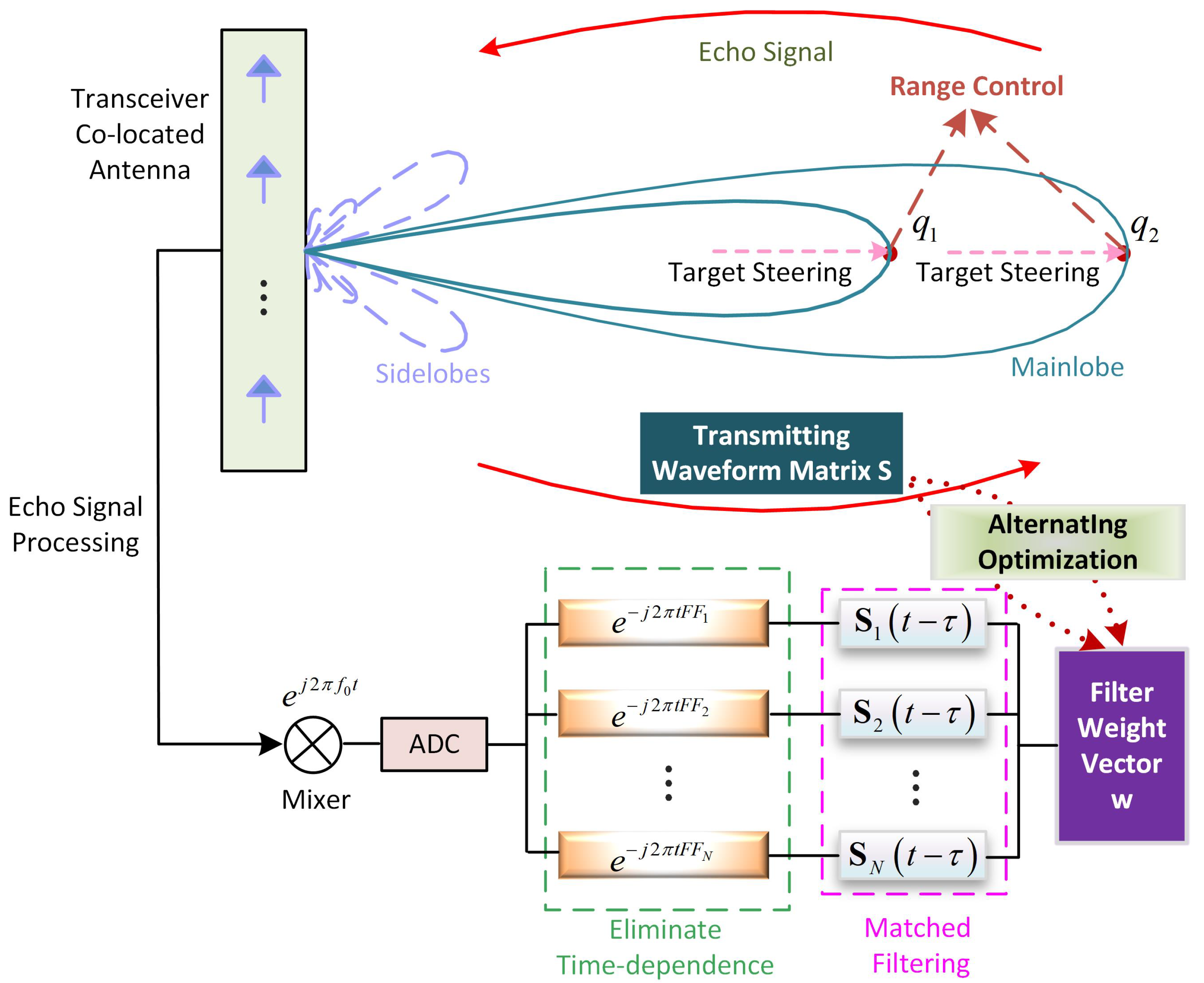
Under constant modulus conditions, the problem of jointly designing transmit waveforms and receive filter weights in the FDA-MIMO radar is transformed into a nonconvex bivariate quadratic programming problem (NBQP) for the simplicity of the subsequent solution.

•

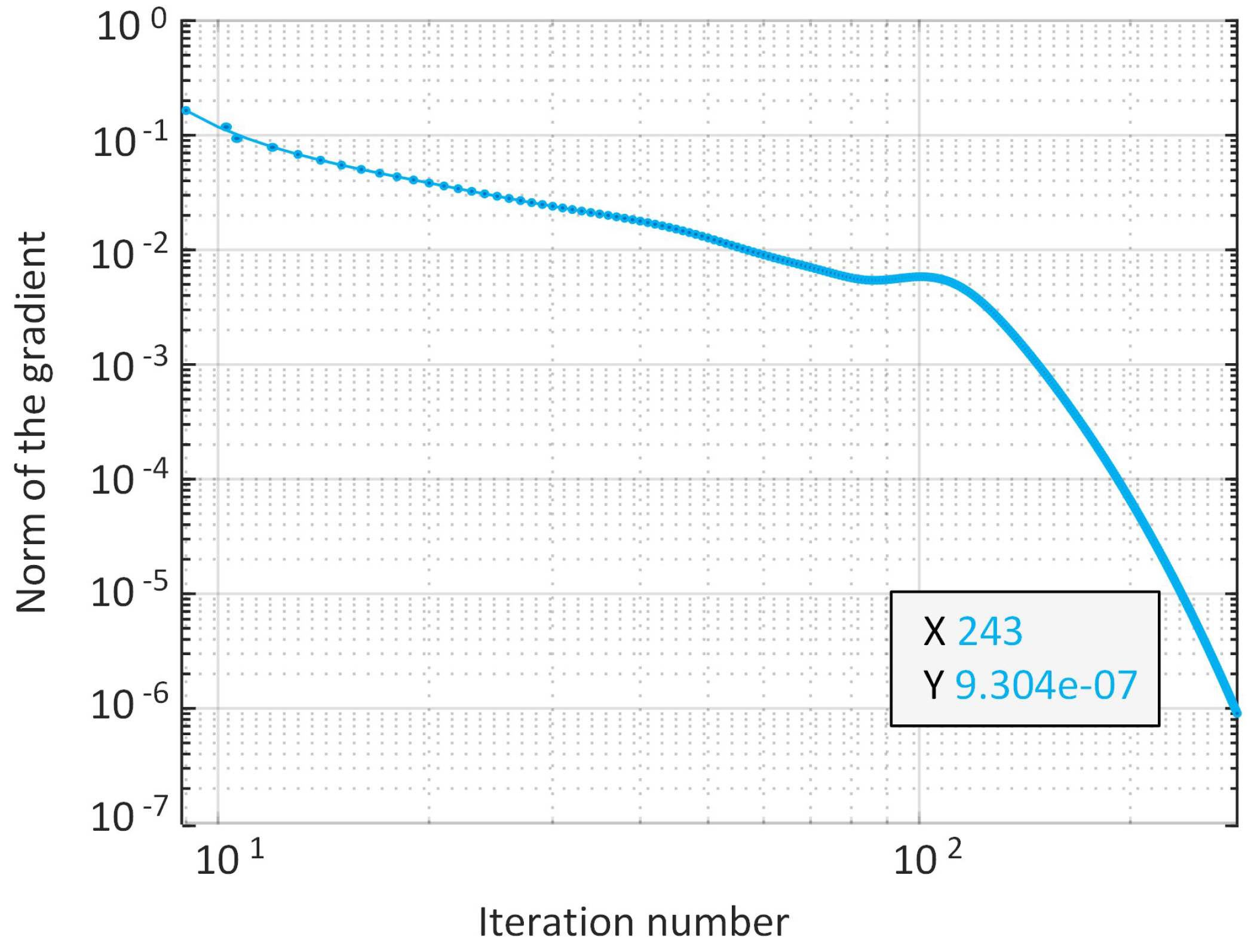
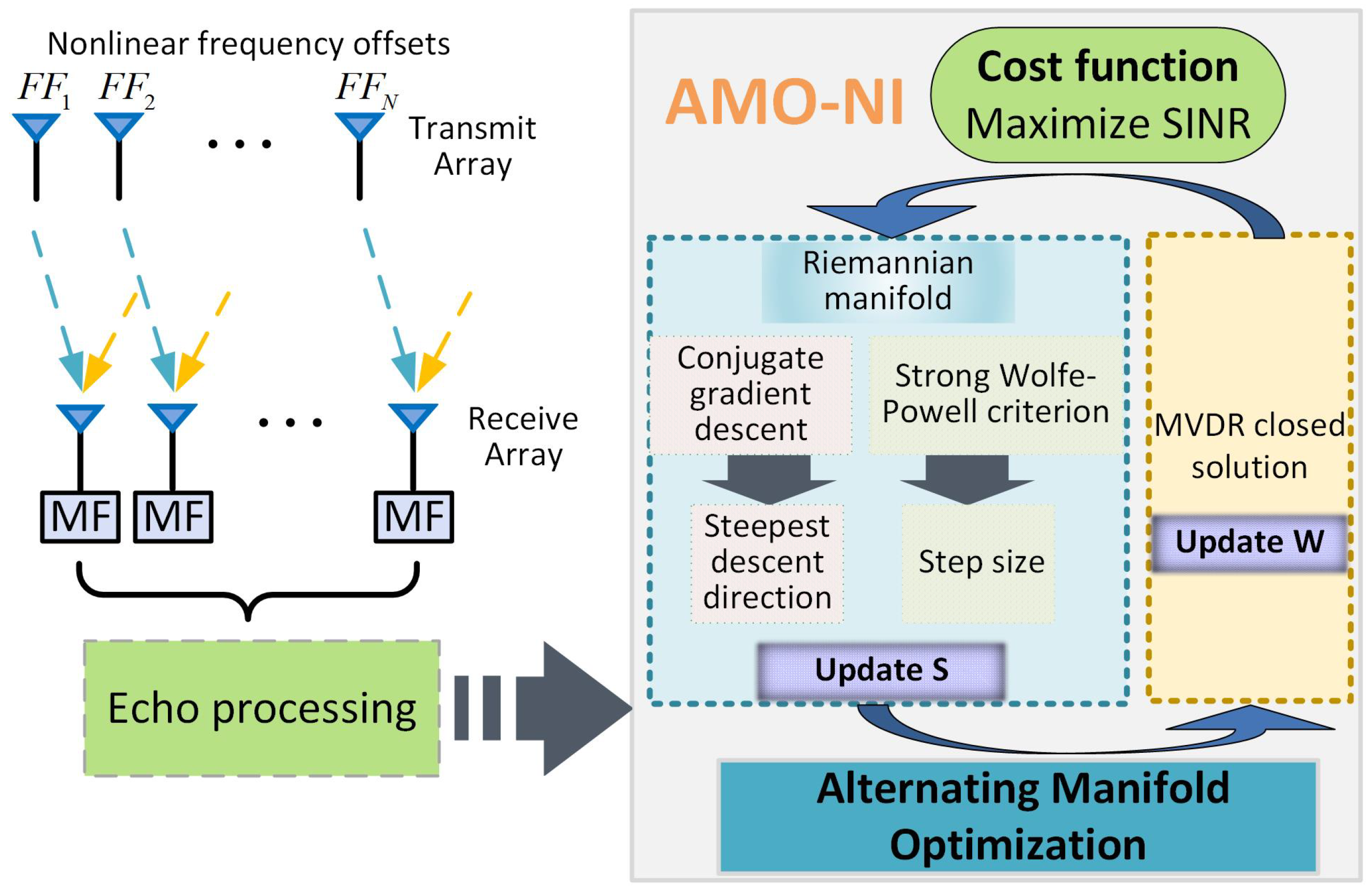
A nested iterative alternating manifold optimization (AMO-NI) algorithm is proposed for efficiently solving the NBQP and obtaining the optimal transmit waveforms and receive filter weights after a finite number of iterations.

•

Extensive experiments are conducted, and our method demonstrates a higher SINR while outperforming other methods in range–angle decoupling and computational efficiency.

The subsequent sections of this paper are structured as follows. Section 2 describes the signal model and ambiguity function of the FDA-MIMO radar and proposes the performance trade-off problem of optimizing the SINR and 2D beam resolution. In Section 3, we illustrate the alternating manifold optimization that maximizes the system SINR and maintains the decoupling of the transceiver beampattern in the range–angle dimension. Numerical simulations are conducted in Section 4 to verify the performance of our method in range–angle 2D beam and system SINR. Finally, Section 5 concludes the paper.

Notations: Boldface, bold italic, and italic letters are matrices, vectors, and variables. ${\mathbf{X}}^H$, ${\mathbf{X}}^T$, and ${\mathbf{X}}^{*}$ denote the conjugate transpose, transpose, and conjugate of the matrix $\mathbf{X}$. $\left|·\right|$ is the modulus of the complex scalar. ${\mathbf{I}}_N$ represents the N-dimensional identity matrix. ${\mathbb{C}}^N$ is an N-dimensional complex-valued vector space. $\Re \left(·\right)$ means the real part of a complex-valued number. ⊗, ⊙, and ⊘ are the Kronecker product, Hadamard product, and element-wise division.

2. Problem Formulation and Analysis

In this section, we first present the signal transmission model of the FDA-MIMO radar and derive the generalized ambiguity function for investigating the main factors that affect the range–angle resolution. Next, an optimization problem involving the transmitting waveform matrix and receiving filter weight vectors is formulated to improve SINR without sacrificing the range–angle resolution. Finally, we analyze the difficulties associated with the problem.

2.1. Signal Model

We consider a narrow-band colocated FDA-MIMO radar with N transmit antennas and M receive antennas. The transmit and receive antennas are uniform linear arrays with an inter-element spacing of d, where d equals half the wavelength. The $n-$th transmit signal is expressed as

$$x_n\left(t\right)=s_n\left(t\right)e^{j2\pi t\left(f_c+F{F}_n\right)},$$

(1)

where $s_n$ and $f_c$ represent the baseband waveform and carrier frequency. The frequency component $F{F}_n$ equals $\mathrm{Taylor}\left(n\right)\Delta fN(n-1)/2$, where $\mathrm{Taylor}\left(n\right)$ denotes the Taylor window function. We refer readers to [34,35,36] for more details. For the convenience of discussion, we assume a far-field point target located at azimuth angle ${\theta }_q$ and range $r_q$ without considering interference and noise. The received signal of the FDA-MIMO radar from the $m-$th element is defined as

$$\begin{array}{cc}\hfill y_m(t-\tau )& =\sum _{n=1}^N{x}_n(t-{\tau }_{n,m})\hfill \\ \hfill & \approx \zeta \sum _{n=1}^N{s}_n(t-\tau ){\mathrm{e}}^{j2\pi \left(f_c+F{F}_n\right)(t-{\tau }_{n,m})}\hfill \\ \hfill & =\zeta e^{j2\pi f_c\left[(t-\tau )+(m-1)\frac{d\sin \theta }{c}\right]}·\sum _{n=1}^N{s}_n(t-\tau )e^{j2\pi \left[(t-\tau )F{F}_n+f_c(n-1)\frac{d\sin \theta }{c}\right]},\hfill \end{array}$$

(2)

where ${\tau }_{n,m}=\left(2r-d\left[\left(n-1\right)+\left(m-1\right)\right]sin\theta \right)/\phantom{\left(2r-d\left[\left(n-1\right)+\left(m-1\right)\right]sin\theta \right)c}c$ represents the physical delay, and $2r$ denotes the distance between the first transmitting and receiving elements, while $\tau =2r/c$ is the reference element delay. $f_c$ and c are the carrier frequency and the speed of light. $\zeta$ is the complex amplitude, which undergoes channel transmission, target reflection, and amplitude attenuation.

As seen in Figure 1, the echo signals are separated via a multi-channel matching filter, where the term $e^{-j2\pi tF{F}_n}$ is employed to eliminate the time-dependence of the beampattern [37,38,39]. The $k-$th transmit code of $n-$th antenna is $s_n\left(k\right)$, where $n=1,2,...,N$ and $k=1,2,...,K$. K is the snapshot number of each pulse. The $k-$th waveform vector of N transmit antennas is represented as $\mathit{s}\left(k\right)={\left[s_1\left(k\right),s_2\left(k\right),...,s_N\left(k\right)\right]}^T\in {\mathbb{C}}^{N\times 1}$. For illustrative convenience, we define the transmit waveform matrix as $\mathbf{X}=\left[\mathit{s}\left(1\right),\mathit{s}\left(2\right),...,\mathit{s}\left(K\right)\right]\in {\mathbb{C}}^{N\times K}$. Stacking K snapshots, the transmission matrix can be integrated as $\mathbf{S}={\mathbf{X}}^T\otimes {\mathbf{I}}_M$. In general, the echo signal becomes more complicated under the presence of uncorrelated point-like interferences and Gaussian white noise. For clarity, the received signal $\mathit{y}$ stacked by the signals after multi-matched filters can be written as

$$\mathbf{y}=\sum _{q=1}^Q{\xi }_q\mathbf{S}{\mathbf{A}}_q+\sum _{l=1}^L{\varpi }_l\mathbf{S}{\mathbf{B}}_l+\mathbf{E},$$

(3)

where ${\xi }_q=\zeta e^{-j2\pi F{F}_n\tau }$ and ${\varpi }_l$ are the complex equivalent coefficient of the $q-$th target and the $l-$th interference source, and $l=1,2,\dots ,L$ (L indicates the number of interference sources). Here, ${\mathit{A}}_q=\mathit{u}\left(r_q,{\theta }_q\right)\otimes \mathit{v}\left({\theta }_q\right)$ and ${\mathit{B}}_l=\mathit{u}\left(r_l,{\theta }_l\right)\otimes \mathit{v}\left({\theta }_l\right)$ are the “virtual array” steering vectors. $\mathit{E}$ represents additional white Gaussian noise, instantiated as a random variable with a mean of zero and a variance of ${\sigma }^2$. The transmit steering vector $\mathit{u}\left(r_q,{\theta }_q\right)\in {\mathbb{C}}^{N\times 1}$, which effectively controls the range and angle of the transmitting beam, and the receive steering vector $\mathit{v}\left({\theta }_q\right)\in {\mathbb{C}}^{M\times 1}$ is defined as follows:

$$\begin{array}{cc}\hfill \mathit{u}\left(r_q,{\theta }_q\right)& ={\left[e^{j2\pi F{F}_1\frac{r_q}{c}},e^{-j4\pi F{F}_2\frac{r_q}{c}},\dots ,e^{-j4\pi F{F}_N\frac{r_q}{c}}\right]}^T\hfill \\ \hfill & \odot {\left[1,e^{j2\pi f_{c}d\frac{sin{\theta }_q}{c}},\dots ,e^{j2\pi f_c\left(N-1\right)d\frac{sin{\theta }_q}{c}}\right]}^T,\hfill \end{array}$$

(4)

$$\mathit{v}\left({\theta }_q\right)={\left[1,e^{-j2\pi f_{c}d\frac{sin{\theta }_q}{c}},\dots ,e^{-j2\pi f_{c}d\left(M-1\right)\frac{sin{\theta }_q}{c}}\right]}^T.$$

(5)

2.2. Generalized Ambiguity Function for FDA-MIMO Radar

Inspired by [30,32,40], we derive the generalized ambiguity function of the FDA-MIMO radar in joint transceiver beamforming for investigating the parameters that affect the range–angle resolution. We assume that the radial velocity of the target is depicted by the vector $\upsilon$ and utilize the parameter $\theta$ and $f_d$ to represent the position $\left(r,\theta \right)$ and Doppler shift of the target. With these definitions, the received signal ${y^{\prime }}_m$ after the spread spectrum is written as:

$$\begin{array}{cc}\hfill {y^{\prime }}_m\left(t-\tau \left(t;\Theta \right)\right)& =\zeta \left(t;\Theta \right)e^{j2\pi f_c\left[\left(t-\tau \left(t;\Theta \right)\right)+(m-1)\frac{d\sin {\theta }_q}{c}\right]}\hfill \\ \hfill & ·\sum _{n=1}^N{s}_n\left(t-\tau \left(t;\Theta \right)\right)e^{j2\pi \left[\left(t-\tau \left(t;\Theta \right)\right)F{F}_n+f_c(n-1)\frac{d\sin {\theta }_q}{c}\right]},\hfill \end{array}$$

(6)

where $\tau \left(t;\Theta \right)$ is a function related to the reference delay $\tau$. Time delays caused by inter-element spacing, electromagnetic wave propagation and target motivation are provided as follows:

$$\begin{array}{cc}\hfill \tau \left(t;\Theta \right)=& \tau \left(r\right)+{\tau }_{n,t}\left(\theta \right)+{\tau }_{m,r}\left(\theta \right)+{\tau }_d\left(\upsilon t\right)\hfill \\ \hfill =& 2r/\phantom{2\mathrm{R}c}c-ndsin\left(\theta \right)/\phantom{ndsin\left(\theta \right)c}c-mdsin\left(\theta \right)/\phantom{mdsin\left(\theta \right)c}c-2\upsilon t/\phantom{2\upsilon tc}c.\hfill \end{array}$$

(7)

In general, under the far-field target condition, we can ignore the inter-element spacing and the envelope delay. When $s_n\left(t-\tau \left(t;\Theta \right)\right)=s_n\left(t-\tau \right)$, the spread spectrum signal in (6) is simplified to

$$\begin{array}{cc}\hfill {y^{\prime }}_m\left(t-\tau \right)& =\zeta e^{j2\pi f_c\left[\left(t-\tau \right)+(m-1)\frac{d\sin {\theta }_q}{c}\right]}\hfill \\ \hfill & ·\sum _{n=1}^N{s}_n\left(t-\tau \right)e^{j2\pi \left[\left(t-\tau \right)F{F}_n+f_c(n-1)\frac{d\sin {\theta }_q}{c}\right]}\hfill \\ \hfill & ·e^{-j2\pi F{F}_n\left({\tau }_{n,t}\left(\theta \right)+{\tau }_{m,r}\left(\theta \right)\right)}{e}^{-j2\pi F{F}_n{\tau }_d\left(\upsilon t\right)},\hfill \end{array}$$

(8)

Here, only waveform design is emphasized without considering the propagation path loss. The complex amplitude of received signal is set to 1 in this context. Subsequently, down-conversion and matched filtering are used to separate signals, and M receiving signals are stacked. The term $e^{j2\pi \left(t-\tau \right)F{F}_n}$ is reshaped as a matrix $C\left(t-2r/\phantom{2rc}c\right)$. Here are some approximations, including $e^{-j2\pi F{F}_n{\tau }_d\left(\upsilon t\right)}=e^{j2\pi {\eta }_n{f}_{d}t}$, ${\eta }_n=F{F}_n/\phantom{F{F}_n{f}_c}{f}_c$ and $f_d=2\upsilon f_c/\phantom{2\upsilon f_{c}c}c$. The spread spectrum signal is rewritten as

$$\begin{array}{cc}\hfill \mathbf{J}\left(t;\Theta \right)& =e^{j2\pi t{f}_d}{\left[\mathit{u}\left(r,\theta \right)\otimes \mathit{v}\left(\theta \right)\right]}^T{\mathbf{S}}^T\left(t-2r/\phantom{2rc}c\right)C\left(t-2r/\phantom{2rc}c\right),\hfill \end{array}$$

(9)

where $f_d=\left(2\upsilon /\phantom{2\upsilon c}c\right)f_c$ represents the Doppler frequency, $\mathbf{S}\left(t\right)$ denotes the transmitting waveform matrix, and $C\left(t\right)=\left[e^{j2\pi tF{F}_1},e^{j2\pi tF{F}_2},...,e^{j2\pi tF{F}_N}\right]\otimes {\mathbf{I}}_k$ is the frequency offset delay (assuming $N=M$). We define the ambiguity function $\chi$ of the FDA-MIMO in joint beamforming as

$$\chi \left({\Theta }_1,{\Theta }_2\right)={\int }_{-\infty }^{\infty }\mathbf{J}\left(t,{\Theta }_1\right){\mathbf{J}}^{*}\left(t,{\Theta }_2\right)dt,$$

(10)

where ${\Theta }_1=\left\{r_1,{\theta }_1,f_{d1}\right\}$ and ${\Theta }_2=\left\{r_2,{\theta }_2,f_{d2}\right\}$. Furthermore, substituting $\mathbf{J}\left(t;\Theta \right)$ from (9) into (10), the ambiguity function ${\chi }_{FF}$ is redefined as Equation (11):

$$\begin{array}{c}\hfill \begin{array}{cc}\hfill {\chi }_{FF}\left({\Theta }_1,{\Theta }_2\right)& ={\int }_{-\infty }^{\infty }{e}^{j2\pi t{f}_d}\left[u\left(r,\theta \right)\otimes v\left(\theta \right)\right]\mathbf{S}\left(t-2r/\phantom{2rc}c\right)C\left(t-2r/\phantom{2rc}c\right)\hfill \\ \hfill & ·C^H\left(t-2r/\phantom{2rc}c\right){\mathbf{S}}^H\left(t-2r/\phantom{2rc}c\right){\left[u\left(r,\theta \right)\otimes v\left(\theta \right)\right]}^{*}{\left(e^{j2\pi t{f}_d}\right)}^{*}dt\hfill \end{array}\end{array}$$

(11)

Building upon the previous steps, inserting the terms $\Delta r=r_2-r_1$, $\Delta sin\theta =sin{\theta }_1-sin{\theta }_2$, $\Delta \tau ={\tau }_2-{\tau }_1$, and $\Delta f_d=f_{d1}-f_{d2}$ into (11), an approximately equivalent ${\chi }_{FF}$ is obtained as seen in (12). Here, since the baseband waveform is orthogonal, the following inference is valid in (13):

$$\begin{array}{c}\hfill \begin{array}{cc}\hfill {\chi }_{FF}\left({\Theta }_1,{\Theta }_2\right)=& \sum _{n=0}^{N-1}\sum _{n^{\prime }=0}^{N-1}\left[u_n\left(r_1,{\theta }_1\right)\otimes v_n\left({\theta }_1\right)\right]C_{n^{\prime }}\left(\Delta \tau \right)\hfill \\ \hfill & ·{\int }_{-\infty }^{\infty }s\left(t\right)s^{*}\left(t-\Delta \tau \right)e^{-j2\pi t\left(\Delta f_d+F{F}_{\left(n^{\prime }-n\right)}\right)}dt{\left[u_{n^{\prime }}\left(r_2,{\theta }_2\right)\otimes v_{n^{\prime }}\left({\theta }_2\right)\right]}^{*}\hfill \\ \hfill =& \sum _{n=0}^{N-1}\sum _{n^{\prime }=0}^{N-1}\left[u_n\left(r_1,{\theta }_1\right)\otimes v_m\left({\theta }_1\right)\right]{\left[u_{n^{\prime }}\left(r_2,{\theta }_2\right)\otimes v_{n^{\prime }}\left({\theta }_2\right)\right]}^{*}\hfill \\ \hfill & ·C_{n^{\prime }}\left(\Delta \tau \right){\chi }_{\mathrm{ort}}\left(\Delta \tau ,\Delta f_d+F{F}_{\left(n^{\prime }-n\right)}\right)\hfill \\ \hfill =& {\chi }_{\mathrm{ort}}\left(\Delta \tau ,\Delta f_d\right)\sum _{n=0}^{N-1}{e}^{j2\pi (F{F}_n\frac{2\Delta r}{c}-\frac{d}{\lambda }\Delta sin\theta )}\hfill \\ \hfill & +\sum _{n=0}^{N-1}\sum _{n^{\prime }=0,n^{\prime }\ne n}^{N-1}\left[u_n\left(r_1,{\theta }_1\right)\otimes v_n\left({\theta }_1\right)\right]{\left[u_{n^{\prime }}\left(r_2,{\theta }_2\right)\otimes v_{n^{\prime }}\left({\theta }_2\right)\right]}^{*}\hfill \\ \hfill & ·C_{n^{\prime }}\left(\Delta \tau \right){\chi }_{\mathrm{ort}}\left(\Delta \tau ,\Delta f_d+F{F}_{\left(n^{\prime }-n\right)}\right)\hfill \end{array}\end{array}$$

(12)

$$\begin{array}{c}\hfill {\chi }_{\mathrm{ort}}\left(\Delta \tau ,F{F}_{\left(n^{\prime }-n\right)}\right)={\int }_{-\infty }^{\infty }s\left(t\right)s^{*}\left(t-\Delta \tau \right)e^{-j2\pi tF{F}_{\left(n^{\prime }-n\right)}}dt=0\end{array}$$

(13)

From the expression of (12), it can be observed that this ambiguity function contains two terms. The first is a crucial term, related to range, angle, and Doppler resolution, while the second is a coupling term that is simply interference and has a negligible impact on resolution:

$$\begin{array}{cc}\hfill \left|{\chi }_{FF}\left(\Delta r,0,0\right)\right|& =\left|{\chi }_{\mathrm{ort}}\left(\Delta \tau ,0\right)\right|\left|e^{-j2\pi \left(F{F}_n\frac{2r}{c}-d\Delta sin\left(\theta \right)/\phantom{sin\left(\theta \right)\lambda }\lambda \right)}\right|\hfill \\ \hfill & =\left|{\chi }_{\mathrm{ort}}\left(\Delta \tau ,0\right)\right|\left|e^{-j2\pi \left(F{F}_n\frac{2r}{c}-d\lambda /\phantom{\lambda \left(\lambda Nd\right)}\left(\lambda Nd\right)\right)}\right|\hfill \\ \hfill & \approx \left|{\chi }_{\mathrm{ort}}\left(\Delta \tau ,0\right)\right|\left|\frac{sin\left(2\pi F{F}_{max}\frac{\Delta r}{c}\right)}{sin\left(2\pi F{F}_{min}\frac{\Delta r}{c}\right)}\right|\hfill \end{array}$$

(14)

To analyze the impact of joint transceiver beamforming on range resolution, we substitute $\Delta f_d=0$ and ${\theta }_1={\theta }_2=0$ into (12) and let the baseband waveform satisfy (13). The second term in (12) becomes 0, leaving only the first term. We have $e^{-j2\pi F{F}_n\tau }\approx e^{-j2\pi f_c\tau }$, and the actual wavelength of the carrier in the FDA-MIMO radar satisfies ${\lambda }_{FDA}<\lambda$ [40]. Based on these operations, the principal amplitude profile is derived as (14). Here, $F{F}_{\max }$ and $F{F}_{\min }$ respectively represent the maximum and minimum values of $F{F}_n$ ($n=1,2,\dots ,N$). The range resolution capability can be expressed as

$$\mathbf{res}\left[\Delta r\right]=min\left\{\frac{c}{2B},\frac{c}{2F{F}_{\max }}\right\}.$$

(15)

where B is the bandwidth.

Following the above derivation, we can gain the three remarks as stated below:

•

The range resolution is related to the frequency offsets and bandwidth.

•

If choosing a nonlinear frequency offset, it is necessary to ensure that the maximum frequency offset is smaller than the bandwidth.

•

Optimizing the transmit and receive beamforming patterns can help lower the bandwidth, thereby improving the range resolution.

In addition, we also analyze the parameters affecting the angle resolution. When we set $\Delta r=0$, the angle profile is derived as

$$\begin{array}{c}\left|{\chi }_{FF}\left(0,\Delta sin\theta ,0\right)\right|=\left|{\displaystyle \sum _{m=0}^{M-1}}{e}^{-j2\pi f_{c}d\left(M-1\right)\frac{sin{\theta }_q}{c}}\right|.\hfill \end{array}$$

(16)

The angle resolution capability can be depicted by

$$\mathbf{res}\left[\Delta sin\theta \right]=\frac{c}{Md{f}_c}.$$

(17)

As we can see from (17), the factors affecting the angle resolution are similar to those of conventional MIMO and PA radars. The angle resolution will be poor when the frequency offset $F{F}_n$ is much smaller than the bandwidth. It is imperative to avoid the value of $F{F}_n$ being too small or too large. According to [41,42,43], the range–angle coupling can be effectively mitigated by rationally designing the nonlinear frequency offsets. However, this does not mean that the change in equivalent transceiver in beam space fails to influence the range–angle coupling. In fact, considering the coupling term ($r_1=r_2$ and $f_{d1}=f_{d2}$), the angle profile is related to the equivalent joint transceiver beam matrix. Given the interrelationships between the above parameters and performance trade-offs in the FDA-MIMO radar, the following optimization problem is designed to improve the overall performance.

2.3. Optimization Problem of Joint Beamforming

To obtain a transceiver waveform with high quality and reliability, we study the joint design of the transmit waveform and receive filter. The SINR is a fundamental metric used for evaluating the overall system performance [44,45,46]. In the FDA-MIMO radar, crucial tasks such as target detection, interference suppressing, target tracking, and synthetic aperture radar imaging necessitate a higher SINR output to facilitate the comprehensive acquisition of multi-dimensional information. In this way, the joint transceiver beamforming of the FDA-MIMO radar can be formulated as a SINR maximization problem.

Specifically speaking, we assume that the filter weight of the received signal $\mathit{y}$ is represented by $\mathit{w}\in {\mathbb{C}}^{MK\times 1}$. The SINR of the FDA-MIMO radar can be expressed as

$$\mathit{SINR}=\frac{{\left|{\displaystyle \sum _{q=1}^Q}{\xi }_q{\mathit{w}}^H\mathbf{S}{\mathbf{A}}_q\right|}^2}{{\mathit{w}}^H\left({\displaystyle \sum _{l=1}^L}{\varpi }_l^2\mathbf{S}{\mathbf{B}}_l{\mathbf{B}}_l^H{\mathbf{S}}^H\right)\mathit{w}+{\sigma }^2{\mathit{w}}^H\mathit{w}}.$$

(18)

To prevent the device from adversely affecting the waveform and power control, nonlinear amplifiers are ideally in saturation mode [47]. The average power of the radar antenna is modeled as a constant modulus (CM) constraint [18,47,48,49]. The optimization problem under the CM constraint can be symbolized by

$$\begin{array}{c}\hfill \left\{\begin{array}{c}\underset{\mathbf{S},\mathit{w}}{max}\mathit{SINR}={\displaystyle \frac{{\left|{\sum }_{q=1}^Q{\xi }_q{\mathit{w}}^H\mathbf{S}{\mathbf{A}}_q\right|}^2}{{\mathit{w}}^H\Psi \mathit{w}+{\sigma }^2{\mathit{w}}^H\mathit{w}}}\hfill \\ s.t.\left|{\mathbf{S}}_{n,m,k}\right|=1\hfill \end{array}\right.,\end{array}$$

(19)

where $\Psi ={\sum }_{l=1}^L{\varpi }_l^2\mathbf{S}{\mathbf{B}}_l{\mathbf{B}}_l^H{\mathbf{S}}^H$.

Unlike the existing problem, addressing the issue in (19) poses the following new challenges.

(1)

The optimization of the transmit sequence $\mathbf{S}$ in fixing the receive filter weights is nonconvex and NP-hard. Traditional convex optimization methods [50] are no longer applicable in this context, and their solution space may contain multiple local optimal solutions.

(2)

Searching for the global optimum of multiple variables in a high-dimensional solution space becomes quite challenging as the dimension of variables increases. In this case, previous methods run very slowly and struggle to meet the requirements in general radar application scenarios [28,51].

(3)

During the optimization process, the coupling terms can easily lead to the degradation of the 2D resolution [32].

Accordingly, we develop an AMO-NI algorithm to overcome the difficulties of joint transceiver beamforming in the FDA-MIMO radar.

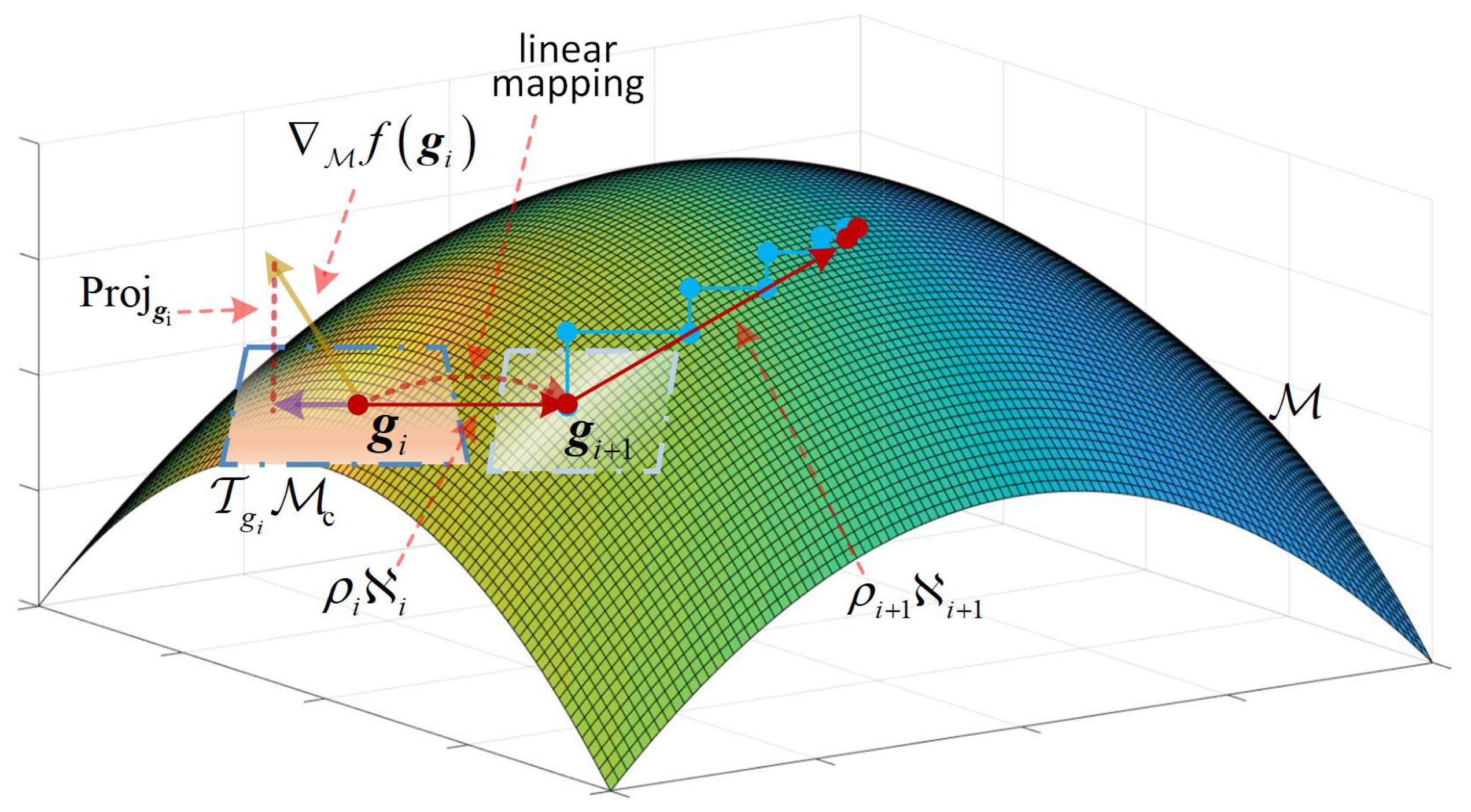
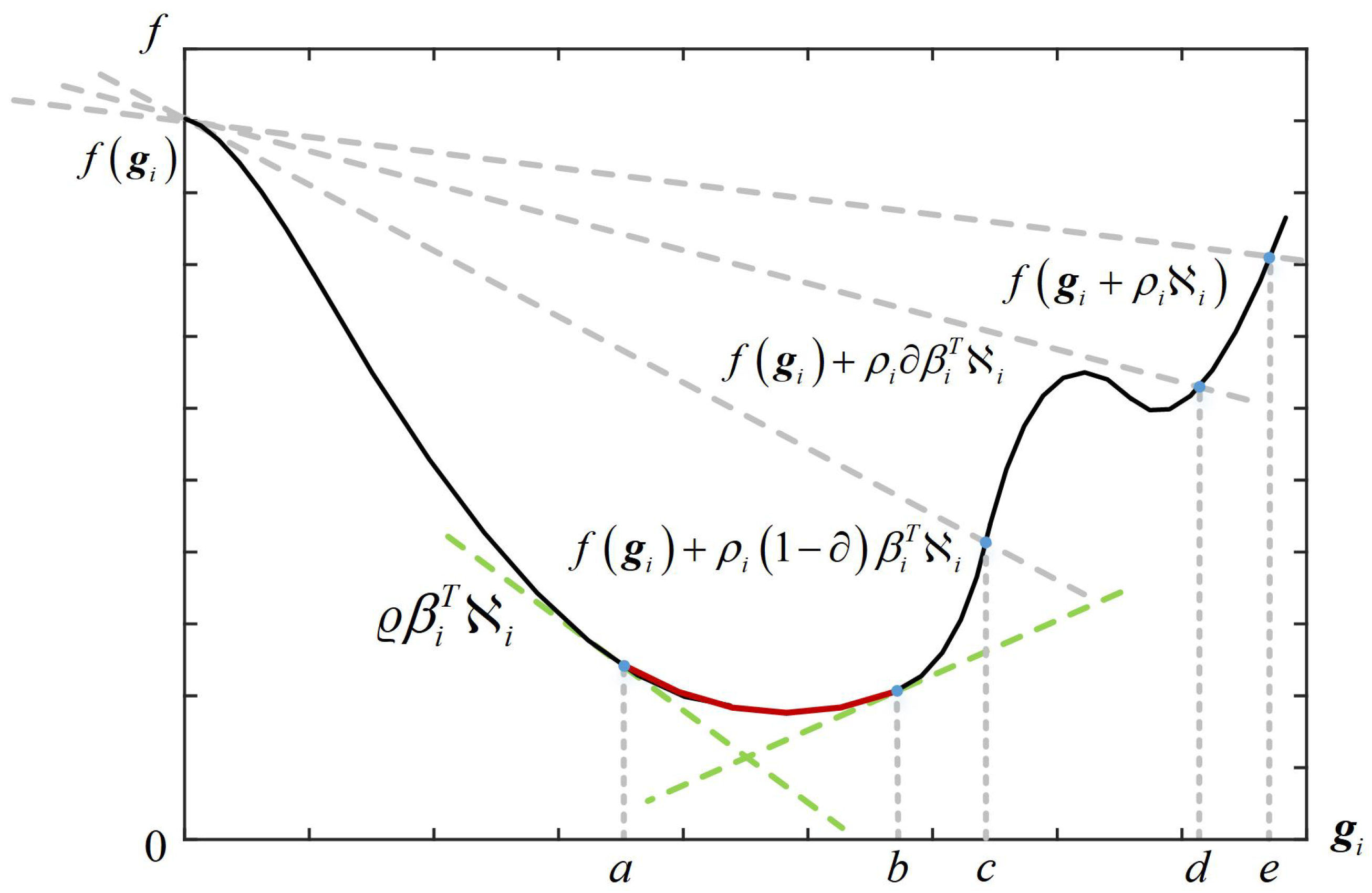
3. Solution to the Optimization Problem

As previously mentioned, the problem in (19) is nonconvex. We reformulate it as the following minimization problem:

$$\begin{array}{c}\hfill \left\{\begin{array}{c}\underset{\mathit{w},\mathbf{S}}{min}{\displaystyle \frac{{\mathit{w}}^H\left(\Psi +{\sigma }^2{\mathbf{I}}_{MK}\right)\mathit{w}}{{\left|{\sum }_{q=1}^Q{\xi }_q{\mathit{w}}^H\mathbf{S}{\mathbf{A}}_q\right|}^2}}\hfill \\ s.t.\left|{\mathbf{S}}_{n,m,k}\right|=1\hfill \end{array}\right..\end{array}$$

(20)

In order to solve the above problems, we present an AMO-NI algorithm for optimizing $\mathbf{S}$ and $\mathit{w}$ efficiently as seen in Algorithm 1. The following will describe each step of the AMO-NI algorithm.

(A)

Solution of $\mathit{w}$

To solve for $\mathit{w}$, we can transform the problem of (20) into an MVDR problem as

$$\begin{array}{c}\hfill \begin{array}{c}\underset{\mathit{w}}{min}{\displaystyle \frac{{\mathit{w}}^H\left(\Psi +{\sigma }^2{\mathbf{I}}_{MK}\right)\mathit{w}}{{\left|{\sum }_{q=1}^Q{\xi }_q{\mathit{w}}^H\mathbf{S}{\mathbf{A}}_q\right|}^2}}\hfill \end{array}.\end{array}$$

(21)

The problem in (21) has a closed-form solution. At the $t-$th iteration, the solution ${\mathit{w}}_t$ can be deduced as

$${\mathit{w}}_t={\left(\Psi +{\sigma }^2{\mathbf{I}}_{MK}\right)}^{-1}{\mathbf{S}}_{t-1}\left({\sum }_{q=1}^Q{\xi }_q{\mathbf{A}}_q\right),$$

(22)

where ${\mathbf{S}}_0$ is obtained through random initialization.

(B)

Solution of $\mathbf{S}$

In order to facilitate the discussion of question in (20), we set $\mathit{g}=vec\left(\mathbf{X}\right)\in {\mathbb{C}}^{NK\times 1}$, $\mathbf{w}=mat\left(w\right)\in {\mathbb{C}}^{M\times K}$, and $\widehat{\mathbf{w}}={\mathbf{w}}^H\otimes {\mathbf{I}}_N$, where $mat\left(\mathbf{w}\right)$ is the matricization of vector $\mathit{w}$. Under the constraint of the constant modulus, seeking $\mathit{g}$ solutions for a fixed $\widehat{\mathbf{w}}$ is challenging, so we convert the feasible domain of this problem from the Euclidean space into the Riemannian manifold. Before optimization begins, we vectorize the parameters in (20) and simplify them to

$$\begin{array}{c}\hfill \left\{\begin{array}{c}\underset{\mathit{g}}{min}{\displaystyle \frac{{\mathit{g}}^H{\widehat{\mathbf{w}}}^H{\mathbf{R}}_{\mathrm{cn}}\widehat{\mathbf{w}}\mathit{g}}{{\mathit{g}}^H{\widehat{\mathbf{w}}}^H{\mathbf{R}}_0\widehat{\mathbf{w}}\mathit{g}}}\hfill \\ s.t.\left|{\mathit{g}}_p\right|=1,p=1,\dots ,NK\hfill \end{array}\right.,\end{array}$$

(23)

where ${\mathbf{R}}_{\mathrm{cn}}={\sum }_{l=1}^L{\varpi }_l{\mathbf{B}}_l{\mathbf{B}}_l^H+{\sigma }^2{\mathbf{I}}_{NM}$ and ${\mathbf{R}}_0={\sum }_{q=1}^Q{\xi }_q{\mathit{A}}_q{\mathit{A}}_q^H$. ${\mathbf{R}}_{\mathrm{cn}}$ and ${\mathbf{R}}_0$ are covariance matrices with $NM\times NM$.

Algorithm 1 AMO-NI.

Require:  $tol={10}^{-4}$, $\epsilon ={10}^{-6}$, ${\tau }_0=10$. Ensure:  ${\mathbf{S}}^{\prime }$, ${\mathit{w}}^{\prime }$. 1: while$t\le 50$do 2:    Compute ${\mathit{w}}_t$ by (22); 3:    Initialize ${\mathbf{X}}_0\in {\mathcal{M}}_c$, 4:    ${\mathit{g}}_0=vec\left({\mathbf{X}}_0\right)$; 5:    Compute ${\eta }_0=-\nabla f\left({\mathit{g}}_0\right)$; 6:    ${\mathit{g}}_1=({\mathit{g}}_0+{\tau }_0{\eta }_0)\oslash |{\mathit{g}}_0+{\tau }_0{\eta }_0|$; 7:    $i=1$; 8:    while $i\le 1000$ do 9:        Compute ${\nabla }_{\mathcal{M}}f\left({\mathit{g}}_i\right)$ by (27) and (28); 10:      Compute ${\aleph }_i$ and ${\rho }_i$ by (29)–(31); 11:      Compute ${\mathit{g}}_{i+1}$ by (33) and (34); 12:      if $∥-{\nabla }_{\mathcal{M}}f\left({\mathit{g}}_{i+1}\right)∥\le \epsilon$ then 13:         Break; 14:      end if 15:      $i=i+1$; 16:    end while 17:    ${\mathit{w}}^{\prime }={\mathit{w}}_t$; 18:    ${\mathbf{S}}_t=mat{\left({\mathit{g}}_{i+1}\right)}^T\otimes {\mathbf{I}}_M$; 19:    ${\mathbf{S}}^{\prime }={\mathbf{S}}_t$; 20:    if $\left|{\mathrm{SIN}\mathrm{R}}_t-{\mathrm{SIN}\mathrm{R}}_{t-1}\right|\le tol$ then 21:       Break; 22:    end if 23:    $t=t+1$; 24: end while

Secondly, the nonconvex constraints related to the $\mathit{g}$ in (23) are converted into a search for the optimal solution within the complex-circles manifold. To be specific, we define a complex-circles manifold ${\mathcal{M}}_c\in {\mathbb{C}}^{NK\times 1}$ as

$$\begin{array}{c}\hfill \begin{array}{c}\hfill {\mathcal{M}}_c=\left\{\left.\mathit{g}\in {\mathbb{C}}^{NK\times 1}\right|\right.\left.\left|\mathit{g}\left(p\right)\right|=1\right\}.\end{array}\end{array}$$

(24)

Furthermore, the problem in (23) can be converted into an unconstrained optimization problem, written as

$$\underset{{\mathcal{M}}_c}{min}f\left(\mathit{g}\right)={\displaystyle \frac{{\mathit{g}}^H{\widehat{\mathbf{w}}}^H{\mathbf{R}}_{\mathrm{cn}}\widehat{\mathbf{w}}\mathit{g}}{{\mathit{g}}^H{\widehat{\mathbf{w}}}^H{\mathbf{R}}_0\widehat{\mathbf{w}}\mathit{g}}}.$$

(25)

For the problem stated in (25), we introduce an iterative loop to compute $\mathit{g}$ given $\widehat{\mathbf{w}}$. Figure 3 depicts the optimization solution process of $\mathit{g}$. In the $i-$th iteration, the tangent space is defined as

$${\mathcal{T}}_{{\mathit{g}}_i}{\mathcal{M}}_c=\left\{\mathit{b}\in {\mathbb{C}}^{NK\times 1}\left|\Re \left(\mathit{b}\odot {\mathit{g}}_i^{*}\right)=0\right.\right\},$$

(26)

The Riemannian gradient is obtained as

$$\begin{array}{c}\hfill \begin{array}{c}\hfill {\nabla }_{\mathcal{M}}f\left({\mathit{g}}_i\right)={\mathrm{Proj}}_{{\mathit{g}}_{\mathrm{i}}}\left(\nabla f\left({\mathit{g}}_i\right)\right)=\nabla f\left({\mathit{g}}_i\right)-\Re \left\{\nabla f\left({\mathit{g}}_i\right)\odot {\mathit{g}}_i^{*}\right\}\odot {\mathit{g}}_i\end{array}.\end{array}$$

(27)

Here, ${\mathrm{Proj}}_{{\mathit{g}}_i}(·)$ and $\nabla f\left({\mathit{g}}_i\right)$ are orthogonal projection operators and Euclidean gradients, respectively. When setting $\varphi ={\widehat{\mathbf{w}}}^H{\mathbf{R}}_{\mathrm{cn}}\widehat{\mathbf{w}}$ and $\upsilon ={\widehat{\mathbf{w}}}^H{\mathbf{R}}_0\widehat{\mathbf{w}}$, the Euclidean gradient $\nabla f\left({\mathit{g}}_i\right)$ can be computed by (28):

$$\begin{array}{c}\hfill \begin{array}{cc}\hfill \nabla f\left({\mathit{g}}_i\right)=& \frac{1}{{\left[{\mathit{g}}_i^H\left({\widehat{\mathbf{w}}}^H{\mathbf{R}}_0\widehat{\mathbf{w}}\right){\mathit{g}}_i\right]}^2}·\left\{\left[\left({\widehat{\mathbf{w}}}^H{\mathbf{R}}_{cn}\widehat{\mathbf{w}}\right){\mathit{g}}_i^{*}+{\left({\widehat{\mathbf{w}}}^H{\mathbf{R}}_{cn}\widehat{\mathbf{w}}\right)}^T{\mathit{g}}_i^{*}\right]\left[{\mathit{g}}_i^H\left({\widehat{\mathbf{w}}}^H{\mathbf{R}}_0\widehat{\mathbf{w}}\right){\mathit{g}}_i\right]\right.\hfill \\ \hfill & -\left.\left[\left({\widehat{\mathbf{w}}}^H{\mathbf{R}}_0\widehat{\mathbf{w}}\right){\mathit{g}}_i^{*}+{\left({\widehat{\mathbf{w}}}^H{\mathbf{R}}_0\widehat{\mathbf{w}}\right)}^T{\mathit{g}}_i^{*}\right]\left[{\mathit{g}}_i^H\left({\widehat{\mathbf{w}}}^H{\mathbf{R}}_{cn}\widehat{\mathbf{w}}\right){\mathit{g}}_i\right]\right\}\hfill \\ \hfill =& \frac{2\left({\widehat{\mathbf{w}}}^H{\mathbf{R}}_{cn}\widehat{\mathbf{w}}\right){\mathit{g}}_i^{*}}{{{\mathit{g}}_i}^H\left({\widehat{\mathbf{w}}}^H{\mathbf{R}}_0\widehat{\mathbf{w}}\right){\mathit{g}}_i}-\frac{2\left({\widehat{\mathbf{w}}}^H{\mathbf{R}}_0\widehat{\mathbf{w}}\right){\mathit{g}}_i^{*}\left[{\mathit{g}}_i^H\left({\widehat{\mathbf{w}}}^H{\mathbf{R}}_{cn}\widehat{\mathbf{w}}\right){\mathit{g}}_i\right]}{{\left({\mathit{g}}_i^H\left({\widehat{\mathbf{w}}}^H{\mathbf{R}}_0\widehat{\mathbf{w}}\right){\mathit{g}}_i\right)}^2}\hfill \\ \hfill =& \frac{2\varphi {\mathit{g}}_i^{*}}{{{\mathit{g}}_i}^H\upsilon {\mathit{g}}_i}-\frac{2\upsilon {\mathit{g}}_i^{*}\left[{\mathit{g}}_i^H\varphi {\mathit{g}}_i\right]}{{\left({\mathit{g}}_i^H\upsilon {\mathit{g}}_i\right)}^2}\hfill \end{array}\end{array}$$

(28)

On top of the Riemann gradient, we can search the steepest descent direction by the Polak–Ribiere conjugate gradient ${\aleph }_i$. ${\aleph }_i$ can be sought from

$${\aleph }_i=-{\nabla }_{\mathcal{M}}f\left({\mathit{g}}_i\right)+\Im {\mathcal{T}}_{{\mathit{g}}_{i-1}\to {\mathit{g}}_i}\mathcal{M}\left({\aleph }_{i-1}\right).$$

(29)

In (29), ℑ represents the Polak–Ribieres conjugate parameter. ${\mathcal{T}}_{{\mathit{g}}_{i-1}\to {\mathit{g}}_i}\mathcal{M}\left({\aleph }_{i-1}\right)$ denotes the linear mapping from the tangent space at ${\mathit{g}}_i$ to ${\mathit{g}}_{i+1}$. In this search, a point ${\mathit{g}}_i$ is determined, and the search direction ${\aleph }_i$ is easily obtained. Once the descent direction is obtained, the Armijo–Goldstein criterion can search for a suitable step size in most cases. However, the minimum points obtained from this method easily fall within the interval of nonminimum points. Consequently, we search for a faster-descending step using a strong Wolfe–Powell criterion [52]. The objective of the search is to find the step size ${\rho }_i$.

In the $i-$th iteration, the step size ${\rho }_i$ based on the strong Wolfe–Powell line search can be obtained by (30)–(32):

$$f\left({\mathit{g}}_i+{\aleph }_i{\rho }_i\right)\le f\left({\mathit{g}}_i\right)+{\rho }_i\partial {\beta }_i{\aleph }_i$$

(30)

$$\left|\nabla f{\left({\mathit{g}}_i+{\aleph }_i{\rho }_i\right)}^T{\aleph }_i\right|\ge -\varrho {\partial }^T{\aleph }_i$$

(31)

$${\rho }_i=-{\beta }_i{\nabla }_{\mathcal{M}}f\left({\mathit{g}}_i\right)$$

(32)

Here, ${\beta }_i\in (0,1)$, $\varrho \in (\partial ,1)$, and $\partial \in (0,1/2)$. The $f({\mathit{g}}_i)+{\rho }_i(1-\partial ){{\beta }_i}^T{\aleph }_i$ is below the second dashed line $f({\mathit{g}}_i)+{\rho }_i{{\beta }_i}^T{\aleph }_i$ due to ${\beta }_i{\aleph }_i<0$, and that is also below the first dashed line $f\left({\mathit{g}}_i+{\rho }_i{\aleph }_i\right)$ as shown in Figure 4. The first criterion in (30) is to determine whether the minimum point is within the range $\left[b,c\right]$. Due to the “stronger criterion” in (31), the slope of the tangent line is greater than or equal to $\varrho$ times the initial slope at an acceptable point. The interval of admissible points is restricted to a smaller interval $\left[d,e\right]$ containing the minimum points. The red line denotes the process wherein the objective function values are “sandwiched” or “squeezed” between the upper and lower bounds defined by the strong Wolfe–Powell criterion, ensuring an effective search for the global minimum point. We update the variable ${\mathit{g}}_i$ and assign its value to ${\mathit{g}}_{i+1}$ by

$${\tilde{\mathit{g}}}_i={\mathit{g}}_i+{\rho }_i{\aleph }_i,$$

(33)

$${\mathit{g}}_{i+1}={\tilde{\mathit{g}}}_i\oslash \left|\widetilde{{\mathit{g}}_i}\right|.$$

(34)

Finally, ${\mathbf{S}}_t$ can be updated from ${\mathbf{S}}_t={\left[mat\left({\mathit{g}}_{i+1}\right)\right]}^T\otimes {\mathbf{I}}_M$.

4. Numerical Simulations

In this section, a series of experiments are performed to verify our method’s effectiveness. Without loss of generality, we assume that all targets and interference source reflection coefficients are assumed as 1, and the noise coefficients obey a standard complex Gaussian distribution. We consider an FDA-MIMO radar with the simulation parameters as listed in

Table 1. Configuration of simulation experiment parameters.

Parameter	Value	Parameter	Value
transmitting sensors	$N=20$	range grid	181
receiving sensors	$M=20$	angle vector	[−90°,90°]
snapshot number	$K=20$	angle grid	301
frequency offset	$\Delta f=20\mathrm{kHz}$	target location	$(0^{\circ },30\mathrm{km})$
carrier frequency	$f_c=10\mathrm{Ghz}$	interference 1	$(-{50}^{\circ },10\mathrm{km})$
speed of light	$c=3\times {10}^8\mathrm{m}/\mathrm{s}$	interference 2	$({55}^{\circ },15\mathrm{km})$
inter-element spacing	$d=1/2$	interference 3	$({60}^{\circ },20\mathrm{km})$
complex coefficient	${\xi }_q={\omega }_l=1$	interference 4	$({84}^{\circ },45\mathrm{km})$
range vector	[0 km, 60 km]

. In our experiment, all numerical simulations are conducted on a computer with the Intel i7-12700F processor and 16 GB RAM, using Matlab 2018b.

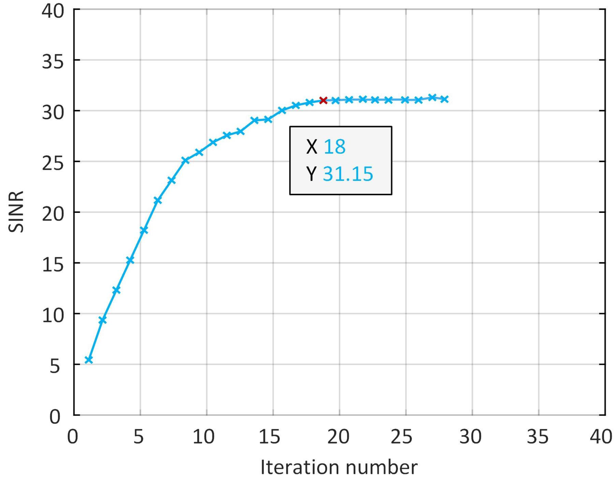
4.1. The Convergence Evaluation and Complexity Analysis

Figure 5 and Figure 6 display the Riemannian gradient norm and SINR curves as the number of iterations increases. As can be seen, (1) there is no significant fluctuation in the gradients, and (2) the value of SINR stabilizes at around 31.15 dB after about 20 iterations, reaching a converged state.

Additionally, we compare our method with some other representative optimization approaches in terms of complexity and running time as shown in

Table 2. Comparison results of complexity and runtime.

Method	Complexity (Single Iteration)	Time (s)
NCCB [53]	$\mathcal{O}(N^2+N^3{M}^3{K}^3)$	1.51
MVDR [16]	$\mathcal{O}(N^2+M^3{K}^3)$	1.29
ADMM [51]	$\mathcal{O}(M^3{K}^3+N^{3.5}{K}^{3.5})$	25.20
SDR [50]	$\mathcal{O}(M^3{K}^3+N^{3.5}{K}^{3.5}+N^2)$	0.37
ASM-ADMM [28]	$\mathcal{O}(N^2{K}^2+N^3{K}^3+N^3{K}^3+M^3{K}^3)$	543
AMO-NI (Ours)	$\mathcal{O}({\mathit{N}}^2+{\mathit{M}}^3{\mathit{K}}^3)$	0.20

. The compared optimization methods include NCCB [53], MVDR [16], ADMM [51], SDR [50], and ASM-ADMM [28]. It can be observed that (1) in a single iteration, the complexity of the proposed method is $\mathcal{O}(M^3{K}^3+N^2)$, which is lower than other methods. (2) The algorithm’s running time is 0.2 s, faster than others.

All this demonstrates the excellent performance of our algorithm in terms of stability and efficiency. We attribute these promising results to the fact that (i) our method reduces the complexity of the optimization for $\mathbf{S}$ as shown in (24), (ii) our method is a 2D search in manifold and possesses a faster convergence rate (see Figure 5), and (iii) our method avoids convex relaxation and extensive matrix eigenvalue decomposition, thus speeding up the solution process.

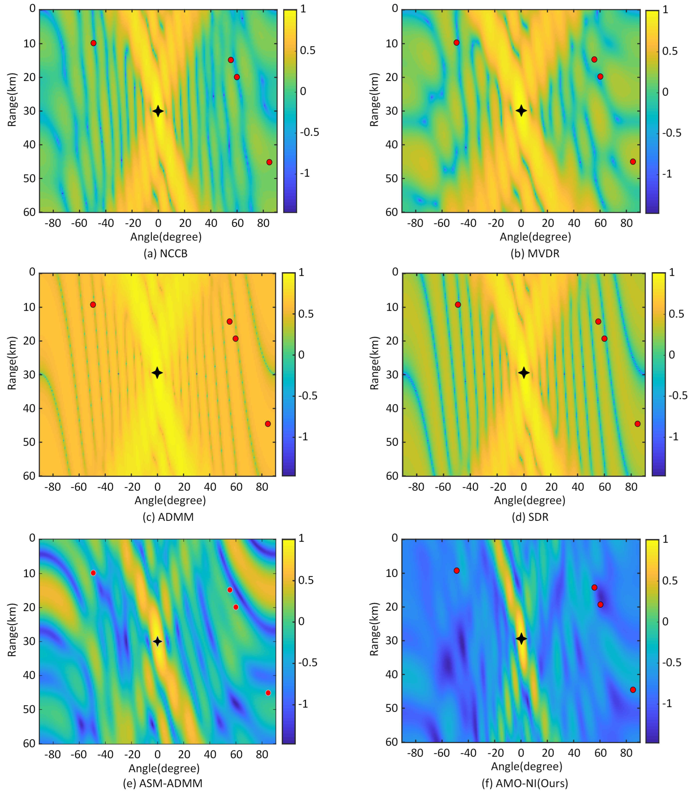
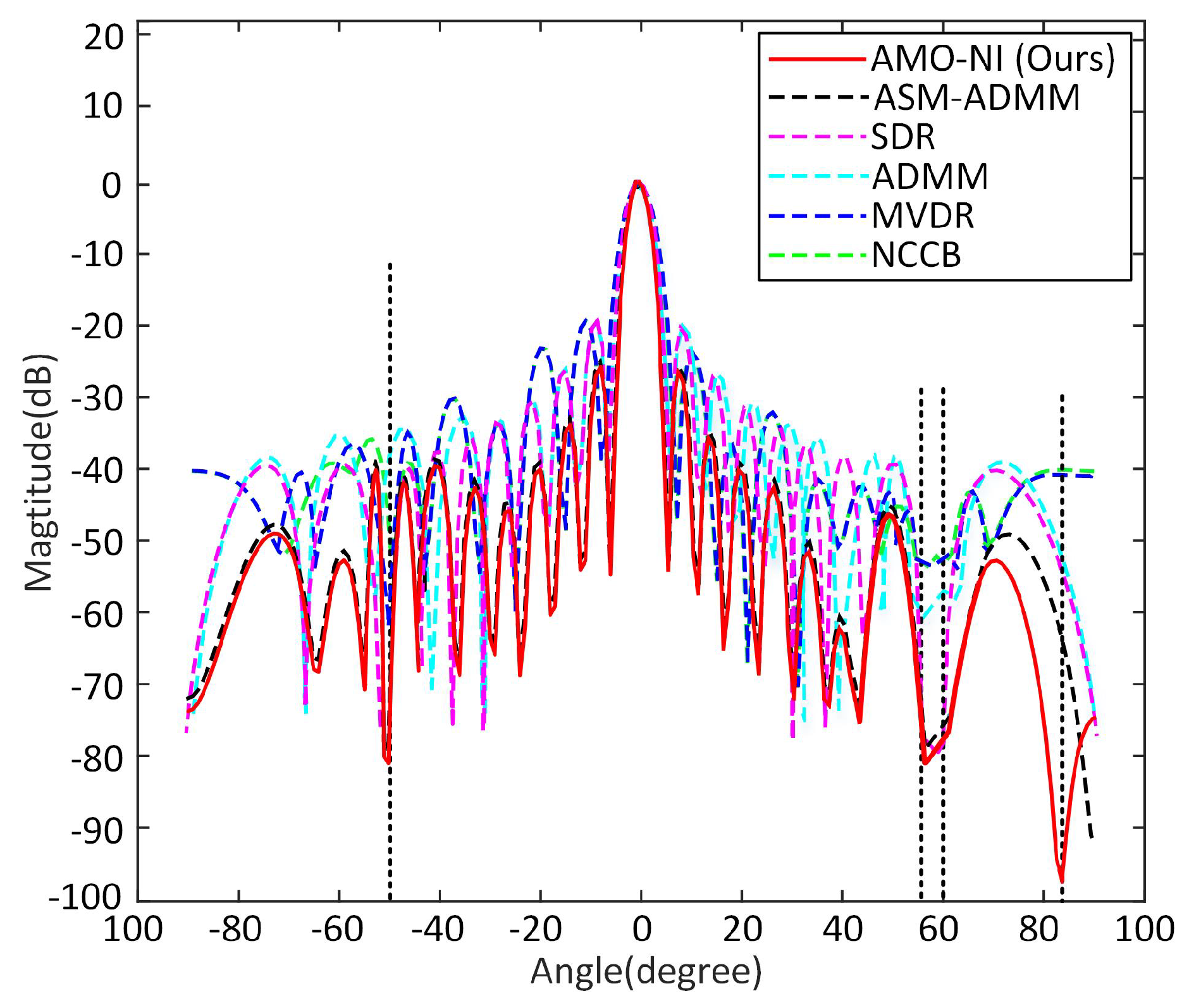
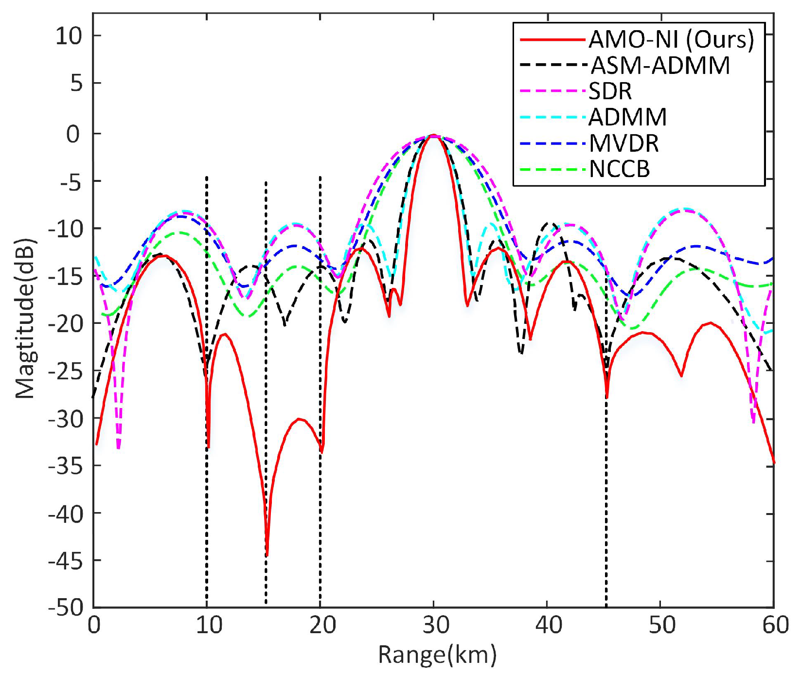
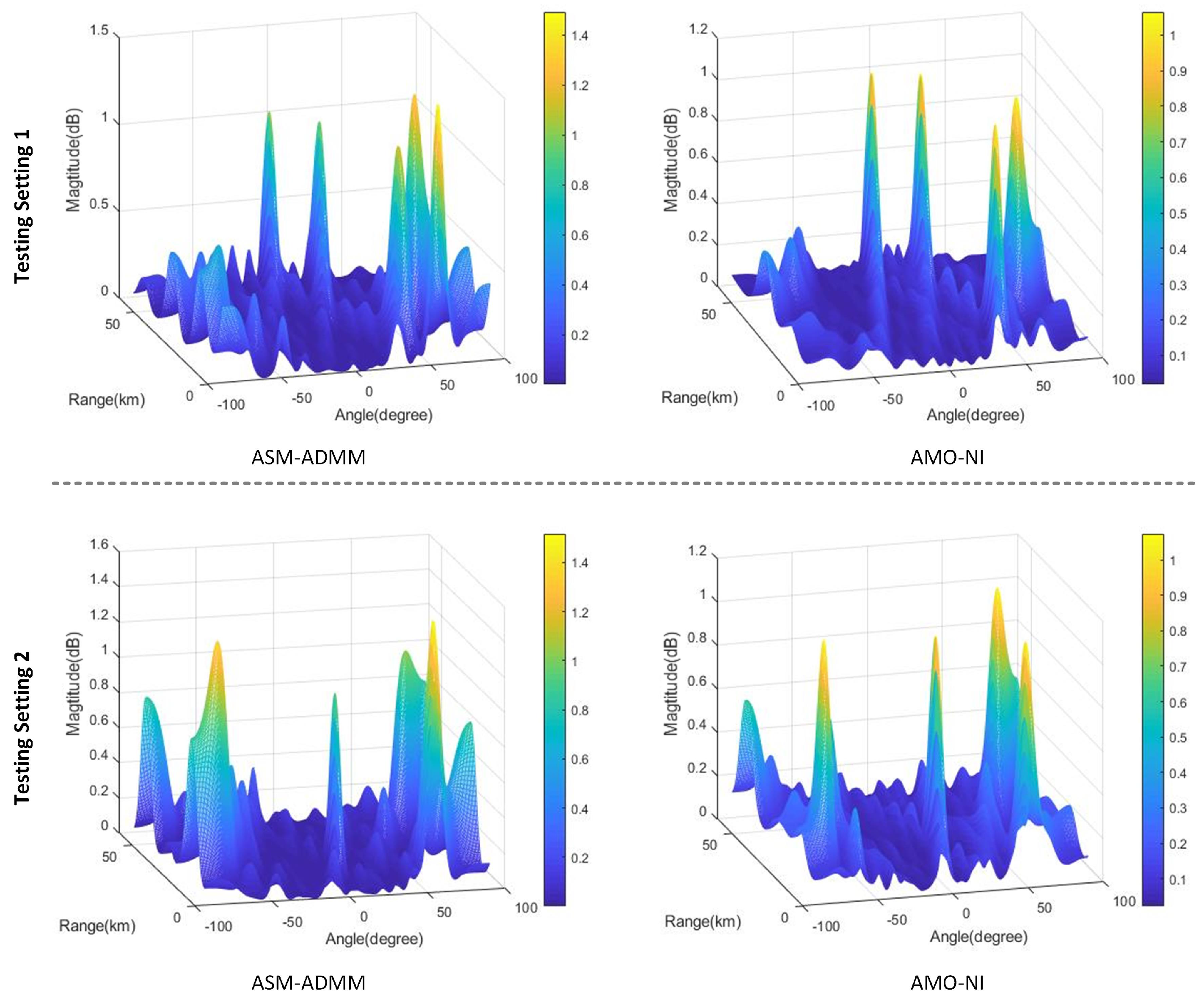
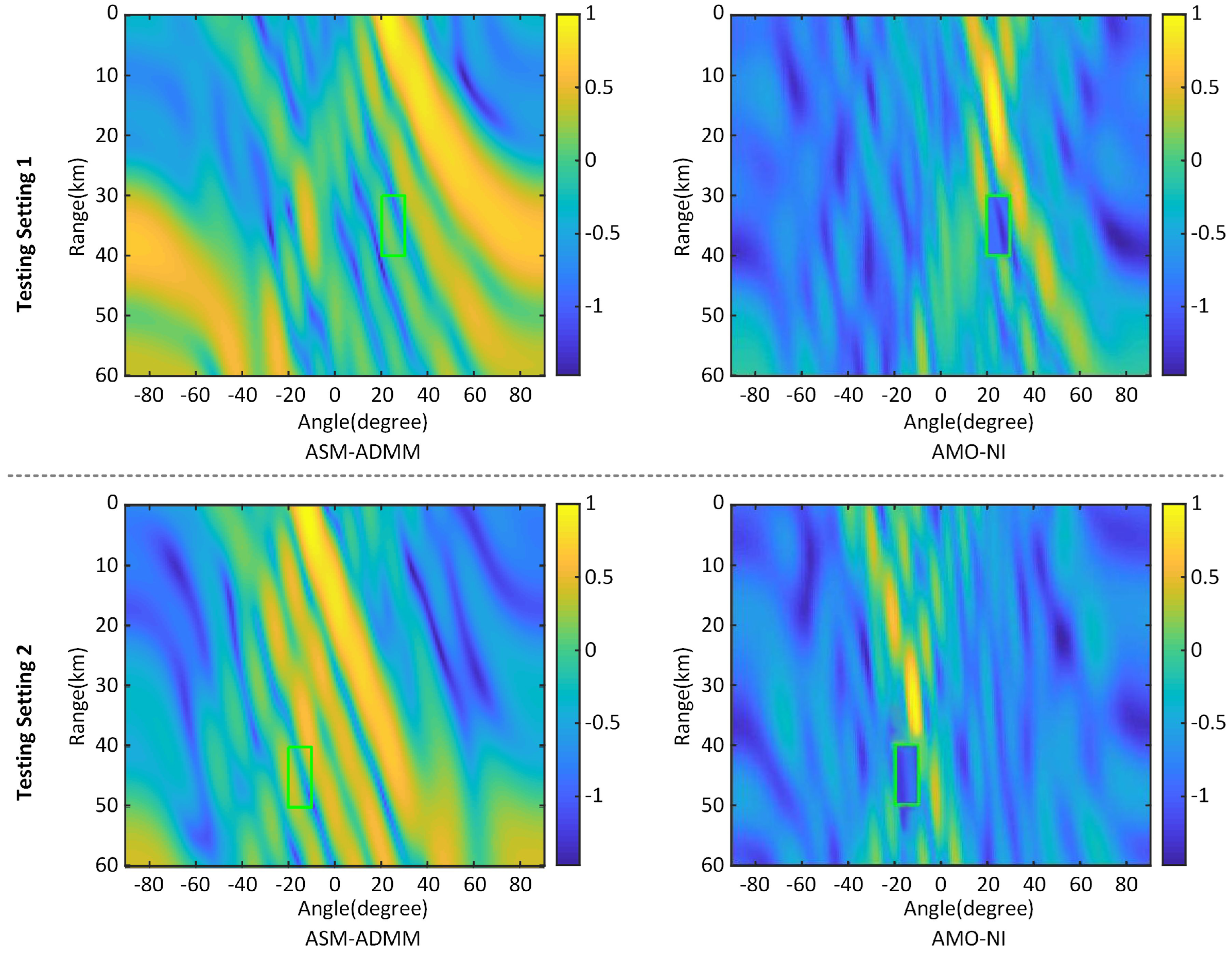
4.2. Results of Transceiver Beampattern

We compare our method with other schemes in half-power widths, 2D-beampatterns, as well as range and angle profiles. The comparison results are presented in

Table 3. Comparison results of half-power width. ↓ indicates better performance with lower values.

Method	Half-Power Width
	Angle (Degree) ↓	Range (km) ↓
NCCB [53]	6.0	14.2
MVDR [16]	10.0	35.0
ADMM [51]	4.0	9.4
SDR [50]	87.0	16.9
ASM-ADMM [28]	5.7	10.8
AMO-NI (Ours)	3.6	8.9

. Our algorithm achieves the narrowest half-power widths (3.6 degrees and 8.9 km). This indicates that the proposed method possesses superior capabilities in beam focusing and decoupling.

Figure 7 presents the 2D beampatterns of our method and other ones. With the same configuration, our method generates beampatterns that effectively point towards the target center (refer to the highlighted regions at the black four-pointed stars) than other methods, including NCCB, MVDR, ADMM, SDR, and ASM-ADMM. Meanwhile, our method better suppresses the generation of X-shaped beampatterns and has deeper nulling at the interferences (blue regions at red points). All these indicate that our method could form a beampattern with a lower sidelobe level, less scattering, and more concentrated energy. We attribute these superiorities primarily to our use of a maximized SINR objective function in optimizing the transmit and receive beamforming variables, which maximizes the power indication to the target while minimizing the beam power in the direction of interference.

In Figure 8, we show the results of different optimization methods in terms of angle profiles. Our approach achieves deeper and more accurate nulling in the angle profile among all algorithms under the same setting. To be specific, our AMO-NI obtains the lowest nulling (about −95 dB), which significantly beats the strongest competitor ASM-ADMM. This implies that the proposed method effectively directs the beam towards desired directions while suppressing undesired ones, which is consistent with the conclusions drawn from the observations in Figure 7 and demonstrates that optimizing the transmit waveform and receive filter weights could enhance the accuracy of beamforming in angle once again.

As shown in Figure 9, the performance in the range profile is also consistent. Our method has narrower mainlobe width and faster sidelobe attenuation than others. At the range profile, a minimum nulling of −45 dB is achieved at the interference region, notably surpassing the best-performing method SDR (−45 dB vs. −33 dB). This indicates that our method exhibits better directionality in the range dimension and possesses greater potential for interference suppression. We argue that these advances in range dimension mainly benefit from iteratively optimizing and coordinating subproblems to obtain the global optimal solution.

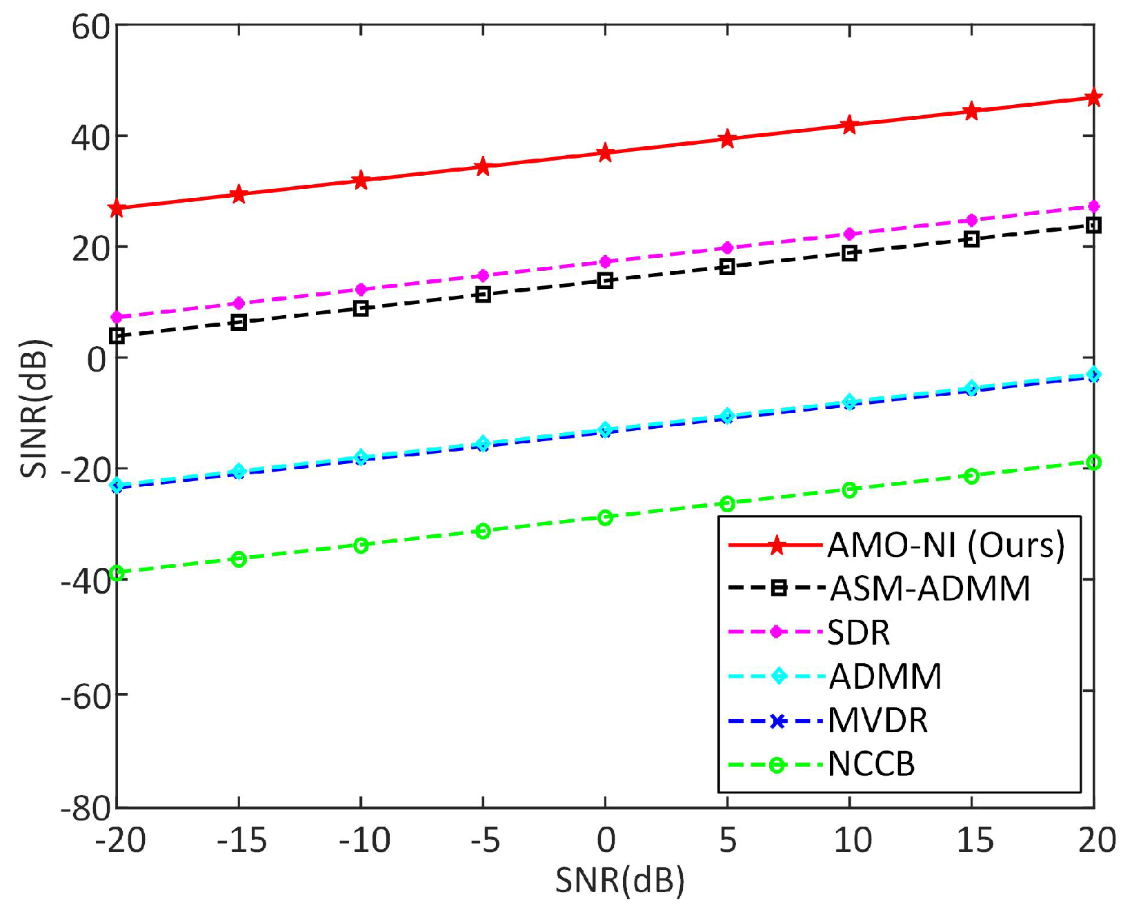
4.3. Results of SINR

In Figure 10, we present the output SINR versus transmit SNR for our method and other approaches. Our method achieves the highest output SINR, surpassing NCCB [53], MVDR [16], ADMM [51], SDR [50], and ASM-ADMM [28] by 64 dB, 48 dB, 48 dB, 18 dB, and 21.3 dB, respectively. Those results demonstrate that our AMO-NI has higher signal quality and availability of communication in FDA-MIMO radar systems.

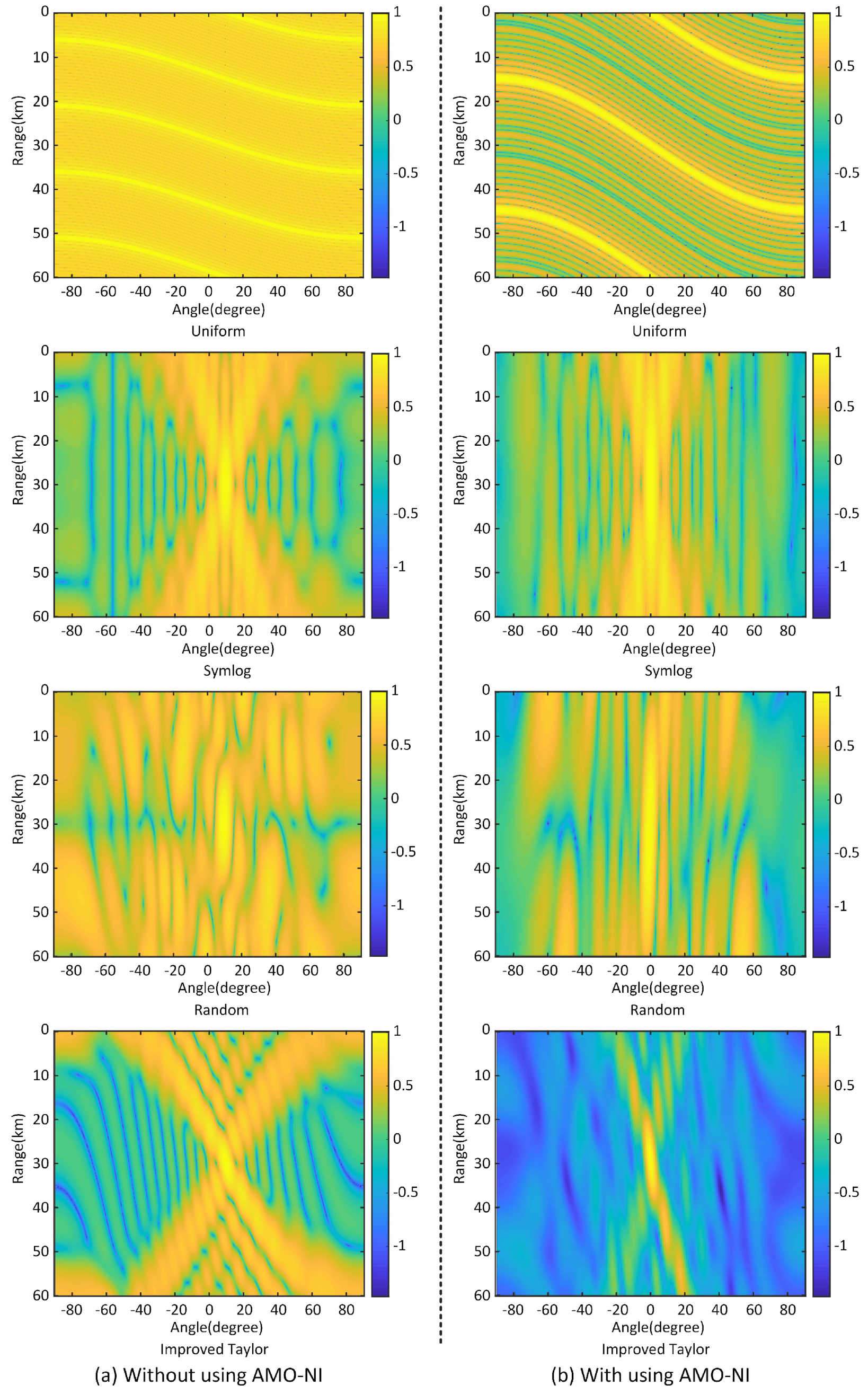
4.4. Effects of Frequency Offset Configuration on Beamforming

We analyze the changes before and after using our beamforming method at different frequency offsets.

Table 4. Half-power width test at different frequency offsets with and without AMO-NI.

Frequency Offsets	Half-Power Width without AMO-NI		Half-Power Width with AMO-NI
	Angle (Degree)	Range (km)	Angle (Degree)	Range (km)
Uniform [39]	22	1.2	3.6	0.3
Symlog [34]	22	24.8	3.6	22
Random [54]	22	26.8	3.6	22
Improved Taylor [35]	22	11.2	3.6	8.9

presents half-power widths of the beampattern in range and angle dimensions with and without AMO-NI at various frequency offset configurations, including uniform, symmetric logarithmic, random, and improved Taylor window function. As observed, after applying AMO-NI, the half-power width in the angle dimension decreases from 22 degrees to 3.6 degrees under different frequency offsets, and a competitive half-power width of 8.9 km is achieved in the range dimension with the improved Taylor frequency offset. Here, the uniform frequency offset is not discussed due to its serious range–angle coupling. The above results demonstrate that frequency offsets have a minimal impact on the half-power width in the angle dimension but significantly affect it in the range dimension. This is consistent with the fact that the primary parameters affecting the range dimension resolution in the FDA-MIMO radar are frequency offset and bandwidth, and the nonlinear frequency offset configuration can decouple the range and angle. On the other hand, we find a significant reduction in the half-power widths with our AMO-NI. This reduction is primarily attributed to the optimization of transmit sequences and receiver filter weights, resulting in a decrease in the bandwidth.

Figure 11 depicts transceiver beampatterns with and without AMO-NI under various frequency offsets. The first row in Figure 11 exhibits S-shaped beampatterns with periodic appearance at the target (see yellow highlights), which indicates range–angle coupling. Without employing AMO-NI, X-shaped beampatterns with dot-shaped yellow highlights at the target and increased scattering are presented as seen in the leftmost rows 2 to 4 of Figure 11. These X-shaped beampatterns are decoupling, but their beam focusing is inadequate and spectral leakage is serious. Conversely, the scattering of the beampatterns after applying AMO-NO (see right rows of 2 to 4 in Figure 11) is notably diminished, and optimal focusing performance is demonstrated (see right last row). This improvement is attributed to the optimization algorithm modifying the transmitted beam space matrix, thus partially reducing beam illumination power towards nontarget areas.

4.5. Extended Experiments

Beyond high-quality beamforming in the FDA-MIMO radar, we extend our method AMO-NI to additional test cases, such as multi-beam generation in a drone swarm and swarm interference suppressing in mainlobe. For comparison in these two cases, we select a competitive algorithm named ASM-ADMM as the baseline. Next, the experiment configuration and results of each test case are presented, respectively.

Multi-beam generation in drone swarm: Tracking the drone swarm with slow or uniform motion poses a challenge [55]. To evaluate the generality of our method in such a challenging scenario, an ideal environment with open space and clear weather is considered, where the angles and ranges of the drone swarm are randomly generated within ${\Theta }_Q=\left\{\left.\left({\theta }_q,r_q\right)\right|-{90}^{\circ }\le {\theta }_q\le {90}^{\circ },0\mathrm{km}\le r_q\le 60\mathrm{km}\right\}$.

We utilize the proposed algorithm AMO-NI to synthesize multiple beams to indicate the direction of each drone. There are two testing settings (i.e., ${\mathbb{X}}_1$ and ${\mathbb{X}}_2$) randomly generated, each comprising four targets with their angles and ranges as follows:

$$\left\{\begin{array}{c}{\mathbb{X}}_1=\left\{\left({23.5}^{\circ },47.2\mathrm{km}\right),\left(-{3.7}^{\circ },54.8\mathrm{km}\right),\left({68.3}^{\circ },28.9\mathrm{km}\right),\left({41.7}^{\circ },14.2\mathrm{km}\right)\right\}\hfill \\ {\mathbb{X}}_2=\left\{\left({56.6}^{\circ },9.7\mathrm{km}\right),\left({73.4}^{\circ },47.7\mathrm{km}\right),\left(-{67.1}^{\circ },18.3\mathrm{km}\right),\left({8.4}^{\circ },22\mathrm{km}\right)\right\}\hfill \end{array}\right..$$

(35)

As shown in Figure 12, we present the comparison results of our method AMO-NI and ASM-ADMM in the 3D normalized power spectrum. Our AMO-NI produces clear main beams at the four targets, whereas ASM-ADMM shows noticeable false peaks and fails to distinguish these main peaks. Additionally, in the same test settings, compared with ASM-ADMM, our proposed algorithm demonstrates good performance in both the range and angle resolution, especially within the degree intervals $[-{90}^{\circ },-{70}^{\circ }]$ and $[{70}^{\circ },{90}^{\circ }]$, with lower sidelobes in nontarget regions. The results demonstrate that (i) our algorithm can effectively synthesize multiple beams, and (ii) the beams synthesized by our algorithm have higher spectral efficiency. These phenomena are consistent with the analysis in Section 2.2 and the results in Section 4.2, suggesting the generality of our approach to multi-beam generation in drone swarm.

Swarm interference suppressing in mainlobe: Swarm interference is very common in real-world applications [6,12]. Assuming that prior knowledge of both the interference sources and the targets can be obtained, we synthesize the main beams to indicate target positions, forming nulls in the interference regions. The target and swarm interference powers are set to 10 dB and 30 dB, respectively. To verify the robustness of the proposed algorithm suppressing swarm interference at the same angle, we conducted two testing settings. In the first testing setting, the target is randomly located at $\left({\theta }_{q1},r_{q,1}\right)=\left\{23.2^{\circ },15.6\mathrm{km}\right\}$, and the six swarm interference is randomly distributed in area ${\Theta }_{J,1}=\left\{\left.\left({\theta }_{j,1},r_{j,1}\right)\right|{20}^{\circ }\le {\theta }_{j,1}\le {30}^{\circ },30\mathrm{km}\le r_{j,1}\le 40\mathrm{km}\right\}$. The details of the interference sources are as follows:

$${\Theta }_{J,1}=\left\{\begin{array}{c}\left(20.7^{\circ },38.1\mathrm{km}\right),(29.5^{\circ },34.9\mathrm{km}),\left(22.9^{\circ },39.4\mathrm{km}\right),\hfill \\ (26.4^{\circ },30.2\mathrm{km}),\left(24.0^{\circ },31.8\mathrm{km}\right),(21.6^{\circ },37.5\mathrm{km})\hfill \end{array}\right\}.$$

(36)

In the second testing setting, we randomly generate the target coordinate $\left({\theta }_{q,2},r_{q,2}\right)$$=\left\{-11.7^{\circ },33.5\mathrm{km}\right\}$, and the swarm interference coordinates within ${\Theta }_{J,2}=\left\{\left.\left({\theta }_{j,2},r_{j,2}\right)\right|\right.$$\left.-{20}^{\circ }\le {\theta }_{j,2}\le -{10}^{\circ },40\mathrm{km}\le r_{j,2}\le 50\mathrm{km}\right\}$. The interference coordinates randomly generated are

$${\Theta }_{J,1}=\left\{\begin{array}{c}\left(-13.7^{\circ },43.5\mathrm{km}\right),(-12.9^{\circ },46.3\mathrm{km}),\left(-15.2^{\circ },44.8\mathrm{km}\right),\hfill \\ (-17.8^{\circ },41.9\mathrm{km}),\left(-11.4^{\circ },48.2\mathrm{km}\right),(-11.9^{\circ },49.7\mathrm{km})\hfill \end{array}\right\}.$$

(37)

As shown in Figure 13, our AMO-NI shows clear focusing at target positions (yellow regions) and deep nulling in the interference areas (green rectangles). In contrast, ASM-ADMM shows poor focusing at target positions and lacks nulling in the interference areas. This indicates the superiority and potential of our method for swarm interference suppressing in the mainlobe. We attribute the superiority of our algorithm to the fact that our optimization method effectively improves the range resolution and suppresses the spectral energy in the interference region.

5. Conclusions

This paper proposes an efficient optimization algorithm, termed AMO-NI, to address the problem of joint transceiver beamforming in the FDA-MIMO radar. Firstly, we derive the generalized ambiguity function of the FDA-MIMO radar and conclude that optimized transceiver beamforming can reduce the bandwidth, improving range resolution. Upon this investigation, we formulate the transceiver beampattern optimization as a nonconvex bivariate quadratic programming problem (NBQP). To tackle the NBQP while ensuring the solution’s optimality for transmit waveform and receive filter weight, an innovative alternating manifold optimization algorithm is proposed. In the experiments, our algorithm demonstrates higher operational efficiency (0.2 s), capable of generating more focused beampattern, with a half-power width of 3.6 degrees in angle and 8.9 km in range, as well as surpassing the closest competitor, ASM-ADMM, by 21.3 dB in the system SINR.

Our method has achieved promising results in beamforming. However, an interesting fact worth exploring is the collaboration of our algorithm with parameter estimation to achieve robust target detection.

References

1. Ding, Z.; Xie, J.; Xu, J. A Joint Array Parameters Design Method Based on FDA-MIMO Radar. IEEE Trans. Aerosp. Electron. Syst. 2023, 59, 2909–2919. [Google Scholar] [CrossRef]
2. Liu, Q.; Wang, X.; Huang, M.; Lan, X.; Sun, L. DOA and Range Estimation for FDA-MIMO Radar with Sparse Bayesian Learning. Remote Sens. 2021, 13, 2553. [Google Scholar] [CrossRef]
3. Huang, B.; Wang, W.; Basit, A.; Gui, R. Bayesian Detection in Gaussian Clutter for FDA-MIMO Radar. IEEE Trans. Veh. Technol. 2022, 71, 2655–2667. [Google Scholar] [CrossRef]
4. Tian, X.; Chen, H.; Huang, B.; Wang, W.Q. Fast Parameter Estimation Algorithms for Conformal FDA-MIMO Radar. IEEE Sens. J. 2023, 23, 30633–30641. [Google Scholar] [CrossRef]
5. Lan, L.; Xu, J.; Liao, G.; Zhang, Y.; Fioranelli, F.; So, H.C. Suppression of Mainbeam Deceptive Jammer With FDA-MIMO Radar. IEEE Trans. Veh. Technol. 2020, 69, 11584–11598. [Google Scholar] [CrossRef]
6. Wu, Z.; Zhu, S.; Xu, J.; Lan, L.; Zhang, M. Interference Suppression Method With MR-FDA-MIMO Radar. IEEE Trans. Aerosp. Electron. Syst. 2023, 59, 6250–6264. [Google Scholar] [CrossRef]
7. Wang, K.; Liao, G.; Xu, J.; Zhang, Y.; Lan, L.; Wang, W. Multi-scale moving target detection with FDA-MIMO radar. Signal Process. 2024, 216, 109301. [Google Scholar] [CrossRef]
8. Lan, L.; Liao, G.; Xu, J.; Zhu, S.; Zhang, Y. Range-angle-dependent beamforming for FDA-MIMO radar using oblique projection. Sci. China Inf. Sci. 2022, 65, 152305. [Google Scholar] [CrossRef]
9. Yu, L.; He, F.; Zhang, Y.; Su, Y. Low-PSL Mismatched Filter Design for Coherent FDA Radar Using Phase-Coded Waveform. IEEE Geosci. Remote Sens. Lett. 2023, 20, 3507405. [Google Scholar] [CrossRef]
10. Akkoc, A.; Korkmaz, N.A.; Genc, Y.; Afacan, E.; Yazgan, E. Time-Invariant and Localized Secure Reception With Sequential Multicarrier Receive-FDA. IEEE Trans. Antennas Propag. 2023, 71, 7064–7072. [Google Scholar] [CrossRef]
11. Jia, W.; Jakobsson, A.; Wang, W.Q. Optimal Frequency Offset Selection for FDA-MIMO Beampattern Design in the Range-Angle Plane. IEEE Signal Process. Lett 2023, 31, 316–320. [Google Scholar] [CrossRef]
12. Chen, G.; Wang, C.; Gong, J.; Tan, M.; Liu, Y. Data-Independent Phase-Only Beamforming of FDA-MIMO Radar for Swarm Interference Suppression. Remote Sens. 2023, 15, 1159. [Google Scholar] [CrossRef]
13. Li, J.; Liao, G.; Huang, Y.; Zhang, Z.; Nehorai, A. Riemannian Geometric Optimization Methods for Joint Design of Transmit Sequence and Receive Filter on MIMO Radar. IEEE Trans. Signal Process. 2020, 68, 5602–5616. [Google Scholar] [CrossRef]
14. Zhang, Z.; Wen, F.; Shi, J.; He, J.; Truong, T.K. 2D-DOA Estimation for Coherent Signals via a Polarized Uniform Rectangular Array. IEEE Signal Process. Lett. 2023, 30, 893–897. [Google Scholar] [CrossRef]
15. Zhang, Z.; Shi, J.; Wen, F. Phase Compensation-based 2D-DOA Estimation for EMVS-MIMO Radar. IEEE Trans. Aerosp. Electron. Syst. 2023; 1–10. [Google Scholar]
16. Chalise, B.K.; Amin, M.G.; Martone, A.; Kirk, B.; Sherbondy, K. Optimum Hybrid MVDR Beamformer With Sparse Signal Recovery Approach. In Proceedings of the 2022 IEEE Radar Conference (RadarConf22), New York, NY, USA, 21–25 March 2022; pp. 1–6. [Google Scholar]
17. He, Q.; He, Z.; Wang, Z.; Peng, W. Co-Design of Transmit-Receive Weights for MIMO System With LPI and Multi-Targets. IEEE Commun. Lett. 2022, 26, 1863–1867. [Google Scholar] [CrossRef]
18. Zhai, Y.; Li, X.; Hu, J.; Zhong, K. The Transmit Beampattern Design in MIMO Radar System: A Manifold Optimization based Method. In Proceedings of the 2022 IEEE Radar Conference (RadarConf22), New York, NY, USA, 21–25 March 2022; pp. 1–5. [Google Scholar]
19. Xiong, J.; Wang, W.Q.; Gao, K. FDA-MIMO Radar Range–Angle Estimation: CRLB, MSE, and Resolution Analysis. IEEE Trans. Aerosp. Electron. Syst. 2018, 54, 284–294. [Google Scholar] [CrossRef]
20. Johnston, J.; Venturino, L.; Grossi, E.; Lops, M.; Wang, X. Waveform and Filter Design in MIMO OFDM Dual-Function Radar-Communication. In Proceedings of the 2022 IEEE Radar Conference (RadarConf22), New York, NY, USA, 21–25 March 2022; pp. 1–6. [Google Scholar]
21. Zhang, R.; Chen, Y.; Gu, M.; Sheng, W. Synthesis of Directional Modulation LFM Radar Waveform for Sidelobe Jamming Suppression. IEEE Sens. J. 2023, 23, 28055–28066. [Google Scholar] [CrossRef]
22. Ding, Z.; Xie, J. Joint Transmit and Receive Beamforming for Cognitive FDA-MIMO Radar With Moving Target. IEEE Sens. J. 2021, 21, 20878–20885. [Google Scholar] [CrossRef]
23. Dong, F.; Wang, W.; Li, X.; Liu, F.; Chen, S.; Hanzo, L. Joint Beamforming Design for Dual-Functional MIMO Radar and Communication Systems Guaranteeing Physical Layer Security. IEEE Trans. Green Commun. Netw. 2023, 7, 537–549. [Google Scholar] [CrossRef]
24. Nishihara, R.; Lessard, L.; Recht, B.; Packard, A.; Jordan, M. A general analysis of the convergence of ADMM. In Proceedings of the ICML’15: Proceedings of the 32nd International Conference on International Conference on Machine Learning, PMLR, Lille, France, 6–11 July 2015; pp. 343–352.
25. Yu, X.; Qiu, H.; Yang, J.; Wei, W.; Cui, G.; Kong, L. Multispectrally Constrained MIMO Radar Beampattern Design via Sequential Convex Approximation. IEEE Trans. Aerosp. Electron. Syst. 2022, 58, 2935–2949. [Google Scholar] [CrossRef]
26. Xu, Y.; Li, Y.; Zhang, J.A.; Di Renzo, M.; Quek, T.Q.S. Joint Beamforming for RIS-Assisted Integrated Sensing and Communication Systems. IEEE Trans. Commun. 2023; 1–14. [Google Scholar]
27. Basit, A.; Wang, W.Q.; Wali, S.; Yaw Nusenu, S. Transmit beamspace design for FDA–MIMO radar with alternating direction method of multipliers. Signal Process. 2021, 180, 107832. [Google Scholar] [CrossRef]
28. Gong, P.; Zhang, Z.; Wu, Y.; Wang, W.Q. Joint Design of Transmit Waveform and Receive Beamforming for LPI FDA-MIMO Radar. IEEE Signal Process. Lett. 2022, 29, 1938–1942. [Google Scholar] [CrossRef]
29. Lan, L.; Liao, G.; Xu, J.; Zhang, Y.; Liao, B. Transceive Beamforming With Accurate Nulling in FDA-MIMO Radar for Imaging. IEEE Trans. Geosci. Remote Sens. 2020, 58, 4145–4159. [Google Scholar] [CrossRef]
30. Wang, W.Q.; Dai, M.; Zheng, Z. FDA Radar Ambiguity Function Characteristics Analysis and Optimization. IEEE Trans. Aerosp. Electron. Syst. 2018, 54, 1368–1380. [Google Scholar] [CrossRef]
31. Ma, Y.; Wei, P.; Zhang, H. General Focusing Beamformer for FDA: Mathematical Model and Resolution Analysis. IEEE Trans. Antennas Propag. 2019, 67, 3089–3100. [Google Scholar] [CrossRef]
32. Gui, R.; Huang, B.; Wang, W.Q.; Sun, Y. Generalized Ambiguity Function for FDA Radar Joint Range, Angle and Doppler Resolution Evaluation. IEEE Geosci. Remote Sens. Lett. 2022, 19, 3502305. [Google Scholar] [CrossRef]
33. Bang, H.; Wang, W.Q.; Zhang, S.; Liao, Y. FDA-Based Space–Time–Frequency Deceptive Jamming Against SAR Imaging. IEEE Trans. Aerosp. Electron. Syst. 2022, 58, 2127–2140. [Google Scholar] [CrossRef]
34. Liao, Y.; Tang, H.; Chen, X.; Wang, W.Q. Frequency Diverse Array Beampattern Synthesis with Taylor Windowed Frequency Offsets. IEEE Antennas Wirel. Propag. Lett. 2020, 19, 1901–1905. [Google Scholar] [CrossRef]
35. Langhuan, G.; Youg, L.; Wei, C.; Limeng, D.; Yumei, T. Highly focussed beampattern synthesis in FDA-MIMO radar with multicarrier transmission. IET Radar Sonar Navig. 2023, 17, 665–682. [Google Scholar]
36. Tan, M.; Gong, J.; Wang, C. Range Dimensional Monopulse Approach With FDA-MIMO Radar for Mainlobe Deceptive Jamming Suppression. IEEE Antenn. Wirel. Propag. Lett. 2024, 23, 643–647. [Google Scholar] [CrossRef]
37. Xu, J.; Liao, G.; Zhang, Y.; Ji, H.; Huang, L. An Adaptive Range-Angle-Doppler Processing Approach for FDA-MIMO Radar Using Three-Dimensional Localization. IEEE J. Sel. Top. Signal Process. 2017, 11, 309–320. [Google Scholar] [CrossRef]
38. Huang, B.; Jian, J.; Basit, A.; Gui, R.; Wang, W.Q. Adaptive Distributed Target Detection for FDA-MIMO Radar in Gaussian Clutter Without Training Data. IEEE Trans. Aerosp. Electron. Syst. 2022, 58, 2961–2972. [Google Scholar] [CrossRef]
39. Tan, M.; Wang, C.; Li, Z. Correction Analysis of Frequency Diverse Array Radar about Time. IEEE Trans. Antennas Propag. 2021, 69, 834–847. [Google Scholar] [CrossRef]
40. Zhou, C.; Wang, C.; Gong, J.; Tan, M.; Bao, L.; Liu, M. Ambiguity Function Evaluation and Optimization of the Transmitting Beamspace-Based FDA Radar. Signal Process. 2023, 203, 108810. [Google Scholar] [CrossRef]
41. Wen, H.; Gu, P.; He, Z.; Lian, J.; Wang, J.; Song, D.; Ding, D.z. Optimal Function-based Frequency Offset Design Based on Polynomial Fitting for Frequency Diverse Array Beampattern Synthesis. IEEE Antenn. Wirel. Propag. Lett. 2023, 23, 149–153. [Google Scholar] [CrossRef]
42. Jian, J.; Wang, W.; Huang, B.; Zhang, L.; Imran, M.A.; Huang, Q. MIMO-FDA Communications with Frequency Offsets Index Modulation. IEEE Trans. Wireless Commun. 2023; 1–15. [Google Scholar]
43. Zhu, Z.; Chen, W.; Yang, Y.; Shu, Q. Frequency Diverse Array Beampattern Synthesis with Random Permutated Power Increasing Frequency Offset. IEEE Antennas Wirel. Propagat. Lett. 2022, 21, 1975–1979. [Google Scholar] [CrossRef]
44. Cheng, X.; Wu, L.; Ciuonzo, D.; Wang, W. Joint Design of Horizontal and Vertical Polarization Waveforms for Polarimetric Radar via SINR Maximization. IEEE Trans. Aerosp. Electron. Syst. 2023, 59, 3313–3328. [Google Scholar] [CrossRef]
45. Yao, Y.; Li, Z.; Liu, H.; Miao, P.; Wu, L. Robust Transceiver Optimization Against Echo Eclipsing via Majorization-Minimization. IEEE Trans. Aerosp. Electron. Syst. 2023, 59, 2464–2479. [Google Scholar] [CrossRef]
46. Aghashahi, S.; Zeinalpour-Yazdi, Z.; Tadaion, A.; Mashhadi, M.B.; Elzanaty, A. MU-Massive MIMO with Multiple RISs: SINR Maximization and Asymptotic Analysis. IEEE Wirel. Commun. Lett. 2023, 12, 997–1001. [Google Scholar] [CrossRef]
47. Chu, C.; Chen, Y.; Luo, Y.; Zhang, Q. Wideband MIMO Radar Waveform Design under Multiple Criteria. IEEE Geosci. Remote Sens. Lett. 2023, 20, 3506305. [Google Scholar] [CrossRef]
48. Raei, E.; Sedighi, S.; Alaee-Kerahroodi, M.; Bhavani Shankar, M.R. MIMO Radar Transmit Beampattern Shaping for Spectrally Dense Environments. IEEE Trans. Aerosp. Electron. Syst. 2023, 59, 1007–1020. [Google Scholar] [CrossRef]
49. Alhujaili, K.; Yu, X.; Cui, G.; Monga, V. Spectrally Compatible MIMO Radar Beampattern Design under Constant Modulus Constraints. IEEE Trans. Aerosp. Electron. Syst. 2020, 56, 4749–4766. [Google Scholar] [CrossRef]
50. Liu, R.; Zhang, W.; Yu, X.; Lu, Q.; Wei, W.; Kong, L.; Cui, G. Transmit-Receive Beamforming for Distributed Phased-MIMO Radar System. IEEE Trans. Veh. Technol. 2022, 71, 1439–1453. [Google Scholar] [CrossRef]
51. Fan, W.; Liang, J.; Lu, G.; Fan, X.; So, H.C. Spectrally-Agile Waveform Design for Wideband MIMO Radar Transmit Beampattern Synthesis via Majorization-ADMM. IEEE Trans. Signal Process. 2021, 69, 1563–1578. [Google Scholar] [CrossRef]
52. Yuan, G.; Wei, Z.; Lu, X. Global convergence of BFGS and PRP methods under a modified weak Wolfe–Powell line search. Appl. Math. Model. 2017, 47, 811–825. [Google Scholar] [CrossRef]
53. Zhuang, J.; Ni, L.; Guo, J.; Tan, T. Robust adaptive beamforming with null-pattern constraints. Signal Process. 2020, 169, 107420. [Google Scholar] [CrossRef]
54. Liu, Y.; Ruan, H.; Wang, L.; Nehorai, A. The Random Frequency Diverse Array: A New Antenna Structure for Uncoupled Direction-Range Indication in Active Sensing. IEEE J. Sel. Top. Signal Process. 2017, 11, 295–308. [Google Scholar] [CrossRef]
55. Su, Y.; Cheng, T.; He, Z.; Li, X. Adaptive simultaneous multibeam resource management for colocated MIMO radar in multiple targets tracking. Signal Process. 2020, 172, 107543. [Google Scholar] [CrossRef]
Figure 1. The illustration of transceiver processes and signal processing in the FDA-MIMO radar. The joint transceiver beamforming is optimized for both the transmit waveform matrix and the receive filter weights, enabling a transmitter–receiver beampattern with more concentrated energy. Here, in the receive link, multi-matched and delay filters are added to eliminate the effects of time variations and to separate the information from each path.
Remotesensing 16 01364 g001
Figure 2. The algorithm framework of nested iterative alternating manifold optimization (AMO-NI).
Remotesensing 16 01364 g002
Figure 3. Conjugate gradient descent (red) versus steepest descent method (blue), observing that the former is superior to the latter.
Remotesensing 16 01364 g003
Figure 4. Step size search under a strong Wolfe–Powell criterion, where the horizontal and vertical coordinates represent the transmission sequence to be optimized and the objective function in (25).
Remotesensing 16 01364 g004
Figure 5. Change curves of Riemann gradient norm.
Remotesensing 16 01364 g005
Figure 6. Change curves of output SINR. The red dot is the value of SINR at the 18th iteration.
Remotesensing 16 01364 g006
Figure 7. Transceiver beampatterns of (a) NCCB, (b) MVDR, (c) ADMM, (d) SDR, (e) ASM-ADMM, and (f) AMO-NI. The black four-pointed star and the red dot represent the target and interference, respectively.
Remotesensing 16 01364 g007
Figure 8. Angle profile comparison between different optimization methods. The dashed line vertical to the horizontal axis indicates the angle of the interference source.
Remotesensing 16 01364 g008
Figure 9. Range profile comparison between different optimization methods. The dashed line vertical to the horizontal axis indicates the range of the interference source.
Remotesensing 16 01364 g009
Figure 10. SINR versus transmit SNR among different methods.
Remotesensing 16 01364 g010
Figure 11. Transceiver beampattern comparisons before and after AMO-NI at various frequency offsets. (a) Without using AMO-NI. (b) After using AMO-NI.
Remotesensing 16 01364 g011
Figure 12. Comparison results of our method AMO-NI and ASM-ADMM in the 3D normalized power spectrum under the different testing settings (see Equation (35)).
Remotesensing 16 01364 g012
Figure 13. Comparison results of our method AMO-NI and ASM-ADMM for swarm interference suppressing capability in mainlobe under different testing settings (see Equations (36) and (37)), where the green rectangles indicate the region of swarm interference.
Remotesensing 16 01364 g013