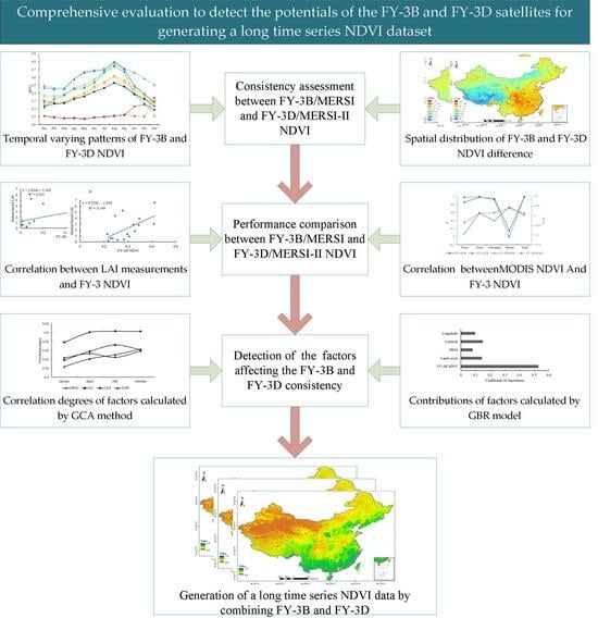
Comprehensive Assessment of NDVI Products Derived from Fengyun Satellites across China

Abstract

NDVI data are crucial for agricultural and environmental research. The Fengyun-3 (FY-3) series satellites are recognized as primary sources for retrieving NDVI products on a global scale. To apply FY-3 NDVI data for long-term studies, such as climate change, this study conducted a thorough evaluation to detect the potentials of the FY-3B and FY-3D satellites for generating a long time series NDVI dataset. For this purpose, the spatiotemporal consistency between the FY-3B and FY-3D satellites was evaluated, and their performances were compared. Then, a grey relational analysis (GRA) method was applied to detect the factors influencing the consistency among the different satellites, and a gradient boosting regression (GBR) model was constructed to create a long-term FY-3 NDVI product. The results indicate an overall high consistency between the FY-3B and FY-3D NDVIs, suggesting that they could be used as complementary datasets for generating a long-term NDVI dataset. The correlations between the FY-3D NDVI and the MODIS NDVI, as well as the leaf area index (LAI) measurements, were both higher than those of FY-3B, which indicates a better performance of FY-3D in retrieving NDVI data. The grey correlation degrees between the NDVI differences and four parameters, which were land cover (LC), DEM, latitude (LAT) and longitude (LON), were calculated, revealing that the LC was the most related to the NDVI differences. Finally, a GBR model with FY-3B NDVI, LC, DEM, LAT and LON as the input variables and FY-3D NDVI as the target variable was established and achieved a robust performance. The R values between the GBR-estimated NDVI and FY-3D NDVI reached 0.947, 0.867 and 0.829 in the training, testing and validation datasets, respectively, indicating the feasibility of the established model for generating long time series NDVI data by combining data from the FY-3B and FY-3D satellites.

1. Introduction

Vegetation coverage and growth conditions are crucial information for estimating global carbon sequestration, investigating vegetation–climate interactions and managing natural resources [1,2,3]. Over the past decades, a large number of remote sensing vegetation indicators, such as the enhanced vegetation index (EVI), normalized difference vegetation index (NDVI), fractional vegetation cover (FVC) and leaf area index (LAI), have been developed for mapping vegetation dynamics on a regional scale. As one of the most important and useful vegetation parameters, the remote-sensed NDVI has been extensively adopted for forecasting agricultural production, detecting drought intensities and exploring the climate effects on vegetation conditions in many previous studies [4,5,6]. In general, NDVI products can be derived from surface reflectance in the near-infrared and red wavelengths through several primary sensors, including the advanced very high resolution radiometer (AVHRR) on board the National Oceanic and Atmospheric Administration (NOAA) satellites, the moderate resolution imaging spectroradiometer (MODIS) on board Terra and Aqua, the enhanced thematic mapper plus (ETM+) on board Landsat, the medium resolution spectral imager (MERSI) and the second-generation MERSI (MERSI-II) on board the Fengyun-3 (FY-3) series satellites [7,8,9,10].

The FY-3 series satellites, including the FY-3A, FY-3B, FY-3C, FY-3D, FY-3E, FY-3G, FY-3F and additional satellites to be launched in the next few years, are China’s second-generation polar-orbiting meteorological satellites. These satellites are equipped with more than ten sets of advanced remote sensing instruments, such as the visible and infrared radiometer (VIRR), global navigation occultation sounder (GNOS), microwave radiometric imager (MWRI), high spectral infrared atmospheric Sounder (HIRAS), microwave temperature sounder (MWTS) and microwave humidity sounder (MWHS), thus enabling them to collect the quantitative, multispectral, three-dimensional and all-weather earth surface characteristic parameters on a global scale [11,12]. Among these instruments, the MERSI and MERSI-II sensors were designed as key visible and infrared spectral imaging instruments for detecting the atmospheric, terrestrial and oceanic features, and providing important operational products such as the outgoing longwave radiation (OLR), precipitable water vapor (PWV) and NDVI. Compared to MERSI onboard FY-3A/B/C satellites, the performance of MERSI-II onboard FY-3D has been greatly upgraded and improved, with more imaging channels, a higher radiometric calibration accuracy and an enhanced infrared detection capability [12]. In many previous studies, FY-3 MERSI and MERSI-II data have been widely used to monitor the vegetation coverage and conditions, detect natural disaster events and support weather forecasting sand environmental studies [13,14,15,16].

Cross-comparisons among vegetation indices (VIs) derived from different satellites and sensors is of great significance for their application, calibration and cooperative inversion using multisource remote sensing data [11]. Many previous studies have utilized methods such as regression analysis to recognize differences between VIs extracted from different satellite systems and sensors [17,18,19]. For example, seven VIs, including NDVI, EVI, normalized difference water index (NDWI), soil adjusted vegetation index (SAVI), green vegetation index (GVI), land surface water index (LSWI) and normalized burn ratio (NBR), provided by two sensors, which are the ETM+ on board Landsat 7 and the operational land imager (OLI) on board Landsat 8, were compared by researchers. The results showed that the correlation coefficients between different indices from ETM+ and OLI were high, indicating that those two sensors can be used to collect complementary data [17]. Additionally, the NDVI values across different land cover types from Landsat 7 and Landsat 8 were compared, revealing that differences between NDVI images from the two satellites were larger in low-vegetation-covered areas than in high-vegetation-covered areas, which indicates the need for calibration in low-vegetation-covered areas to achieve higher consistency between Landsat 7 and Landsat 8 NDVI images [20]. Despite the large number of early studies regarding cross-comparison analyses between vegetation parameters from different sensors and satellites, few studies have focused on the NDVI product from different generations of the FY-3 series satellites.

The FY-3D satellite equipped with the upgraded MERSI-II instrument was launched in November 2017 and started to provide an operational NDVI product in 2019, which indicates the short time series of the FY-3D NDVI data. Thus, the application of FY-3D NDVI in fields such as climate change was limited.

To solve this issue, this work proposes a novel scheme, as follows: Firstly, the consistency between FY-3B and FY-3D NDVI data was assessed to detect the possibility of combining different FY-3 satellites’ data into complementary datasets for generating a long-term NDVI dataset. Secondly, a correlation analysis between FY-3 products and two reference datasets was conducted to determine the satellite with the better performance. Thirdly, a grey correlation method was applied to detect the possible factors that could affect the consistency degree among different satellites. Finally, an ensemble regression model was established for generating long time series NDVI data by combining different FY-3 satellites. The paper is organized as follows: Section 2 introduces the study area, data, and methods. In Section 3, the results are described. Section 4, Section 5 and Section 6 illustrate the discussion, practical applications and conclusions, respectively.

2. Data and Methods

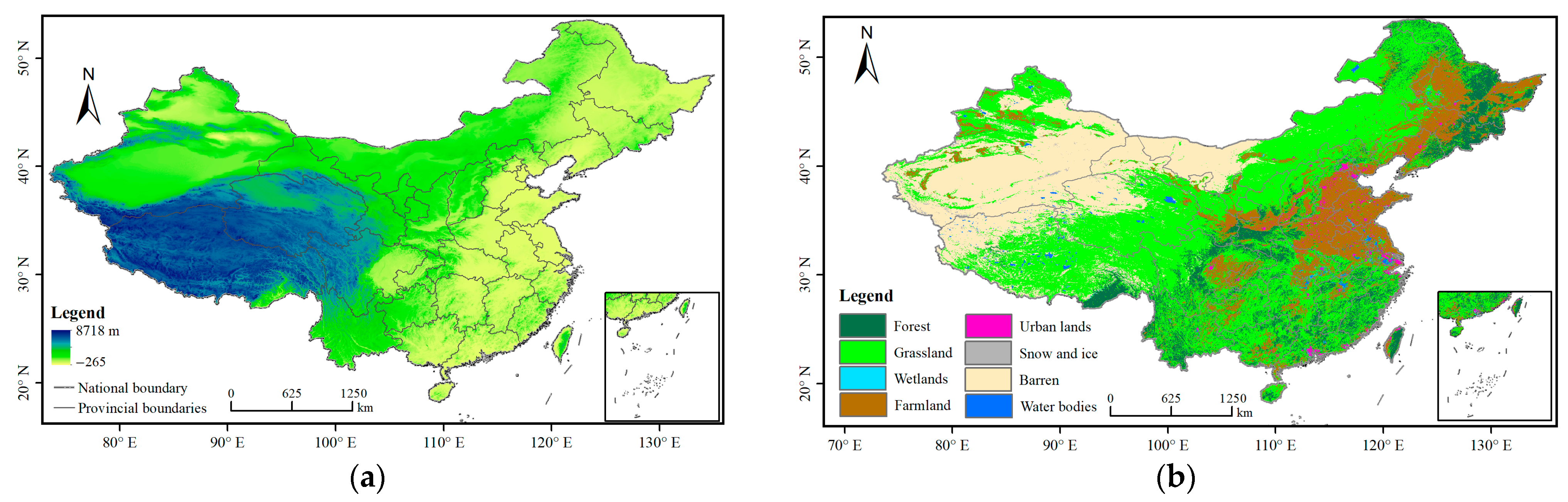
2.1. Study Area

China is the world’s third largest country with an approximately 9.6 million km² territory area. It is located in the east of Asia and on the west coast of the Pacific Ocean with coordinates of 18°N to 54°N and 73°E to 135°E (Figure 1). The terrain of China gradually increases from lower than 100 m in the east to more than 8000 m in the west. The Qinghai Tibet Plateau, known as the roof of the world, is located in the southwest of the study area, with an average elevation of 4000 m (Figure 1a). There are mainly six land cover types across China, including forest, grassland, farmland, barren, urban lands and water bodies, as shown in Figure 1b. Most parts of China are covered by various vegetation types. The forests are mainly distributed in southeastern and northeastern China, showing a regular zonal distribution from north to south. Grasslands are widely distributed in the northwestern, southeastern and northeastern regions of the study area. The distribution of farmland in China is quite unbalanced due to the effects of topography and climate environments, especially the water resources. Most cultivated lands are densely located in the central and eastern regions with flat terrain, mild climate and abundant precipitation.

Over the past several decades, China has experienced a rapid increase in extreme climate event occurrences in the context of global climate change, which have led to spatio-temporal changes in vegetation coverage and other vegetation activities [21,22]. Therefore, it is urgent and of great importance to achieve accurate and continuous NDVI dataset on a regional scale for China’s vegetation monitoring and carbon sequestration detection.

2.2. Data

2.2.1. RCH-CEOS NDVI Product Derived from Fengyun Satellites

To produce a highly homogenous and long time series NDVI product for vegetation applications in fields such as climate change, the National Satellite Meteorological Center (NSMC) adopted the unified calibration method to achieve the Retrospective Calibration of Historical Chinese Earth Observation Satellites (RCH-CEOS) NDVI dataset. The RCH-CEOS NDVI product was derived from the calibrated Level 1 reflectance of FY-3A, FY-3B MERSI and FY-3D MERSI-II, with spatial resolutions of 1 km and 250 m. The maximum value composite (MVC) approach was applied to generate the composite NDVI maps from 2010 to 2023 at ten-day and monthly intervals [10,23]. Among them, the NDVI products for 2010, 2011–2020 and 2019–2023 were derived from the FY-3A, FY-3B and FY-3D satellites, respectively. In this study, pixel values were extracted from FY-3B/MERSI and FY-3D/MERSI-II NDVI products for the months from January to December 2020. The averaged NDVI values for forest, grassland, farmland, barren land and the entire country were then calculated and compared to assess the consistency among the RCH-CEOS NDVI products derived from different Fengyun satellites.

2.2.2. In Situ LAI Measurements from CMA

The website for the China meteorological data (https://data.cma.cn/, accessed on 18 October 2023), which is operated by the National Meteorological Information Center (NMIC) of the China Meteorological Administration (CMA), collects and releases an abundance of weather-related data, including meteorological station-based measurements, radar and satellite remote sensing images, numerical forecasting products, reanalysis data, atmospheric composition data and climate forecasting products. Here, 16 in situ LAI measurements collected from agrometeorological stations were downloaded from the China meteorological data website, and the latitudes and longitudes of each station were applied to calculate the rows and columns of station pixels located at the FY-3 NDVI images. Then the correlation between NDVI values at those pixels and the LAI measurements was analyzed to identify the ability of FY-3B and FY-3D for monitoring the vegetation growth on a site scale.

2.2.3. Land Cover and NDVI Products Derived from MODIS

The MODIS acquires the features of the land, ocean and atmosphere every 1–2 days and provides important time series datasets for quantifying changes in the global environment [24]. Many of the MODIS’s data and products, such as the MODIS land cover (MODIS LC) and MODIS NDVI products, have been widely used for land cover type classification and crop yield estimation in many early studies [25,26]. The MODIS LC products (MOD12Q1) contain 17 land cover types based on the international geosphere biosphere programme (IGBP) scheme. Here, these land cover types were merged into 8 types, including forest, grassland, wetland, farmland, urban and built-up land, barren, snow and ice, and water bodies, for assessing the consistency among NDVI values of FY-3 satellites across various land types. The MODIS NDVI products (MOD13A3, v006) for the months from January to December 2020 were downloaded from the NASA website (https://ladsweb.modaps.eosdis.nasa.gov/, accessed on 11 October 2023) as the reference dataset. Then, the correlation coefficients between MODIS NDVI and NDVI values derived from the different FY-3 satellites were calculated to evaluate the ability of FY-3B and FY-3D for monitoring vegetation conditions on a regional scale.

2.2.4. DEM Data from GMTED2010

The digital elevation model (DEM) is one of the branches of the digital terrain model (DTM), which is a discrete mathematical representation of the Earth’s surface topography, and is frequently selected as auxiliary data for use in many areas of research [27,28]. The global multiresolution terrain elevation data in the 2010 (GMTED2010) dataset contain multisource elevation data, including shuttle radar topography mission (SRTM) digital terrain elevation data from US National Geospatial-Intelligence Agency (NGR), Canadian digital elevation data, US continental and Alaska elevation data, the second DEM for Australia and the DEM from Antarctic and Greenland radar and laser altimeters [29]. The GMTED2010 dataset has proven to be more accurate than the GTOPO30 model and was adopted to map the topography across the study area in this study.

2.3. Methods

2.3.1. Grey Relational Analysis Method

The grey relational analysis (GRA) method, which is an important part of the theory of grey systems, has been extensively applied in conducting relational analyses, performing predictions, and solving decision-making problems in various sectors [30,31]. In general, the degree of similarity or diversity of the developing trend among factors are measured using the GRA method for achieving the relevance of multiple factors and ranking the alternatives [32,33,34].

The GRA method involves the following steps: Step 1: Define the reference sequence (X*) and m comparison sequences (Xⁱ) (i = 1, 2, …, m) as:

$$X^{*}=[{X_1}^{*},{X_2}^{*},\dots ,{X_k}^{*},\dots ,{X_n}^{*}]$$

(1)

$$X^i=[{X_1}^i,{X_2}^i,\dots ,{X_k}^i,\dots ,{X_n}^i]$$

(2)

where n is the number of samples in each sequence, k (k = 1, 2, …, n) is the index of samples, X_k* represents the reference sequence for the kth sample, and X_kⁱ represents the comparison sequence for the kth sample of the ith alternative. Step 2: Transform the original data into nondimensional sequences (C_kⁱ) ranging from 0 to 1 using the following equations:

$${C_k}^{*}=\frac{{X_k}^{*}-{X_{\min }}^{*}}{{X_{\max }}^{*}-{X_{\min }}^{*}}$$

(3)

$${C_k}^j=\frac{{X_k}^j-{X_{\min }}^j}{{X_{\max }}^j-{X_{\min }}^j}$$

(4)

where X_min* and X_max* are the minimum and maximum values for the reference sequence, respectively. X_min^j and X_max^j are the minimum and maximum values for the jth comparison sequence, respectively. Step 3: Calculate the grey relational coefficient (ξ_i^k) and grey relational degree (D_i) using the following equations:

$${{\xi }_i}^k=\frac{\underset{1\le i\le m}{\min }\underset{1\le k\le n}{\min }\left|{C_k}^{*}-{C_k}^i\right|+\rho \underset{1\le i\le m}{\max }\underset{1\le k\le n}{\max }\left|{C_k}^{*}-{C_k}^i\right|}{\left|{C_k}^{*}-{C_k}^i\right|+\rho \underset{1\le i\le m}{\max }\underset{1\le k\le n}{\max }\left|{C_k}^{*}-{C_k}^i\right|}$$

(5)

$$D_i=\frac{1}{n}{\displaystyle \sum }_{k=1}^n{{\xi }_i}^k$$

(6)

where ρ is the identification coefficient ranging from 0 to 1, which was set as ρ = 0.5 in this study. ξ_i^k represents the grey relational coefficient between C_kⁱ and C_k*. D_i represents the grey relational degree between the reference sequence and the ith comparison sequence. A greater value of D_i indicates a higher proximity of sequence Xⁱ to the reference sequence [35].

In this study, the GRA method was adopted to analyze the importance of factors influencing the NDVI bias from different Fengyun satellites. Here, the difference between the FY-3B and FY-3D NDVI values in 2020 was set as the reference sequence, and several potential influencing factors, such as the land cover types, during the same period were set as the sequences to be compared. Then, the grey relational degrees between the reference and comparison sequences were calculated to rank the importance of each factor influencing the NDVI difference.

2.3.2. Gradient Boosting Regression Model

Various versions of the boosting algorithm, such as AdaBoost and gradient boosting (GB), have proven to be very competitive in a wide range of applications [36,37]. Among them, the GB model, which was introduced by Friedman, in 2001, has been extensively applied for solving classification and regression problems as one of the most powerful ensemble learning techniques [38,39,40,41].

In general, the performance of the GB model is improved by training a series of basic learners and minimizing the expectations of the loss function [41]. There are several most frequently used loss functions, including the Gaussian L2 loss function, Laplace L1 loss function, Huber loss function and Quantile loss function [39]. Here, the Huber loss function was selected considering its robustness to outliers. The Huber loss function comprises two parts and is designed as follows:

$${L(y,f(x))}_{Huber,\delta }=\left\{\begin{array}{l}{(y-f(x))}^2/2\hspace{1em}\hspace{1em}\hspace{1em}\left|y-f(x)\right|\le \delta \\ \delta (\left|y-f(x)\right|-\delta /2)\hspace{1em} \left|y-f(x)\right|>\delta \end{array}\right.$$

(7)

where y is the true value, f(x) is the predicted value and δ is the threshold parameter, which specifies the robustness of the Huber loss function. To achieve a more accurate global optimum and reduce the time needed to update those parameters, the mean squared error (MSE) is applied when the prediction error is less than or equal to δ, and a linear error indicator such as mean absolute error (MAE) is applied when the prediction error is greater than δ.

The GB model is built in a stepwise fashion. For each step, the pseudo-residual of each weak learner decreases in the direction of the negative gradient by fitting the negative gradient of the loss function of the previously cumulative model, so that the cumulative model loss decreases after the addition of the weak learner. Assume that the number of training samples is n. The approximate solution is initialized as:

$$F_0(x)=\arg {\min }_{f\in F}{\displaystyle \sum _{i=1}^{m}L(y_i,f(x_i))}$$

(8)

where f is one of the basic learners, and F is the set of basic learners.

Assume that the number of applied basic learners is m. For step j (j = 1, 2, …, m), the negative gradient G and learner f for the current step are computed as follows:

$$G_j(x_i)={\left[-\frac{\partial L(y_i,f(x_i))}{\partial f(x_i)}\right]}_{f(x_i)=f_{j-1}(x_i)}$$

(9)

$$f_j(x_i)={\nu }_j{G}_j(x_i)$$

(10)

where the parameter ν is the multiplier and is computed based on the following equation:

$${\nu }_j=\arg {\min }_{\rho }{\displaystyle \sum _{i=1}^{n}L(y_i,f(x_i)+{\nu }_j{G}_j(x_i)})$$

(11)

Then, the GB model is updated as follows:

$$F_j(x_i)=F_{j-1}(x_i)+f_j$$

(12)

In this study, to further improve the consistency among the NDVI products derived from different Fengyun satellites, the gradient boosting regression (GBR) model was built for the NDVI estimations, pixel by pixel, using multiple inputs.

2.4. Evaluation Criteria

To evaluate the consistency between the FY-3D NDVI product and the NDVI derived from FY-3B and the estimated NDVI using the multivariate GBR model, five statistical indicators, including the correlation coefficient (R), root mean square error (RMSE), mean absolute error (MAE) and rate of change (RoC), were adopted in this study.

The R represents the relative accuracy between the original FY-3B NDVI retrievals or the estimated NDVI values using the GBR model and the FY-3D NDVI retrievals, respectively, and can be defined by Equation (13).

$$\mathrm{R}=\frac{{\displaystyle {\sum }_{i-1}^N(CNDV{I}_i-\overline{CNDVI})(RNDV{I}_i-\overline{RNDVI})}}{\sqrt{{\displaystyle {\sum }_{i-1}^N{(CNDV{I}_i-\overline{CNDVI})}^2}\sqrt{{\displaystyle {\sum }_{i-1}^N{(RNDV{I}_i-\overline{RNDVI})}^2}}}}$$

(13)

where CNDVI_i represents the NDVI values to be compared, which refer to the FY-3B NDVI and the GBR-estimated NDVI values in this study. RNDVI_i represents the reference NDVI values, i.e., the FY-3D NDVI retrievals. $\overline{\mathit{CNDVI}}$ represents the average of the FY-3B NDVI retrievals or the GBR NDVI estimations across all pixels in the study area, $\overline{\mathit{RNDVI}}$ indicates the average of the FY-3D NDVI retrievals, and N represents the number of valid pixels in each dataset.

The RMSE and MAE evaluate the absolute difference between the FY-3B NDVI product or NDVI estimations using the GBR model and the FY-3D NDVI data, which can be calculated by Equations (14) and (15).

$$\mathrm{RMSE}=\sqrt{\frac{{\displaystyle {\sum }_{i=1}^N{(CNDV{I}_i-RNDV{I}_i)}^2}}{N}}$$

(14)

$$\mathrm{MAE}=\frac{1}{N}{\displaystyle {\sum }_{i-1}^N\left|CNDV{I}_i-RNDV{I}_i\right|}$$

(15)

The RoC evaluates the degree of the GBR model for improving the consistency between NDVI products from FY-3B and FY-3D, and it can be defined as the following equation:

$$\mathrm{RoC}=\frac{E_g-E_b}{E_b}\times 100\%$$

(16)

where E_g represents the error metrics between the GBR-estimated NDVI and the FY-3D NDVI data, and E_b represents the error metrics between the FY-3B NDVI and the FY-3D NDVI data.

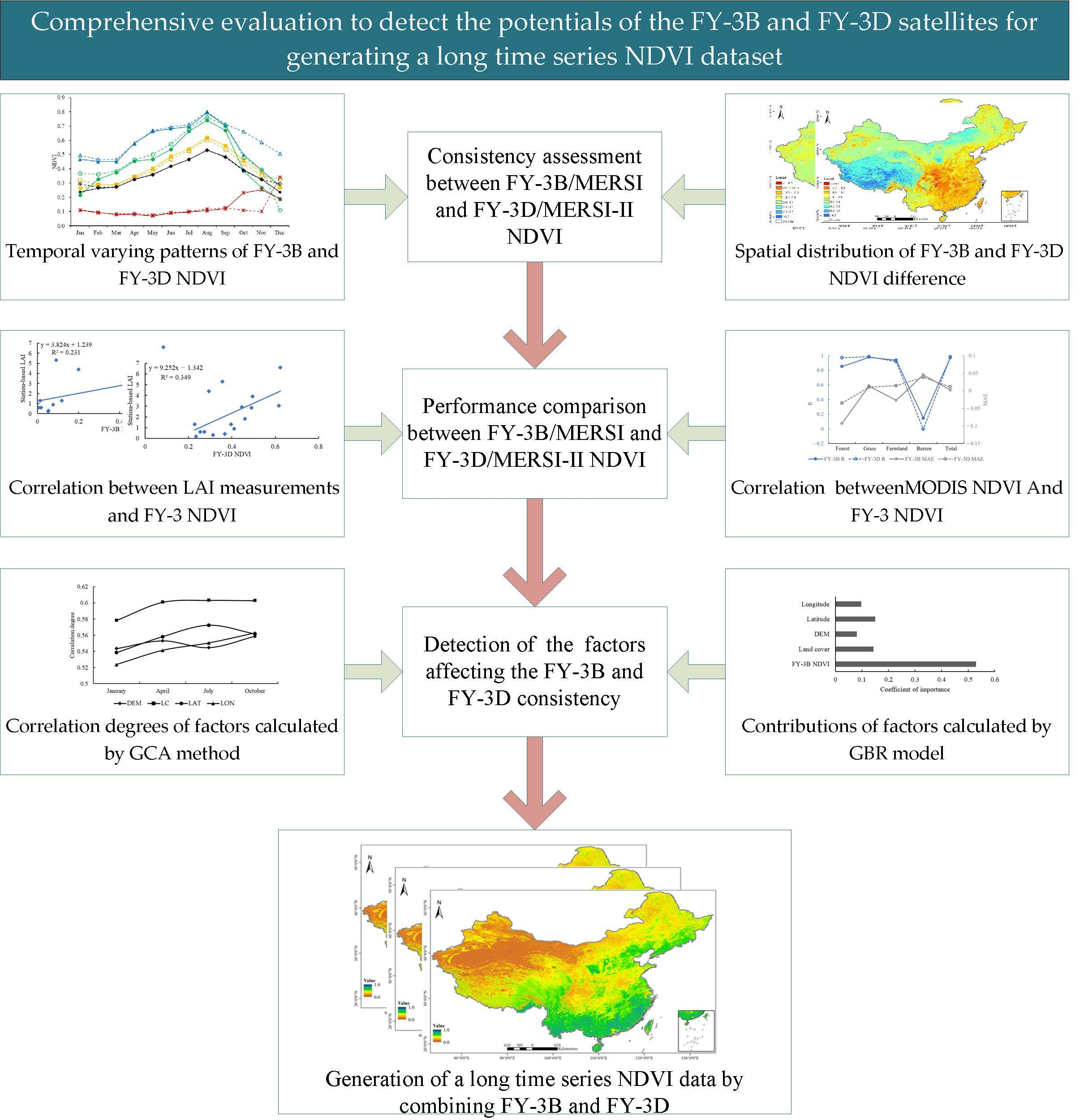
3. Results and Analysis

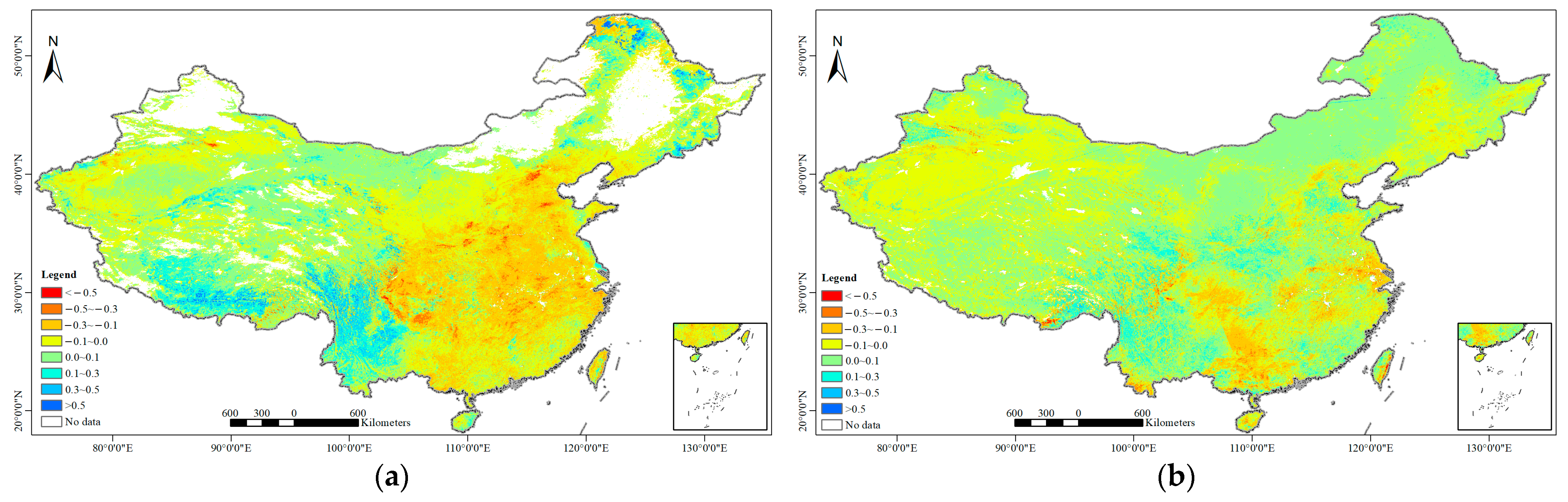
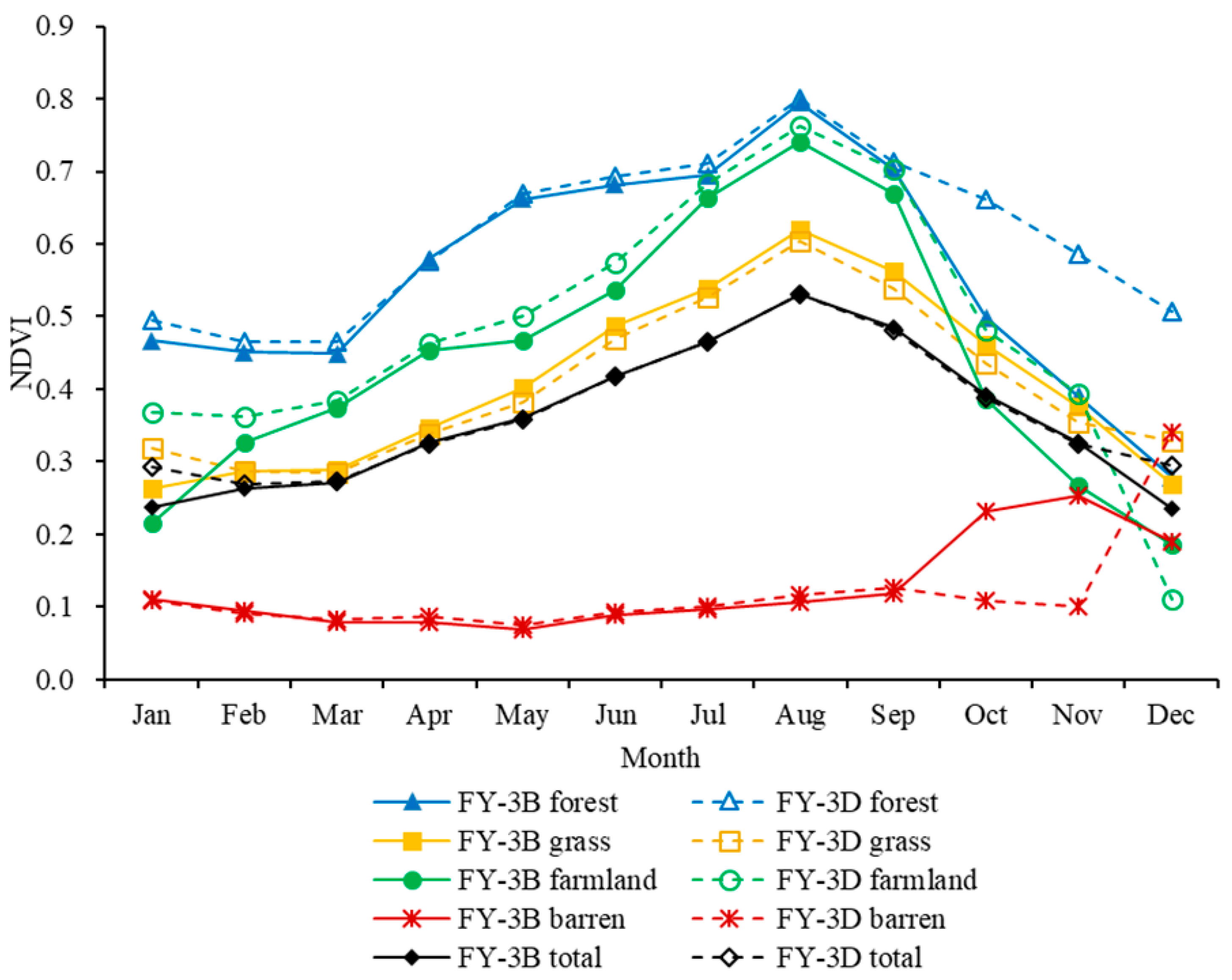
3.1. Consistency Assessment of NDVI Products Derived from Different Fengyun Satellites

The variation curves of FY-3B NDVI (solid line) and FY-3D NDVI (dash line) for different land cover types in 2020 are displayed in Figure 2. Generally, the FY-3B and FY-3D NDVI data showed an overall high consistency, with the averaging NDVI difference values across the study area being lower than 0.01. However, the NDVI differences varied in different time periods and for different land cover types. In particular, the deviations between FY-3B and FY-3D from October to December were larger than in other months. For the forest and farmland areas, the NDVI value of FY-3D was slightly higher than that of FY-3B. The FY-3D NDVI was slightly lower than FY-3B NDVI in most months for the grassland.

The spatial distributions of the NDVI difference values between FY-3B and FY-3D in January, April, July, and October 2020 are mapped in Figure 3. Generally, the FY-3B NDVI values in the southeast region of the study area were lower than those of FY-3D, and the FY-3B NDVI values in southwest China were greater than those of FY-3D. The NDVI differences vary in different months. Compared with April and July, the FY-3B and FY-3D NDVIs’ difference in January and October was significantly higher.

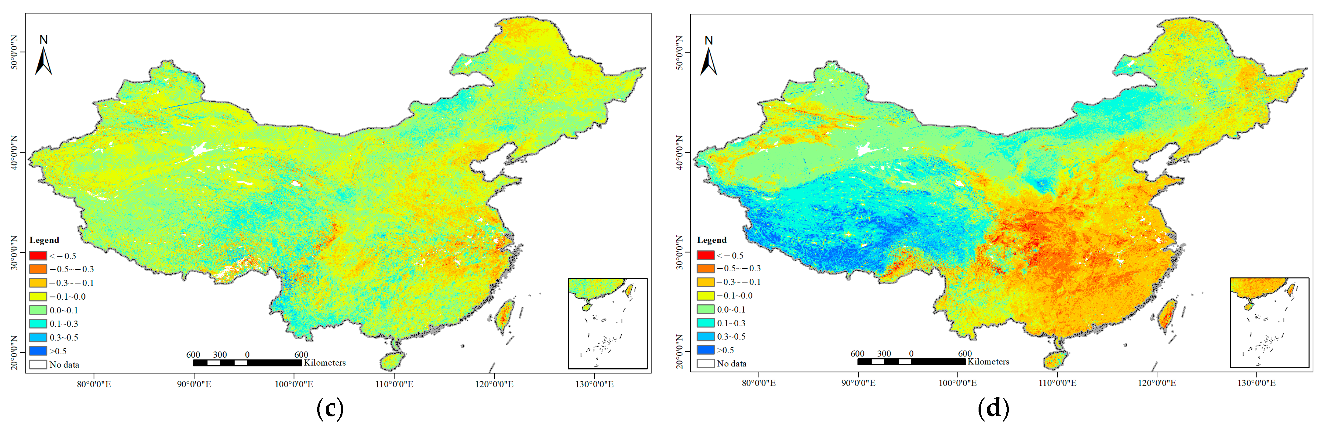
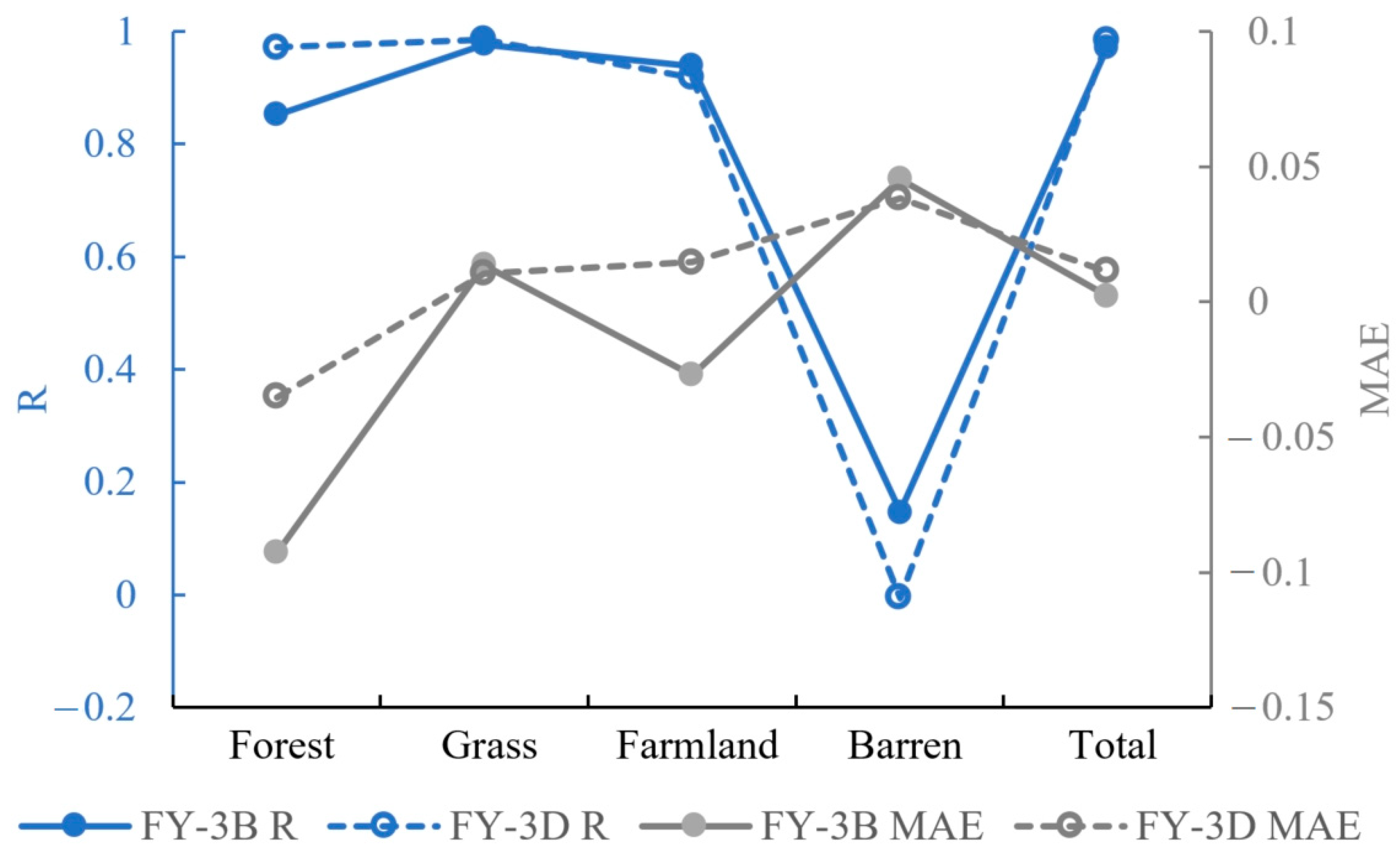
3.2. Comparing the Performances of Different Fengyun Satellites in Monitoring Vegetation Conditions

To further evaluate the potentials of the FY-3B and FY-3D NDVIs for monitoring vegetation growth conditions, a correlation analysis between the measured LAI data and the NDVI values extracted from the FY-3B and FY-3D satellites was conducted. The scatterplots and the coefficients of determination (R²) are shown as Figure 4. The results show that the R² value between the FY-3D NDVI and the station-based LAI (0.349) was higher than that between the FY-3B NDVI and the in situ LAI measurements (0.231), which indicates that the FY-3D NDVI is more reliable in reflecting vegetation growth and conditions on a site scale.

The MODIS NDVI is recognized as one of the most popular vegetation indices; thus, it was selected to evaluate the abilities of FY-3B and FY-3D for monitoring vegetation conditions on a grid scale. The R and MAE values between MODIS NDVI and NDVI products extracted from the FY-3B and FY-3D satellites were calculated, as shown in Figure 5. The results show that the R value between the MODIS NDVI and the NDVI values calculated by FY-3D and FY-3B across all pixels in the study area reached 0.983 and 0.973, respectively, indicating that the overall consistency between the MODIS NDVI and the FY-3D NDVI was slightly higher than that of the FY-3B NDVI. In addition, the averaged MAE values of FY-3B and FY-3D were both less than 0.01, indicating that the FY-3 NDVI and the MODIS NDVI were generally close.

The consistency between the FY-3 and MODIS NDVI varied for the different land cover types. The FY-3 NDVI and MODIS NDVI for grassland achieved the highest consistency, with R values between the MODIS NDVI and the NDVI derived from FY-3B and FY-3D, reaching 0.976 and 0.985, and the MAE values reached 0.013 and 0.010, respectively. The FY-3B and FY-3D NDVI values for forest were lower than that of the MODIS NDVI, and the underestimation degree of FY-3B (MAE = −0.092) was higher than that of FY-3D (MAE = −0.035). For farmland, the FY-3B NDVI was lower than the MODIS NDVI, with an MAE value equivalent to −0.027, while the FY-3D NDVI was much closer to the MODIS NDVI with an MAE value equivalent to 0.014. Among those land cover types, the correlations with barren areas were the worst, with average R values lower than 0.2.

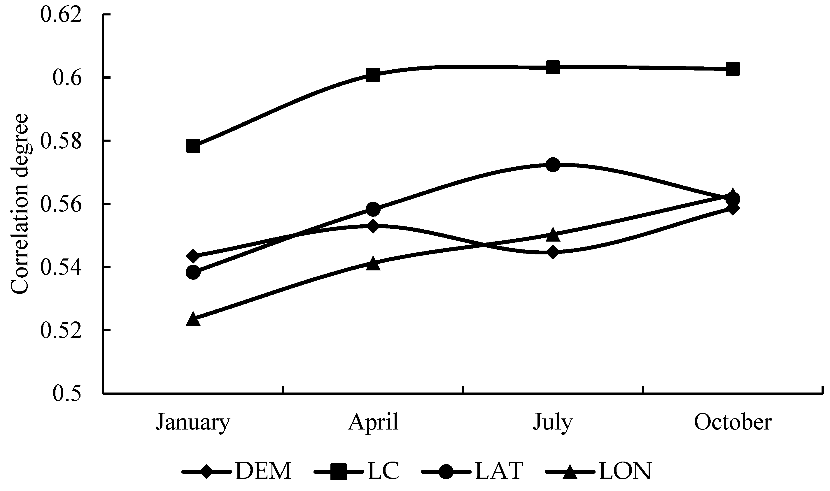
3.3. Detecting the Factors Affecting the NDVI Difference Using the GRA Method

In this study, the GRA method was applied to analyze the factors affecting the NDVI difference in January, April, July and October. Firstly, the FY-3B and FY-3D NDVIs’ difference values at each pixel were extracted to construct the reference sequence. The DEM, LC, LAT and LON values at pixels were used to construct four sequences to be compared. Then, the correlation degree values between the reference sequence and those comparison sequences were calculated according to Equations (3)–(6), as shown in Figure 6. The grey correlation between the NDVI difference sequence and the LC sequence was the highest in each month, with correlation degree values reaching 0.578, 0.601, 0.603 and 0.603 in January, April, July and October, respectively, which illustrated that the land cover condition was closely related to the FY-3B and FY-3D NDVIs’ difference. By ranking the grey correlation degrees in decreasing order, the importance of those affecting factors were ranked as follows: LC > DEM > LAT > LON in January; LC > LAT > DEM > LON in April; LC > LAT > LON > DEM in July; and LC > LON > LAT > DEM in October.

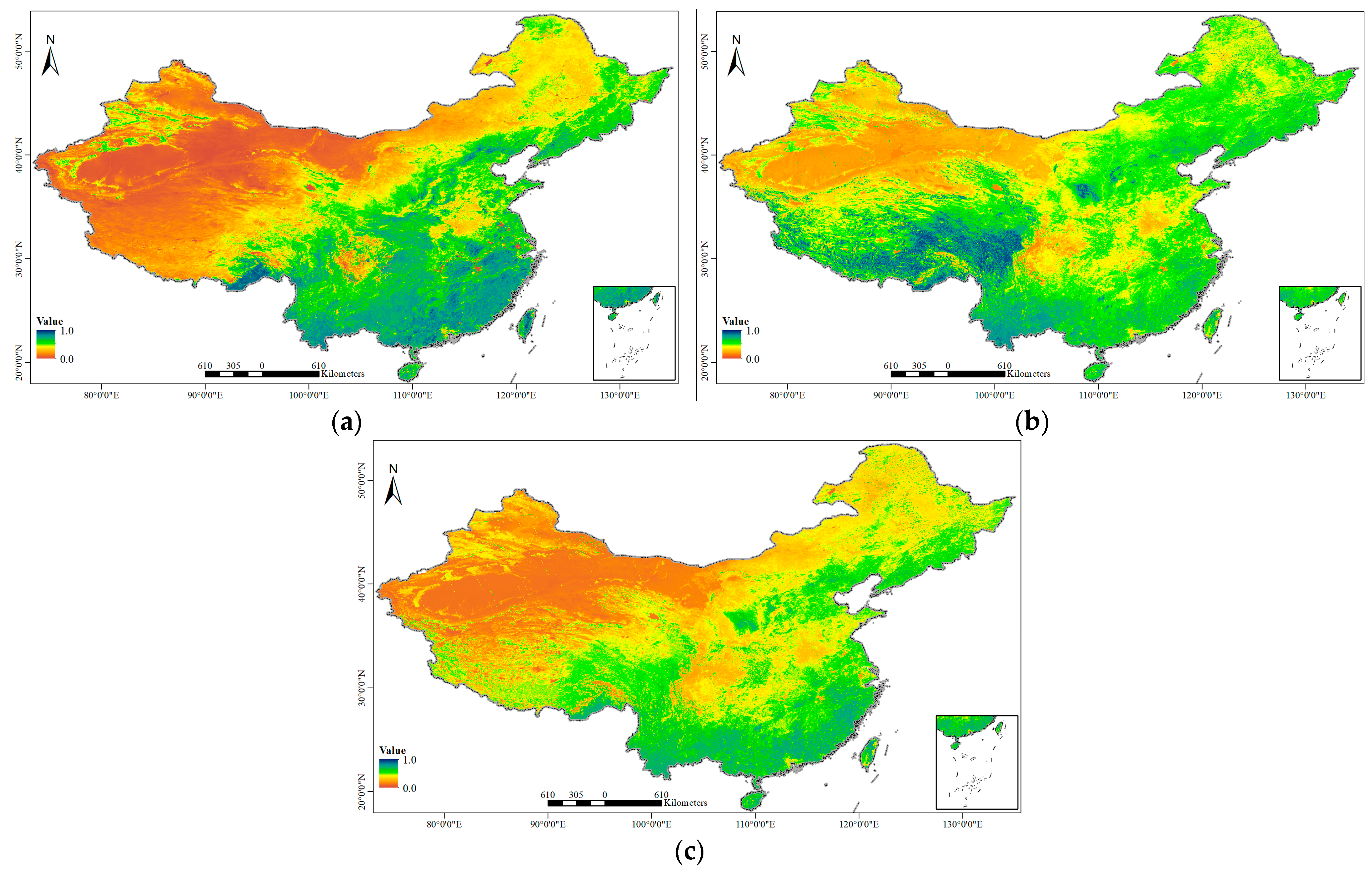
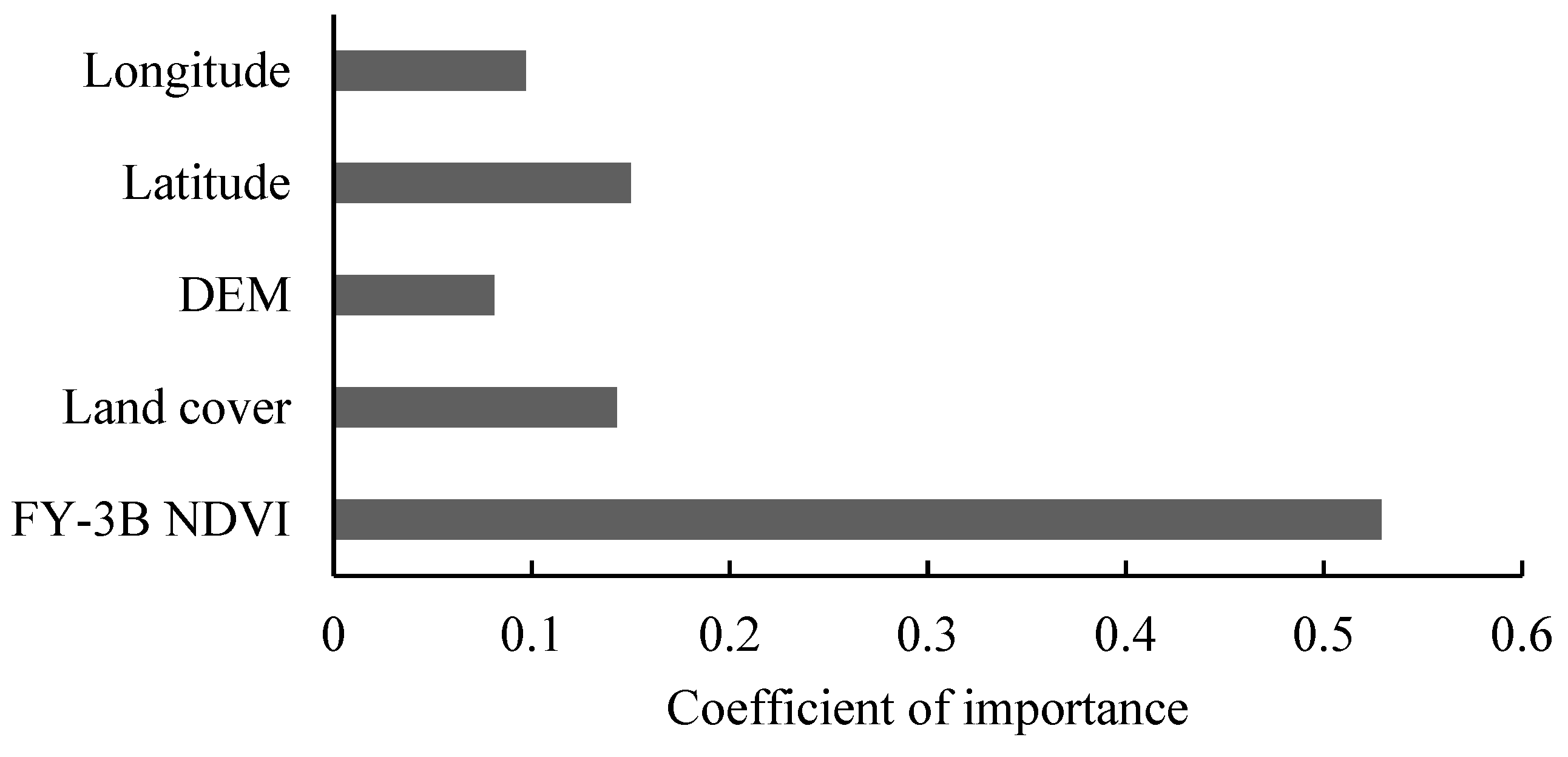
3.4. Establishing a GBR Model for Forming Long Time Series NDVI Data

In this study, the monthly FY-3B and FY-3D NDVI products in 2019 and 2020, as well as several auxiliary data, including the DEM, LC, LAT and LON, were selected to establish and validate the GBR model for improving the consistency among NDVI products extracted from different FY-3 satellites. To be specific, 90% and 10% of the samples in 2019 were adopted as the training and testing datasets, respectively, and the samples in 2020 were used as the validation dataset. Considering that the inconsistency issue was relatively more serious in October, as demonstrated in Section 3.1, a GBR model with the FY-3B NDVI, LC, DEM, LAT and LON as the input variables and FY-3D NDVI as the target variable was built to correct the FY-3B NDVI for the formation of a long-term FY-3 NDVI product in October.

The error metrics, including R, RMSE, MAE and RoC, between the reference variable (FY-3D NDVI) and the NDVI values extracted from the FY-3B satellite, as well as the estimated NDVI using the GBR model (GBR NDVI), were calculated as shown in

Table 1. The error metrics between the FY-3D NDVI retrievals and the NDVI values extracted from the FY-3B and the GBR model.

	Error	FY-3B NDVI				GBR NDVI
Dataset		R	p	RMSE	MAE	R	p	RoC	RMSE	RoC	MAE	RoC
Training		0.902	<0.001	0.092	0.065	0.947	<0.001	+5.0%	0.067	−27.2%	0.046	−29.2%
Testing		0.774	<0.001	0.120	0.090	0.867	<0.001	+17.2%	0.101	−15.8%	0.078	−13.3%
Validation		0.547	<0.001	0.213	0.159	0.829	<0.001	+51.6%	0.140	−34.3%	0.107	−32.7%

. The results showed that the R values between the GBR NDVI and FY-3D NDVI reached 0.947, 0.867 and 0.829 in the training, testing and validation datasets, respectively, which greatly increased by 5.0%, 17.2% and 51.6% compared with that between the FY-3B and FY-3D NDVIs. In addition, the RMSE values decreased by 27.2%, 15.8% and 34.3%, and the MAE values decreased by 29.2%, 13.3% and 32.7% during the training, testing and validation processes, respectively, which indicated a robust performance of the GBR for generating long time series NDVI data by combining data from the FY-3B and FY-3D satellites.

The importance coefficients of each input factor were calculated by the GBR model and are shown in Figure 7. Among those variables, the FY-3B NDVI contributed the most, with the coefficient of importance (CI) reaching 0.529, followed by the latitude (CI = 0.150) and land cover (CI = 0.143). The longitude and DEM contributed less than the other variables, with the CI values equivalent to 0.097 and 0.081, respectively.

The established GBR model was applied to perform the NDVI estimations across the study area, pixel by pixel. The FY-3D, FY-3B and GBR model-based NDVI images were mapped and are displayed in Figure 8. Compared to the FY-3D NDVI (Figure 8a), the FY-3B NDVI (Figure 8b) significantly overestimated the NDVI values in the southwest (mainly the Qinghai–Tibet Plateau) and northeast parts of the study area. The overestimation issue was largely improved in the estimated NDVI product based on the GBR model (Figure 8c), which indicates the feasibility of the use of the established GBR model for generating long time series Fengyun NDVI data with higher consistency.

4. Discussion

A large number of China’s Fengyun meteorological satellites were launched in recent years to support weather forecasting and extreme events detection. However, the products derived from the Fengyun satellites are limited for long-term applications in fields such as climate change due to their short time series. This study explored the possibility of generating a long-term NDVI dataset by combining different Fengyun satellite NDVI products. The results are promising and can be used as a reference idea and method for evaluating and improving Chinese Fengyun satellite products for weather and climate applications.

Previous studies have pointed out that the observed NDVI signal could be greatly affected by the aerosol optical depth (AOD), which could significantly underestimate the amount of vegetation [42,43]. Apart from the AOD, atmospheric water vapor, clouds, and differences in spectral wavelengths could also cause differences in NDVI values [44,45]. The results in this work have shown a relatively lower consistency between the FY-3B and FY-3D NDVIs during the months from October to December than in other months. This can be attributed to the relatively higher aerosol loads in winter, as well as the differences in spectral wavelengths of FY-3B/MERSI and FY-3D/MERSI-II. Compared with the MERSI, the number of MERSI-II channels increased from 20 to 25, with more infrared channels and enhanced infrared detection capability [23]. Moreover, the FY-3D NDVI applied the 6SV method for atmospheric correction and greatly decreased the atmospheric effects [10], thus achieving more accurate NDVI data in periods with higher aerosol optical thickness.

Field campaigns and ground truth could greatly contribute to the evaluation and validation processes of satellite remote sensing products [46]. In this study, the in situ LAI measurements were selected as reference data to evaluate and compare the capacity of the FY-3B and FY-3D for monitoring vegetation growth conditions because of the unavailability of ground-based NDVI or spectral measurements. The results indicate a higher correlation between the FY-3D and LAI measurements than that of the FY-3B, which could be explained by the fact that the FY-3D carries more advanced instruments than the FY-3B. Although a reasonable result was achieved, there are several issues with the current LAI data, which could cause a biased evaluation of the performance of remote sensing products. The in situ LAI data contain only two land cover types, which are grassland and farmland; thus, the representativeness of the LAI samples needs to be further improved in future studies for a more reliable evaluation. In additions, the mismatch of scales between meteorological stations and satellites could also potentially influence the reliability of the assessment [47].

5. Practical Applications

This work provides a reliable method for evaluating and correcting NDVI products derived from different Chinese meteorological satellites for forming long time series NDVI data. The generated FY-3 long-term NDVI dataset could contribute to research in fields such as climate change, ecological environment detection, crop growth monitoring, phenological extraction and carbon sequestration trend analysis. For example, long-term NDVI time series data, together with other climatic data, can be applied to detect the effect of extreme events on vegetation activities [21]. This information is quite crucial for local ecosystem conservation, especially in climate-sensitive regions. Apart from these potential application fields of long-term NDVI data, the idea proposed by this study could be adopted as a reference method to process various remote sensing products, such as the land surface temperature (LST), outgoing longwave radiation (OLR) and surface soil moisture (SSM), from different Fengyun satellites for weather and climate applications in the future.

6. Conclusions

This study introduced an overall strategy that could be extended for evaluating and improving the Chinese FY-3 meteorological satellite systems for long-term environmental research on a regional scale. There are four main components contained in this strategy: (1) consistency assessment among different satellites to provide information for supplementary dataset selection and further improvement; (2) performance comparison among different satellites to recognize the target data for the correction model; (3) correlation analysis to detect the factors affecting the differences among satellites; and (4) an ensemble machine learning model to form long time series data by combining different satellites.

In this study, the variation trends of the FY-3B/MERSI and FY-3D/MERSI-II NDVIs for different land cover types in 2020 were compared, and the results show an overall high consistency between the FY-3B and FY-3D NDVIs, indicating the potential of the FY-3 satellites for providing long-term NDVI datasets as complementary data sources. The correlations between the FY-3 NDVI and two reference data, which were the MODIS NDVI and in situ LAI measurements, were analyzed to determine the satellite with the better performance. The correlation coefficients indicate that FY-3D/MERSI-II has a better capacity for retrieving an NDVI product on both the regional and site scales. This study applied the GRA method to detect the factors related to the NDVI differences among different satellites. The results show that the grey correlation degree between the LC and the NDVI difference sequences was the highest in each month, implying that the LC is an important parameter for the FY-3 NDVI product correction.

This study established a GBR model with the FY-3B NDVI, LC, DEM and geographical locations as input variables and the FY-3D NDVI as the target variable to generate long-term NDVI data using the FY-3B and FY-3D satellites. The R values between the model-based NDVI estimates and the FY-3D NDVI reached 0.947, 0.867 and 0.829 in the training, testing and validation datasets, respectively, which significantly improved compared with the R values between the FY-3B and FY-3D. Therefore, the GBR model has the feasibility to correct the FY-3B NDVI for generating a long-term FY-3 NDVI dataset, with the historical data more consistent with the upgraded data. In addition, this study calculated the feature importance of the GBR model. The results showed that the FY-3B NDVI contributed the most (0.529) to the model, followed by LAT (0.150), LC (0.143), LON (0.097) and DEM (0.081). Note that although the GBR model is one of the most widely used ensemble machine learning models for solving classification and regression problems, it has some limitations, such as a high sensitivity to outliers and complex parameter optimization, which suggests that it will be necessary to further optimize the parameter analysis in future studies to minimize its drawbacks and increase its performance.

References

- Dai, X.; Yang, G.; Liu, D.; Wan, R. Vegetation Carbon Sequestration Mapping in Herbaceous Wetlands by Using a MODIS EVI Time-Series Data Set: A Case in Poyang Lake Wetland, China. Remote Sens. 2020, 12, 3000. [Google Scholar] [CrossRef]
- Zhang, X.; Cao, Q.; Chen, H.; Quan, Q.; Li, C.; Dong, J.; Chang, M.; Yan, S.; Liu, J. Effect of Vegetation Carryover and Climate Variability on the Seasonal Growth of Vegetation in the Upper and Middle Reaches of the Yellow River Basin. Remote Sens. 2022, 14, 5011. [Google Scholar] [CrossRef]
- Thackway, R.; Lee, A.; Donohue, R.; Keenan, R.; Wood, M. Vegetation information for improved natural resource management in Australia. Landsc. Urban Plan. 2007, 79, 127–136. [Google Scholar] [CrossRef]
- Becker-Reshef, I.; Vermote, E.; Lindeman, M.; Justice, C. A generalized regression-based model for forecasting winter wheat yields in Kansas and Ukraine using MODIS data. Remote Sens. Environ. 2010, 114, 1312–1323. [Google Scholar] [CrossRef]
- Khan, J.; Wang, P.; Xie, Y.; Wang, L.; Li, L. Mapping MODIS LST NDVI imagery for drought monitoring in Punjab Pakistan. IEEE Access 2018, 6, 19898–19911. [Google Scholar] [CrossRef]
- Bhuyan, U.; Zang, C.; Vicente-Serrano, S.M.; Menzel, A. Exploring Relationships among Tree-Ring Growth, Climate Variability, and Seasonal Leaf Activity on Varying Timescales and Spatial Resolutions. Remote Sens. 2017, 9, 526. [Google Scholar] [CrossRef]
- Xiao, Z.; Liang, S.; Tian, X.; Jia, K.; Yao, Y.; Jiang, B. Reconstruction of long-term temporally continuous NDVI and surface reflectance from AVHRR data. IEEE J. STARS 2017, 14, 5551–5568. [Google Scholar] [CrossRef]
- Jin, Z.; Xu, B. A Novel Compound Smoother-RMMEH to Reconstruct MODIS NDVI Time Series. IEEE Trans. Geosci. Remote Sens. 2013, 10, 942–946. [Google Scholar] [CrossRef]
- Ke, Y.; Im, J.; Lee, J.; Gong, H.; Ryu, Y. Characteristics of Landsat 8 OLI-derived NDVI by comparison with multiple satellite sensors and in-situ observations. Remote Sens. Environ. 2015, 164, 298–313. [Google Scholar] [CrossRef]
- Han, X.; Weng, F.; Han, Y.; Huang, H.; Li, S. Vegetation indices derived from Fengyun-3D MERSI-II data. In Proceedings of the IGARSS 2020—2020 IEEE International Geoscience and Remote Sensing Symposium, Waikoloa, HI, USA, 26 September–2 October 2020. [Google Scholar]
- Xiao, F.; Liu, Q.; Li, S.; Qin, Y.; Huang, D.; Wang, Y.; Wang, L. A Study of the Method for Retrieving the Vegetation Index from FY-3D MERSI-II Data. Remote Sens. 2023, 15, 491. [Google Scholar] [CrossRef]
- Yang, Z.D.; Zhang, P.; Gu, S.Y. Capability of Fengyun-3D satellite in earth system observation. J. Meteorol. Res. 2019, 33, 1113–1130. [Google Scholar] [CrossRef]
- Liu, Y.; Han, X.; Weng, F.; Xu, Y.; Zhang, Y.; Tang, S. Estimation of Terrestrial Net Primary Productivity in China from Fengyun-3D Satellite Data. J. Meteorol. Res. 2022, 36, 401–416. [Google Scholar] [CrossRef]
- Jin, S.; Zhang, M.; Ma, Y.; Gong, W.; Chen, C.; Yang, L.; Hu, X.; Liu, B.; Chen, N.; Du, B.; et al. Adapting the Dark Target Algorithm to Advanced MERSI Sensor on the FengYun-3-D Satellite: Retrieval and Validation of Aerosol Optical Depth Over Land. IEEE Trans. Geosci. Remote Sens. 2021, 59, 8781–8797. [Google Scholar] [CrossRef]
- Ma, X.; Yao, Y.; Zhang, B.; Du, Z. FY-3A/MERSI precipitable water vapor reconstruction and calibration using multi-source observation data based on a generalized regression neural network. Atmos. Res. 2022, 265, 105893. [Google Scholar] [CrossRef]
- Han, X.; Weng, F.; Han, Y. Fengyun-3D MERSI True Color Imagery Developed for Environmental Applications. J. Meteorol. Res. 2019, 33, 914–924. [Google Scholar] [CrossRef]
- Mancino, G.; Ferrara, A.; Padula, A.; Nolè, A. Cross-Comparison between Landsat 8 (OLI) and Landsat 7 (ETM+) Derived Vegetation Indices in a Mediterranean Environment. Remote Sens. 2020, 12, 291. [Google Scholar] [CrossRef]
- Wei, X.; Gu, X.; Meng, Q.; Yu, T.; Jia, K.; Zhan, Y.; Wang, C. Cross-Comparative Analysis of GF-1 Wide Field View and Landsat-7 Enhanced Thematic Mapper Plus Data. J. Appl. Spectrosc. 2017, 84, 829–836. [Google Scholar] [CrossRef]
- Hao, C.; Wu, S.; Xu, C. Comparison of some vegetation indices in seasonal information. Chin. Geogr. Sci. 2008, 18, 242–248. [Google Scholar] [CrossRef]
- Xu, D.; Guo, X. Compare NDVI Extracted from Landsat 8 Imagery with that from Landsat 7 Imagery. Am. J. Remote Sens. 2014, 2, 10–14. [Google Scholar] [CrossRef]
- Yang, Q.; Jiang, C.; Ding, T. Impacts of Extreme-High-Temperature Events on Vegetation in North China. Remote Sens. 2023, 15, 4542. [Google Scholar] [CrossRef]
- Xu, X.; Piao, S.; Wang, X.; Chen, A.; Ciais, P.; Myneni, R.B. Spatio-temporal patterns of the area experiencing negative vegetation growth anomalies in China over the last three decades. Environ. Res. Lett. 2012, 7, 035701. [Google Scholar] [CrossRef]
- Han, X.; Gao, H.; Yang, J.; Li, Y.; Geng, W. Advances in ecological applications of Fengyun satellite data. J. Meteorol. Res. 2021, 35, 743–758. [Google Scholar] [CrossRef]
- Vermote, E.F.; Saleous, N.Z.E.; Justice, C.O. Atmospheric correction of MODIS data in the visible to middle infrared: First results. Remote Sens. Environ. 2002, 83, 97–111. [Google Scholar] [CrossRef]
- Song, X.; Huang, C.; Feng, M.; Sexton, J.O.; Channan, S.; Townshend, J.R. Integrating global land cover products for improved forest cover characterization: An application in North America. Int. J. Digit. Earth 2014, 7, 709–724. [Google Scholar] [CrossRef]
- Garcia-Mora, T.J.; Mas, J.; Hinkley, E.A. Land cover mapping applications with MODIS: A literature review. Int. J. Digit. Earth 2012, 5, 63–87. [Google Scholar] [CrossRef]
- Meng, L.; Liu, H.; Zhang, X.; Ren, C.; Ustin, S.; Qiu, Z.; Xu, M.; Guo, D. Assessment of the effectiveness of spatiotemporal fusion of multi-source satellite images for cotton yield estimation. Comput. Electron. Agric. 2019, 162, 44–52. [Google Scholar] [CrossRef]
- Wang, L.; Fang, S.; Pei, Z.; Zhu, Y. Using FengYun-3C VSM Data and Multivariate Models to Estimate Land Surface Soil Moisture. Remote Sens. 2020, 12, 1038. [Google Scholar] [CrossRef]
- Danielson, J.; Gesch, D. Global Multi-Resolution Terrain Elevation Data 2010 (GMTED2010); U.S. Geological Survey Open-File Report 2011-1073; USGS: Reston, VA, USA, 2011; 26p. [Google Scholar]
- Jiang, H.; Sun, Z.; Guo, H.; Weng, Q.; Du, W.; Xing, Q.; Cai, G. An assessment of urbanization sustainability in China between 1990 and 2015 using land use efficiency indicators. npj Urban Sustain. 2021, 1, 34. [Google Scholar] [CrossRef]
- Xie, Y.; Liu, S. Research on evaluations of several grey relational models adapt to grey relational axioms. J. Syst. Eng. Electron. 2009, 20, 304–309. [Google Scholar]
- Liu, H.; Wang, H.; Yuan, Y.; Zhang, C. Models for multiple attribute decision making with picture fuzzy information. J. Intell. Fuzzy Syst. 2019, 37, 1973–1980. [Google Scholar] [CrossRef]
- Zhang, J.; Zhang, Q.; Zhang, J. The result greyness problem of the grey relational analysis and its solution. J. Intell. Fuzzy Syst. 2023, 44, 6079–6088. [Google Scholar] [CrossRef]
- Wang, L.; Wang, P.; Li, L.; Xun, L.; Kong, Q.; Liang, S. Developing an integrated indicator for monitoring maize growth condition using remotely sensed vegetation temperature condition index and leaf area index. Comput. Electron. Agric. 2018, 152, 240–349. [Google Scholar] [CrossRef]
- Kuo, Y.; Yang, T.; Huang, G. The use of a grey-based Taguchi method for optimizing multi-response simulation problems. Eng. Optim. 2008, 40, 517–528. [Google Scholar] [CrossRef]
- Bühlmann, P.; Hothorn, T. Boosting Algorithms: Regularization, Prediction and Model Fitting. Stat. Sci. 2007, 22, 477–505. [Google Scholar]
- Natekin, A.; Knoll, A. Gradient boosting machines, a tutorial. Front. Neurorobot. 2012, 7, 21. [Google Scholar] [CrossRef] [PubMed]
- Friedman, J.H. Greedy function approximation: A gradient boosting machine. Ann. Stat. 2001, 29, 1189–1232. [Google Scholar] [CrossRef]
- Xu, N.; Wang, Z.; Dai, Y.; Li, Q.; Zhu, W.; Wang, R.; Finkelman, R.B. Prediction of higher heating value of coal based on gradient boosting regression tree model. Int. J. Coal Geol. 2023, 274, 104293. [Google Scholar] [CrossRef]
- Yurttakal, A.H. Extreme gradient boosting regression model for soil thermal conductivity. Therm. Sci. 2021, 25, S1–S7. [Google Scholar] [CrossRef]
- Zhang, F.; Zhu, X.; Hu, T.; Guo, W.; Chen, C.; Liu, L. Urban Link Travel Time Prediction Based on a Gradient Boosting Method Considering Spatiotemporal Correlations. ISPRS Int. J. Geoinf. 2016, 5, 201. [Google Scholar] [CrossRef]
- Huete, A.; Justice, C.; van Leeuwen, W. Modis Vegetation Index (MOD13). Algorithm Theor. Basis Doc. 1999, 3, 213. [Google Scholar]
- Wang, D.; Chen, Y.; Wang, M.; Quan, J.; Jiang, T. A New Neighboring Pixels Method for Reducing Aerosol Effects on the NDVI Images. Remote Sens. 2016, 8, 489. [Google Scholar] [CrossRef]
- Hideki, K.; Dennis, G.D. Atmospheric conditions for monitoring the long-term vegetation dynamics in the Amazon using normalized difference vegetation index. Remote Sens. Environ. 2005, 97, 519–525. [Google Scholar]
- Teillet, P.M.; Ren, X. Spectral band difference effects on vegetation indices derived from multiple satellite sensor data. Can. J. Remote Sens. 2008, 34, 159–173. [Google Scholar] [CrossRef]
- Wang, S.; Li, X.; Ge, Y.; Jin, R.; Ma, M.; Liu, Q.; Wen, J.; Liu, S. Validation of Regional-Scale Remote Sensing Products in China: From Site to Network. Remote Sens. 2016, 8, 980. [Google Scholar] [CrossRef]
- Jackson, T.J.; Bindlish, R.; Cosh, M.H.; Zhao, T.J.; Starks, P.J.; Bosch, D.D.; Seyfried, M.; Moran, M.S.; Goodrich, D.C.; Kerr, Y.H.; et al. Validation of soil moisture and ocean salinity (SMOS) soil moisture over watershed networks in the U.S. IEEE Trans. Geosci. Remote Sens. 2012, 50, 1530–1543. [Google Scholar] [CrossRef]