Two-Dimensional Target Localization Approach via a Closed-Form Solution Using Range Difference Measurements Based on Pentagram Array

Abstract

This paper presents a simple and fast closed-form solution approach for two-dimensional (2D) target localization using range difference (RD) measurements. The formulation of the localization problem is derived using a pentagram array. The target position is determined using passive radar measurements (RDs) between the target and the ($\mathrm{N}+1=10$) receivers’ locations. The method facilitates the problem of target position and can be used as a counter-parallel method for spherical interpolation (SI) and spherical intersection (SX) methods in time difference of arrival (TDOA) and radar systems. The performance of the method is examined in 2D target localization using numerical analysis under the distribution of receivers in the pentagram array. The simulations are conducted using four different far-distance targets and comparatively large-area distributed receivers. The RD measurements were distorted by two different values of Gaussian errors based on ionosphedriec time delays of 20 and 50 nsec owing to the different receivers’ positions. The findings highly verified the validity of the method for addressing the problem of target localization. Additionally, a theoretical accuracy study of the method is given, which solely relies on the RD measurements.

1. Introduction

Locating the passive signal source is an important issue in daily life applications such as surveillance, navigation, and geophysics. In the passive radar problem, signals travel from the locations and directions of unknown targets to arrive at known sensor positions. Measuring the range differences between the target and various points with known positions is the general method for localization [1].

The correlation between the echo of the target and the reference signal is used by the authors in [2] to compute the cross-ambiguity function of the passive radar. By using suitable delaying and frequency shifting, the cross-ambiguity function can be obtained based on the correlation of the two signals. The highest value of the correlation occurs when the echo and reference signals have the same delay and frequency shift. The calculation of the Doppler shift and TDOA parameters can be achieved using these highest values of the correlation.

The sufficient and necessary requirements to locate the target uniquely in N-dimensional space are $\mathrm{N}$ TDOAs, which correspond to $\mathrm{N}$-pairsensors [3]. So, $\mathrm{N}+1$ sensors distributed in a subspace of $\mathrm{N}$ dimensions can be used to obtain the target localization. However, using a larger number of sensors $(M>\mathrm{N}+1)$ provides better target localization results by minimizing the errors related to the noise in the TDOA measurements.

In passive radar and TDOA systems, a term called range difference (RD) or bistatic range, which indicates the difference in sensor-source range, is calculated by multiplying the TDOA and the speed of light (c). The RDs are proportional to the TDOAs as well as the direct and indirect ways of signaling this. The TDOAs in most systems represent the time differences between the times for the signal trasnmitted from a single source to arrive at different receivers. However, in [4], the TDOAs are considered the differences between the times of the signal to transmit from the transmitters to the target receiver and the times of the signal to transmit from transmitters to receiver.

The RD measurements with known receiver positions define a set of hyperboloids. The conventional method to find the target position depends on determining the intersection of these hyperboloids [4,5,6,7,8,9].

In [10], Malanowski et al. show that poor accuracy leads to the absence of angle measurement. The authors in [11,12] implemented Doppler tracking due to the unavailability of angle and range measurements, whereas, in [2], target ambiguity resolution was addressed using angle measurements.

The angle-bearing vector was used with the intersection of a bistatic range ellipsoid in localization in passive radar, where the target position estimate can be achieved from one measurement related to one point. This property can be utilized in tracking and multiple target scenarios to mitigate ambiguities. The advantage of this localization method is the simplification of the localization problem; hence, it is preferable in tracking and detection applications [13,14,15,16]. Its accuracy for 2D position estimates and azimuth was presented in [17,18,19,20] under finite value.

The solution to localization problems in TDOA systems and passive radars is complex due to the nonlinear relationship between the target position and the TDOA measurements.

In the literature, there are many approaches that have been used to solve the problem of target position, like maximum likelihood (ML) estimation [21], iterative least squares (ILS) [22,23], and closed-form solutions with SX [8,9] and SI methods. The closed-form solution methods are simple and fast compared to the iterative and numerical methods [1,24]. Smith and Abel show in [25] that when using differences of ranges in the analyzed scenario, SX has a large error in target position estimation for far target-receiver range cases due to an error in RD measurements, whereas SI is much more robust to noise errors. Malanowski and Kulpa in [4], when dealing with sums of ranges in a multistatic passive radar, considered that case SX provided better results than SI. Although the two methods (SX and SI) are based on closed-form equations, they are fast; however, there is difficulty in choosing their application. SX has more than one solution, and it needs to select the correct one between them by using a priori knowledge of the result or any physical property related to the target position of the application case. SI uses an estimated solution in which a permanent error exists, leading to a contrast result to SX in the target position.

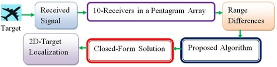
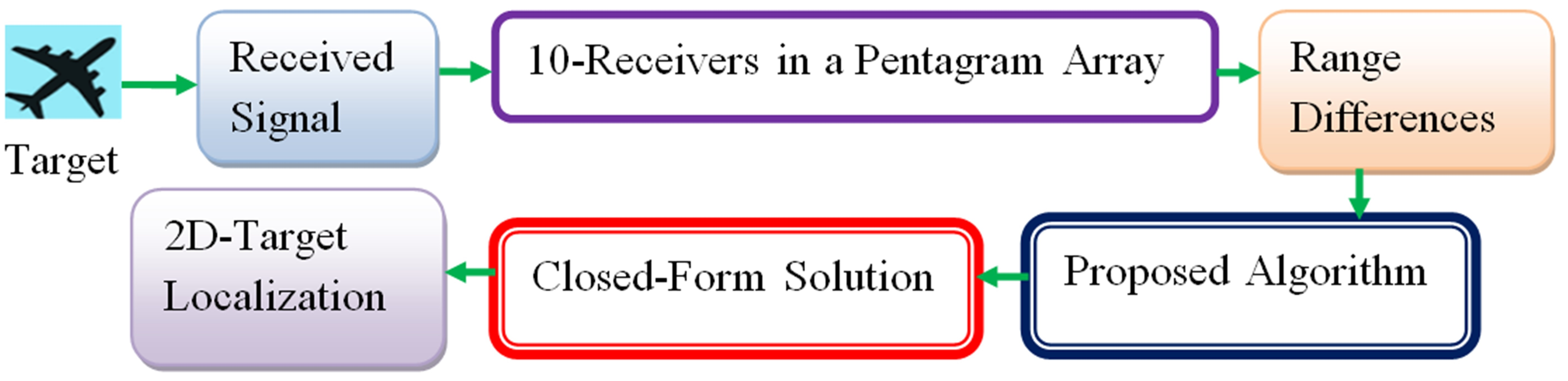
Reinvention and providing reliable and accurate target localization approaches are promising field studies. The main objective of this work is to present a new method for localization based on a closed-form solution to solve the aforementioned drawbacks of the SX and SI approaches.

According to this correspondence, this paper proposes a closed-form solution and its derivation of 2D target localization using a pentagram array.The choice of the pentagram array for developing this localization method was made based on the fixed number of receivers. The solution provided here is given using (N + 1 = 10 receivers, $\mathrm{N}=9$ RD measurements) a fixed number of receivers in the considered array. With this approach, target localization can be achieved directly from the positions of the array receivers and the RD measurements. As with our work in [26], where the same pentagram array paradigm was introduced, we considered the TDOAs, which are the time differences of the signal to transmit from the target to arrive at N + 1 = 10 receivers.

The receivers of the pentagram array lie in a subspace of dimension less than 3, which is not sufficient to determine the source location in three dimensions (3D). However, the performance of the method is provided only in two-dimensional target localization.

We considered a static problem using the RD measurements from a specific target location under a relatively far-spaced range for receivers and targets. Referring to the global positioning system (GPS) receiver’s calibration consideration in [27], we assumed an ionosphedriec time delay in the range of 20–100 ns due to the different receivers’ positions. Therefore, we assumed two values (20 and 50 ns) of time delay for the simulations. Hence, these time delays were converted to their corresponding two values of standard deviations ${\mathsf{\sigma }}_{\mathrm{d}\mathrm{i}}=6 \mathrm{m} \mathrm{a}\mathrm{n}\mathrm{d} 15 \mathrm{m}, \mathrm{f}\mathrm{o}\mathrm{r} \mathrm{i}= 1,\dots ,9$, respectively, by multiplying them by the speed of light (c). Then, two additive zero-mean Gaussian errors $N(0,{\sigma }^2)$ with these standard deviations were used to distort the RD measurements. It is well noted that all the adjusted values of coordinate sensor positions and target positions were selected under the passive radar scenario. The target localization in this work was calculated for four different target cases using the RD measurements for each target separately, applying the localization algorithm. Additionally, the theoretical accuracy results of the estimated target positions of this solution were illustrated, which relied on the introduced errors in RD measurements.

Target localization has a significant role in remote sensing applications. It provides information about the target, like spatial position, geographic location, distance, and speed, based on the acquired data. Applying the localization process accurately is crucial for identifying and monitoring purposes to understand static and dynamic targets or make planning decisions.

This paper is deemed to have a valuable contribution to the scope of signal processing, detection, and estimation, while the application of the proposed approach represents a significant process to solve the ambiguity in the association of the RD measurements in the case of observing multiple targets. So, its innovative points can be described as follows:

• Presenting a new approach for 2D target localization based on a closed-form solution.
• Derivation of the theoretical and mathematical formulation of the algorithm.
• Outlining the importance of combining the processes of the target’s direction of arrival (DOA) estimation and localization.
• Capability to be used in the initialization and application of the tracking techniques.
• Addressing the ghost target phenomenon by using the RD that corresponds to a certain target (reducing the spurious targets).
• Providing a single and accurate solution for localization outperforms the SX method.
• Removing the inconsistencies in the localization solutions presented by SX and SI.

The structure of this paper is as follows: In Section 2, we derived the problem of the target localization approach using a pentagram array. In Section 3, the derivation of the closed-form solution of the localization approach is given. The estimation accuracy of the proposed approach was included in Section 4. The numerical analysis and results of the performance of the localization method for the target position are presented in Section 5. Discussions were drawn in Section 6. In Section 7, conclusions and the future work of the study were included.

Notations: capital and small letters in boldface are used to indicate the matrixes and vectors, respectively, while lowercase letters stand for scalar quantities.

Superscripts: ${\left(·\right)}^T$ implies transpose; the symbol $\left(ā\right)$ denotes a unit vector; and the $‖·‖$ represents the norm of the matrix.

2. The Problem of the Localization Approach

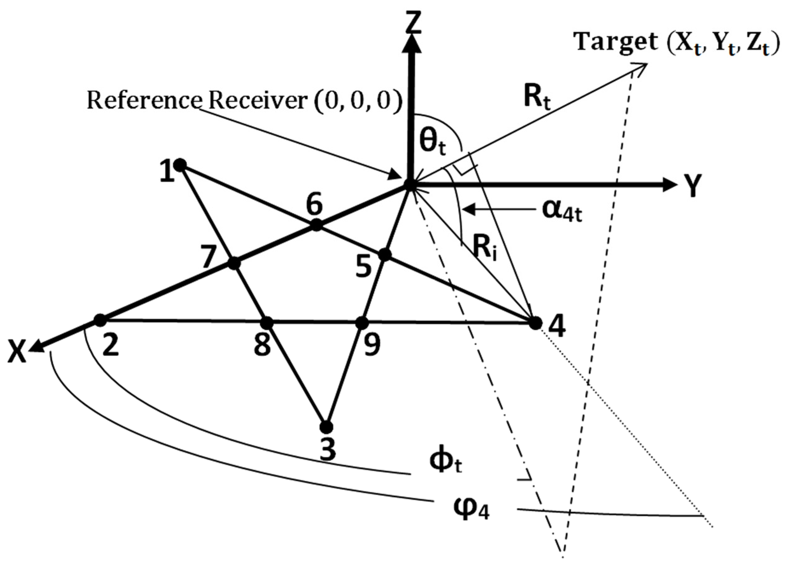
The localization system with pentagram array geometry is shown in Figure 1. In this system, we considered the case of one target and multiple (ten) receivers; this case can be used for multiple targets by dealing with every target in a separate manner. Additionally, to keep the generality, we assumed that the reference receiver is located at the position of the original point $\left(0, 0, 0\right)$ of the coordinate system. The number of receivers in the pentagram array is $\mathrm{N}+1=10$, including the reference one. The ith receiver is located at the position of the point with coordinates ${\mathbf{x}}_{\mathrm{i}}={\left[{\mathrm{x}}_{\mathrm{i}},{\mathrm{y}}_{\mathrm{i}},{\mathrm{z}}_{\mathrm{i}}\right]}^{\mathrm{T}}$ for $i=1:\mathrm{N}$. Here, only one fixed target was considered a point scatter, which is located at the position of coordinates ${\mathbf{x}}_{\mathrm{t}}={\left[{\mathrm{x}}_{\mathrm{t}},{\mathrm{y}}_{\mathrm{t}},{\mathrm{z}}_{\mathrm{t}}\right]}^{\mathrm{T}}$. According to this description, moving targets are not in the scope of this paper. ${\mathsf{\theta }}_t$ and ${\mathsf{\varphi }}_{\mathrm{t}}$ represent the direction of arrival (DOA) elevation and azimuth angles of the target, respectively.

The vector ${\overrightarrow{\mathrm{R}}}_{\mathrm{t}}$ of the length of the target range and the vector ${\overrightarrow{\mathrm{R}}}_{\mathrm{i}}$ of the length of the receiver’s ($\mathrm{i}$) range can be used to calculate the projection angle ${\mathsf{\alpha }}_{\mathrm{i}\mathrm{t}}$ between the two vectors as follows:

$$\cos {\mathsf{\alpha }}_{\mathrm{i}\mathrm{t}}=\frac{{\overrightarrow{\mathrm{R}}}_{\mathrm{t}}·{\overrightarrow{\mathrm{R}}}_{\mathrm{i}}}{‖{\overrightarrow{\mathrm{R}}}_{\mathrm{t}}‖‖{\overrightarrow{\mathrm{R}}}_{\mathrm{i}}‖}$$

(1)

where,

$${\overrightarrow{\mathrm{R}}}_{\mathrm{t}}=\left({\mathrm{x}}_{\mathrm{t}}-0\right){\mathrm{ā}}_{\mathrm{x}}+\left({\mathrm{y}}_{\mathrm{t}}-0\right){\mathrm{ā}}_{\mathrm{y}}+\left({\mathrm{z}}_{\mathrm{t}}-0\right){\mathrm{ā}}_{\mathrm{z}}={\mathrm{x}}_{\mathrm{t}}{\mathrm{ā}}_{\mathrm{x}}+{\mathrm{y}}_{\mathrm{t}}{\mathrm{ā}}_{\mathrm{y}}+{\mathrm{z}}_{\mathrm{t}}{\mathrm{ā}}_{\mathrm{z}}$$

(2)

$${\overrightarrow{\mathrm{R}}}_{\mathrm{i}}=\left({\mathrm{x}}_{\mathrm{i}}-0\right){\mathrm{ā}}_{\mathrm{x}}+\left({\mathrm{y}}_{\mathrm{i}}-0\right){\mathrm{ā}}_{\mathrm{y}}+\left({\mathrm{z}}_{\mathrm{i}}-0\right){\mathrm{ā}}_{\mathrm{z}}={\mathrm{x}}_{\mathrm{i}}{\mathrm{ā}}_{\mathrm{x}}+{\mathrm{y}}_{\mathrm{i}}{\mathrm{ā}}_{\mathrm{y}}+{\mathrm{z}}_{\mathrm{i}}{\mathrm{ā}}_{\mathrm{z} }(\mathrm{i}=1,\dots ,\mathrm{N})$$

(3)

$‖{\overrightarrow{\mathrm{R}}}_{\mathrm{t}}‖$ represents the Euclidian distance (${\mathrm{R}}_{\mathrm{t}}$) between the reference position and the position of the target (t), which is given by:

$${\mathrm{R}}_{\mathrm{t}}=‖{\overrightarrow{\mathrm{R}}}_{\mathrm{t}}‖=\sqrt{{{\mathrm{x}}_{\mathrm{t}}}^2+{{\mathrm{y}}_{\mathrm{t}}}^2+{{\mathrm{z}}_{\mathrm{t}}}^2}=‖{\mathrm{x}}_{\mathrm{t}}‖$$

(4)

and $‖{\overrightarrow{\mathrm{R}}}_{\mathrm{i}}‖$ is the Euclidian distance (${\mathrm{R}}_{\mathrm{i}}$) between the reference position and the position of the receiver ($\mathrm{i}$), which is given by:

$${\mathrm{R}}_{\mathrm{i}}=‖{\overrightarrow{\mathrm{R}}}_{\mathrm{i}}‖=\sqrt{{{\mathrm{x}}_{\mathrm{i}}}^2+{{\mathrm{y}}_{\mathrm{i}}}^2+{{\mathrm{z}}_{\mathrm{i}}}^2}\left(\mathrm{i}=1,\dots ,\mathrm{N}\right)$$

(5)

Substituting (2)–(5) into (1), we obtain:

$$\cos {\mathsf{\alpha }}_{\mathrm{i}\mathrm{t}}=\frac{\left({\mathrm{x}}_{\mathrm{i}}{\mathrm{ā}}_{\mathrm{x}}+{\mathrm{y}}_{\mathrm{i}}{\mathrm{ā}}_{\mathrm{y}}+{\mathrm{z}}_{\mathrm{i}}{\mathrm{ā}}_{\mathrm{z}}\right).\left({\mathrm{x}}_{\mathrm{t}}{\mathrm{ā}}_{\mathrm{x}}+{\mathrm{y}}_{\mathrm{t}}{\mathrm{ā}}_{\mathrm{y}}+{\mathrm{z}}_{\mathrm{t}}{\mathrm{ā}}_{\mathrm{z}}\right)}{\sqrt{{{\mathrm{x}}_{\mathrm{i}}}^2+{{\mathrm{y}}_{\mathrm{i}}}^2+{{\mathrm{z}}_{\mathrm{i}}}^2}\sqrt{{{\mathrm{x}}_{\mathrm{t}}}^2+{{\mathrm{y}}_{\mathrm{t}}}^2+{{\mathrm{z}}_{\mathrm{t}}}^2}} \mathrm{f}\mathrm{o}\mathrm{r} (\mathrm{i}=1,\dots ,\mathrm{N})$$

(6)

Applying the algebraic manipulation, we have:

$$\cos {\mathsf{\alpha }}_{\mathrm{i}\mathrm{t}}=\frac{\left({\mathrm{x}}_{\mathrm{i}}{\mathrm{x}}_{\mathrm{t}}+{\mathrm{y}}_{\mathrm{i}}{\mathrm{y}}_{\mathrm{t}}+{\mathrm{z}}_{\mathrm{i}}{\mathrm{z}}_{\mathrm{t}}\right)}{\sqrt{{{\mathrm{x}}_{\mathrm{i}}}^2+{{\mathrm{y}}_{\mathrm{i}}}^2+{{\mathrm{z}}_{\mathrm{i}}}^2}\sqrt{{{\mathrm{x}}_{\mathrm{t}}}^2+{{\mathrm{y}}_{\mathrm{t}}}^2+{{\mathrm{z}}_{\mathrm{t}}}^2}} \mathrm{f}\mathrm{o}\mathrm{r} (\mathrm{i}=1,\dots ,\mathrm{N})$$

(7)

Multiplying every side of Equation (7) by $\sqrt{{{\mathrm{x}}_{\mathrm{i}}}^2+{{\mathrm{y}}_{\mathrm{i}}}^2+{{\mathrm{z}}_{\mathrm{i}}}^2}$, we find:

$$\left(\sqrt{{{\mathrm{x}}_{\mathrm{i}}}^2+{{\mathrm{y}}_{\mathrm{i}}}^2+{{\mathrm{z}}_{\mathrm{i}}}^2}\right)\cos {\mathsf{\alpha }}_{\mathrm{i}\mathrm{t}}=\frac{\left({\mathrm{x}}_{\mathrm{i}}{\mathrm{x}}_{\mathrm{t}}+{\mathrm{y}}_{\mathrm{i}}{\mathrm{y}}_{\mathrm{t}}+{\mathrm{z}}_{\mathrm{i}}{\mathrm{z}}_{\mathrm{t}}\right)}{\sqrt{{{\mathrm{x}}_{\mathrm{t}}}^2+{{\mathrm{y}}_{\mathrm{t}}}^2+{{\mathrm{z}}_{\mathrm{t}}}^2}} \mathrm{f}\mathrm{o}\mathrm{r} (\mathrm{i}=1,\dots ,\mathrm{N})$$

(8)

According to our previous study in [26], the left part of Equation (8) represents the measured range differences (RDs) that correspond to the positions of the receivers of the pentagram array regarding the same target and the same reference position. So, we assume ${\mathrm{d}}_{\mathrm{i}}$ represents the RD of the sensor $\mathrm{i}$ relative to the reference receiver as follows:

$${\mathrm{d}}_{\mathrm{i}}=\left(\sqrt{{{\mathrm{x}}_{\mathrm{i}}}^2+{{\mathrm{y}}_{\mathrm{i}}}^2+{{\mathrm{z}}_{\mathrm{i}}}^2}\right)\cos {\mathsf{\alpha }}_{\mathrm{i}\mathrm{t}}={\mathrm{R}}_{\mathrm{i}}\cos {\mathsf{\alpha }}_{\mathrm{i}\mathrm{t}} \mathrm{f}\mathrm{o}\mathrm{r} (\mathrm{i}=1,\dots ,\mathrm{N})$$

(9)

where,

$$\cos {\alpha }_{it}=\sin {\mathsf{\theta }}_t\cos \left({\mathsf{\varphi }}_t-{\phi }_i\right)$$

(10)

and ${\mathsf{\phi }}_{\mathrm{i}}$ is the phase angle between the reference receiver and receiver $\mathrm{i}$. Then, substituting (9) into (8), we obtain:

$${\mathrm{d}}_{\mathrm{i}}=\frac{\left({\mathrm{x}}_{\mathrm{i}}{\mathrm{x}}_{\mathrm{t}}+{\mathrm{y}}_{\mathrm{i}}{\mathrm{y}}_{\mathrm{t}}+{\mathrm{z}}_{\mathrm{i}}{\mathrm{z}}_{\mathrm{t}}\right)}{\sqrt{{{\mathrm{x}}_{\mathrm{t}}}^2+{{\mathrm{y}}_{\mathrm{t}}}^2+{{\mathrm{z}}_{\mathrm{t}}}^2}}=\frac{\left({\mathrm{x}}_{\mathrm{i}}{\mathrm{x}}_{\mathrm{t}}+{\mathrm{y}}_{\mathrm{i}}{\mathrm{y}}_{\mathrm{t}}+{\mathrm{z}}_{\mathrm{i}}{\mathrm{z}}_{\mathrm{t}}\right)}{{\mathrm{R}}_{\mathrm{t}}} \mathrm{f}\mathrm{o}\mathrm{r} (\mathrm{i}=1,\dots ,\mathrm{N})$$

(11)

Then,

$${\mathrm{d}}_{\mathrm{i}}{\mathrm{R}}_{\mathrm{t}}=\left({\mathrm{x}}_{\mathrm{i}}{\mathrm{x}}_{\mathrm{t}}+{\mathrm{y}}_{\mathrm{i}}{\mathrm{y}}_{\mathrm{t}}+{\mathrm{z}}_{\mathrm{i}}{\mathrm{z}}_{\mathrm{t}}\right) \mathrm{f}\mathrm{o}\mathrm{r} (\mathrm{i}=1,\dots ,\mathrm{N})$$

(12)

So, we can write the spatial coordinate vectors of the $\mathrm{N}$ sensors as follows:

$${\mathbf{x}}_{\mathrm{i}}\triangleq \left[\begin{array}{c}{\mathrm{x}}_{\mathrm{i}}\\ {\mathrm{y}}_{\mathrm{i}}\\ {\mathrm{z}}_{\mathrm{i}}\end{array}\right], \mathrm{f}\mathrm{o}\mathrm{r} (\mathrm{i}=1,\dots ,\mathrm{N})$$

(13)

where ${\mathbf{x}}_{\mathrm{i}}$ is the ${\mathrm{i}}_{\mathrm{t}\mathrm{h}}$ receiver position. The unknown target position ${\mathbf{x}}_{\mathrm{t}}$ is defined by:

$${\mathbf{x}}_{\mathrm{t}}\triangleq \left[\begin{array}{c}{\mathrm{x}}_{\mathrm{t}}\\ {\mathrm{y}}_{\mathrm{t}}\\ {\mathrm{z}}_{\mathrm{t}}\end{array}\right]$$

(14)

Now, we can define a general matrix for $\mathrm{N}$ receivers as follows:

$$\mathbf{S}\triangleq {\left[\begin{array}{ccc}{\mathrm{x}}_1& {\mathrm{y}}_1& {\mathrm{z}}_1\\ {\mathrm{x}}_2& {\mathrm{y}}_2& {\mathrm{z}}_2\\ ⋮& ⋮& ⋮\\ {\mathrm{x}}_{\mathrm{N}}& {\mathrm{y}}_{\mathrm{N}}& {\mathrm{z}}_{\mathrm{N}}\end{array}\right]}_{\mathrm{N}\times 3}$$

(15)

Then, we also describe the vector of the range distances (RDs) for $\mathrm{N}$ receivers as below:

$$\mathbf{d}\triangleq {\left[\begin{array}{c}{\mathrm{d}}_1\\ {\mathrm{d}}_2\\ ⋮\\ {\mathrm{d}}_{\mathrm{N}}\end{array}\right]}_{\mathrm{N}\times 1}$$

(16)

Now, it is clear that the general matrix $\mathrm{S}$ in (15) contains only the pure given data of the receivers, and the vector $\mathrm{d}$ in (16) exclusively includes the data with their noise-corrupted measurements. Using the notations in (15) and (16), we can write (12) in matrix notation form for $\mathrm{N}$ receivers as below:

$$\mathbf{S}{\mathbf{x}}_t=\mathbf{d}{\mathrm{R}}_{\mathrm{t}}$$

(17)

Equation (17) describes a linear system and contains four unknown variables: ${\mathrm{x}}_{\mathrm{t}},{\mathrm{y}}_{\mathrm{t}},\mathrm{a}\mathrm{n}\mathrm{d} {\mathrm{z}}_{\mathrm{t}}$ for the target position, and ${\mathrm{R}}_{\mathrm{t}}$ for the target-reference receiver range. The estimated solution of the target position in the least squares sense when ${\mathrm{R}}_{\mathrm{t}}$ is known can be obtained as follows:

$${\widehat{\mathbf{x}}}_t={\left({\mathbf{S}}^{\mathrm{T}}\mathbf{S}\right)}^{-1}{\mathbf{S}}^{\mathrm{T}}\mathbf{d}{\mathrm{R}}_{\mathrm{t}}$$

(18)

In order to solve for the target position (${\widehat{\mathbf{x}}}_t$) using (18), the value of the variable ${\mathrm{R}}_{\mathrm{t}}$ must be available. In the literature on TDOA localization, there are two ways that were used to obtain an estimated target-to-reference receiver distance ${\mathrm{R}}_{\mathrm{t}}$: one is known as the spherical-interpolation (SI) technique [1,24], where an estimated ${\mathrm{R}}_{\mathrm{t}}$ is calculated from a quotient of the mathematical division process. The other one is the spherical-intersection (SX) technique [8,9], in which an estimated ${\mathrm{R}}_{\mathrm{t}}$ is achieved using a quadratic equation. The authors in [25] explained that the SX technique is much more robust to measurement errors in the case of a TDOA system compared to the SI technique. Finally, after obtaining the value of ${\mathrm{R}}_{\mathrm{t}}$, substitute this value into (18) to find the estimated target (position) location (${\widehat{\mathbf{x}}}_t$).

Now, consider a special case of ${\mathrm{R}}_{\mathrm{t}}$ by defining a new vector as follows:

$$\mathbf{a}\triangleq {\left({\mathbf{S}}^{\mathrm{T}}\mathbf{S}\right)}^{-1}{\mathbf{S}}^{\mathrm{T}}\mathbf{d}=\left[\begin{array}{c}{\mathrm{a}}_1\\ {\mathrm{a}}_2\\ {\mathrm{a}}_3\end{array}\right]$$

(19)

So, (18) becomes the following:

$${\widehat{\mathbf{x}}}_{\mathrm{t}}=\mathrm{a}{\mathrm{R}}_{\mathrm{t}}$$

(20)

Using the definitions in (19) and (20), we can write the following relationship:

$${\mathbf{x}}_{\mathrm{t}}=\left[\begin{array}{c}{\mathrm{x}}_{\mathrm{t}}\\ {\mathrm{y}}_{\mathrm{t}}\\ {\mathrm{z}}_{\mathrm{t}}\end{array}\right]=\left[\begin{array}{c}{\mathrm{a}}_1{\mathrm{R}}_{\mathrm{t}}\\ {\mathrm{a}}_2{\mathrm{R}}_{\mathrm{t}}\\ {\mathrm{a}}_3{\mathrm{R}}_{\mathrm{t}}\end{array}\right]$$

(21)

Substituting (21) in (4) and applying some algebraic manipulations, we find the following:

$${\mathrm{R}}_{\mathrm{t}}=\sqrt{{{(\mathrm{a}}_1{\mathrm{R}}_{\mathrm{t}})}^2+{{(\mathrm{a}}_2{\mathrm{R}}_{\mathrm{t}})}^2+{{(\mathrm{a}}_3{\mathrm{R}}_{\mathrm{t}})}^2}$$

(22)

then,

$${\left({\mathrm{R}}_{\mathrm{t}}\right)}^2={{(\mathrm{a}}_1{\mathrm{R}}_{\mathrm{t}})}^2+{{(\mathrm{a}}_2{\mathrm{R}}_{\mathrm{t}})}^2+{{(\mathrm{a}}_3{\mathrm{R}}_{\mathrm{t}})}^2$$

(23)

or

$${\left({\mathrm{R}}_{\mathrm{t}}\right)}^2(1-({{\mathrm{a}}_1}^2+{{\mathrm{a}}_2}^2+{{\mathrm{a}}_3}^2\left)\right)=0$$

(24)

so,

$$({{\mathrm{a}}_1}^2+{{\mathrm{a}}_2}^2+{{\mathrm{a}}_3}^2)=1$$

(25)

Equation (25) states that the sum of the squares of ${\mathrm{a}}_1$, ${\mathrm{a}}_2$, and ${\mathrm{a}}_3$ is equal to unity, which represents the equation for a unit sphere.

It is clear that the solutions of (25) are all the points on the surface of the sphere with a radius of unity, which means ${\mathrm{R}}_{\mathrm{t}}=1$. Thus, substituting this value for ${\mathrm{R}}_{\mathrm{t}}$ in (21) yields the values of ${\mathrm{a}}_1$, ${\mathrm{a}}_2$, and ${\mathrm{a}}_3$,which represent the coordinate points of the target (location) position as below:

$${\mathrm{a}}_1={\mathrm{x}}_{\mathrm{t}}=\cos {\mathsf{\varphi }}_{\mathrm{t}}\sin {\mathsf{\theta }}_{\mathrm{t}}$$

(26)

$${\mathrm{a}}_2={\mathrm{y}}_{\mathrm{t}}=\sin {\mathsf{\varphi }}_{\mathrm{t}}\sin {\mathsf{\theta }}_{\mathrm{t}}$$

(27)

$${\mathrm{a}}_3={\mathrm{z}}_{\mathrm{t}}=\cos {\mathsf{\theta }}_{\mathrm{t}}$$

(28)

where ${\mathsf{\varphi }}_{\mathrm{t}}$ is the DOA azimuth angle of the target, ranging from 0 to 2π, and ${\mathsf{\theta }}_{\mathrm{t}}$ is the DOA elevation angle of the target, ranging from 0 to π, as shown in Figure 1. For investigating the performance of the method, we can substitute the same value of ${\mathrm{R}}_{\mathrm{t}}=1$ in (18), which must obtain the same results for ${\mathrm{x}}_{\mathrm{t}}$, ${\mathrm{y}}_{\mathrm{t}}$, and ${\mathrm{z}}_{\mathrm{t}}$ as the target (location) position.

3. Closed-Form Solution of the Localization Approach

We show that the closed-form equation in (18) for target localization depends on ${\mathrm{R}}_{\mathrm{t}}$. The difficulty of (18) lies in calculating the value of ${\mathrm{R}}_{\mathrm{t}}$ using the two aforementioned spherical methods. In SX [8,9], where ${\mathrm{R}}_{\mathrm{t}}$ is calculated using a quadratic equation in which more (two real or complex-valued) solutions for ${\mathrm{R}}_{\mathrm{t}}$ exist, discerning which solution corresponds to the correct target requires considering additional aspects or physical logics, such as the number of transmitters and receivers and their symmetrical distribution geometry. As an example, the authors in [4] used the positive height method of estimation for selecting the correct solution when dealing with flying targets, although it is not a perfect method in radar applications in some cases. For the SI [1,24] method, the authors in [4] show that the estimated value ${\widehat{\mathrm{R}}}_t$ of ${\mathrm{R}}_{\mathrm{t}}$ obtained by this method everywhere differs from the value of $‖{\widehat{\mathbf{x}}}_t‖,$ which is the result of substituting ${\widehat{\mathrm{R}}}_t$ in (18), and also differs from that of the SX method. This means that ${\widehat{\mathrm{R}}}_t,$ calculated by the SI method, has not been well-approved by the condition ${\widehat{\mathrm{R}}}_{\mathrm{t}}=‖{\widehat{\mathbf{x}}}_{\mathrm{t}}‖$. However, these differences in the estimated results of ${\mathrm{R}}_{\mathrm{t}}$ result in a notable error in target position estimation. Moreover, based on the estimated value of ${\mathrm{R}}_{\mathrm{t}},$ a contradiction appears between the two methods. According to the results presented in [25], SI outperforms SX in the TDOA-considered case, while SX performs better than SI in the passive radar scenario, as shown by the results in [4].

Now, our aim is to find a simple target (position) localization formula for (${\widehat{\mathbf{x}}}_t$) in (18) by eliminating ${\mathrm{R}}_{\mathrm{t}}$. This can be obtained by considering the basic relationship that is satisfied by the RDs, as follows:

$${\mathrm{d}}_{\mathrm{i}}={\mathrm{R}}_{\mathrm{i}\mathrm{t}}-{\mathrm{R}}_{\mathrm{t}} \mathrm{f}\mathrm{o}\mathrm{r} (\mathrm{i}=1,\dots ,\mathrm{N})$$

(29)

where ${\mathrm{R}}_{\mathrm{i}\mathrm{t}}$ is the Euclidian distance between the target and receiver $\mathrm{i}$, which is given by:

$${\mathrm{R}}_{\mathrm{i}\mathrm{t}}=\sqrt{{{(\mathrm{x}}_{\mathrm{i}}-{\mathrm{x}}_{\mathrm{t}})}^2+{{(\mathrm{y}}_{\mathrm{i}}-{\mathrm{y}}_{\mathrm{t}})}^2+{({\mathrm{z}}_{\mathrm{i}}-{\mathrm{z}}_{\mathrm{t}})}^2} \mathrm{f}\mathrm{o}\mathrm{r} (\mathrm{i}=1,\dots ,\mathrm{N})$$

(30)

Then, (29) can be rewritten using (4) and (30) as follows:

$${\mathrm{d}}_{\mathrm{i}}=\sqrt{{{(\mathrm{x}}_{\mathrm{i}}-{\mathrm{x}}_{\mathrm{t}})}^2+{{(\mathrm{y}}_{\mathrm{i}}-{\mathrm{y}}_{\mathrm{t}})}^2+{({\mathrm{z}}_{\mathrm{i}}-{\mathrm{z}}_{\mathrm{t}})}^2}-\sqrt{{{\mathrm{x}}_{\mathrm{t}}}^2+{{\mathrm{y}}_{\mathrm{t}}}^2+{{\mathrm{z}}_{\mathrm{t}}}^2} \mathrm{f}\mathrm{o}\mathrm{r} (\mathrm{i}=1,\dots ,\mathrm{N})$$

(31)

We perform some mathematical manipulation on (31) to yield the following:

$${\mathrm{x}}_{\mathrm{i}}{\mathrm{x}}_{\mathrm{t}}+{\mathrm{y}}_{\mathrm{i}}{\mathrm{y}}_{\mathrm{t}}+{\mathrm{z}}_{\mathrm{i}}{\mathrm{z}}_{\mathrm{t}}+{\mathrm{d}}_{\mathrm{i}}{\mathrm{R}}_{\mathrm{t}}=\frac{1}{2}({{\mathrm{x}}_{\mathrm{i}}}^2+{{\mathrm{y}}_{\mathrm{i}}}^2+{{\mathrm{z}}_{\mathrm{i}}}^2-{{\mathrm{d}}_{\mathrm{i}}}^2) \mathrm{f}\mathrm{o}\mathrm{r} (\mathrm{i}=1,\dots ,\mathrm{N})$$

(32)

From (12), by substituting the value of the first part of the left-hand side of (32) and simplifying the result, we find the following:

$${\mathrm{R}}_{\mathrm{t}}=\frac{1}{4{\mathrm{d}}_{\mathrm{i}}}({{\mathrm{x}}_{\mathrm{i}}}^2+{{\mathrm{y}}_{\mathrm{i}}}^2+{{\mathrm{z}}_{\mathrm{i}}}^2-{{\mathrm{d}}_{\mathrm{i}}}^2) \mathrm{f}\mathrm{o}\mathrm{r} (\mathrm{i}=1,\dots ,\mathrm{N})$$

(33)

So, we can define a new vector as follows:

$$\mathbf{z}=\frac{1}{4}{\left[\begin{array}{c}{{\mathrm{x}}_1}^2+{{\mathrm{y}}_1}^2+{{\mathrm{z}}_1}^2-{{\mathrm{d}}_1}^2\\ {{\mathrm{x}}_2}^2+{{\mathrm{y}}_2}^2+{{\mathrm{z}}_2}^2-{{\mathrm{d}}_2}^2\\ ⋮\\ {{\mathrm{x}}_{\mathrm{N}}}^2+{{\mathrm{y}}_{\mathrm{N}}}^2+{{\mathrm{z}}_{\mathrm{N}}}^2-{{\mathrm{d}}_{\mathrm{N}}}^2\end{array}\right]}_{\mathrm{N}\times 1}$$

(34)

Then, using matrix notations of (16) and (34), (33) can be written as follows:

$${\mathrm{R}}_{\mathrm{t}}=\frac{\mathit{z}}{\mathbf{d}}={\left({\mathbf{d}}^{\mathrm{T}}\mathbf{d}\right)}^{-1}{\mathbf{d}}^{\mathrm{T}}\mathbf{z}$$

(35)

The value of ${\mathrm{R}}_{\mathrm{t}}$ in Equation (35) significantly depends on the accuracy of the TDOA measurements. As the delays are typically not measured precisely, we consider ${\mathrm{R}}_{\mathrm{t}}$ to be an estimated solution, i.e.${,\mathrm{R}}_{\mathrm{t}}={\widehat{\mathrm{R}}}_{\mathrm{t}}.$ Now, inserting (35) into (18) yields the following:

$${\widehat{\mathbf{x}}}_{\mathrm{t}}={\left({\mathbf{S}}^{\mathrm{T}}\mathbf{S}\right)}^{-1}{\mathbf{S}}^{\mathrm{T}}\mathbf{d}{(\left({\mathbf{d}}^{\mathrm{T}}\mathbf{d}\right)}^{-1}{\mathbf{d}}^{\mathrm{T}}\mathbf{z})$$

(36)

Finally, the formula for target localization in (36) has only three variables (${\mathrm{x}}_{\mathrm{t}},{\mathrm{y}}_{\mathrm{t}},\mathrm{a}\mathrm{n}\mathrm{d} {\mathrm{z}}_{\mathrm{t}}$) that describe a linear system whose closed-form solution can be used to estimate the target position ${\widehat{\mathbf{x}}}_{\mathrm{t}}$ using only the data of the receivers locations and their corresponding RDs.

4. Accuracy of the Estimated Target Position

The accuracy of the method depends on the accuracy of the RDs parameters. In such applications, the signal-to-noise ratio and the range resolution criterion are used to estimate the accuracy of the measurements [4]. The estimated solution of the target position that was obtained by (36) was calculated using the variances of the RDs, which realize Equation (29). Using these variances, which represent the accuracy of the RDs, we can calculate the accuracy of the method in the Cartesian coordinates.

Let ${\sigma }_{Di}^2$ be the variance of the RD corresponding to the ith receiver. Then we can give an expression to the covariance matrix $\mathbf{R}$ (a diagonal matrix that contains the $\mathrm{N}$-vector of variances for $\mathrm{N}$ receivers) of the RDs by the following:

$${\mathbf{R}}_{\mathrm{N}\times \mathrm{N}}=\mathrm{E}\left[{\mathbf{d}\mathbf{d}}^{\mathrm{T}}\right]=\mathrm{d}\mathrm{i}\mathrm{a}\mathrm{g}\left(\left[{\mathsf{\sigma }}_{\mathrm{D}1}^2,{\mathsf{\sigma }}_{\mathrm{D}2}^2,\dots .,{\mathsf{\sigma }}_{\mathrm{D}\mathrm{N}}^2\right]\right)$$

(37)

The covariance matrix is difficult to find in an easy way due to the nonlinear relationship between the RDs and the estimated target position. In [24], a formulation was presented that can be used to give an approximate expression for the covariance matrix. The covariance matrix of the estimated position can be approximated using a first-order Taylor series expansion as follows:

$${\mathbf{W}}_{2\times 2}=\mathrm{E}\left[{{\widehat{\mathbf{x}}}_{\mathrm{t}}{\widehat{\mathbf{x}}}_{\mathrm{t}}}^{\mathrm{T}}\right]\approx \left(\frac{\partial {\mathbf{x}}_{\mathrm{t}}}{\partial \mathbf{d}}\right)\mathbf{R}{\left(\frac{\partial {\mathbf{x}}_{\mathrm{t}}}{\partial \mathbf{d}}\right)}^{\mathrm{T}}$$

(38)

where ${\left(\frac{\partial {\mathbf{x}}_{\mathrm{t}}}{\partial \mathbf{d}}\right)}_{2\times N}$ represents the Jacobian, which can be achieved by making a differentiation of Equation (17) with respect to d:

$$\mathbf{S}\frac{\partial {\mathbf{x}}_{\mathrm{t}}}{\partial \mathbf{d}}=\frac{\partial \left({\mathbf{d}\mathrm{R}}_{\mathrm{t}}\right)}{\partial \mathbf{d}}$$

(39)

Then, the derivation of the right-hand side of the above equation is given the following:

$$\frac{\partial \left({\mathbf{d}\mathrm{R}}_{\mathrm{t}}\right)}{\partial \mathbf{d}}=\mathbf{I}{\mathrm{R}}_{\mathrm{t}}+\mathbf{d}\frac{\partial {\mathrm{R}}_{\mathrm{t}}}{\partial \mathbf{d}}$$

(40)

where I is the identity matrix. Then, using the chain rule, we can calculate $\frac{\partial {\mathrm{R}}_{\mathrm{t}}}{\partial \mathbf{d}}$, such as follows:

$$\frac{\partial {\mathrm{R}}_{\mathrm{t}}}{\partial \mathbf{d}}=\frac{\partial {\mathrm{R}}_{\mathrm{t}}}{\partial {\mathbf{x}}_{\mathrm{t}}}\frac{\partial {\mathbf{x}}_{\mathrm{t}}}{\partial \mathbf{d}}=\frac{{{\mathbf{x}}_{\mathrm{t}}}^{\mathrm{T}}}{‖{\mathbf{x}}_{\mathrm{t}}‖}\frac{\partial {\mathbf{x}}_{\mathrm{t}}}{\partial \mathbf{d}}$$

(41)

Substituting (40) and (41) in (39), we find the following:

$$\mathbf{S}\frac{\partial {\mathbf{x}}_{\mathrm{t}}}{\partial \mathbf{d}}=\mathbf{I}{\mathrm{R}}_{\mathrm{t}}+\mathbf{d}\frac{{{\mathbf{x}}_{\mathrm{t}}}^{\mathrm{T}}}{‖{\mathbf{x}}_{\mathrm{t}}‖}\frac{\partial {\mathbf{x}}_{\mathrm{t}}}{\partial \mathbf{d}}$$

(42)

Then, we can obtain the Jacobian matrix after rearranging Equation (42) as below:

$$\frac{\partial {\mathbf{x}}_{\mathrm{t}}}{\partial \mathbf{d}}\left(\mathbf{S}-\mathbf{d}\frac{{{\mathbf{x}}_{\mathrm{t}}}^{\mathrm{T}}}{‖{\mathbf{x}}_{\mathrm{t}}‖}\right)=\mathbf{I}{\mathrm{R}}_{\mathrm{t}}$$

(43)

Now, define a new matrix B as follows:

$$\mathbf{B}=\mathbf{S}-\mathbf{d}\frac{{{\mathbf{x}}_{\mathrm{t}}}^{\mathrm{T}}}{‖{\mathbf{x}}_{\mathrm{t}}‖}$$

(44)

So, Equation (43) can be expressed as follows:

$$\frac{\partial {\mathbf{x}}_{\mathrm{t}}}{\partial \mathbf{d}}={\left({\mathbf{B}}^{\mathrm{T}}\mathbf{B}\right)}^{-1}{\mathbf{B}}^{\mathrm{T}}\left(\mathbf{I}{\mathrm{R}}_{\mathrm{t}}\right)$$

(45)

Finally, substitute (45) in (38) to find the covariance matrix ${\mathbf{W}}_{2\times 2}$ of the estimated target position, whose diagonal values indicate the variances of the estimated target position error in the x and y coordinates.

5. Numerical Results

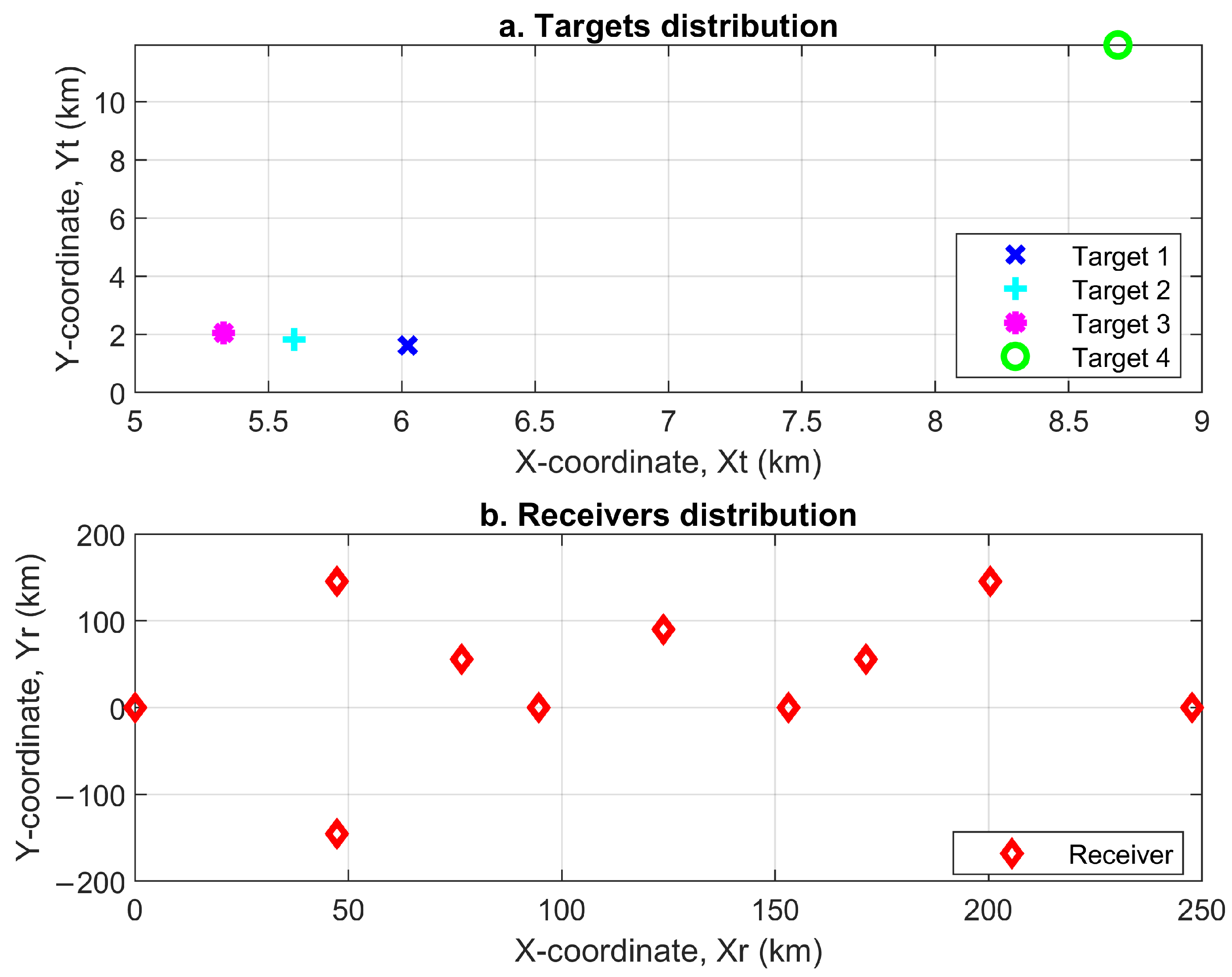
This paper is an extension of our previous work presented in [26]. The pentagram array with ten receivers (the fixed number of receivers in the array) of the mentioned study was used to investigate the performance of this algorithm. We carried out numerical analysis simulations with MATLAB/R2018a computer software using the RD measurements. The parameters of the four different targets are listed in

Table 1. The parameters of the four different targets.

Target No.	x-Offset (km)	y-Offset (km)	Rt (km)
1	6.02255	1.61374	6.235
2	5.59697	1.81857	5.885
3	5.33261	2.04700	5.712
4	8.68453	11.95323	14.775

.

The assumption of the targets and their distribution in only two dimensions was selected according to the restriction of this pentagram array paradigm. We assumed a relatively far target (target No. 1), two relatively close targets (both targets No. 2 and No. 3), and a faraway target (target No. 4). Additionally, all four targets were considered independent of each other. The simulation result of the distribution of the targets in the two dimensions is shown in Figure 2a, according to the parameters listed in Table 1. The blue mark (x), cyan mark (+), magenta mark (*), and green mark (o) indicate target 1, target 2, target 3, and target 4, respectively.

The positions of the receivers (N + 1 = 10) in the pentagram array for the position estimation of these four targets are listed in

Table 2. The positions of the receivers of the pentagram array.

Receiver No.	x-Offset (km)	y-Offset (km)	z-Offset (km)
Reference	0.0000	0.0000	0.0000
1	47.30303	−145.58377	0.00000
2	247.69553	0.00000	0.00000
3	200.38989	145.59178	0.00000
4	47.30303	145.58378	0.00000
5	76.54312	55.61183	0.00000
6	94.61250	0.00000	0.00000
7	153.08303	0.00000	0.00000
8	171.21456	55.63098	0.00000
9	123.84677	89.97994	0.00000

. The receivers were placed in a 2D subspace, which is less than three and not sufficient for 3D localization. This leads to making the z-offset of all positions of the receivers zero in Table 2. These receiver positions were set and distributed over a relatively wide area. The array layout for the receiver’s distribution using the data listed in Table 2 is shown in Figure 2b. The red marks (diamond) represent the ten positions of the array receivers in both x and y coordinates.

Then, two additive zero-mean Gaussian errors $N(0,{\sigma }^2)$ with standard deviations o ${\mathsf{\sigma }}_{\mathrm{d}\mathrm{i}}=6 \mathrm{m} \mathrm{a}\mathrm{n}\mathrm{d} 15 \mathrm{m}, \mathrm{f}\mathrm{o}\mathrm{r} i=1,\dots ,9 \mathrm{a}\mathrm{r}\mathrm{e}$ used to distort the RD measurements of the four targets in the simulations.

The main purpose of this part is to test the validity of the new approach of (36) for target localization, which was derived based on the formula of (18) and represents its closed-form solution. This means its validity significantly relies on the validity of (18). Therefore, we will investigate the performance of (18) for 2D localization of the four targets. The realization of (18) requires the value of ${\mathrm{R}}_{\mathrm{t}}$ to be known. The value of ${\mathrm{R}}_{\mathrm{t}}$ was obtained by (35). First, we conducted the simulations under distortion of the RD by an additive zero-mean Gaussian error with ${\mathsf{\sigma }}_{\mathrm{d}\mathrm{i}}=6 \mathrm{m}, \mathrm{f}\mathrm{o}\mathrm{r} i=1,\dots ,9$. 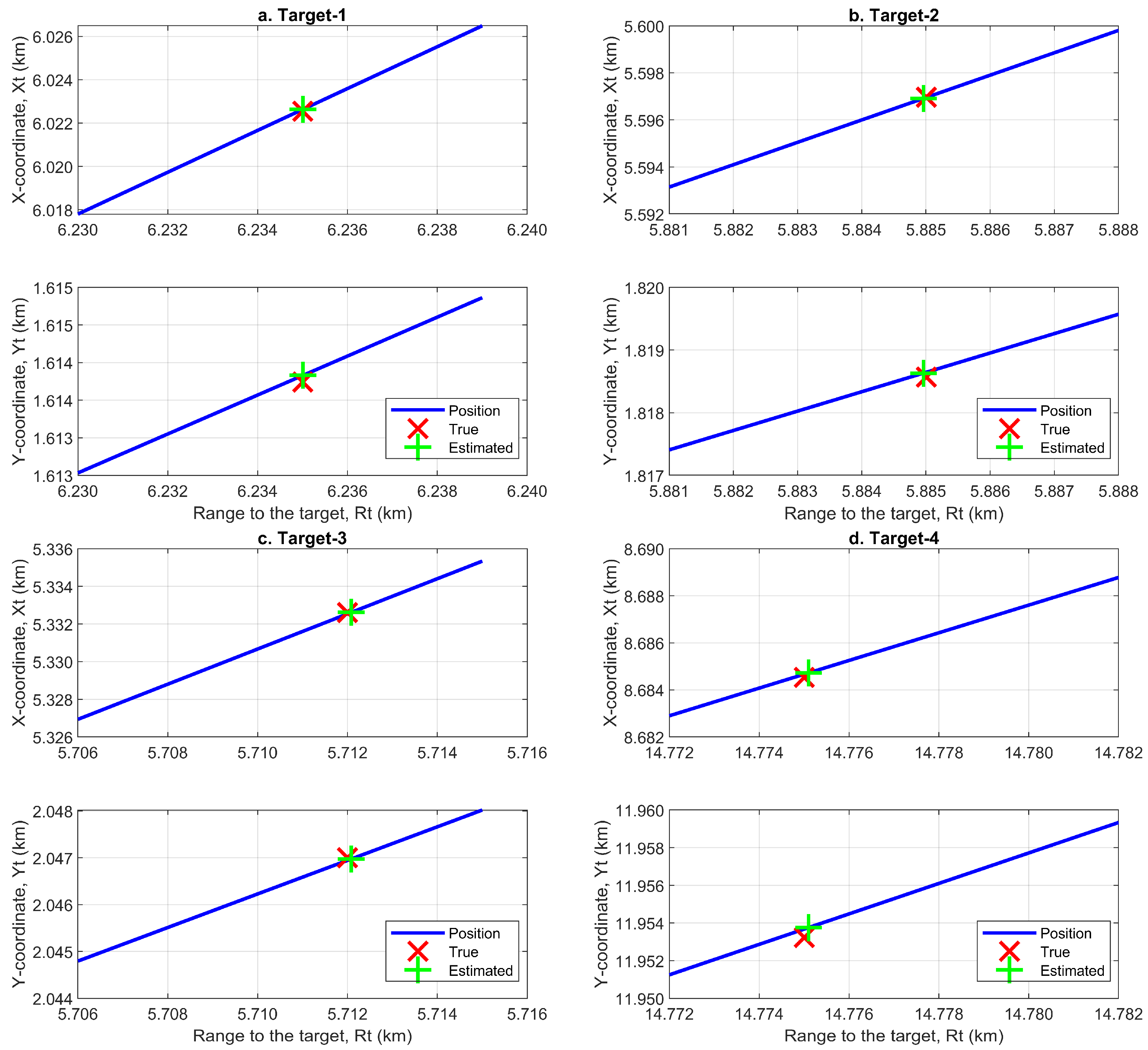The estimated coordinates ${\widehat{\mathrm{x}}}_{\mathrm{t}} \mathrm{a}\mathrm{n}\mathrm{d} {\widehat{\mathrm{y}}}_{\mathrm{t}}$ of the estimated 2D target (location) position $\left({\widehat{\mathbf{x}}}_{\mathrm{t}}\right)$ calculated according to (18) for four targets, in this case using the values of ${\mathrm{R}}_{\mathrm{t}}$ according to (35), are shown in Figure 3a–d, respectively, for only one round of simulation.

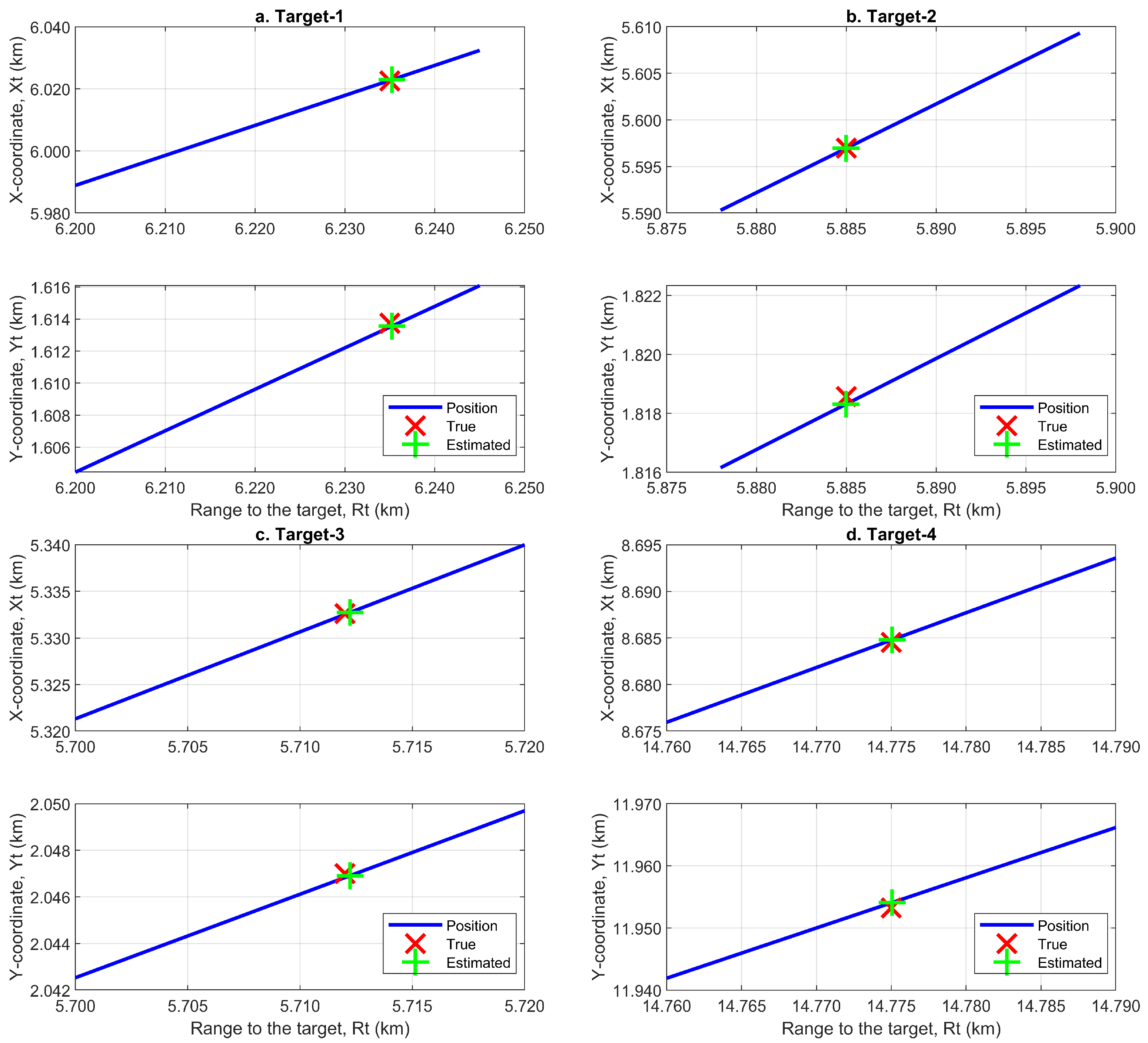
Second, we regenerated the simulations under distortion of the RD by another additive zero-mean Gaussian error with ${\mathsf{\sigma }}_{\mathrm{d}\mathrm{i}}=15 \mathrm{m}, \mathrm{f}\mathrm{o}\mathrm{r} i=1,\dots ,9$. Here, the results of the estimated coordinates ${\widehat{\mathrm{x}}}_{\mathrm{t}} \mathrm{a}\mathrm{n}\mathrm{d} {\widehat{\mathrm{y}}}_{\mathrm{t}}$ of the estimated 2D target (location) position $\left({\widehat{\mathbf{x}}}_t\right)$ by (18) for the same four targets are shown in Figure 4a–d.

It is clear from Figure 3a–d and Figure 4a–d and according to (18) that the position varies linearly (represented by the blue lines) with ${\mathrm{R}}_{\mathrm{t}}$. The red mark (x) indicates the true positions in the x and y coordinates of the four targets (values in Table 1), which, due to the RD errors, are not located on the blue line, while the green mark (+) indicates the estimated positions in the x and y coordinates of the four targets using the algorithm of the formula in (18). All the estimated positions fully correspond with the true positions in the x and y coordinates, even for different and large errors. This accuracy in the estimated positions $\left({\widehat{\mathbf{x}}}_t\right)$ and ${\widehat{\mathrm{R}}}_{\mathrm{t}}$ indicates the validity of this method for target localization.

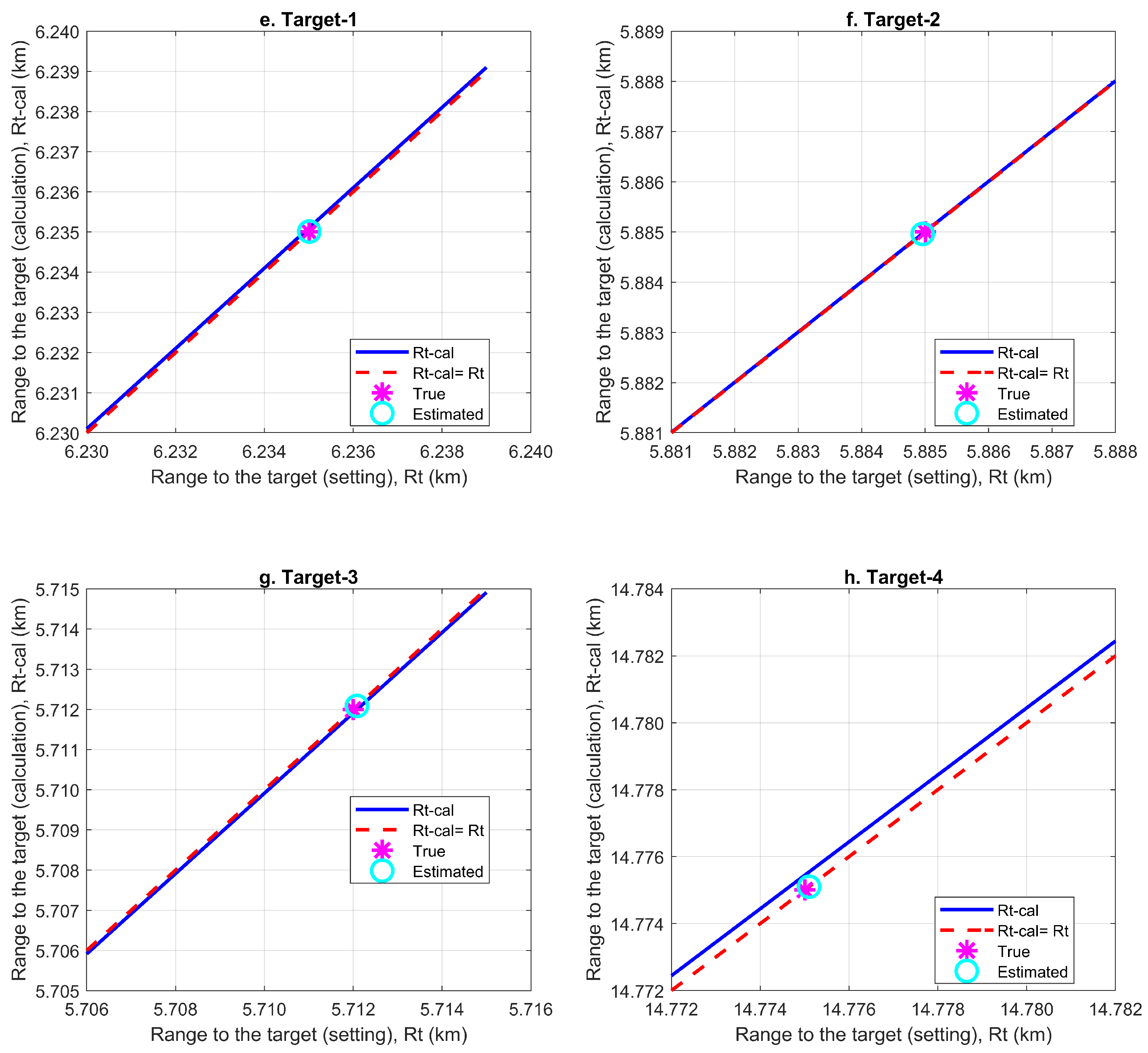
The estimated values of ${\mathrm{R}}_{\mathrm{t}}$ by (35) were used in (18) to obtain the estimated positions $\left({\widehat{\mathrm{x}}}_{\mathrm{t}}\right)$. To examine the enforcement of the term ${\mathrm{R}}_{\mathrm{t}}=‖{\widehat{\mathrm{x}}}_{\mathrm{t}}‖$ during the derivation of the algorithm, Figure 5e–h shows the simulation results of the estimated range to the target (Rt using (18)) versus the range to the target obtained by ${\mathrm{R}}_{\mathrm{t}}=‖{\widehat{\mathrm{x}}}_{\mathrm{t}}‖$ with standard deviation ${\mathsf{\sigma }}_{\mathrm{d}\mathrm{i}}=6 \mathrm{m}$.

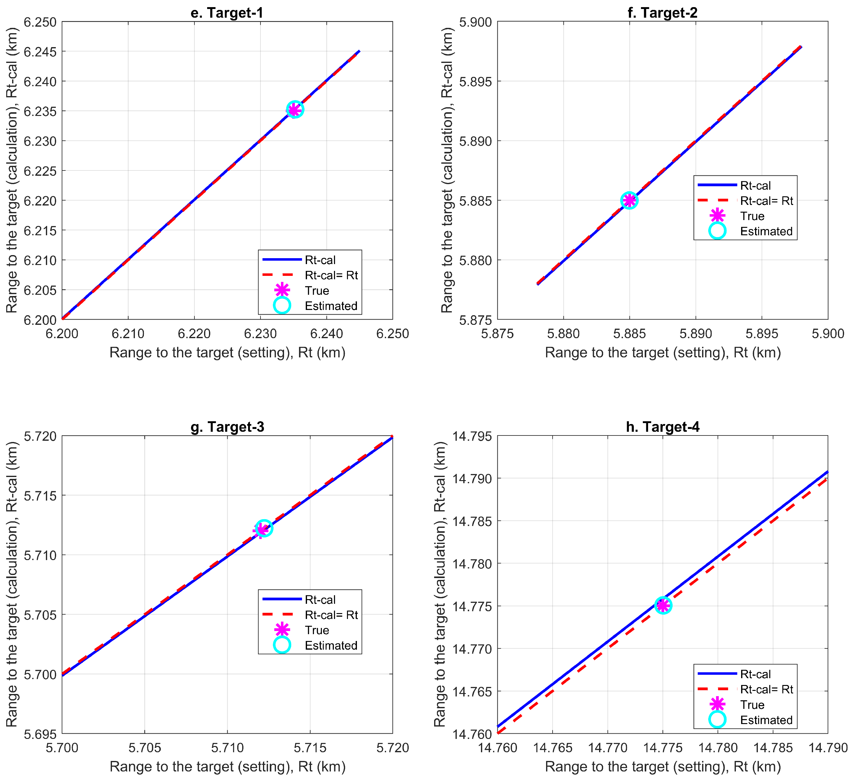
The simulation results of the estimated range to the target (Rt using (18)) versus the range to the target obtained by ${\mathrm{R}}_{\mathrm{t}}=‖{\widehat{\mathrm{x}}}_{\mathrm{t}}‖$ with a standard deviation of ${\mathsf{\sigma }}_{\mathrm{d}\mathrm{i}}=15 \mathrm{m}$ are shown in Figure 6e–h.

In Figure 5e–h and Figure 6e–h, the Y-axis represents the Rt-cal, which was calculated by $\mathrm{R}\mathrm{t}-\mathrm{c}\mathrm{a}\mathrm{l}=‖{\widehat{\mathrm{x}}}_{\mathrm{t}}‖$, while the x-axis represents the ${\mathrm{R}}_{\mathrm{t}}$ that was used in (18) to estimate the target positions $\left({\widehat{\mathbf{x}}}_t\right)$. The blue line indicates the calculated range to target Rt-cal, while the red-dashed line indicates the base line for $\mathrm{R}\mathrm{t}-\mathrm{c}\mathrm{a}\mathrm{l}=\mathrm{R}\mathrm{t}$. The true (marked with magenta stars) and estimated (marked with cyan circles) positions lie on the red-dashed line and are extremely coincident with each other. Additionally, we can see that, from Figure 5h and Figure 6h, which relate to target-4, there is a very small distance displacement between the two lines. This is due to a slight error in estimating $\mathrm{R}\mathrm{t}$ that led to a negligible difference between the values of $\mathrm{R}\mathrm{t}-\mathrm{c}\mathrm{a}\mathrm{l}$ and $\mathrm{R}\mathrm{t}$ in this case. So, there is no worthy influence of this difference that can be mentioned in the estimation of the target location (the two lines in the two figures are not far away from each other). These simulations show the properties of the algorithm and its ability to estimate $\mathrm{R}\mathrm{t}$, which is considered very important in correctly estimating the target location.

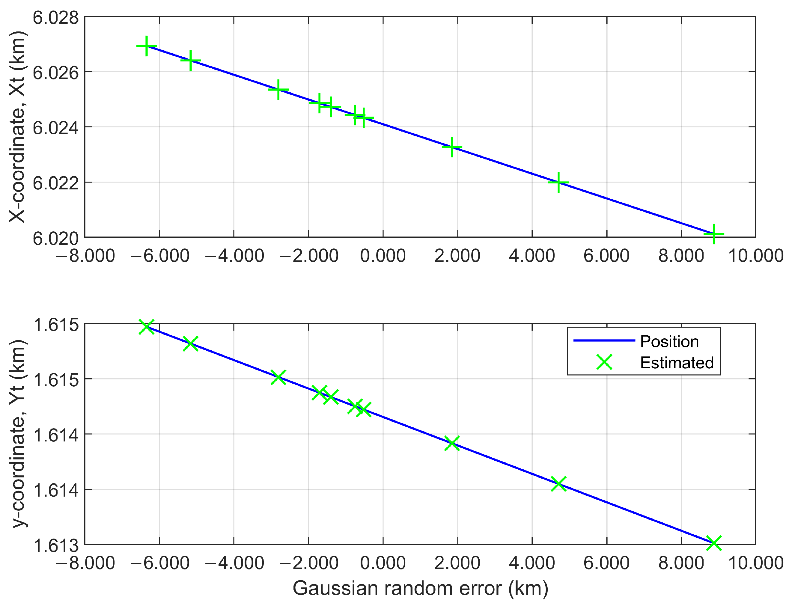
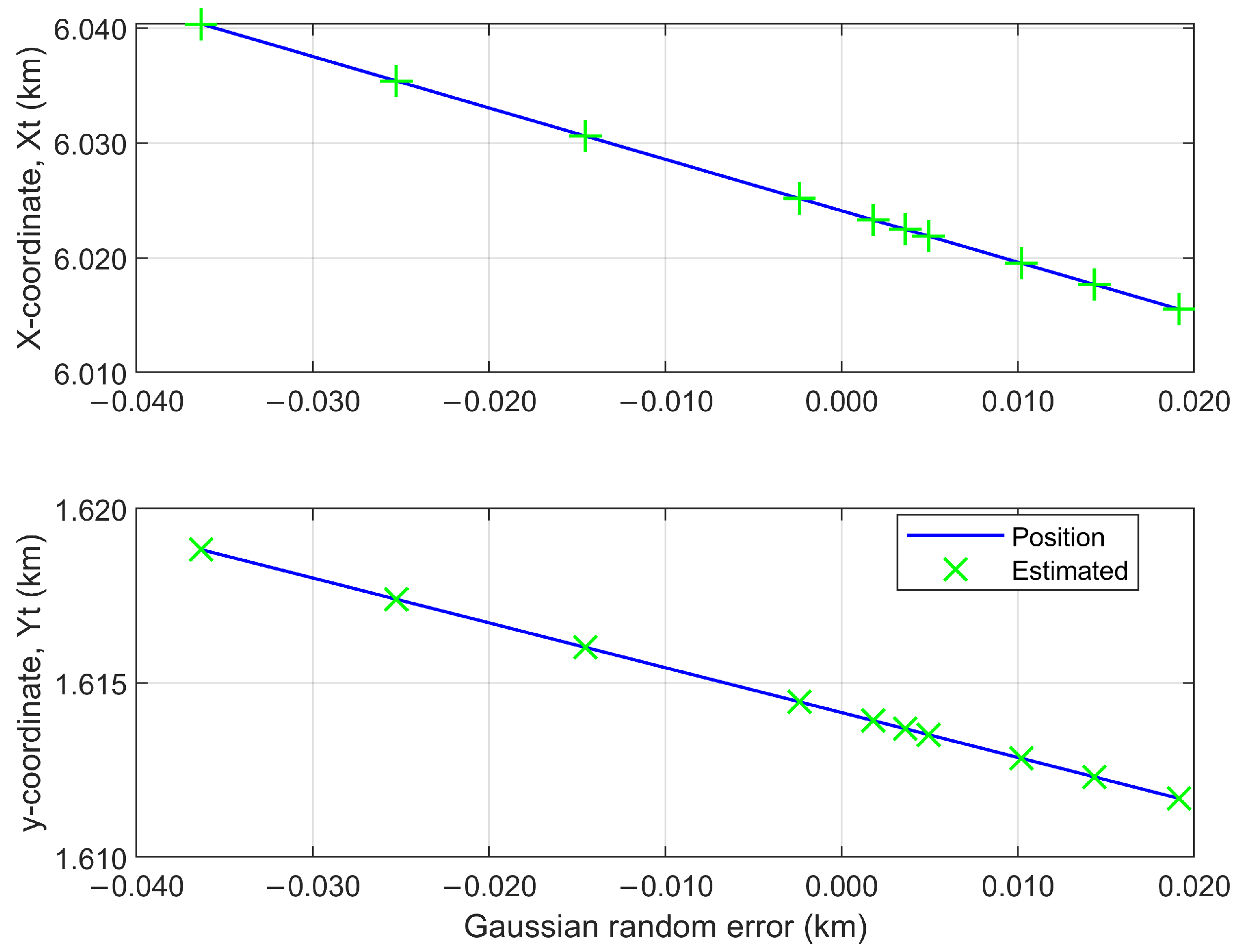
To test the accuracy of the algorithm, we performed additional simulations based on target-1 as a randomly selected case. In this scenario, the same two additive zero-mean Gaussian random errors $N(0,{\sigma }^2)$ with the same standard deviations ${\mathsf{\sigma }}_{\mathrm{d}}=6 \mathrm{m} \mathrm{a}\mathrm{n}\mathrm{d} 15 \mathrm{m}$ were used to disturb the RD measurements. Then the target position was estimated based on ten random values of Gaussian error.

The results of the simulations with standard deviations ${\mathsf{\sigma }}_{\mathrm{d}}=6 \mathrm{m}$ and ${\mathsf{\sigma }}_{\mathrm{d}}=15 \mathrm{m}$ are shown in Figure 7 and Figure 8, respectively.

In Figure 7 and Figure 8, the blue lines describe the curve of the position versus the Gaussian errors, and the green marks (+) indicate the estimated positions in the x and y coordinates of the target using the algorithm. As we can see, in both figures, all ten values of the estimated position were set very nearly and located in a narrow space for both the x (from 6.020 to 6.027 km for Figure 7 and from 6.015 to 6.040 for Figure 8) and y (from 1.613 to 1.615 km for Figure 7 and from 1.611 to 1.619 for Figure 8) coordinates.

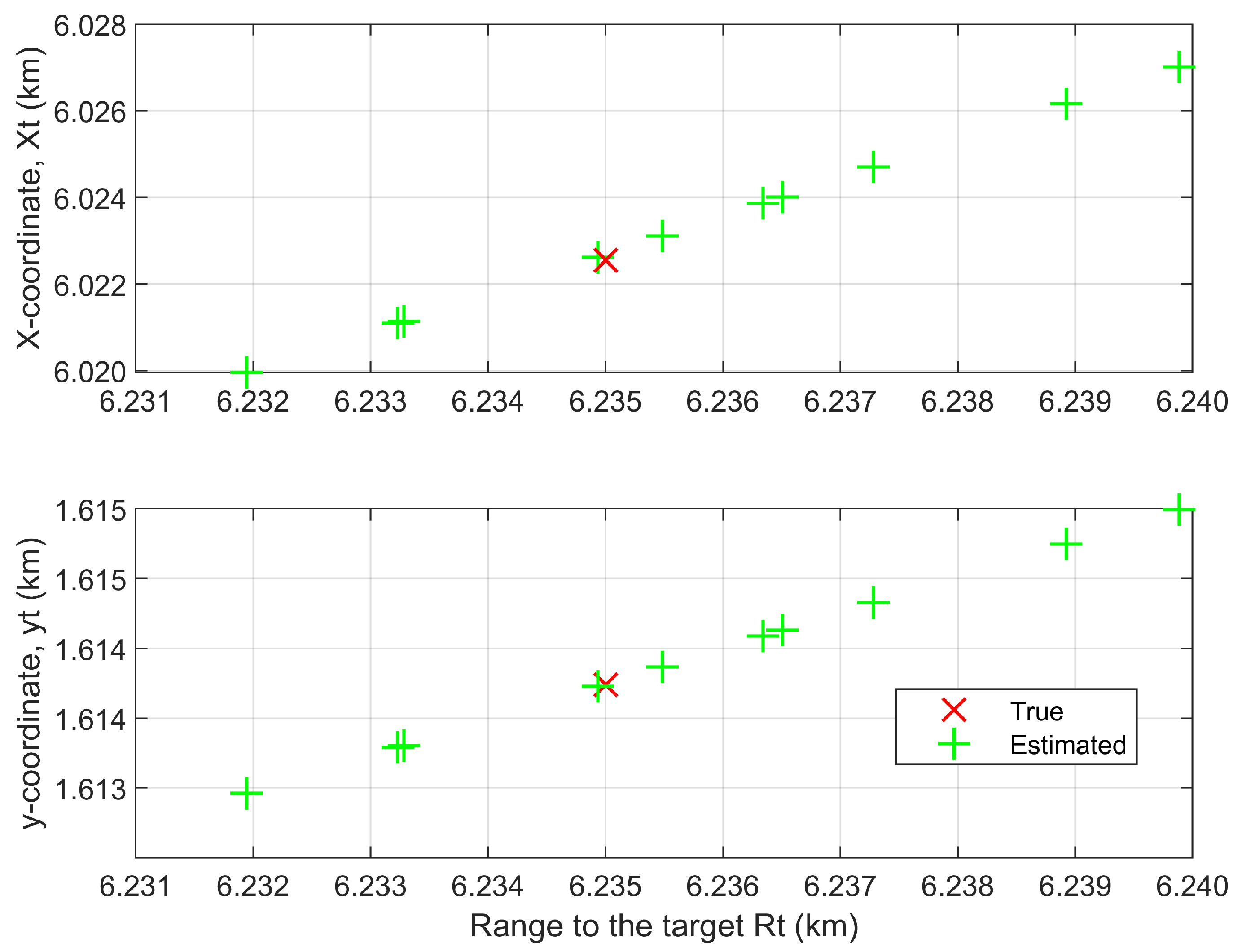
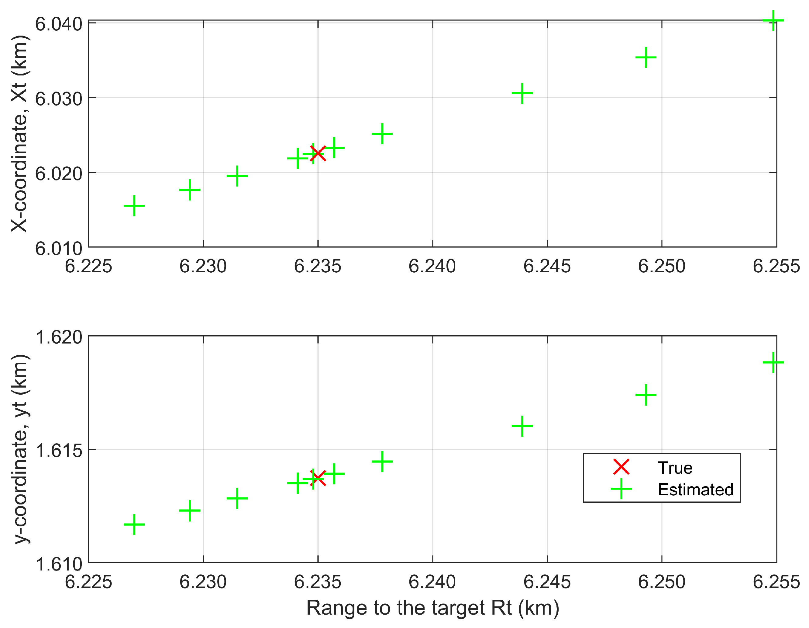
Figure 9 and Figure 10 display the locations of the x and y coordinates versus the range to the target $\mathrm{R}\mathrm{t}$ for ${\mathsf{\sigma }}_{\mathrm{d}}=6 \mathrm{m} \mathrm{a}\mathrm{n}\mathrm{d} 15 \mathrm{m}$, respectively. In the two figures, usually the green mark (+) indicates the estimated ten positions in the x and y coordinates of the target according to the ten values of $\mathrm{R}\mathrm{t}$, which correspond to the ten values of the Gaussian errors using the algorithm. The red marks (x) indicate the true positions in the x and y coordinates of the target (values in Table 1). The error between these ten estimated positions to locate the true x and y coordinates for the two cases of Gaussian errors was found to be ${\mathsf{\sigma }}_{\mathrm{x}}=2.26 \mathrm{m}$ and ${\mathsf{\sigma }}_{\mathrm{y}}=0.65 \mathrm{m}$ for ${\mathsf{\sigma }}_{\mathrm{d}}=6 \mathrm{m},$ and ${\mathsf{\sigma }}_{\mathrm{x}}=7.93 \mathrm{m}$ and ${\mathsf{\sigma }}_{\mathrm{y}}=2.28 \mathrm{m}$ for ${\mathsf{\sigma }}_{\mathrm{d}}=15 \mathrm{m}$.

Furthermore, for more investigation into the theoretical accuracy in position estimation using this method, the simulations were conducted 1000 times for each target to estimate the true position based on the same two standard deviations. In these scenarios, the results of the accuracy in the x and y coordinates are listed in

Table 3. The estimation accuracy of the algorithm with ${\mathsf{\sigma }}_{\mathrm{d}}=6 \mathrm{m}$.

Target No.	${\mathsf{\sigma }}_{\mathbf{x}}\left(\mathbf{m}\right)$	${\mathsf{\sigma }}_{\mathbf{y}}\left(\mathbf{m}\right)$
1	2.65	0.76
2	2.60	0.91
3	2.57	1.06
4	1.30	2.52

and

Table 4. The estimation accuracy of the algorithm with ${\mathsf{\sigma }}_{\mathrm{d}}=15 \mathrm{m}$.

Target No.	${\mathsf{\sigma }}_{\mathbf{x}}\left(\mathbf{m}\right)$	${\mathsf{\sigma }}_{\mathbf{y}}\left(\mathbf{m}\right)$
1	6.65	1.91
2	6.62	2.31
3	6.46	2.66
4	3.21	6.20

. It can be seen from the two tables that the small errors in the RD measurements of the target provide small errors in the accuracy of the algorithm, and vice versa. Consequently, these lower errors in both the x and y coordinates lead to locating the estimated positions in the vicinity of the true target’s position.

We can see from the numerical results regarding the target localization accuracy in previous scenarios for both the estimated target position and target-reference receiver range that the algorithm provided accurate estimated results for the two different errors. This accuracy means the RD measurements of these targets were typically measured precisely.

These results confirm that the method is valid for target localization as well as the estimation of the target-reference receiver range ${\mathrm{R}}_{\mathrm{t}}$ even for different RD errors, and its accuracy depends on the RD measurements.

6. Discussion

Referring to the theoretical study and performance of the method in the simulation results, in this area we summarized a short discussion of some points based on the proposed approach and the considered case study, which can be listed as follows:

−

The derivation of the approach was based on a pentagram array with a fixed number of receivers (N + 1 = 10).

−

The receivers were distributed only in two subspaces.

−

The receivers’ positions were spaced by a relatively far distances.

−

The case study assumed only a far-spaced situation for both receivers and targets under two Gaussian random errors with standard deviations σ = 6 and 15 m.

−

The accuracy of the algorithm depends on the errors in the RD measurements (small errors provide good accuracy).

−

Localization obtained by (18) based on finding the value of R_t can be compared with that of the SX and SI methods.

−

For extending the approach to an arbitrary array geometry and number (N) of receivers, the theoretical and mathematical formulation of the approach must be recomputed using the selected array or receiver’s configuration.

7. Conclusions and Future Works

This paper proposes a simple method for target localization using range difference (RD) measurements from $\mathrm{N}+1$ receivers ($\mathrm{N}=9$). The approach was derived using a closed-form solution from RDs based on a pentagram array. It is presented as an alternative method to avoid the contradiction between the two well-known TDOA system methods (SX and SI). In [25], SI performed better than SX; conversely, in [4], SX performed better compared to SI.

Using numerical analysis based on an assumption-based passive radar scenario, the performance of the approach was investigated for different targets and RD measurements using two Gaussian random errors with zero mean and standard deviations $\mathsf{\sigma }=6 \mathrm{m} \mathrm{a}\mathrm{n}\mathrm{d} 15 \mathrm{m}$ according to ionosphedriec time delays of 20 and 50 nsec, respectively. The well-conducted analysis provided good accuracy for target localization results. Additionally, the accuracy of the estimated target positions in the x and y coordinates was calculated, which essentially depends on the accuracy of the RD measurements. The small errors in the RD measurements lead to the good accuracy of the approach.

As a consequence, the new approach is suitable for 2D localization in the considered case (passive radar localization). Its application only for 2D target localization refers to the particular placement of the receivers in the considered array.

The method is fast due to its low computational burden, which is based on a closed-form equation and is easily executed. Additionally, it can be used for numerous targets by dealing with everyone in a single scenario.

In the future, we will focus our studies on the application of the proposed localization approach in particular cases, such as those involving large-area distributed transmitters, one receiver and target, real-life experiments, practical applications, and target tracking problems.