Separation of Multicomponent Micro-Doppler Signal with Missing Samples

Abstract

The problem of separating multicomponent micro-Doppler (m-D) signals is common in the field of radar signal processing. In some implementations, it is necessary to separate the multicomponent m-D signal that contains missing samples. To address this issue, an optimization model has been developed to recover and decompose multicomponent m-D signals with missing samples. To solve the underlying optimization problem, a two-algorithm-based alternate iteration framework is proposed. This method uses three techniques—the null space property, ridge regression method, and matching pursuit principle—to estimate the individual component, complex-valued differential operator, and regularization parameter. Finally, as shown by both simulation and measured data processing results, the proposed method can accurately separate the multicomponent m-D signal from incomplete data.

1. Introduction

Micro-motion refers to small movements, such as vibrations and rotations of the target or target parts, which are excluded from the translation of the main body [1]. A micro-motion target produces frequency modulation on the radar echoes, causing a multicomponent micro-Doppler (m-D) signal. Multicomponent m-D signal decomposition has received extensive attention in microwave remote sensing due to the ability of m-D signal components to exhibit more detailed target characteristics, such as the precession frequency of artificial metal targets or the length of the rotating blades [2].

As the instantaneous frequency (IF) of the spinning scatterer echo can be approximated using a sinusoidal function, several multicomponent m-D signal decomposition methods based on sinusoidal frequency modulated (SFM) signal matching have been proposed. Peng et al. [3] proposed the sinusoidal frequency modulation Fourier transform (SFMFT) based on SFM signal space for multicomponent SFM signal decomposition. Furthermore, by introducing the K-resolution parameter on the Bessel function basis, researchers in [4] proposed the sinusoidal frequency modulation Fourier–Bessel (SFMFB) transform to separate multicomponent m-D signals. Based on point-line duality, the inverse Radon transform, Hough transform, and their extension methods are applied to estimate the parameters of the SFM signal and extract the micro-motion features [5,6,7,8]. However, the above methods are not applicable when the pattern of IF is more complex or irregular.

For micro-Doppler signal components with irregular IF, the Hilbert–Huang transform (HHT) and the variational modal decomposition (VMD) method are proposed for signal decomposition, which derives from adaptive filtering methods [9]. Since most of the radar data are complex signals, extended VMD methods such as complex-valued empirical mode decomposition (CVEMD) and bivariate variational mode decomposition are used to separate the echo signals of the main body and the micro-motion parts of the target [10,11]. The decomposition result of measured data has demonstrated that these methods perform well with nonstationary signals. However, these methods do not fit for decomposing multicomponent signals with the overlapping frequency spectrum. Although some variants of VMD have been successfully proposed for extracting multicomponent m-D signals containing crossed modes, such as the short-time variational modal decomposition (STVMD) [12] and variational nonlinear chirp mode decomposition (VNCMD) [13], they both require the number of components as a priori. Based on the recursive decomposition scheme, the operator-based signal separation (OSS) method [14,15] and adaptive chirp mode pursuit (ACMP) [16] have been used in multicomponent signal decomposition without the number of components in advance. In addition, signal separation methods based on fractional Fourier transform FRFT [17], time-scale frequency-modulation slope operator [18], and chirplet transform [19] have been successively used to extract the frequency-changing curves of nonstationary signals that are concerned with the time-frequency domain. These methods estimate the instantaneous frequency of each component signal by searching the parameters of the multicomponent signal from the three-dimensional space of time, frequency, and frequency modulation slope.

In real-world scenarios, the radar data of micro-motion targets may be incomplete with randomly missing samples due to strong interference. When echoes of micro-motion targets are corrupted with only randomly positioned samples due to interference or sensor failure, the state-of-art radar imaging techniques become invalid. Under this circumstance: (1) In the situation of long-range, the micro-motion target with a small radar cross section (i.e., low signal-to-noise (SNR)) may not be extracted from the receiver noise. (2) Some samples must be discarded during the strong interference of the micro-motion target echo; otherwise, sensor failure and outliers prevent effective observation of the data samples [20]. To recover target features from incomplete data, methods based on over-complete parameters or time-frequency (T-F) dictionaries have been proposed. However, the above methods do not achieve effective separation of multicomponent signals [21,22,23,24,25].

In this paper, inspired by the OSS method, an alternate iterative optimization framework is constructed for multicomponent m-D signal with missing samples decomposition and reconstruction. The specific contributions of this paper are as follows:

(1)

We propose two algorithms to solve the alternate iteration framework. The first algorithm uses the iteratively reweighted least squares (IRLS), Tikhonov regularization, and the matching pursuit principle to extract signal components, regularize the complex-valued differential (CD) operator, and calculate the optimization parameters, respectively.

(2)

To improve the accuracy of extracting signal components, the second algorithm employs the alternating direction method of multipliers (ADMM), iterative Tikhonov regularization, and the fixed-point iteration principle to extract signal components, regularize the CD operator, and calculate the optimization parameters, respectively.

(3)

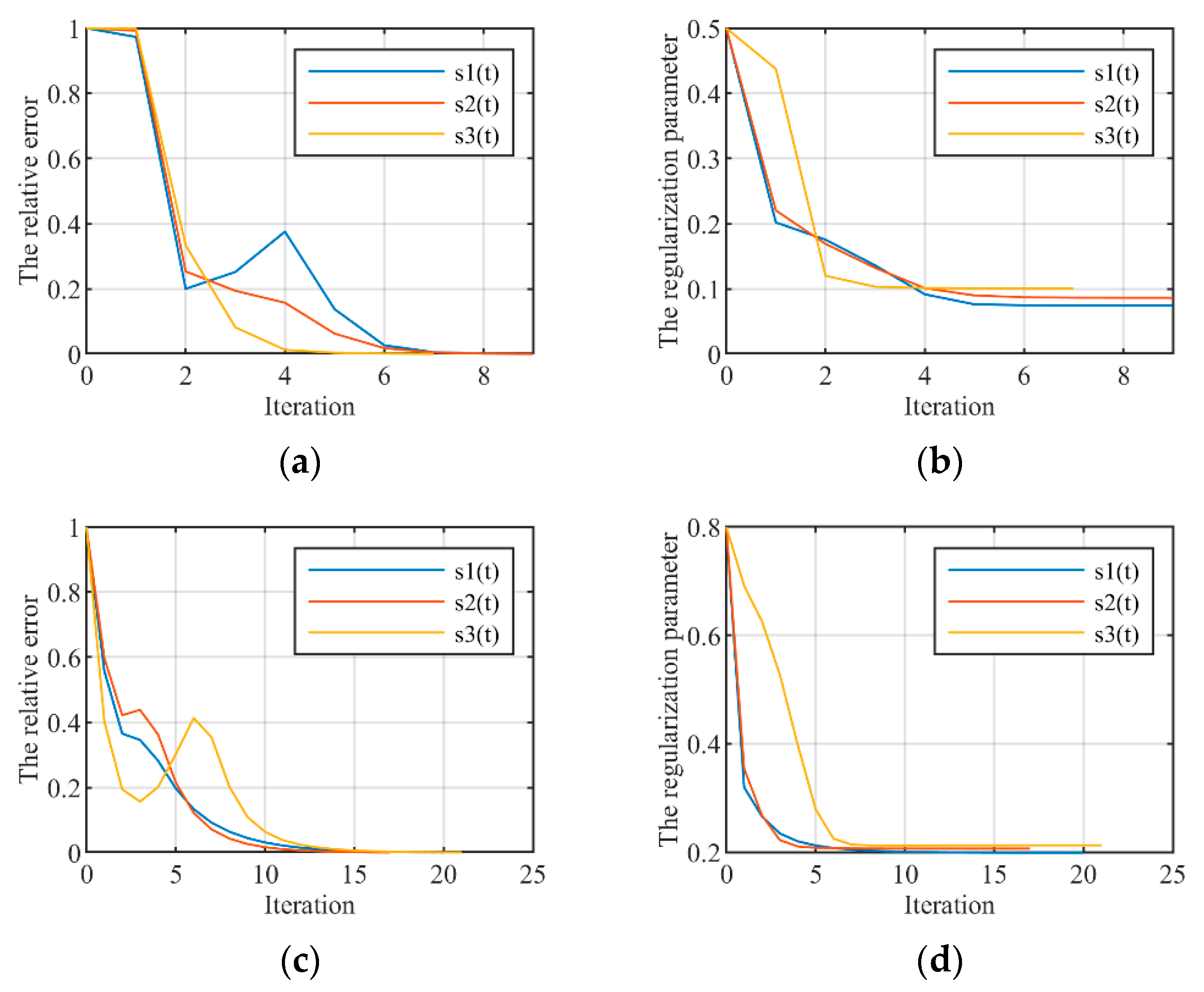
Furthermore, an adaptive parameter updating method is proposed for iterative Tikhonov regularization.

The rest of this paper is organized as follows: The signal model and problem formulation are described in Section 2. Section 3 proposes a decomposition method for multicomponent m-D signals with missing samples. Section 4 illustrates the effectiveness of the proposed method by simulated and measured signals. Section 5 is a discussion and Section 6 is a conclusion.

2. Signal Model and Problem Formulation

In a high-frequency electromagnetic regime, the target can be constructed by a point scattering model [23]. The micro-motion target echo can be regarded as a multicomponent m-D signal. The multicomponent m-D signal with missing samples can be expressed as

$$s(t)={\displaystyle \sum _{k=1}^{K}p(t)s_k(t)+\eta (t)}={\displaystyle \sum _{k=1}^{K}p(t)a_k(t)\exp \left(j\frac{4\pi }{\lambda }{R}_k(t)\right)+}\eta (t)$$

(1)

where $K$ represents the number of scatterers; $p\left(t\right)$ stands for missing samples, $p\left(t\right)\subset \left\{0,1\right\}$. $j^2=-1$. $a_k\left(t\right)>0$ indicates the instantaneous amplitude (IA). $R(t)$ denotes the instantaneous range between the radar and the k-th scatterer. ${\phi }_k(t)=4\pi R_k(t)/\lambda$ stands for instantaneous phase. $s_k(t)$ is the individual component. $f_k(t)={{\phi }^{\prime }}_k(t)/2\pi$ stands for IF. $\eta (t)$ is the Gaussian white noise. The IA and IF of a signal change more slowly than its phase function and $\left|{a^{\prime }}_k(t)\right|,\left|{f^{\prime }}_k\left(t\right)\right|\ll \left|f_k\left(t\right)\right|$.

$\mathsf{\Omega }(\cdot )$ is defined as a second-order differential operator, which is $\mathsf{\Omega }(s_k(t))=d^2{s}_k(t)/d{t}^2$. The second-order differential of individual components can be expressed as

$$\mathsf{\Omega }\left(s_k\left(t\right)\right)={\alpha }_k\left(t\right)s_k\left(t\right)$$

(2)

with

$${\alpha }_k\left(t\right)=\frac{{a^{″}}_k\left(t\right)}{a_k\left(t\right)}-{\left({{\phi }^{\prime }}_k\left(t\right)\right)}^2+j\left(\frac{2{a^{\prime }}_k\left(t\right){{\phi }^{\prime }}_k\left(t\right)}{a_k\left(t\right)}+{{\phi }^{″}}_k\left(t\right)\right)$$

(3)

where $\mathsf{\Omega }-{\alpha }_k$ is set to be the null space operator $T_k$, and $T_k\left(s_k\left(t\right)\right)=0$. It means that $T_k$ has the function of individual component decomposition. Based on the ability of $T_k$ to decompose individual components and the sparsity of individual components in the T-F domain, the decomposition of individual components $s_k\left(t\right)$ with missing samples can be described as an optimization problem in (4),

$$\underset{{\mathsf{\alpha }}_k,{\mathbf{s}}_k}{\min }{‖{\mathbf{T}}_k{\mathbf{s}}_k‖}_2^2+\lambda {‖\mathbf{s}-\mathbf{P}{\mathbf{s}}_k‖}_2^2+\upsilon {‖\mathbf{W}{\mathbf{s}}_k‖}_1+\mu {‖\mathsf{\Omega }{\mathsf{\alpha }}_k‖}_2^2$$

(4)

in which $\mathsf{\Omega }$ can be written as

$$\mathsf{\Omega }=\left[\begin{array}{ccccccc}1& 1& 0& 0& 0& \cdots & 0\\ 1& -2& 1& 0& 0& \cdots & 0\\ ⋮& \ddots & \ddots & \ddots & \ddots & \ddots & ⋮\\ 0& \cdots & 0& 0& 1& -2& 1\\ 0& \cdots & 0& 0& 0& 1& -1\end{array}\right]$$

(5)

where $\mathbf{s}={\left[s\left(t_1\right)\dots s\left(t_n\right)\dots s\left(t_N\right)\right]}^{\mathrm{T}}$ stands for m-D signal with missing samples, ${\mathbf{s}}_k={\left[s_k\left(t_1\right)\dots s_k\left(t_n\right)\dots s_k\left(t_N\right)\right]}^{\mathrm{T}}$ stands for the k-th component, and $n\in [1,N]$, ${\left(\cdot \right)}^{\mathrm{T}}$ denotes the transpose of matrix. ${\mathbf{T}}_k=\mathsf{\Omega }-{\mathsf{\alpha }}_k$, $\mathsf{\Omega }$ is a modified second-order differential operator and ${\mathsf{\alpha }}_k=\mathrm{diag}\left\{{\alpha }_k\left(t_1\right)\dots {\alpha }_k\left(t_n\right)\dots {\alpha }_k\left(t_N\right)\right\}$, $\mathrm{diag}\{\cdot \}$ denotes a diagonalization operator. $\mathbf{W}\in {ℂ}^{MN\times N}$ is a short-time Fourier transform matrix, $M={N/m}_s$ and $m_s$ stand for the step of the sliding window. $\mathbf{W}=\mathbf{HQ}$, $\mathbf{H}=\mathrm{diag}\{\mathbf{Y},\dots \mathbf{Y}\}$ and $\mathbf{H}\in {ℂ}^{MN\times MN}$. $\mathbf{Y}$ stands for the Fourier transform matrix. $\mathbf{Q}=[{\mathbf{B}}^1\dots {\mathbf{B}}^m\dots {\mathbf{B}}^M{]}^{\mathrm{T}}$ is the sliding window matrix, ${\mathbf{B}}^m=\mathrm{diag}\{b^m(1),\dots b^m(n),\dots b^m(N)\}$ represents the m-th window matrix, and ${\mathbf{B}}^m\in {ℝ}^{N\times N}$ [25]. $\mathbf{P}$ is an incomplete sampling diagonal matrix, which consists of $p\left(t\right)$. The first term denotes the extraction of component ${\mathbf{s}}_k$ by the null space operator ${\mathbf{T}}_k$. The second term is used to regularize the residual signal $\mathbf{s}-\mathbf{P}{\mathbf{s}}_k$. $\upsilon$, $\lambda$ and $\mu$ are regularization parameters. $\upsilon$ denotes the regularization parameter. In general, the larger the value of $\upsilon$, the sparser the result of the reconstruction. It is reasonable to assume that ${\mathbf{s}}_k$ is sparse in the time-frequency (TF) domain, so the third term represents sparse prior of $\mathbf{W}{\mathbf{s}}_k$. The parameter $\lambda$ determines the energy of ${\mathbf{s}}_k$ in the null space. The fourth term indicates the regularization of the CD operator ${\mathsf{\alpha }}_k$ and ensures the smoothness of the operator. ${‖\cdot ‖}_1$ and ${‖\cdot ‖}_2$ stand for L₁-norm and L₂-norm, respectively.

3. Algorithm Design

In Section 2, the decomposition of incomplete multicomponent m-D signals has been formulated as an optimization problem. In that section, two methods are proposed for solving the problem. As the CD operator is not known as a priori, the problem described in (4) needs to be split into two optimization problems solving the signal components and CD operator separately. As shown in Algorithm 1, the problem constructed by Problem (4) can be approximately solved by solving Problem (6) and Problem (7) alternately.

Algorithm 1 The framework of the proposed method

Initialization $i=0$, ${\lambda }^{\left(i\right)}$$, {\upsilon }^{\left(i\right)}$, $\mu$, ${\mathsf{\alpha }}_k^{\left(i\right)}\left({\mathbf{T}}_k^{\left(i\right)}=\mathsf{\Omega }-{\mathsf{\alpha }}_k^{\left(i\right)}\right)$, ${\mathbf{s}}_k^{\left(i\right)}$, $\xi$;

Repeat

$\mathrm{Given} {\mathsf{\alpha }}_k^{\left(i\right)}$

$${\mathbf{s}}_k^{\left(i+1\right)}=\arg \underset{{\mathbf{s}}_k}{\min }{‖{\mathbf{T}}_k{\mathbf{s}}_k‖}_2^2+\lambda {‖\mathbf{s}-\mathbf{P}{\mathbf{s}}_k‖}_2^2+\upsilon {‖\mathbf{W}{\mathbf{s}}_k‖}_1$$ (6)

$\mathrm{Given} {\mathbf{s}}_k^{\left(i\right)}$

$${\mathsf{\alpha }}_k^{\left(i+1\right)}=\arg \underset{{\mathsf{\alpha }}_k}{\min }{‖{\mathbf{T}}_k{\mathbf{s}}_k‖}_2^2+\mu {‖\mathsf{\Omega }{\mathsf{\alpha }}_k‖}_2^2$$ (7)

Update regularization parameters $\lambda$ and $\upsilon$

Until ${\displaystyle {\sum }_k{‖{\mathbf{s}}_k^{\left(i+1\right)}-{\mathbf{s}}_k^{\left(i\right)}‖}_2^2/{‖{\mathbf{s}}_k^{\left(i\right)}‖}_2^2<\xi }$

3.1. IRLS-Based Algorithm

The problem described in (6) can be regarded as a basis pursuit or variable splitting problem, which can be addressed by interior-point methods [24] or alternating direction methods of multipliers [26], respectively. In order to take advantage of the automatic parameter updating of the proposed approach, the problem is solved by the IRLS algorithm here, and Equation (6) can be reformulated as

$${\mathbf{s}}_k=\arg \underset{{\mathbf{s}}_k}{\min }{‖{\mathbf{T}}_k{\mathbf{s}}_k‖}_2^2+\lambda {‖\mathbf{s}-\mathbf{P}{\mathbf{s}}_k‖}_2^2+\upsilon {\mathbf{s}}_k^{\mathbf{H}}{\mathbf{W}}^{\mathbf{H}}{\mathbf{R}}^{-1}\mathbf{W}{\mathbf{s}}_k$$

(8)

where $\mathbf{R}=\mathrm{diag}\{\left|\mathbf{W}{\mathbf{s}}_k\right|\}$ and L₁-norm ${‖\mathbf{W}{\mathbf{s}}_k‖}_1$ can be viewed as an adaptively weighted version of the squared L₂-norm ${‖\mathbf{QW}{\mathbf{s}}_k‖}_2^2$. The problem given in (8) can be reformulated as

$${\mathbf{s}}_k=\arg \underset{{\mathbf{s}}_k^{\left(i\right)}}{\min }{‖{\mathbf{T}}_k{\mathbf{s}}_k‖}_2^2+\lambda {‖\mathbf{s}-\mathbf{P}{\mathbf{s}}_k‖}_2^2+\upsilon {‖\mathbf{QW}{\mathbf{s}}_k‖}_2^2$$

(9)

where ${\mathbf{R}}^{-1}={\mathbf{Q}}^T\mathbf{Q}$. By using IRLS, the solution to Problem (9) can be formulated as

$${\mathbf{s}}_k^{\left(i+1\right)}={\left(2{\mathbf{T}}_k^{\mathbf{H}}\mathbf{T}+2\lambda {\mathbf{P}}^{\mathbf{T}}\mathbf{P}+2\upsilon {\mathbf{W}}^{\mathbf{H}}{\mathbf{Q}}^{\mathbf{H}}\mathbf{QW}\right)}^{-1}2\lambda \mathbf{Ps}$$

(10)

For the problem in Equation (7), let ${\mathsf{\alpha }}_k$ be the vector that ${\mathsf{\theta }}_k=\mathrm{diag}\left\{{\mathsf{\alpha }}_k\right\}$, and the Equation (7) can be rewritten as

$$\mathsf{\Gamma }({\mathsf{\theta }}_k)={‖\mathsf{\Omega }{\mathbf{s}}_k-{\mathsf{\Xi }}_k{\mathsf{\theta }}_k‖}_2^2+\mu {‖\mathsf{\Omega }{\mathsf{\theta }}_k‖}_2^2$$

(11)

where ${\mathsf{\Xi }}_k=\mathrm{diag}\left\{{\mathbf{s}}_k^{i+1}\right\}$. The Equation (11) can be regarded as Tikhonov regularization. By taking the partial derivative of $\mathsf{\Gamma }(\cdot )$ with respect to ${\mathsf{\theta }}_k$ and making the result being zero, the problem described in Equation (11) can be solved as

$${\mathsf{\theta }}_k^{\left(i+1\right)}={\left({\mathsf{\Xi }}_k^{\mathbf{H}}{\mathsf{\Xi }}_k+\mu {\mathsf{\Omega }}^{\mathbf{T}}\mathsf{\Omega }\right)}^{-1}{\mathsf{\Xi }}_k^{\mathbf{H}}\mathsf{\Omega }{\mathbf{s}}_k^{\left(i+1\right)}$$

(12)

Based on the matching pursuit principle, the individual component ${\mathbf{s}}_k$ and residual signal $\mathbf{s}-{\mathbf{s}}_k$ are approximately mutually orthogonal, i.e.,

$${\left({\mathbf{s}}_k\right)}^{\mathbf{H}}\left(\mathbf{s}-{\mathbf{s}}_k\right)=0$$

(13)

The parameter $\lambda$ determines the amount of information about the residual signal. According to Equations (10) and (13), the parameters $\lambda$ can be calculated by

$$\frac{{\mathbf{s}}^{\mathbf{H}}\left(\mathbf{V}\left({\mathbf{T}}_k,\mathbf{Q},\upsilon ,\lambda \right)\right)\mathbf{s}}{\lambda {\mathbf{s}}^{\mathbf{H}}{\left(\mathbf{V}\left({\mathbf{T}}_k,\mathbf{Q},\upsilon ,\lambda \right)\right)}^{\mathbf{H}}\left(\mathbf{V}\left({\mathbf{T}}_k,\mathbf{Q},\upsilon ,\lambda \right)\right)\mathbf{s}}=1$$

(14)

with

$$\mathbf{V}\left({\mathbf{T}}_k,\mathbf{Q},\upsilon ,\lambda \right)=\left(2{\mathbf{T}}_k^{\mathbf{H}}{\mathbf{T}}_k+\right.2\lambda {\mathbf{P}}^{\mathbf{T}}\mathbf{P}{\left.+2\upsilon {\mathbf{W}}^{\mathbf{T}}{\mathbf{Q}}^{\mathbf{T}}\mathbf{QW}\right)}^{-1}\mathbf{P}$$

(15)

According to Equation (14), the value of $\lambda$ can be estimated by

$${\lambda }^{\left(i+1\right)}=\frac{{\mathbf{s}}^{\mathrm{H}}\left(\mathbf{V}\left({\mathbf{T}}_k,\mathbf{Q},{\upsilon }^i,{\lambda }^i\right)\right)\mathbf{s}}{{\mathbf{s}}^{\mathrm{H}}{\left(\mathbf{V}\left({\mathbf{T}}_k,\mathbf{Q},{\upsilon }^i,{\lambda }^i\right)\right)}^{\mathrm{H}}\left(\mathbf{V}\left({\mathbf{T}}_k,\mathbf{Q},{\upsilon }^i,{\lambda }^i\right)\right)\mathbf{s}}$$

(16)

The IRLS-based algorithm is shown in Algorithm 2, which consists of two loops. The first loop is used to update the residue signal and the second loop is used to extract the component ${\mathbf{s}}_k$. The parameter $\xi$ is the relative error, $\eta$ is the stopping threshold, $\mathbf{r}$ is the residue signal, and ${\mathbf{r}}^{\left(0\right)}=\mathbf{s}$. The parameter $\mu$ determines the smoothness of ${\mathsf{\alpha }}_k$. Since $\mu$ is insensitive to ${\mathsf{\alpha }}_k$, it is set to be a fixed value. The initialization of ${\mathsf{\alpha }}_k$ can be obtained by ${\mathsf{\theta }}_k^{\left(1\right)}={({({\mathbf{R}}^{\left(m\right)})}^{\mathrm{H}}{\mathbf{R}}^{\left(m\right)}+\mu {\mathsf{\Omega }}^{\mathrm{T}}\mathsf{\Omega })}^{-1}{({\mathbf{R}}^{\left(m\right)})}^{\mathrm{H}}\mathsf{\Omega }{\mathbf{r}}^{\left(m\right)}$, where ${\mathbf{R}}^{\left(m\right)}=\mathrm{diag}\{{\mathbf{r}}^{\left(m\right)}\}$,${\mathsf{\theta }}_k^{(1)}=\mathrm{diag}\{{\mathsf{\alpha }}_k^{(1)}\}$.

Algorithm 2 IRLS-based algorithm

Input: $i=0$, $m=0$, ${\lambda }^{\left(i\right)}$$\upsilon$, $\mu$, ${\mathbf{s}}_k^{\left(i\right)}$$\eta$, $\xi$.

$\mathbf{while} {‖{\mathbf{r}}^{\left(m\right)}‖}_2^2/{‖\mathbf{s}‖}_2^2>\eta$ do

Initialization ${\mathsf{\alpha }}_k^{\left(i\right)}\left({\mathbf{T}}_k^{\left(i\right)}=\mathsf{\Omega }-{\mathsf{\alpha }}_k^{\left(i\right)}\right)$

while ${‖{\mathbf{s}}_k^{\left(i+1\right)}-{\mathbf{s}}_k^{\left(i\right)}‖}_2^2/{‖{\mathbf{s}}_k^{\left(i\right)}‖}_2^2>\xi$ do

$i\leftarrow i+1$

${\mathbf{s}}_k^{\left(i+1\right)}={\left(2{\mathbf{T}}_k^{\mathrm{H}}\mathbf{T}+2\lambda {\mathbf{P}}^{\mathrm{T}}\mathbf{P}+2\upsilon {\mathbf{W}}^{\mathrm{H}}{\mathbf{Q}}^{\mathrm{H}}\mathbf{QW}\right)}^{-1}2\lambda \mathbf{P}{\mathbf{r}}^{\left(m\right)}$

$\mathbf{V}\left({\mathbf{T}}_k,\mathbf{Q},\upsilon ,\lambda \right)=\left(2{\mathbf{T}}_k^{\mathrm{H}}{\mathbf{T}}_k+\right.2\lambda {\mathbf{P}}^{\mathrm{T}}\mathbf{P}{\left.+2{\mathbf{W}}^{\mathrm{T}}{\mathbf{Q}}^{\mathrm{T}}\mathbf{QW}\right)}^{-1}\mathbf{P}$

${\lambda }^{\left(i+1\right)}=\frac{{\left({\mathbf{r}}^{\left(m\right)}\right)}^{\mathrm{H}}\left(\mathbf{V}\left({\mathbf{T}}_k,\mathbf{Q},{\upsilon }^i,{\lambda }^i\right)\right){\mathbf{r}}^{\left(m\right)}}{{\left({\mathbf{r}}^{\left(m\right)}\right)}^{\mathrm{H}}{\left(\mathbf{V}\left({\mathbf{T}}_k,\mathbf{Q},{\upsilon }^i,{\lambda }^i\right)\right)}^{\mathrm{H}}\left(\mathbf{V}\left({\mathbf{T}}_k,\mathbf{Q},{\upsilon }^i,{\lambda }^i\right)\right){\mathbf{r}}^{\left(m\right)}}$

${\mathsf{\theta }}_k^{\left(i+1\right)}={\left({\mathsf{\Xi }}_k^{\mathrm{H}}{\mathsf{\Xi }}_k+\mu {\mathsf{\Omega }}^{\mathbf{T}}\mathsf{\Omega }\right)}^{-1}{\mathsf{\Xi }}_k^{\mathbf{H}}\mathsf{\Omega }{\mathbf{s}}_k^{\left(i+1\right)}$

end while

update the residue signal ${\mathbf{r}}^{\left(m\right)}=\mathbf{s}-{\displaystyle \sum _{k=1}^m{\mathbf{s}}_k}$

$m\leftarrow m+1$

end while

Output: reconstructed components ${\mathbf{s}}_k$

3.2. ADMM-Based Algorithm

The variable splitting method [26] is introduced to solve the problem described in (6), and it can be rewritten as

$$\underset{{\mathbf{f}}_k,{\mathbf{s}}_k}{\min }{f}_1({\mathbf{f}}_k)+f_2({\mathbf{s}}_k)\hspace{1em}s.t.\hspace{0.33em} {\mathbf{f}}_k=\mathbf{W}{\mathbf{s}}_k$$

(17)

with

$$f_1({\mathbf{f}}_k)=\upsilon {‖{\mathbf{f}}_k‖}_1$$

(18)

$$f_2({\mathbf{s}}_k)={‖{\mathbf{T}}_k{\mathbf{s}}_k‖}_2^2+\lambda {‖\mathbf{s}-\mathbf{P}{\mathbf{s}}_k‖}_2^2$$

(19)

where ${\mathbf{f}}_k$ stands for time-frequency representation (TFR) of ${\mathbf{s}}_k$. The variable splitting problem defined in (17) can be solved by the simplex algorithm based on subproblems, which are more complicated compared with ADMM. Therefore, the problem (17) is solved by ADMM [26]. The augmented Lagrange function of (17) can be expressed as

$$\mathcal{L}({\mathbf{s}}_k,{\mathbf{f}}_k,\mathbf{u})={‖{\mathbf{T}}_k{\mathbf{s}}_k‖}_2^2+\lambda {‖\mathbf{s}-\mathbf{P}{\mathbf{s}}_k‖}_2^2+\upsilon {‖\mathbf{W}{\mathbf{s}}_k‖}_1+{〈\mathbf{u},\mathbf{W}{\mathbf{s}}_k-{\mathbf{f}}_k〉}^{\mathbf{T}}+\frac{\rho }{2}{‖\mathbf{W}{\mathbf{s}}_k-{\mathbf{f}}_k‖}_2^2$$

(20)

where $\mathbf{u}$ stands for Lagrange multiplier, $\rho$ stands for penalty coefficient, and $〈\cdot ,\cdot 〉$ represents inner product operation. The Equation (20) can be reformulated as

$$\mathcal{L}({\mathbf{s}}_k,{\mathbf{f}}_k,\mathbf{u})={‖{\mathbf{T}}_k{\mathbf{s}}_k‖}_2^2+\lambda {‖\mathbf{s}-\mathbf{P}{\mathbf{s}}_k‖}_2^2+\upsilon {‖\mathbf{W}{\mathbf{s}}_k‖}_1+\frac{\rho }{2}{‖\mathbf{W}{\mathbf{s}}_k-{\mathbf{f}}_k+\frac{1}{\rho }\mathbf{u}‖}_2^2-\frac{1}{2\rho }{‖\mathbf{u}‖}_2^2$$

(21)

To estimate the single component ${\mathbf{s}}_k$, the objective function (21) can be rewritten as

$${\mathbf{s}}_k=\arg \underset{{\mathbf{s}}_k}{\min }||{\mathbf{T}}_k{\mathbf{s}}_k|{|}_2^2+\lambda ||\mathbf{s}-\mathbf{P}{\mathbf{s}}_k|{|}_2^2+\frac{\rho }{2}{‖\mathbf{W}{\mathbf{s}}_k-{\mathbf{f}}_k+\frac{1}{\rho }\mathbf{u}‖}_2^2$$

(22)

Finding the partial derivative with respect to ${\mathbf{s}}_k$ for Problem (22), i.e.,

$$\begin{array}{l}\frac{\partial }{\partial {\mathbf{s}}_k}\left\{{‖{\mathbf{T}}_k{\mathbf{s}}_k‖}_2^2+\lambda {‖\mathbf{s}-\mathbf{P}{\mathbf{s}}_k‖}_2^2+\frac{\rho }{2}{‖\mathbf{W}{\mathbf{s}}_k-{\mathbf{f}}_k+\frac{1}{\rho }\mathbf{u}‖}_2^2\right\}\\ =2{\mathbf{T}}_k^{\mathrm{H}}{\mathbf{T}}_k{\mathbf{s}}_k+2\lambda \left({\mathbf{P}}^{\mathrm{T}}\mathbf{P}{\mathbf{s}}_k-{\mathbf{P}}^{\mathrm{T}}\mathbf{s}\right)+\frac{\rho }{2}\left(2{\mathbf{W}}^{\mathrm{H}}\mathbf{W}{\mathbf{s}}_k-2{\mathbf{W}}^{\mathrm{H}}{\mathbf{f}}_k+\frac{2}{\rho }{\mathbf{W}}^{\mathrm{H}}\mathbf{u}\right)\end{array}$$

(23)

Let the value of Equation (23) be zero, then the solution to Problem (22) is

$${\mathbf{s}}_k^{\left(i+1\right)}={\left(2{\mathbf{T}}_k^{\mathrm{H}}{\mathbf{T}}_k+2\lambda {\mathbf{P}}^{\mathrm{T}}\mathbf{P}+\rho {\mathbf{W}}^{\mathrm{H}}\mathbf{W}\right)}^{-1}\left(2\lambda {\mathbf{P}}^{\mathrm{T}}\mathbf{s}+\rho {\mathbf{W}}^{\mathrm{H}}\left({\mathbf{f}}_k-\mathbf{u}\right)\right)$$

(24)

To estimate ${\mathbf{f}}_k$, the objective Function (21) can be rewritten as

$${\mathbf{f}}_k=\underset{{\mathbf{f}}_k}{\min }\upsilon ||{\mathbf{f}}_k|{|}_1+\frac{\rho }{2}{‖\mathbf{W}{\mathbf{s}}_k-{\mathbf{f}}_k+\frac{1}{\rho }\mathbf{u}‖}_2^2$$

(25)

Problem (25) is L₁-norm regularization. The solution to Problem (25) can be obtained by the soft threshold function

$${\mathbf{f}}_k^{\left(i+1\right)}=soft\left(\mathbf{W}{\mathbf{s}}_k^{\left(i+1\right)}+\mathbf{u},\frac{2\upsilon }{\rho }\right)$$

(26)

with

$$soft\left(z,\lambda \right)=sign\left(z\right)\max \left\{0,\left|z\right|-\lambda \right\}$$

(27)

Based on the gradient ascent method, the Lagrange multiplier $\mathbf{u}$ can be expressed as

$${\mathbf{u}}^{\left(i+1\right)}={\mathbf{u}}^{\left(i\right)}+\rho \left(\mathbf{W}{\mathbf{s}}_k^{\left(i+1\right)}-{\mathbf{f}}_k^{\left(i+1\right)}\right)$$

(28)

In each iteration, the individual component ${\mathbf{s}}_k$ can be defined as

$$\begin{array}{l}{\mathbf{s}}_k={\left(2{\mathbf{T}}_k^{\mathrm{H}}{\mathbf{T}}_k+2\lambda {\mathbf{P}}^{\mathrm{T}}\mathbf{P}+\rho {\mathbf{W}}^{\mathrm{H}}\mathbf{W}\right)}^{-1}\left(2\lambda {\mathbf{P}}^{\mathrm{T}}\mathbf{s}+\rho {\mathbf{W}}^{\mathrm{H}}\left({\mathbf{f}}_k-\mathbf{u}\right)\right)\\ =\mathbf{M}\left({\mathbf{T}}_k,\mathbf{Q},\upsilon ,\lambda \right)/\lambda \end{array}$$

(29)

with

$$\mathbf{M}\left({\mathbf{T}}_k,\mathbf{Q},\upsilon ,\lambda \right)={\left(2{\mathbf{T}}_k^{\mathrm{H}}{\mathbf{T}}_k/\lambda +2{\mathbf{P}}^{\mathrm{T}}\mathbf{P}+\rho {\mathbf{W}}^T\mathbf{W}/\lambda \right)}^{-1}\left(2\lambda {\mathbf{P}}^{\mathrm{T}}\mathbf{s}+\rho {\mathbf{W}}^{\mathrm{H}}\left({\mathbf{f}}_k-\mathbf{u}\right)\right)$$

(30)

where $\mathbf{M}\left({\mathbf{T}}_k,\mathbf{Q},\upsilon ,\lambda \right)$ related to ${\mathbf{T}}_k$, $\mathbf{Q}$, $\upsilon$ and $\lambda$. Based on the matching pursuit principle, Equation (13) can be reformulated as

$$\lambda =\frac{\mathbf{M}\left({\mathbf{T}}_k,\mathbf{Q},\upsilon ,\lambda \right)\mathbf{M}\left({\mathbf{T}}_k,\mathbf{Q},\upsilon ,\lambda \right)}{\mathbf{M}\left({\mathbf{T}}_k,\mathbf{Q},\upsilon ,\lambda \right)\mathbf{s}}$$

(31)

where $\mathbf{M}(\cdot )=\mathbf{M}\left({\mathbf{T}}_k,\mathbf{Q},{\upsilon }^i,{\lambda }^i\right)$. Based on the fixed-point iterative method, (31) can be rewritten as

$${\lambda }^{\left(i+1\right)}=\frac{{\lambda }^{(i)}{\mathbf{s}}_k^{\mathrm{H}}{\mathbf{s}}_k}{{\mathbf{s}}_k^{\mathrm{H}}\mathbf{s}}$$

(32)

As iterative Tikhonov regularization can obtain more accurate solutions in solving ridge regression, the problem described in (11) can be redefined as

$${\mathsf{\theta }}_k^{\left(i+1\right)}=\arg \underset{{\mathsf{\theta }}_k}{\min }{‖\mathsf{\Omega }{\mathbf{s}}_k-{\mathsf{\Xi }}_k{\mathsf{\theta }}_k‖}_2^2+\mu {‖\mathsf{\Omega }\left({\mathsf{\theta }}_k-{\mathsf{\theta }}_k^{\left(i\right)}\right)‖}_2^2$$

(33)

where $i$ is the iteration counter. The value ${\mathsf{\theta }}_k^{\left(i+1\right)}$ of the solution for Problem (33) is close to ${\mathsf{\theta }}_k^{\left(i\right)}$. If $0<\mu <\infty$, the value of ${‖\mathsf{\Omega }{\mathbf{s}}_k-{\mathsf{\Xi }}_k{\mathsf{\theta }}_k^{\left(i+1\right)}‖}_2^2$ is smaller than that of ${‖\mathsf{\Omega }{\mathbf{s}}_k-{\mathsf{\Xi }}_k{\mathsf{\theta }}_k^{\left(i\right)}‖}_2^2$. Finding the partial derivative with respect to ${\mathsf{\theta }}_k$ for Problem (33), i.e.,

$$\begin{array}{l}\frac{\partial }{\partial {\mathsf{\theta }}_k}\left\{{‖\mathsf{\Omega }{\mathbf{s}}_k-{\mathsf{\Xi }}_k{\mathsf{\theta }}_k‖}_2^2+\mu {‖\mathsf{\Omega }\left({\mathsf{\theta }}_k-{\mathsf{\theta }}_k^{\left(i\right)}\right)‖}_2^2\right\}\\ =-2{\mathsf{\Xi }}_k^{\mathrm{H}}\mathsf{\Omega }{\mathbf{s}}_k+2{\mathsf{\Xi }}_k^{\mathrm{H}}{\mathsf{\Xi }}_k{\mathsf{\theta }}_k+\mu \left(2{\mathsf{\Omega }}^{\mathrm{T}}\mathsf{\Omega }{\mathsf{\theta }}_k-2{\mathsf{\Omega }}^{\mathrm{T}}\mathsf{\Omega }{\mathsf{\theta }}_k^{\left(i\right)}\right)\end{array}$$

(34)

Let the value of Equation (34) be zero, then the solution to Problem (33) can be expressed as

$${\mathsf{\theta }}_k^{\left(i+1\right)}={\left({\mathsf{\Xi }}_k^{\mathrm{H}}{\mathsf{\Xi }}_k+\mu {\mathsf{\Omega }}^{\mathrm{T}}\mathsf{\Omega }\right)}^{-1}\left({\mathsf{\Xi }}_k^{\mathrm{H}}\mathsf{\Omega }{\mathbf{s}}_k+\mu {\mathsf{\Omega }}^{\mathrm{T}}\mathsf{\Omega }{\mathsf{\theta }}_k^{\left(i\right)}\right)$$

(35)

To obtain the regularization parameter $\mu$, Equation (35) can be expressed as

$$\mu {\mathsf{\Omega }}^{\mathrm{T}}\mathsf{\Omega }\left({\mathsf{\theta }}_k^{\left(i+1\right)}-{\mathsf{\theta }}_k^{\left(i\right)}\right)={\mathsf{\Xi }}_k^{\mathrm{H}}\mathsf{\Omega }{\mathbf{s}}_k-{\mathsf{\Xi }}_k^{\mathrm{H}}{\mathsf{\Xi }}_k{\mathsf{\theta }}_k^{\left(i+1\right)}$$

(36)

According to Equation (35), $\mathsf{\Omega }{\mathbf{s}}_k$ can be approximated as ${\mathsf{\Xi }}_k{\mathsf{\theta }}_k^{\left(i+2\right)}$. Furthermore, approximating $\left({\mathsf{\theta }}_k^{\left(i+2\right)}-{\mathsf{\theta }}_k^{\left(i+1\right)}\right)$ as $\left({\mathsf{\theta }}_k^{\left(i+1\right)}-{\mathsf{\theta }}_k^{\left(i\right)}\right)$, Equation (36) can be redefined as

$$\mu {\mathsf{\Omega }}^{\mathrm{T}}\mathsf{\Omega }\left({\mathsf{\theta }}_k^{\left(i+1\right)}-{\mathsf{\theta }}_k^{\left(i\right)}\right)\approx {\mathsf{\Xi }}_k^{\mathrm{H}}{\mathsf{\Xi }}_k\left({\mathsf{\theta }}_k^{\left(i+1\right)}-{\mathsf{\theta }}_k^{\left(i\right)}\right)$$

(37)

By multiplying the left side of the equation by $\left({\mathsf{\theta }}_k^{\left(i+1\right)}-{\mathsf{\theta }}_k^{\left(i\right)}\right)$, Equation (37) can be rewritten as

$$\mu \left({\mathsf{\theta }}_k^{\left(i+1\right)}-{\mathsf{\theta }}_k^{\left(i\right)}\right){\mathsf{\Omega }}^{\mathrm{T}}\mathsf{\Omega }\left({\mathsf{\theta }}_k^{\left(i+1\right)}-{\mathsf{\theta }}_k^{\left(i\right)}\right)\approx \left({\mathsf{\theta }}_k^{\left(i+1\right)}-{\mathsf{\theta }}_k^{\left(i\right)}\right){\mathsf{\Xi }}_k^{\mathrm{H}}{\mathsf{\Xi }}_k\left({\mathsf{\theta }}_k^{\left(i+1\right)}-{\mathsf{\theta }}_k^{\left(i\right)}\right)$$

(38)

Then, the updated formula for the regularization parameter $\mu$ can be expressed as

$${\mu }^{\left(i+1\right)}=\frac{{‖\mathsf{\Omega }\left({\mathsf{\theta }}_k^{\left(i+1\right)}-{\mathsf{\theta }}_k^{\left(i\right)}\right)‖}_2^2}{{‖{\mathsf{\Xi }}_k\left({\mathsf{\theta }}_k^{\left(i+1\right)}-{\mathsf{\theta }}_k^{\left(i\right)}\right)‖}_2^2}$$

(39)

The method for the ADMM-based algorithm is shown in Algorithm 3.

Algorithm 3 ADMM-based algorithm

Input: $i=0$, $m=0$, ${\lambda }^{\left(i\right)}$$\upsilon$, ${\mu }^{\left(i\right)}$, ${\mathbf{s}}_k^{\left(i\right)}$, $\eta$, $\xi$.

$\mathbf{while} {‖{\mathbf{r}}^{\left(m\right)}‖}_2^2/{‖\mathbf{s}‖}_2^2>\eta$ do

Initialization ${\mathbf{\alpha }}_k^{\left(i\right)}\left({\mathbf{T}}_k^{\left(i\right)}=\mathsf{\Omega }-{\mathsf{\alpha }}_k^{\left(i\right)}\right)$

$\mathbf{while} {‖{\mathbf{s}}_k^{\left(i+1\right)}-{\mathbf{s}}_k^{\left(i\right)}‖}_2^2/{‖{\mathbf{s}}_k^{\left(i\right)}‖}_2^2>\xi$ do

$i\leftarrow i+1$

${\mathbf{s}}_k^{\left(i+1\right)}={\left(2{\mathbf{T}}_k^{\mathrm{H}}{\mathbf{T}}_k+2\lambda {\mathbf{P}}^{\mathrm{T}}\mathbf{P}+\rho {\mathbf{W}}^{\mathrm{H}}\mathbf{W}\right)}^{-1}\left(2\lambda {\mathbf{P}}^{\mathrm{T}}{\mathbf{r}}^{\left(m\right)}+\rho {\mathbf{W}}^{\mathrm{H}}\left({\mathbf{f}}_k-\mathbf{u}\right)\right)$

${\mathbf{f}}_k^{\left(i+1\right)}=soft\left(\mathbf{W}{\mathbf{s}}_k^{\left(i+1\right)}+\mathbf{u},\frac{2\upsilon }{\rho }\right)$

${\mathbf{u}}^{\left(i+1\right)}={\mathbf{u}}^{\left(i\right)}+\rho \left(\mathbf{W}{\mathbf{s}}_k^{\left(i+1\right)}-{\mathbf{f}}_k^{\left(i+1\right)}\right)$

${\lambda }^{\left(i+1\right)}=\frac{{\lambda }^{(i)}{\mathbf{s}}_k^{\mathrm{H}}{\mathbf{s}}_k}{{\mathbf{s}}_k^{\mathrm{H}}{\mathbf{r}}^{\left(m\right)}}$

${\mathsf{\theta }}_k^{\left(i+1\right)}={\left({\mathsf{\Xi }}_k^{\mathrm{H}}{\mathsf{\Xi }}_k+\mu {\mathsf{\Omega }}^{\mathrm{T}}\mathsf{\Omega }\right)}^{-1}\left({\mathsf{\Xi }}_k^{\mathrm{H}}\mathsf{\Omega }{\mathbf{s}}_k+\mu {\mathsf{\Omega }}^{\mathrm{T}}\mathsf{\Omega }{\mathsf{\theta }}_k^{\left(i\right)}\right)$

${\mu }^{\left(i+1\right)}=\frac{{‖\mathsf{\Omega }\left({\mathsf{\theta }}_k^{\left(i+1\right)}-{\mathsf{\theta }}_k^{\left(i\right)}\right)‖}_2^2}{{‖{\mathsf{\Xi }}_k\left({\mathsf{\theta }}_k^{\left(i+1\right)}-{\mathsf{\theta }}_k^{\left(i\right)}\right)‖}_2^2}$

end while

update the residue signal ${\mathbf{r}}^{\left(m\right)}=\mathbf{s}-{\displaystyle \sum _{k=1}^m{\mathbf{s}}_k}$

$m\leftarrow m+1$

end while

Output: reconstructed components ${\mathbf{s}}_k$

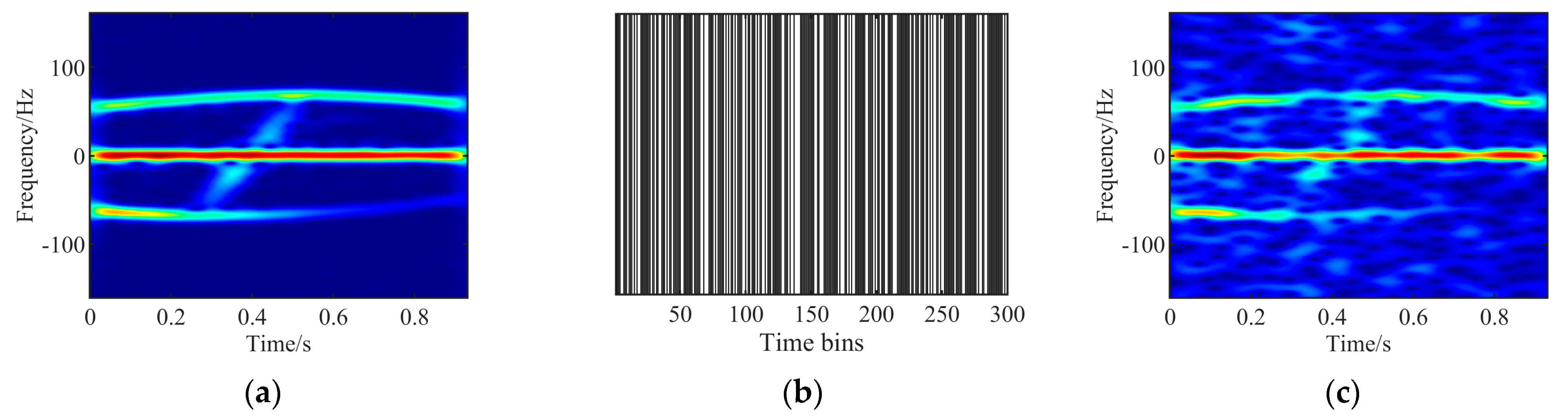
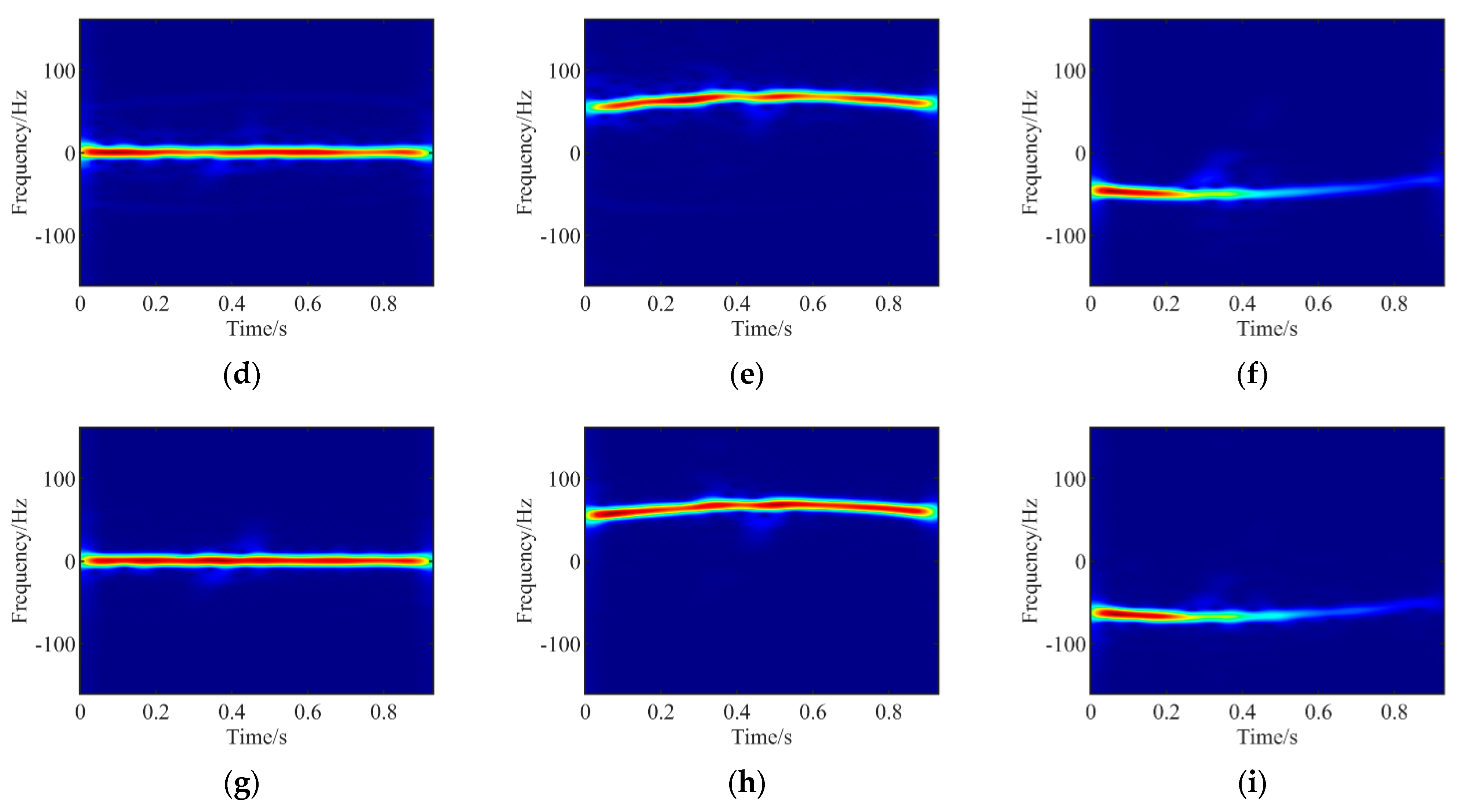
4. Experimental Results

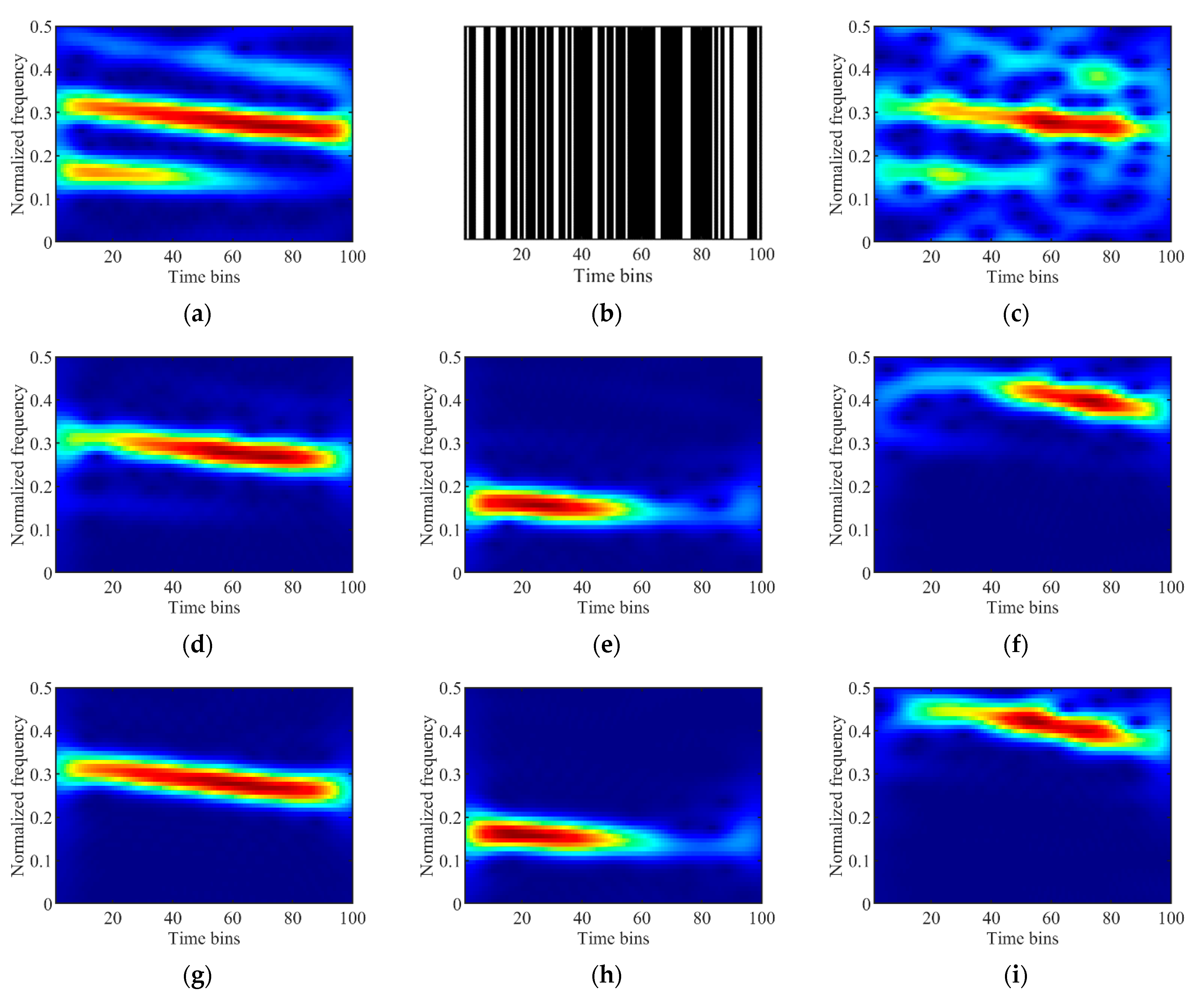
In this section, we will demonstrate the performance of the proposed method by the simulated signal, experimental data, and real-life data. The relative error $\xi$ is fixed at 0.0001 to 0.01. According to experience, the proposed method can work effectively when $\eta$ is set between 0.01 and 0.1. The step of sliding window $m_s$ is 1. The window function of STFT is the Gaussian window.

4.1. Simulated Data

As most micro-Doppler signals can be considered amplitude modulation and frequency modulation (AM-FM) signals, the proposed method is verified by multicomponent AM-FM signals. Since the IFs of returned signals of most micro-motion target scatterers are sinusoidal or linear functions, the AM-FM signal is set to consist of two SFM signal components and a linear FM signal component. The simulated AM-FM signal can be presented as

$$s(t)=s_1(t)+s_2(t)+s_2(t)+g(t)$$

(40)

with

$$\begin{array}{l}{s}_1(t)=a_1\left(t\right)\exp \left(j2\pi \left(30t+5t^2\right)\right)\\ s_2(t)=a_2\left(t\right)\exp \left(j2\pi \left(20t-\cos \left(\pi t\right)\right)\right)\\ s_3(t)=a_3\left(t\right)\exp \left(j2\pi \left(10t-\cos \left(\pi t\right)\right)\right)\end{array}$$

(41)

where $a_1(t)=1.5$, $a_2(t)=0.9(1+0.2\sin (1.8\pi t))$ and $a_3(t)=(1+0.2\cos (1.6\pi t))$. $g(t)$ represents additive Gaussian noise and SNR = 20 dB. The sampling interval is 0.01 s and 100 samples are collected. The TFR of the complete signal described by Equation (41) is shown in Figure 1a. The sampling frequency is 100 Hz. The length of the window function is 23. The collected samples are missing 40% at random. The data missing model is presented in Figure 1b where the white and black bars denote missing and available samples, respectively. The TFR of the incomplete signal is shown in Figure 1c. Because of the missing data, the TFR of the signal is defocused. Figure 1d–f shows the TFR of the three components decomposed by the IRLS-based algorithm. The computational time of the IRLS-based algorithm is 17.1 s. Figure 1g–i shows the TFR of the three components decomposed by the ADMM-based algorithm. The computational time of the ADMM-based algorithm is 28.3 s. The proposed method can effectively extract the components from missing sampling data and reconstruct the well-focused TFRs. Compared with the IRLS-based method, the signal components reconstructed by the ADMM-based method are more similar to the ideal signal without missing samples.

The relative error and regularization parameters $\lambda$ with the number of iterations are shown in Figure 2. Figure 2a,c shows the relative error curves of the IRLS-based method and the ADMM-based method with the number of iterations, respectively. Figure 2b,d shows the curves of regularization parameters $\lambda$ of the IRLS-based method and the ADMM-based method with the number of iterations, respectively. The simulation results demonstrate that as the number of iterations increases, the relative errors as well as the regularization parameters of all the micro-motion signal components show a steady downward trend and converge to the desired optimization level after several iterations.

Furthermore, the signal-to-noise ratio (SNR) is used to evaluate the performance of different methods to decompose and reconstruct the signal components, which can be calculated by

$$o=10{\log }_{10}\left(\frac{{‖s(t)‖}_2}{{‖\widehat{s}(t)-s(t)‖}_2}\right)$$

(42)

where $\widehat{s}(t)$ is the extracted component signal, $s(t)$ is the correct component signal, and a random 30% missing of the signal (see Equation (41)) is introduced to test the ACMD [16], STVMD [12], OSS [14], and the proposed method. The missing signals separated by ACMD, STVMD, and OSS are preprocessed by the TFR reconstruction method [23].

Table 1. The SNR of signal components separated by different methods.

	ADMM-Based	IRLS-Based	ACMD	OSS	STVMD
$s_1(t)$	4.64 dB	4.2 dB	3.62 dB	3.29 dB	3.37 dB
$s_2(t)$	4.58 dB	4.03 dB	3.56 dB	3.2 dB	3.38 dB
$s_3(t)$	3.21 dB	2.98 dB	2.68 dB	2.23 dB	2.31 dB

shows that the ADMM-based algorithm and the IRLS-based algorithm can extract component signals with high SNR from incomplete data. In addition, the SNR of the signal components extracted by the ADMM-based method is higher compared with the IRLS-based method.

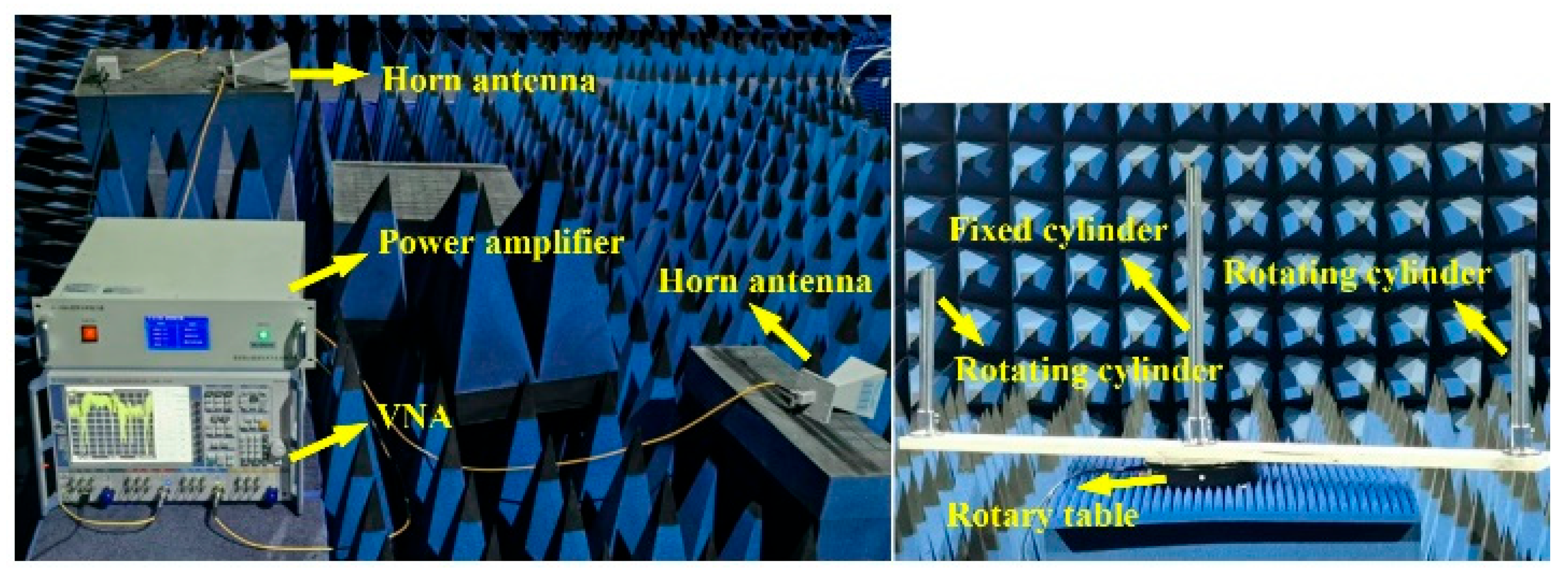
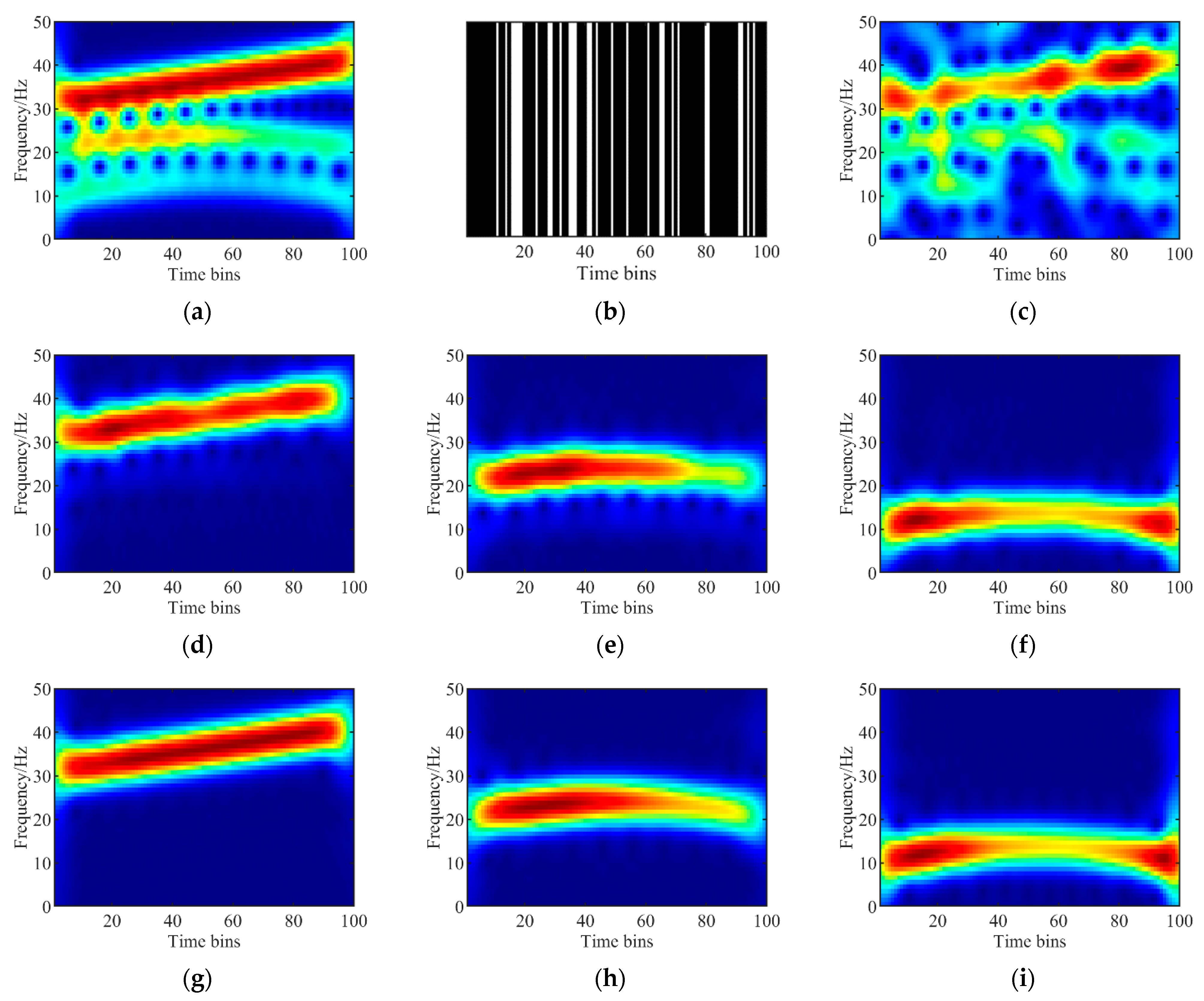
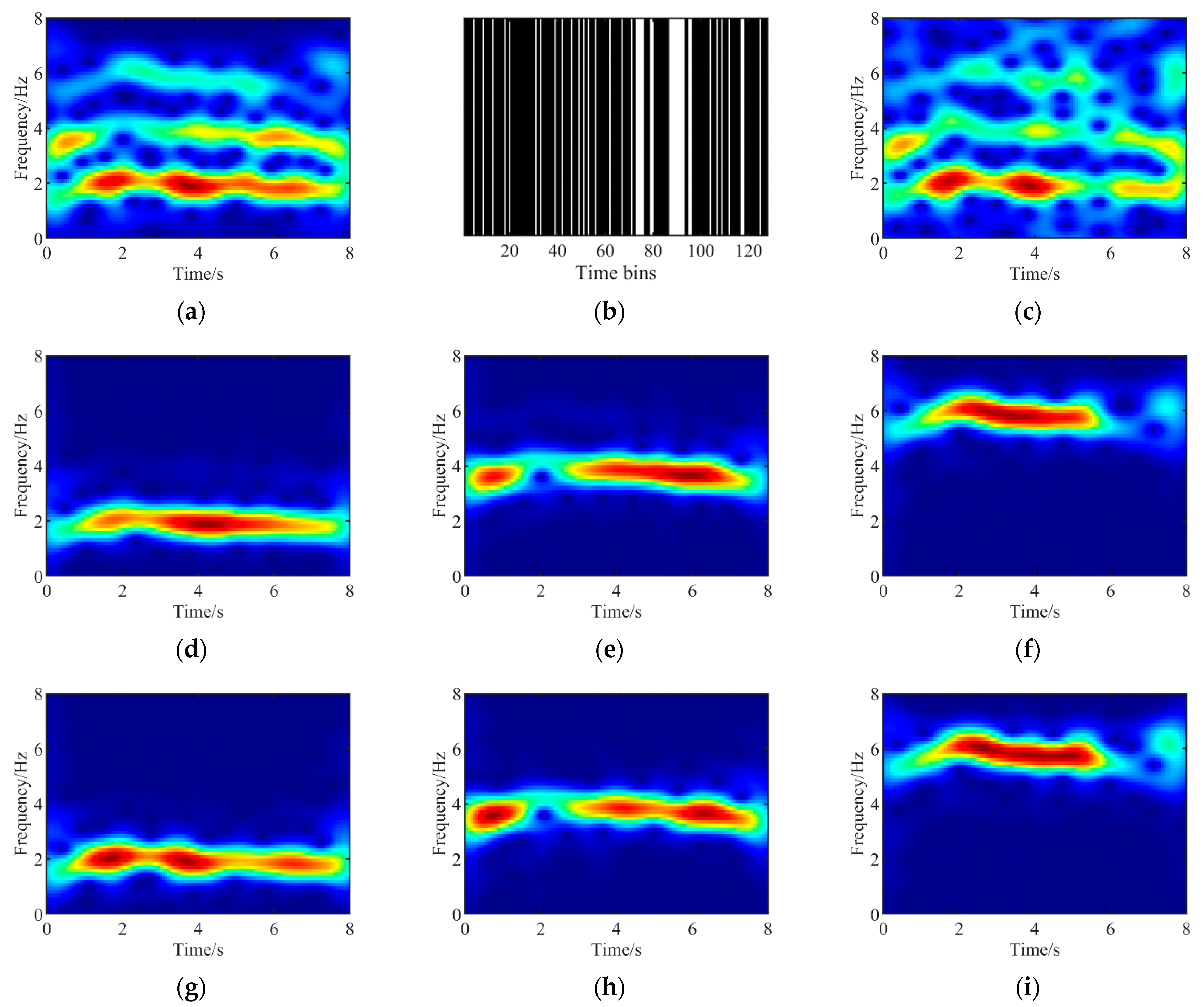
4.2. Experimental Data

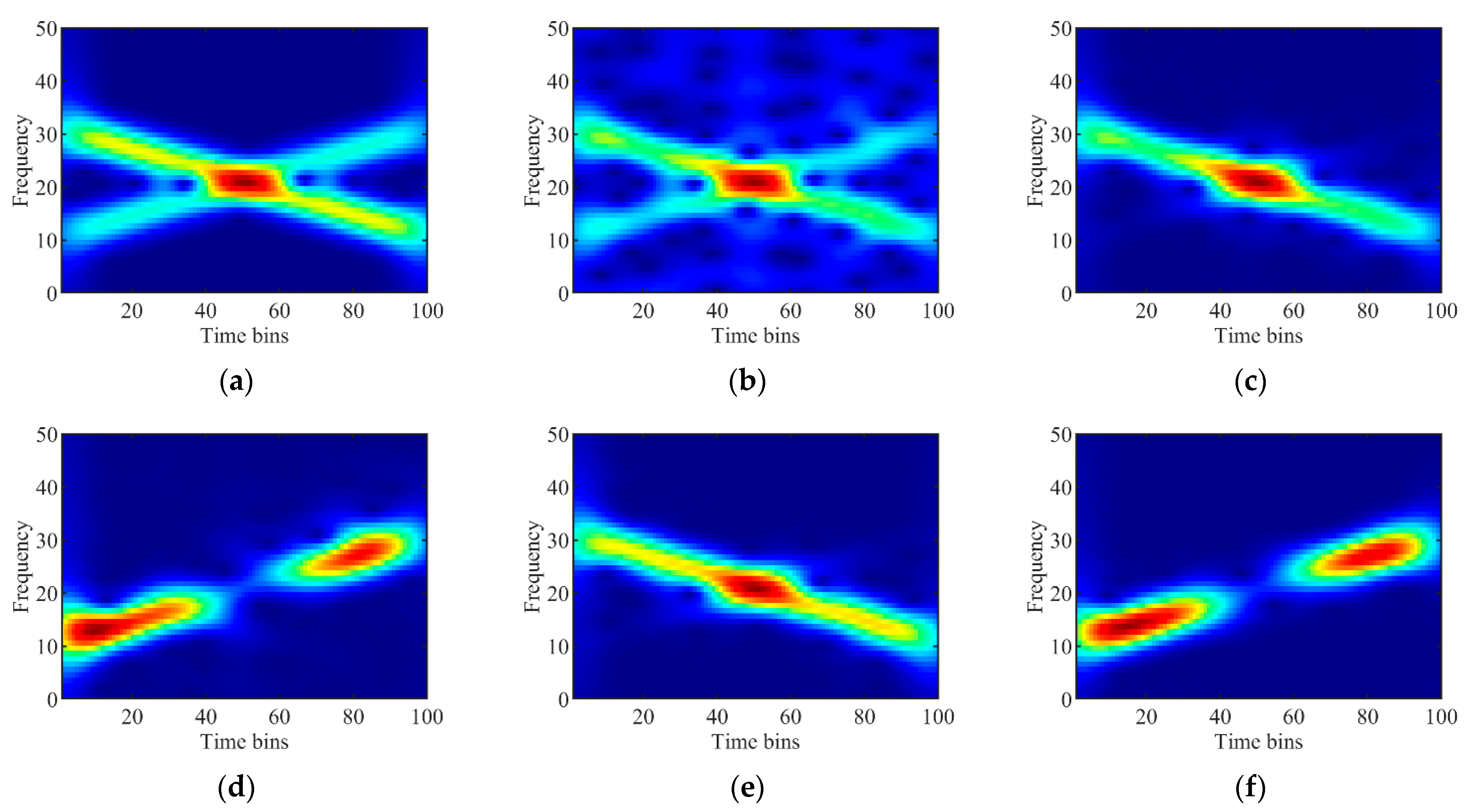
The effectiveness of the proposed method is further verified by using the returned signal from rotating targets. The experimental setup and rotating target are shown in Figure 3. The frequency of the transmit signal from the vector network analyzer (VNA) is 17 GHz. The power amplifier is used to increase the strength of the transmitted signal. The sampling interval of the returned signal is 0.0031 s. The two horn antennas are horizontally polarized. The rotating target consists of two rotating cylinders and a fixed metal cylinder. The rotating speed of the rotary table is 12 rpm.

The rotating target returned signal processed by STFT is provided in Figure 4a. The length of the window function is 53. The collected samples are missing 25% at random. The missing data model is shown in Figure 4b. The TFR with spurious peaks is shown in Figure 4c. The TFR of the three components decomposed by the IRLS-based method and the ADMM-based method are illustrated in Figure 4d–f and Figure 4g–i, respectively. The computational time of the IRLS-based algorithm and the ADMM-based method are 148.4 s and 222.6 s. As shown in Figure 4d–i, the proposed method can effectively separate and reconstruct the returned signal from the rotating target. The TF spectral entropy is introduced to compare the background noise of signals extracted by different methods [27]. In general, the lower the entropy, the smaller the background noise of TFR. The TF spectral entropy in Figure 4d–i is 3.49, 3.21, 2.75, 3.07, 3.15, and 2.68, respectively. Therefore, the ADMM-based method extracts signal components with less background noise compared with the IRLS-based method.

4.3. Real-Life Data

In this subsection, EEG data [18] and bat echolocation call signal is used to validate the proposed method.

Brain activity can be observed through electroencephalographic (EEG) signals, and extracting these EEG components is important for studying and predicting human health. In addition, similar to the returned signal of the micro-motion target, the EEG signal contains AM-FM signal components. Therefore, we used EEG signals of seizure to test the effectiveness of the proposed method. The EEG seizure data used for the analyses is selected from the EEG database [28]. The number of data sampling points is 128 and the sampling time is 8 s. The real EEG data is transformed into a complex analytic signal by the Hilbert transform for processing by the proposed method, and it can be expressed as

$$g_c\left(t\right)=g_r\left(t\right)+j\mathbf{H}\left(g_c\left(t\right)\right)$$

(43)

where $g_r\left(t\right)$ is the real EEG data, $\mathbf{H}\left(\cdot \right)$ represents the Hilbert transform, and $g_c\left(t\right)$ is the complex analytic signal. The EEG signal processed by STFT is provided in Figure 5a. The length of the window function is 33. The collected samples are missing 30% at random. The missing data model is shown in Figure 5b. The TFR of the incomplete data is shown in Figure 5c. Figure 5d–i shows the results obtained by the proposed method. The computational times of the IRLS-based algorithm and the ADMM-based method are 53.6 s and 82.3 s. As shown in Equation (42), the SNR is used to evaluate the performance of the IRLS-based algorithm and the ADMM-based algorithm, where $\widehat{s}(t)$ is the sum of the extracted component signal, and $s(t)$ is the correct signal. The SNR of the IRLS-based algorithm and the ADMM-based algorithm is 3.53 dB and 5.16 dB. Therefore, in comparison to the IRLS-based method, the ADMM-based method reconstructs more complete EEG signal components.

The sonar system of bats has many similarities with radar systems. Although bats use sound waves and radar uses electromagnetic waves to detect objects, their basic principles are the same. The proposed method is demonstrated by a bat echolocation call signal collected by Rice University, downloadable at https://dsp.rice.edu/ (accessed on 1 October 2022). The number of data sampling points is 200 and the sampling period is 7 μs. The bat echolocation call signal is also converted into the complex signal by Formula (43).

Figure 6a shows the bat echolocation call signal processed by STFT. The length of the window function is 33. The collected samples are missing at a random rate of 30%. The model of the missing data is shown in Figure 6b. The TFR of the missing data is shown in Figure 6c. Figure 6d–f shows the TFRs of the three components decomposed by the IRLS-based method, while Figure 6g–i shows the TFRs of the three components decomposed by the ADMM-based method. The computational times of the IRLS-based algorithm and the ADMM-based method are 40.3 s and 74.6 s. The results show that bat echolocation call signal components reconstructed by the ADMM-based method are smoother and more complete compared with the IRLS-based method.

5. Discussion

It should be noted that both the IRLS-based algorithm and ADMM-based algorithm extract single-component signals sequentially in a recursive framework, so the above two methods cannot thoroughly separate the energy of multicomponent signals crossing in the time-frequency domain. An example with two overlapping chirps is introduced to show this limitation.

$$s=\exp \left(j2\pi \left(10t+10t^2\right)\right)+1.5\exp \left(j2\pi \left(30t-10t^2\right)\right)$$

(44)

The analysis results for the signal in (44) by the proposed method are shown in Figure 7. The STFT of the ideal signals is shown in Figure 7a. The TFR of the incomplete signal is shown in Figure 7b. The TFR of the two components decomposed by the IRLS-based method and the ADMM-based method are illustrated in Figure 7c,d and Figure 7e,f, respectively. As shown in Figure 7c–f, the proposed method cannot effectively separate the cross-time-frequency signal. The corresponding discussion is added in the Section 6.

The echoes of the rotating components can be regarded as a sinusoidal FM signal. As shown in Figure 3, the proposed method can effectively separate the multicomponent sinusoidal FM signal. It should be pointed out that the existing work can only separate multicomponent signals that do not overlap in the time-frequency domain. Future work will focus on the application of instantaneous frequency extraction methods [17,18,19] and new algorithmic frameworks for effectively separating the energy of multicomponent signals that cross in the time-frequency domain.

6. Conclusions

In this paper, a novel method is proposed for separating multicomponent micro-Doppler signals with missing samples. The method reconstructs the incomplete data based on sparse signal representation theory and separates the reconstructed independent components according to the null space characteristics. In addition, the regularization parameters are updated adaptively during iteration. The processing results of the simulation signal, microwave darkroom data, and real-world data demonstrate that the proposed method can reconstruct the signal component from the multicomponent micro-Doppler signal with random data missing sampling, and the SNR of the signal component extracted by the ADMM-based method is higher than that of the IRLS-based algorithm. The proposed method has potential application prospects in feature extraction of micro-motion targets and automatic target recognition.

References

1. Chen, V.C.; Li, F.; Ho, S.-S.; Wechsler, H. Micro-Doppler effect in radar: Phenomenon, model, and simulation study. IEEE Trans. Aerosp. Electron. Syst. 2006, 42, 2–21. [Google Scholar] [CrossRef]
2. Hu, J.; Zhang, Q.; Luo, Y.; Chen, Y. Research progresses in radar feature extraction, imaging, and recognition of target with micro-motions. J. Radars 2018, 7, 531–547. [Google Scholar]
3. Peng, B.; Wei, X.; Deng, B.; Chen, H.; Liu, Z.; Li, X. A sinusoidal frequency modulation Fourier transform for Radar-Based vehicle vibration estimation. IEEE Trans. Instrum. Meas. 2014, 63, 2188–2199. [Google Scholar] [CrossRef]
4. He, Q.; Zhang, Q.; Luo, Y.; Sun, L. Sinusoidal frequency modulation Fourier-Bessel series for multicomponent SFM signal estimation and separation. Math Probl. Eng. 2017, 1, 5852171. [Google Scholar] [CrossRef]
5. Zhang, Q.; Yeo, T.S.; Tan, H.S.; Luo, Y. Imaging of a moving target with rotating parts based on the Hough transform. IEEE Trans. Geosci. Remote Sens. 2008, 46, 291–299. [Google Scholar] [CrossRef]
6. Wang, Z.; Wang, Y.; Xu, L. Parameter Estimation of Hybrid Linear Frequency Modulation-Sinusoidal Frequency Modulation Signal. IEEE Signal Process. Lett. 2017, 24, 1238–1241. [Google Scholar] [CrossRef]
7. Chen, X.; Guan, J.; Liu, N.; Zhou, W.; He, Y. Detection of a Low Observable Sea-Surface Target with Micro-motion via the Radon-Linear Canonical Transform. IEEE Geosci. Remote Sens. Lett. 2014, 11, 1225–1229. [Google Scholar] [CrossRef]
8. Guan, J.; Pei, J.; Huang, Y.; Chen, X.; Chen, B. Time-Range Adaptive Focusing Method Based on APC and Iterative Adaptive Radon-Fourier Transform. Remote Sens. 2022, 14, 6182. [Google Scholar] [CrossRef]
9. Dragomiretskiy, K.; Zosso, D. Variational mode decomposition. IEEE Trans. Signal Process. 2014, 62, 531–544. [Google Scholar] [CrossRef]
10. Bai, X.; Xing, M.; Zhou, F.; Lu, G.; Bao, Z. Imaging of Micro-motion Targets with Rotating Parts Based on Empirical-Mode Decomposition. IEEE Trans. Geosci. Remote Sens. 2008, 46, 3514–3523. [Google Scholar] [CrossRef]
11. Kang, W.; Zhang, Y.; Dong, X. Micro-Doppler effect removal for ISAR imaging based on bivariate variational mode decomposition. IET Radar Sonar Navig. 2018, 12, 74–81. [Google Scholar] [CrossRef]
12. Li, Y.; Xia, W.; Dong, S. Time-based multicomponent irregular FM micro-Doppler signals decomposition via STVMD. IET Radar Sonar Navig. 2020, 14, 1502–1511. [Google Scholar] [CrossRef]
13. Chen, S.; Dong, X.; Peng, Z.; Zhang, W.; Meng, G. Nonlinear chirp mode decomposition: A variational method. IEEE Trans. Signal Process. 2017, 65, 6024–6037. [Google Scholar] [CrossRef]
14. Guo, B.; Peng, S.; Hu, X.; Xu, P. Complex-valued differential operator-based method for multicomponent signal separation. Signal Process. 2017, 132, 66–76. [Google Scholar] [CrossRef]
15. Wang, H.; Li, K.M.; Zhang, Y.P.; Luo, Y.; Zhang, Q. Separation of Phase-Corrupted Multicomponent Nonlinear Chirp Signal. IEEE Geosci. Remote Sens. Lett. 2022, 19, 4025205. [Google Scholar] [CrossRef]
16. Chen, S.; Yang, Y.; Peng, Z.; Dong, X.; Zhang, W.; Meng, G. Adaptive chirp mode pursuit: Algorithm and applications. Mech. Syst. Signal Process. 2019, 116, 566–584. [Google Scholar] [CrossRef]
17. Khan, N.A.; Ali, S. A robust and efficient instantaneous frequency estimator of multicomponent signals with intersecting time-frequency signatures. Signal Process. 2020, 177, 107728. [Google Scholar] [CrossRef]
18. Chui, C.K.; Jiang, Q.T.; Li, L.; Lu, J. Time-scale-chirp rate operator for recovery of non-stationary signal components with crossover instantaneous Frequency curves. Appl. Comput. Harmon. A. 2021, 54, 323–344. [Google Scholar] [CrossRef]
19. Li, L.; Han, N.N.; Jiang, Q.T.; Chui, C. A chirplet transform-based mode retrieval method for multicomponent signals with crossover instantaneous frequencies. Digital Signal Process. 2022, 120, 103262. [Google Scholar] [CrossRef]
20. Hui, Y.; Bai, X.; Zhou, F. JTF analysis of micromotion targets based on single-window variational inference. IEEE Trans. Geosci. Remote Sens. 2021, 59, 6600–6608. [Google Scholar] [CrossRef]
21. Zhao, Y.; Feng, J.; Zhang, B.C.; Hong, W.; Wu, Y. Current progressin sparse signal processing applied to radar imaging. SCI China Technol. Sc. 2013, 56, 3049–3054. [Google Scholar] [CrossRef]
22. Li, G.; Varshney, P.K. Micro-Doppler parameter estimation via parametric sparse representation and pruned orthogonal matching pursuit. IEEE J. Sel. Topics Appl. Earth Observ. 2014, 7, 4937–4948. [Google Scholar] [CrossRef]
23. Bai, X.; Zhou, F.; Hui, Y. Obtaining JTF-signature of space-debris from incomplete and phase-corrupted data. IEEE Trans. Aerosp. Electron. Syst. 2017, 53, 1169–1180. [Google Scholar] [CrossRef]
24. Chen, X.; Yu, X.; Huang, Y.; Guan, J. Adaptive clutter suppression and detection algorithm for radar maneuvering target with high-order motions via sparse fractional ambiguity function. IEEE J. Sel. Top. Appl. Earth Observ. Remote Sens. 2020, 13, 1515–1526. [Google Scholar] [CrossRef]
25. Bai, X.; Zhou, F. Radar imaging of micromotion targets from corrupted data. IEEE Trans. Aerosp. Electron. Syst. 2016, 52, 2789–2802. [Google Scholar] [CrossRef]
26. Zhang, S.; Liu, Y.; Li, X. Micro-Doppler Effects Removed Sparse Aperture ISAR Imaging via Low-Rank and Double Sparsity Constrained ADMM and Linearized ADMM. IEEE Trans. Image Process. 2021, 30, 4678–4690. [Google Scholar] [CrossRef]
27. Yu, D.; Yang, Y.; Cheng, J. Application of time–frequency entropy method based on Hilbert–Huang transform to gear fault diagnosis. Measurement 2007, 40, 823–830. [Google Scholar] [CrossRef]
28. Boashash, B.; Khan, N.A.; Ben-Jabeur, T. Time–frequency features for pattern recognition using high-resolution TFDs: A tutorial review. Digital Signal Process. 2015, 40, 1–30. [Google Scholar] [CrossRef]
Figure 1. The analysis results of simulated multicomponent AM-FM signal. (a) TFR of the ideal signal. (b) Missing model. (c) TFR of the incomplete signal. (df) TFR of each component signal separated via IRLS-based method. (gi) TFR of each component signal separated via ADMM-based method.
Remotesensing 16 01369 g001
Figure 2. The relative error and regularization parameters with the number of iterations. (a) The relative error of IRLS-based method. (b) The regularization parameter of IRLS-based method. (c) The relative error of ADMM-based method. (d) The regularization parameter of ADMM-based method.
Remotesensing 16 01369 g002
Figure 3. Diagram of the experimental setup and rotating target.
Remotesensing 16 01369 g003
Figure 4. The analysis results of the returned signal of rotating targets. (a) TFR of the returned signal of rotating targets. (b) Missing model. (c) TFR of the incomplete data. (df) TFR of each component signal separated via IRLS-based method. (gi) TFR of each component signal separated via ADMM-based method.
Remotesensing 16 01369 g004aRemotesensing 16 01369 g004b
Figure 5. The analysis results of EEG. (a) TFR of the EEG. (b) Missing model. (c) TFR of the incomplete data. (df) TFR of each component signal separated via IRLS-based method. (gi) TFR of each component signal separated via ADMM-based method.
Remotesensing 16 01369 g005
Figure 6. The analysis results of the bat echolocation call signal. (a) TFR of the bat echolocation call signal. (b) Missing model. (c) TFR of the incomplete data. (df) TFR of each component signal separated via IRLS-based method. (gi) TFR of each component signal separated via ADMM-based method.
Remotesensing 16 01369 g006
Figure 7. Analysis results for multicomponent signals that cross in the time-frequency domain by the proposed method. (a) TFR of the ideal signal. (b) TFR of the incomplete data. (c,d) TFR of each component signal separated via IRLS-based method. (e,f) TFR of each component signal separated via ADMM-based method.
Remotesensing 16 01369 g007