Article

Early-Season Crop Classification Based on Local Window Attention Transformer with Time-Series RCM and Sentinel-1

Department of Geography and Environment, The University of Western Ontario, London, ON N6A 3K7, Canada
*
Author to whom correspondence should be addressed.
Remote Sens. 2024, 16(8), 1376; https://doi.org/10.3390/rs16081376
Submission received: 7 March 2024 / Revised: 7 April 2024 / Accepted: 11 April 2024 / Published: 13 April 2024

Abstract

:
Crop classification is indispensable for agricultural monitoring and food security, but early-season mapping has remained challenging. Synthetic aperture radar (SAR), such as RADARSAT Constellation Mission (RCM) and Sentinel-1, can meet higher requirements on the reliability of satellite data acquisition with all-weather and all-day imaging capability to supply dense observations in the early crop season. This study applied the local window attention transformer (LWAT) to time-series SAR data, including RCM and Sentinel-1, for early-season crop classification. The performance of this integration was evaluated over crop-dominated regions (corn, soybean and wheat) in southwest Ontario, Canada. Comparative analyses against several machine learning and deep learning methods revealed the superiority of the LWAT, achieving an impressive F1-score of 97.96% and a Kappa coefficient of 97.08% for the northern crop region and F1-scores of 98.07% and 97.02% for the southern crop region when leveraging time-series data from RCM and Sentinel-1, respectively. Additionally, by the incremental procedure, the evolution of accuracy determined by RCM and Sentinel-1 was analyzed, which demonstrated that RCM performed better at the beginning of the season and could achieve comparable accuracy to that achieved by utilizing both datasets. Moreover, the beginning of stem elongation of corn was identified as a crucial phenological stage to acquire acceptable crop maps in the early season. This study explores the potential of RCM to provide reliable prior information early enough to assist with in-season production forecasting and decision making.

1. Introduction

Crop monitoring is challenging on regional and national scales due to the uncertainty of meteorological conditions and local land management decisions over growing seasons [1,2,3]. In this context, crop classification based on remote sensing plays a pivotal role in providing foundational data for crop monitoring and diverse agricultural applications [4,5,6,7]. Particularly, the practice of early-season crop mapping, involving the identification of crop types during the initial stages or before harvest, has garnered significant demand from businesses involved in crop insurance, land rental, supply-chain logistics, and commodity markets [8,9]. Nonetheless, this process faces substantial research gaps due to limited satellite observations and the scarcity of current-year crop labels, which impede effective early-season crop identification.
Several early-season mapping methodologies have been developed to effectively classify crop types, even in situations where there is limited or no ground truth data available for the current year. These approaches leverage historical data to generate crop labels and prior information for early-season crop identification [9,10,11,12]. For instance, utilizing a phenological metric and meteorological data derived from MODIS NDVI time series within a predefined time frame, the study takes into account the variability in crop development across different climatic zones. The employment of a Gaussian mixture model (GMM) in one such approach enables the discrimination of winter crops from other crops with a lead time of 1.5 to 2 months before harvest [13]. Moreover, the phenology-based approach has been also used to differentiate winter wheat from other crops by comparing the seasonal changes in vegetation index across all croplands with a standard seasonal change derived from known winter wheat fields. The study successfully produced winter wheat maps for 11 provinces in China from 2016 to 2018, achieving producer’s and user’s accuracies higher than 89.30% and 90.59%, respectively [14]. Using a sample transfer strategy, the topology of different crop types in the spectral feature space was employed to generate labels, thereby supporting crop classification in a different year [15]. Nevertheless, it is important to note that these transfer strategies heavily rely on historical crop labels, making them challenging to apply in regions with limited labeled data [16]. Furthermore, these methods can only be applied in limited crop types and specific regions, while the difference in meteorological conditions and local farm management can pose significant challenges and potentially lead to the failure of these methods [17].
With the accumulation of massive satellite data, using the incremental procedure and dense remote sensing data from multi-source in the early season can achieve high-accuracy crop identification. It consists of performing a supervised classification every time a new image acquisition is available using all the previously available imagery [18]. This setup allows to analyze the evolution of the mapping quality as a function of time and therefore determine at which point in time the crop identification reaches an acceptable quality. Not only high temporal resolution optical sensor data were used but also synthetic aperture radar (SAR), which can meet higher requirements on the reliability of satellite data acquisition with its all-weather and all-day capabilities, was applied [19,20,21]. Using multiple scenes of TerraSAR-X and RADARSAT-2 data, the early-season map of corn and soybean in eastern Canada was identified using a decision tree method. It found that corn could be accurately identified by the end of June, a mere six weeks after nominal planting. However, soybeans required additional acquisitions of TerraSAR-X and RADARSAT-2 [22]. The incremental classification scheme can not only monitor the accuracy evolution but also determine the stopping dates to make sure of two objectives of earliness and accuracy [23]. The development of SAR constellation systems in recent years, such as Sentinel-1A/B and RADARSAT Constellation Mission (RCM), increased the opportunity to build temporally rich datasets in the early weeks of crop growth [24,25]. RCM, as a novel SAR satellite constellation provided by the Canadian Space Agency (CSA), offers multiple polarization modes including single, dual, full, and compact polarization. This diversity enhances its utility for various Earth observation applications. Conversely, Sentinel-1, operated by the European Space Agency (ESA), stands out as the most utilized SAR data source due to its global coverage, accessibility, and no-cost access. Both RCM and Sentinel-1 operate in the C-band radar frequency and offer frequent revisit observation intervals, typically less than two weeks. These characteristics make them well-suited for precision agricultural applications, particularly in crop monitoring. To our best knowledge, there is no study that has examined the potential of RCM for early-season crop mapping.
To effectively mine the key information in time-series satellite images, deep learning methods have been widely applied in early-season crop mapping in recent years. In order to determine the earliness of prediction of crop cover maps, an End-to-End Learned Early Classification of Time Series (ELECTS) model was proposed, which can estimate a classification score and a probability of whether sufficient data have been observed to come to an early and still accurate decision [23]. Starting from yearly static reference and characterizing the different crop presence temporally by performing a phenological analysis of historical time series, the short-term ground truth maps, which specifically for Sentinel-2 feature a 5-day reference, were generated. The study presented using 3D convolution neural network (CNNs) to generate a crop map of the current season at a specific point in time as well as all intermediate maps during the season able to describe in near real time the evolution of crop presence [11]. However, the main concern of deep CNNs is that they demand more training data to fit rapidly increasing model parameters, leading to a high demand of computational resources [26,27]. The architectures with more layers and parameters such as VGG-16, AlexNet, and ResNet require more training data to fit the model parameters, which are not easy to be used for the small training data applications [28,29]. Although the transfer learning scheme based on deep learning approaches helps to gain crop mapping results in transfer sites, abundant historical labels of crop type are required [30]. Recently, attention mechanisms have been successfully applied in vision applications, e.g., weed detection and the crop classification of high-resolution UAV images [31]. However, the utilization of the attention mechanism is constrained by the high computational cost, given that the number of pixels in a satellite image far exceeds the number of units of words in natural language processing. Jamali et al. [26] proposed a local window attention transformer (LWAT) for polarimetric SAR image classification, which can balance the size and receptive fields and computational cost. Consequently, this paper aims to address three research questions: (1) Can the LWAT be applied to achieve early-season crop classification using multi-source time-series SAR data? (2) Does Sentinel-1 with dual polarimetry or RCM with compact polarimetry outperform the other for early-season crop mapping? (3) What is the optimal date and phenological stages to obtain an acceptable crop map while ensuring timeliness?
To address the research questions, this study aims to explore the potential of time-series Sentinel-1 and RCM data for early-season crop classification. The LWAT is selected to apply to this application. Unlike self-attention, LWAT enhances feature representation within local contexts while significantly reducing annotation costs and hardware requirements. The method was tested using Sentinel-1 and RCM, covering the period from 29 May to 12 July 2022, over two crop-dominated regions (corn, soybean, and wheat) in southwest Ontario, Canada. The study quantitatively evaluated the performance of early-season crop mapping using Sentinel-1 and RCM, providing an analysis of the accuracy evolution of dominant crops. Finally, the optimal date and their corresponding phenological stage were identified to achieve both earliness and accuracy.
The main contributions of this paper are as follows.
(i)
The integration of the LWAT with time-series SAR data for early-season crop mapping.
(ii)
A comparative analysis of the performance of Sentinel-1 and RCM for early-season crop classification.
(iii)
Determination of the optimal date and phenological stage to achieve both earliness and accuracy for early-season crop mapping.

2. Study Area and Data
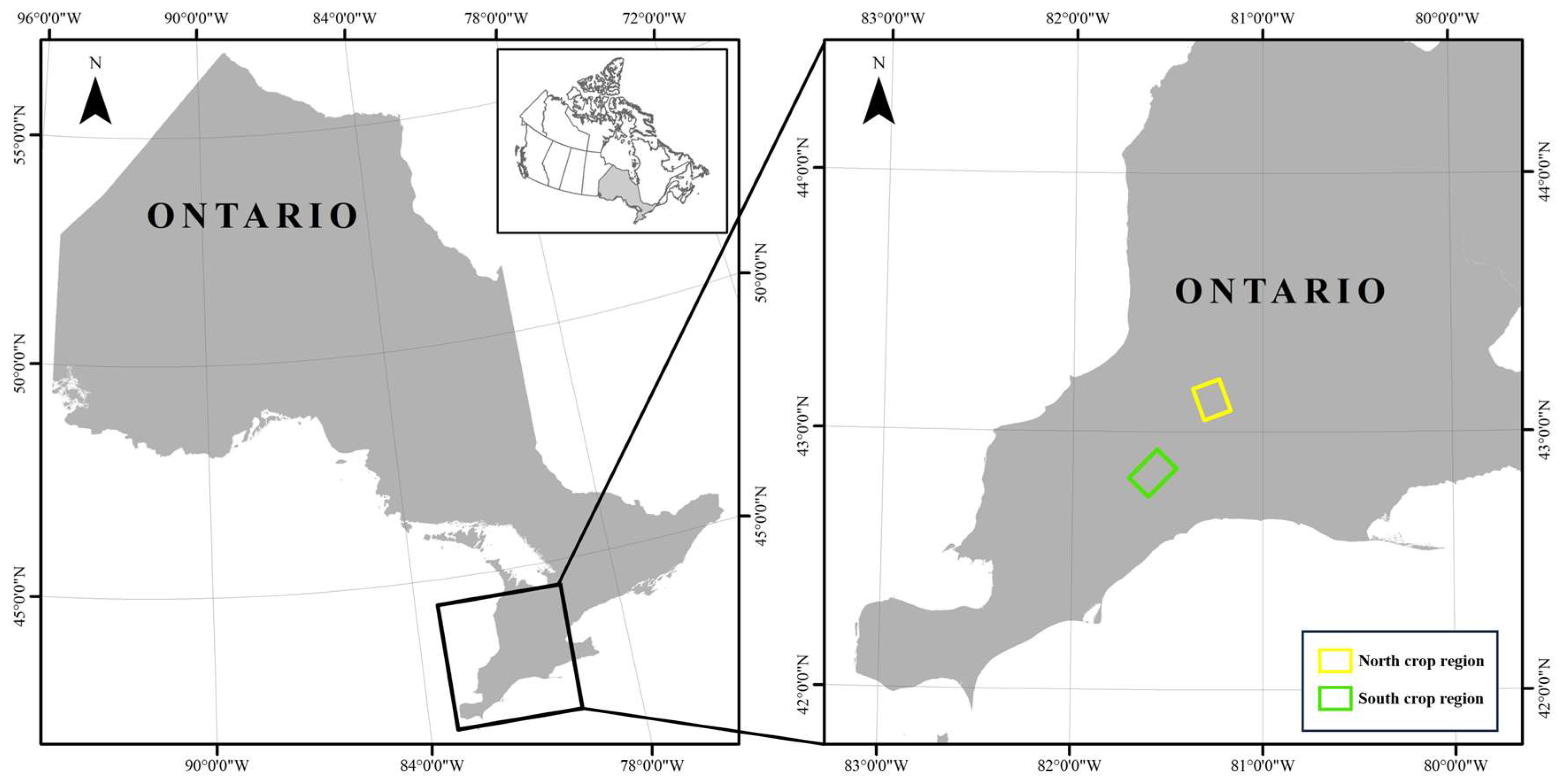
2.1. Study Area

Two crop regions near London City, southwest Ontario, Canada, were selected for this study, as shown in Figure 1. The northern crop region (yellow rectangle) covers an area of approximately 170 km2, while the southern crop region (green rectangle) spans around 200 km2. The major crops in this region include corn, soybean, and winter wheat. Here, the early season is defined as the end of May to early July within six to eight weeks after the spring seeding of corn and soybean. In contrast, winter wheat in this study site was planted in October of the previous year and harvested in July of the following year [7,32]. Thus, the early season is only for corn and soybean in this study. Notably, in addition to the fields planted with the above crops, some fields might be followed by growers and planted with cover crops, such as alfalfa and forage [33]. These cover plants were merged into the grass category, which needs to be discriminated from major crops. Other ground cover types are woodland, build-up, and water.

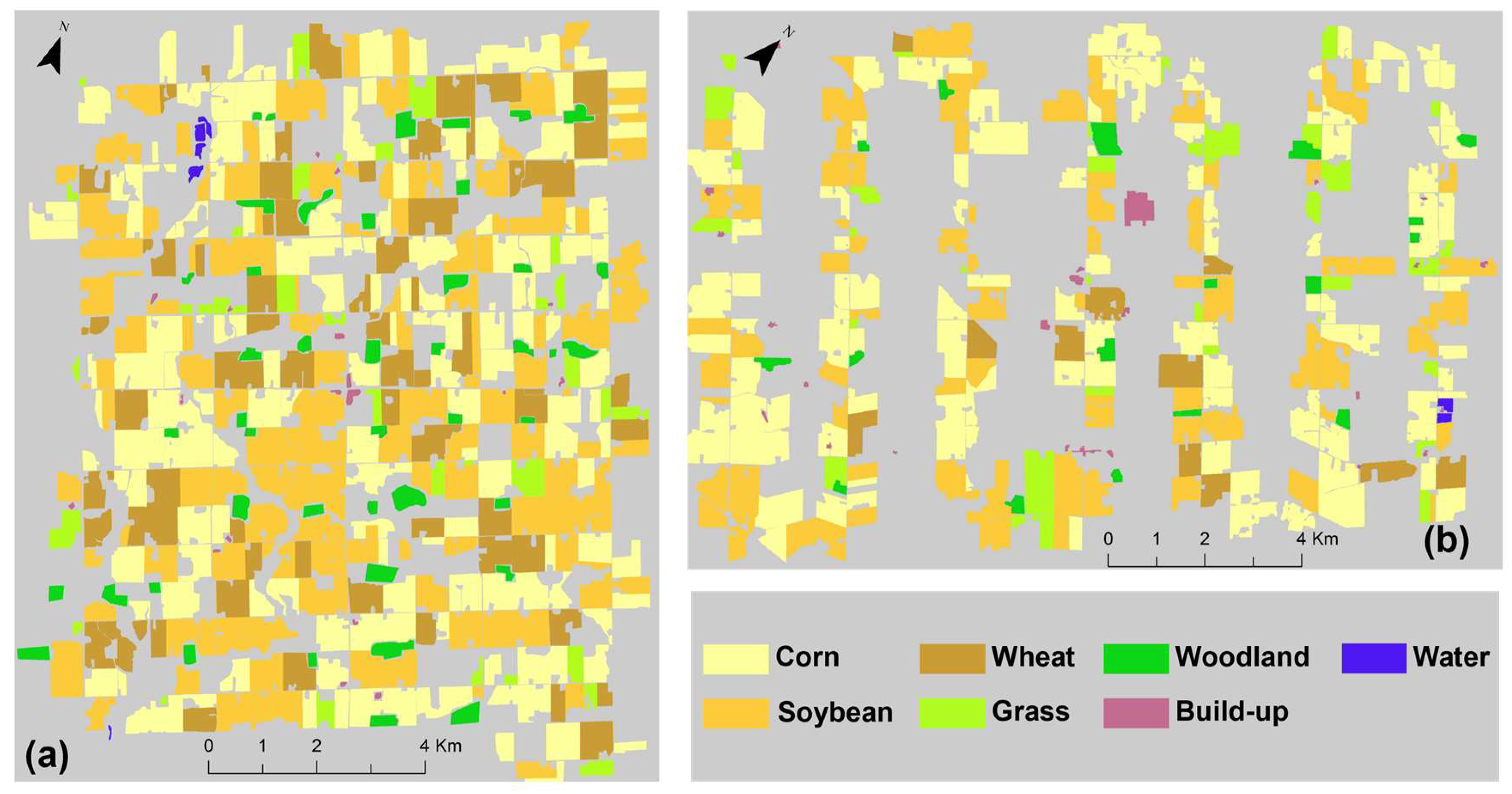
2.2. Ground Truth Data

The ground truth data for crop classification are from our annual crop inventory. The ground survey was taken in the middle of July 2022. In this season, winter wheat was matured and corn and soybean were easily identified. After recording locations and crop types, manual digitization was carried out using ArcMap software based on high-resolution satellite images like Planet Scope and Sentinel-2 to generate the crop-type polygons (Figure 2). Finally, these polygons were converted into a ground truth image and randomly divided into five datasets for training and validation at the pixel scale. This division served to obtain the mean and standard deviation of accuracy by conducting experiments five times. In total, 70% of the data were used for training, while the remaining 30% served as validation data. For our study, patches with a local window size of 12 × 12 were utilized for generating training and validation sets. In the case of the northern crop region, a total of 378,647 patches were employed for training with an additional 882,915 patches designated for validation. In the southern crop region, the training dataset comprised 115,478 patches, and 269,252 patches were used for validation purposes. Furthermore, phenology information for corn and soybean was collected using the BBCH values [34]. The general phenology stages of corn are from leaf development to stem elongation, while the stages of soybean are from leaf development to flowering. Some field photos and their corresponding phenological stages are shown in Figure 3.

2.3. Satellite Data

In this study, satellite data from both Sentinel-1 and RCM were selected. Four scenes of dual-polarization (VH and VV) Sentinel-1 data with the Interferometric Width (IW) mode are provided by the ESA, as shown in Table 1. Although the ESA announced the revisit time of using two satellites is 6 days, only Sentinel-1A was working in our study site, and Sentinel-1B’s mission ended on 3 August 2022 due to an anomaly related to the instrument electronics power [35]. Our study area is located in an overlap of two orbits (orbit number 77 with an incidence angle of 31.5° and orbit number 150 with an incidence angle of 41.5°) of Sentinel-1, causing the data access frequency to be less than 12 days [7]. Six scenes of RCM data were provided by the CSA, spanning from 29 May to 12 July 2022. Unlike the commonly used linear polarization modes, such as HH and VV polarization, RCM utilizes compact polarimetry, transmitting right circular radar signals and receiving horizontal (RCH) and vertical (RCV) directions [36]. Compact polarimetry offers richer information about SAR scattering compared to single and dual-polarizations and comes with swath widths significantly larger than fully polarimetric modes [37]. RCM, with its constellation of three identical satellites, has the capability to provide 4-day repeats and more frequent revisits of any given target. In our study area, the typical revisit time for RCM data is around 8 days, allowing us to capture changes and variations of crops at a relatively high frequency. This temporal resolution ensures that earth observation does not miss any phenological stages of crop growth, thereby enhancing the identification of crop types using time-series SAR data. The spatial resolution of the RCM data used in our study is 5 m, providing fine details for crop identification. This 5 m spatial resolution allows for a clear delineation of field boundaries, providing more accuracy than SAR images with coarser spatial resolutions. The combination of higher spatial and temporal resolutions enables the effective monitoring of early-season crop types. For the northern crop region, both Sentinel-1 and RCM covered the entire area, while only Sentinl-1 visited the southern crop region.

3. Method

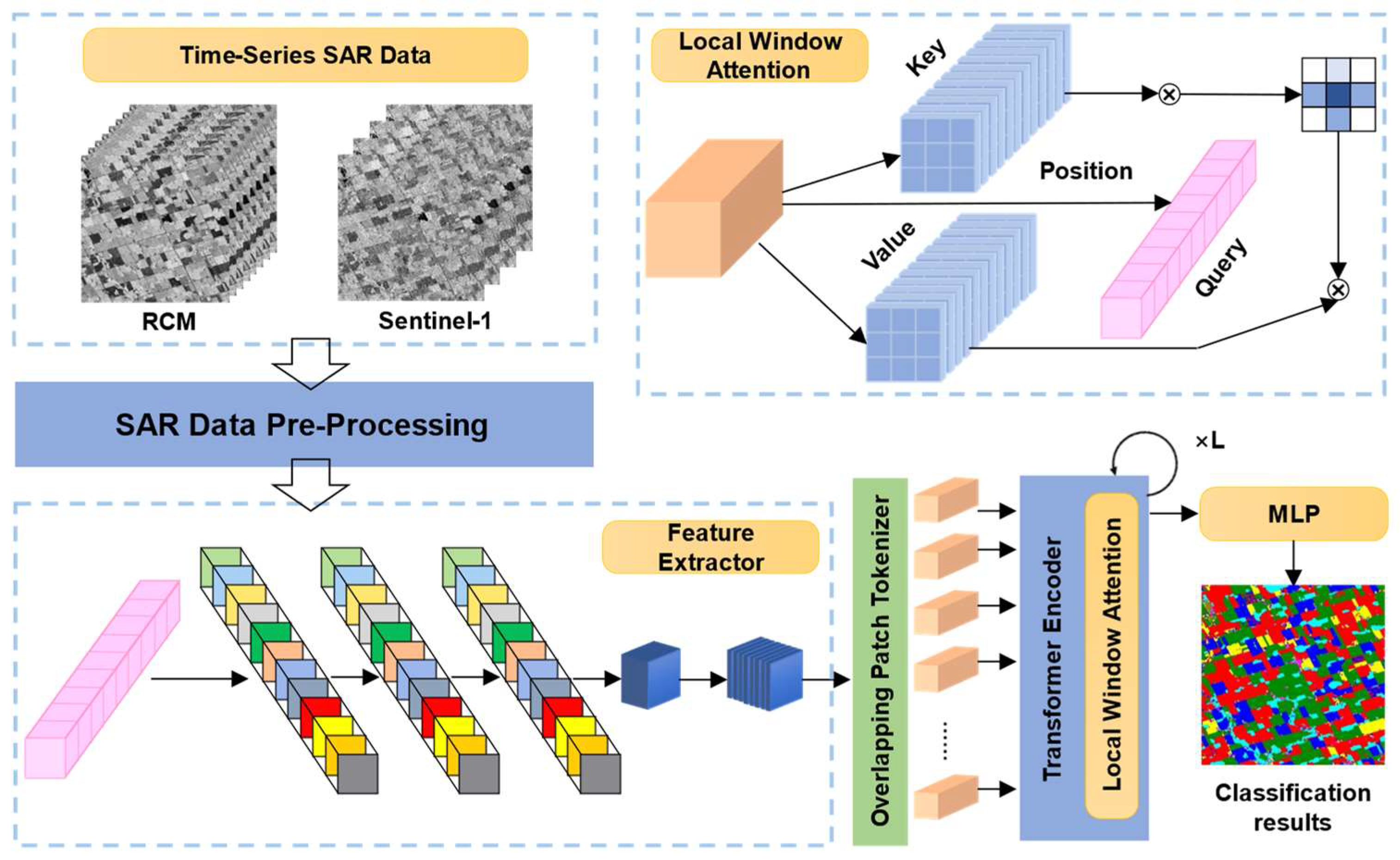
3.1. SAR Data Pre-Processing

The pre-processing steps applied to the Sentinel-1 and RCM data consist of radiometric calibration, multilook processing, speckle filtering, co-registration, and terrain correction using the SNAP software. The time-series SAR data were firstly processed with the radiometric calibration, aiming to provide imagery where digital values directly relate to the radar backscatter of the scene. After calibration, the digital values were converted to sigma nought values using the appropriate calibration look-up tables. SAR images typically exhibit inherent speckles, which can hinder image interpretation. To mitigate the influence of speckle noise, the multilook processing was applied, which not only reduces speckle but also allows us to generate an application product with a nominal image pixel size [22]. In multilook processing, a single-look SAR image is averaged over a small sliding window in both the azimuth and range directions in the space domain. This averaging process helps to smooth out speckle noise while preserving important image features. For RCM, 3 looks in the range and 4 looks in the azimuth direction were used, while for Sentinel-1, 4 looks in the range and 1 look in the azimuth direction were used. In addition to multilook processing, a speckle filtering technique using a 3 × 3 boxcar filter was applied for each RCM and Sentinel-1 scene to further reduce speckle appearance. To create a coherent time series of SAR images, co-registration was performed by selecting one image as the master reference, and the other images were resampled to match the geographical raster of the reference product. When SAR data are acquired from a satellite, the sensor is not always directly overhead (nadir), resulting in oblique viewing angles. This oblique viewing angle, combined with the uneven terrain elevation, causes geometric distortions in the acquired imagery. Terrain corrections are intended to compensate for these distortions so that the geometric representation of the image will be as close as possible to the real world. Lastly, the rectified image after terrain correction is output in the WGS84 geographic coordinate system. Additionally, the spatial resolution of the raster grid for both Sentinel-1 and RCM data was standardized to 10 m. This adjustment ensured that the images from both sensors had uniform dimensions and could be seamlessly compared and integrated during subsequent analysis.

3.2. Local Window Attention Transformer (LWAT)

This study introduces a practical framework for early-season crop mapping by integrating the LWAT with time-series RCM and Sentinel-1 data. The LWAT, originally proposed in [26], comprises two integral components: a feature extractor and a local window attention (LWA) module, which is depicted in Figure 4, offering a comprehensive solution for effectively classifying crops in the early crop growing season.
The feature extractor within the LWAT framework is intricately designed with a hierarchical architecture, harnessing the capabilities of both 3D and 2D CNNs. Originally intended to extract valuable insights from higher-dimensional polarimetric features, the 3D CNNs are employed in this study to process the time-series stack of backscattering coefficients obtained from RCM and Sentinel-1. Effectively capturing spatial and temporal features inherent in SAR data over crop regions, these 3D CNNs play a crucial role in feature extraction. Through a sequence of three consecutive 3D CNN layers, the spatial information of SAR data is thoroughly explored. Subsequently, a 2D CNN is introduced to refine prominent spatial features, thereby optimizing computational efficiency without compromising accuracy. Noteworthy is the specifications of kernel sizes for the 3D CNNs (16, 32, 64) and the 2D CNN (12), which are tailored to the characteristics of the data. This feature extractor, as corroborated by prior research [26], comprises three 3D convolutional layers followed by a 2D convolutional layer, underscoring its efficacy in extracting pertinent features essential for crop classification tasks. The resulting high-dimensional features are then fed into the LWAT module to obtain a more representative feature representation.
The LWAT module plays a pivotal role in enhancing the classification process by incorporating a local attention mechanism. Unlike conventional CNN architectures, which utilize local receptive fields, typically a K × K grid, where each output pixel depends on a small neighborhood of input pixels, the LWAT module adopts a self-attention mechanism that considers all input pixels when computing the new value of a pixel. However, employing a too large receptive field may result in high computational costs.
The LWA mechanism addresses this challenge by allowing the localization of each query’s receptive field within a defined window, thereby facilitating the efficient management of receptive fields without imposing additional computational burdens. For pixels within a specific window, the input sequence X is denoted as x 1 , x 2 , , x n to represent the original feature values. The transformer then converts X into three vectors, including key (K), query (Q) and value (V), corresponding to different weight vectors (denoted as Wk, Wq, and Wv), with d k representing the dimensionality of key values. The attention map is generated using the following equation [38].
Attention Q , K , V = softmax Q K T + R d k V
where R represents the relative position bias, aiding in capturing positional information, particularly in sequences. These biases enable tokens to attend more to nearby tokens and less to distant ones. In contrast to the self-attention scheme, LWA restricts the receptive fields of each token to the neighbor region [26]. This compromise between the size of the receptive field and computational costs enables LWA to effectively capture intricate spatial patterns from feature sequences while ensuring acceptable computational expenses. Additionally, when the size of the local window exceeds the receptive field, LWA behaves similarly to the self-attention scheme.

3.3. Comparison Methods

In this study, to underscore the performance of the LWAT, several traditional machine learning methods as well as deep learning models are selected for comparison purposes. These include the support vector machine (SVM), random forest (RF), VGG-16, AlexNet, 2DCNNs, ResNet-50, and Swin Transformer (ST).
Among the machine learning methods, SVM stands out as a well-established supervised learning algorithm renowned for its versatility in handling both linear and non-linear classification tasks. By optimizing a hyperplane to separate classes within the feature space, SVM demonstrates robust performance across various domains [1]. RF, an ensemble learning technique, exhibits resilience to overfitting while effectively capturing intricate relationships within high-dimensional data through the aggregation of decision trees [7,8]. Deep learning models such as VGG-16 and AlexNet have revolutionized image classification tasks with their hierarchical architectures and powerful feature extraction capabilities [29]. VGG-16, characterized by its simplicity and depth, employs 3 × 3 convolutional filters to extract features hierarchically, while AlexNet pioneered techniques such as ReLU activation functions and dropout regularization. Additionally, 2DCNNs represent a broad category of deep convolutional neural networks tailored for image processing tasks, leveraging multiple layers of convolutions and pooling for feature extraction [23]. The ResNet-50 architecture introduces the concept of residual connections to alleviate the vanishing gradient problem in deep networks, thereby facilitating the training of deeper models. With 50 layers, ResNet-50 achieves remarkable performance in image classification, object detection, and related computer vision tasks [39]. Finally, the ST model offers a novel fusion of transformer and convolutional architectures, harnessing hierarchical designs to effectively capture both local and global information within images [31].

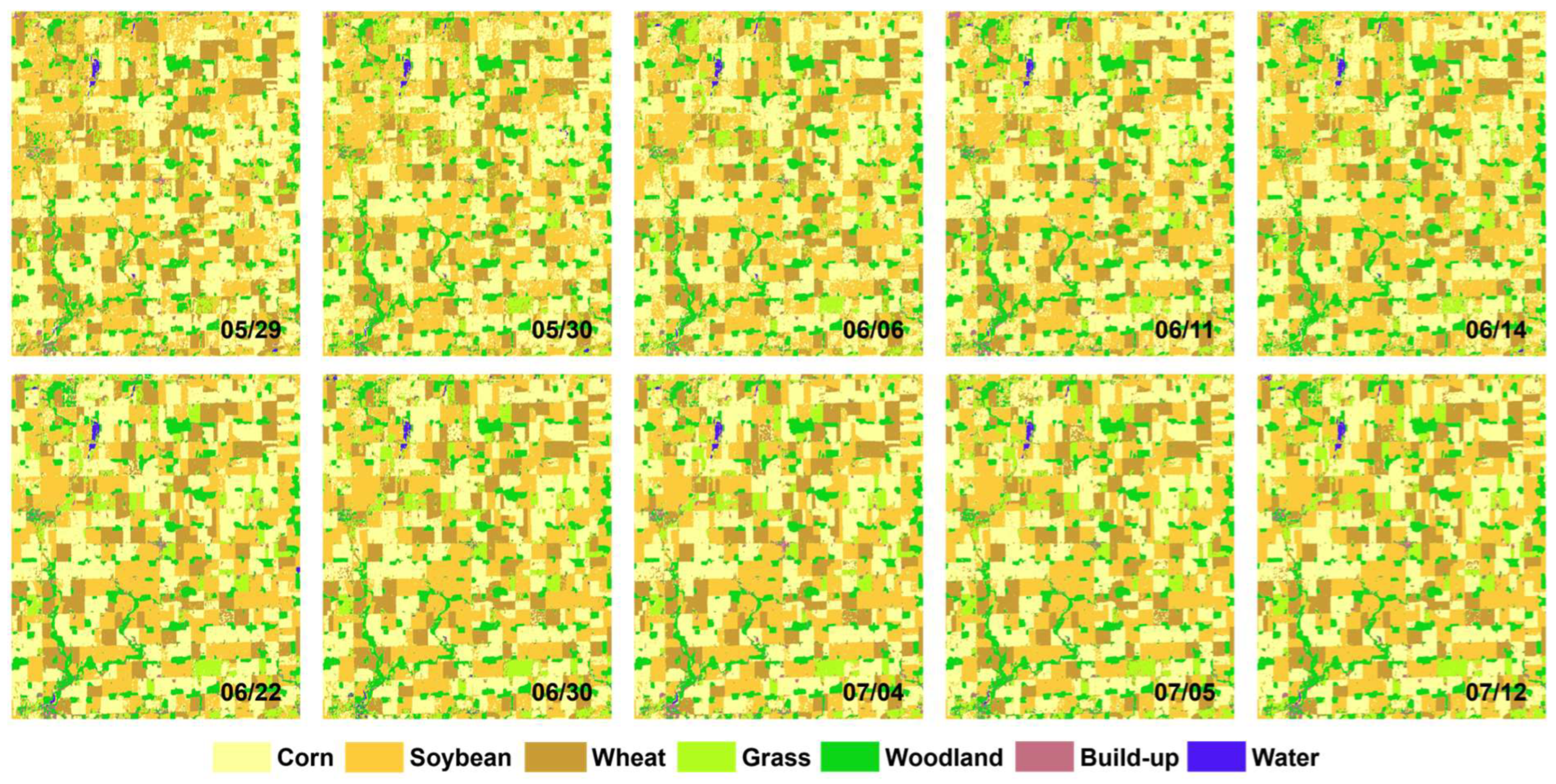
3.4. Incremental Classification

In order to monitor the accuracy evolution and determine the optimal dates for early-season crop mapping, the incremental classification scheme was applied. It consists of performing a supervised classification every time a new image acquisition is available using all the previously available imagery [18]. In the case of this study, every new SAR acquisition, either the Sentinel-1 or RCM, triggers a new model training and prediction of crop maps. Moreover, the incremental procedure was applied to not only the Sentinel-1 and RCM data individually but also to their combined dataset. This approach aims to compare the performance of early-season crop mapping when using different datasets as inputs.
The validation protocol uses 70% of the reference data for training and the remaining 30% for validation. The random split between the 2 sets is performed at the pixel level, which ensures that a pixel used for the training step is not used for the validation. Two metrics, including F1-score and Kappa coefficient, were selected to evaluate the classification results quantitatively.
The LWAT approach introduced in the previous section was used for supervised classification compared with other machine learning and deep learning methods. The Adam optimizer with a learning rate of 0.001 and a dropout rate of 40% were applied to improve generalization. To efficiently train the models, a batch size of 256 was set. Leveraging the computational power of a GeForce RTX 3090Ti, the training process took a few minutes to tens of minutes, depending on the volume of the SAR time series.

4. Experiment and Results

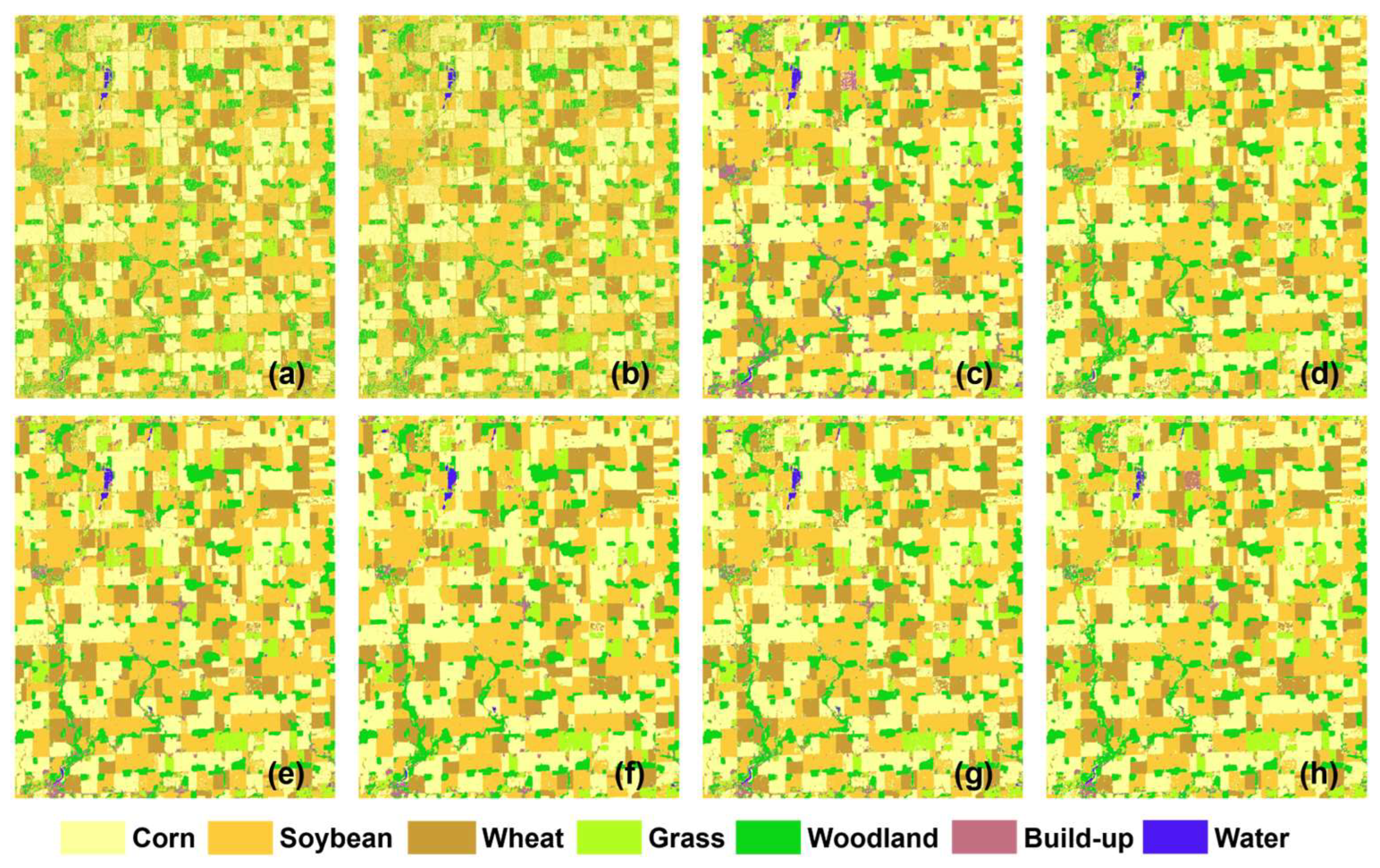
4.1. Crop Classification Using the LWAT with RCM Data

In this part, the LWAT will be compared with several traditional machine learning methods as well as deep learning models, including the SVM, RF, VGG-16, AlexNet, 2DCNNs, ResNet-50, and ST. The objective of this comparison is to demonstrate the effectiveness of LWAT in early-season crop mapping. The input data are six scenes of RCM time series captured between 29 May and 12 July 2022, which covers the northern crop area. In order to reduce the discrepancy of feature extraction steps, the backscatter of two polarization channels, i.e., RCH and RCV, serves as the input data. This choice is based on the underlying belief that the feature extractor within the LWAT model possesses the capability to extract high-dimensional features, thereby negating the need for manually designed features as input. Thus, the input data consist of a total of 12 bands with two bands corresponding to each phase of the image.
Figure 5 illustrates the classification maps using eight selected methods. Overall, the classification maps generated by two machine learning approaches, including SVM and RF, exhibit a higher presence of speckle noise compared to deep learning approaches. This discrepancy can be attributed to that deep learning methods can utilize neighboring pixels by CNN architectures to suppress speckle noise for both training and prediction, significantly reducing the occurrence of salt noise in the classification outcomes. The inherent speckle noise present in SAR images results in misclassifications between corn and soybean as well as grassland. By contrast, the deep learning methods produce smoother classification results due to their proficiency in extracting high-dimensional features from surrounding pixels, consequently mitigating the influence of speckle noise on the final outcomes.
Table 2 presents the quantitative evaluation of classification results, with the F1-score provided for each category, as well as the F1-score and Kappa coefficients for the overall assessment. The number highlighted in bold indicates the highest accuracy achieved. In Table 2, deep learning methods consistently outperformed SVM and RF in terms of accuracy across most crop categories. For the three most dominant crop types, the average F1-score of the deep learning method exceeds 95%. Notably, while LWAT did not exhibit the highest accuracy in water, woodland, and grassland categories, it achieved an impressive F1-score of 97.96% and a Kappa of 97.08%, outperforming other deep learning methods in major crops. The ResNet-50 consistently maintained accuracy above 96%, except for the build-up category, reaching notable accuracy levels of 96.65% for grass and 98.88% for water. Despite its high performance, ResNet-50 displayed a relatively higher standard deviation compared to VGG-16, which is another competitive classifier with an F1-score of 97.68% and a Kappa of 96.67%. Meanwhile, 2DCNN excelled in the woodland category, attaining an F1-score of 97.42% and a Kappa of 96.29%, with the smallest standard deviation among all deep learning methods, indicating its stability. On the other hand, AlexNet and ST methods, facing challenges in the build-up region, demonstrated lower performance than other deep learning methods. In summary, the LWAT method showcased superior performance compared to traditional machine learning and other deep learning classifiers, especially in terms of accuracy for the majority of land-cover types, particularly for the three dominant crop categories.

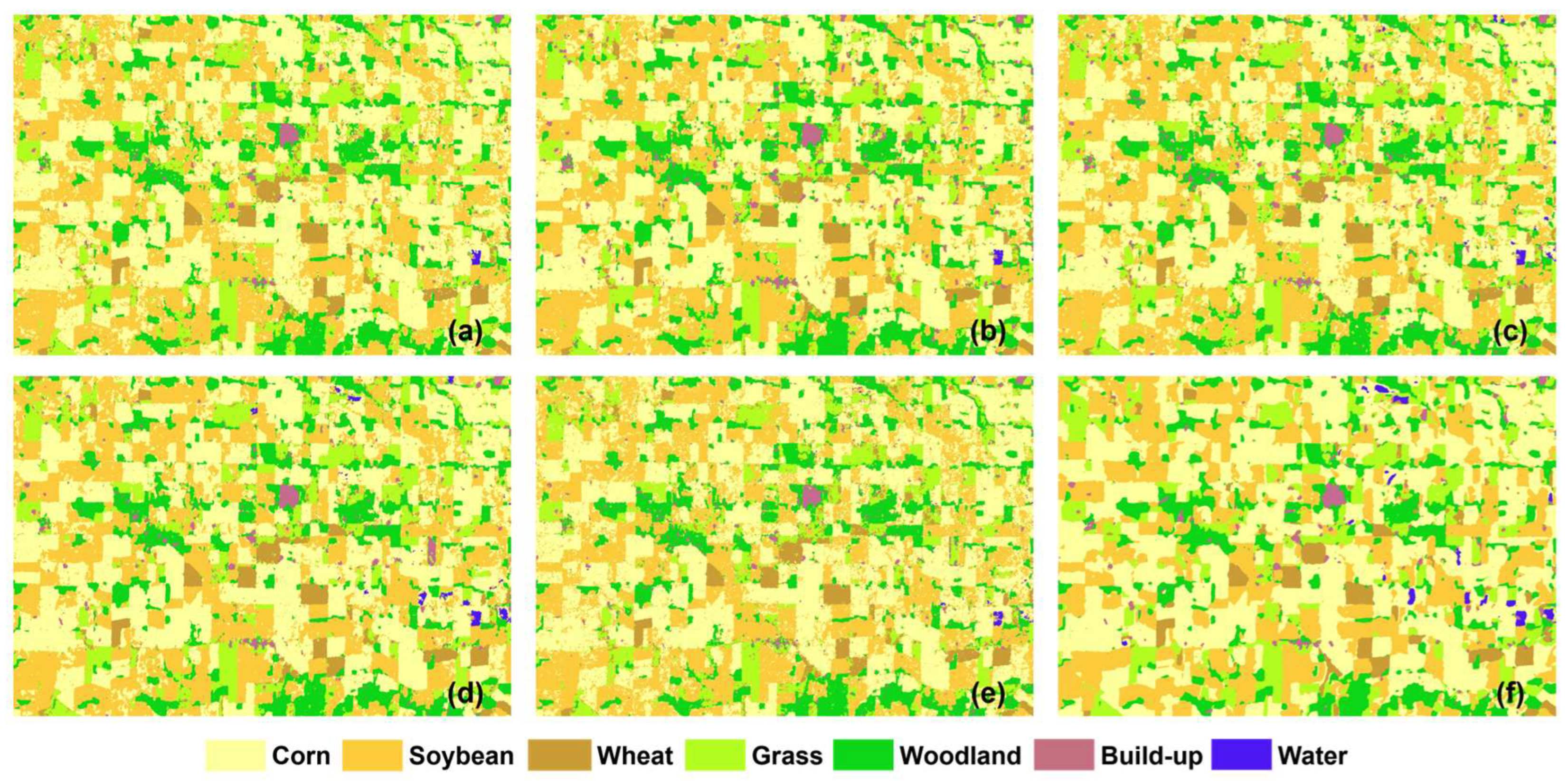
4.2. Crop Classification Using the LWAT with Sentinel-1 Data

In this section, the LWAT is compared with other deep learning approaches using Sentinel-1 time-series data to demonstrate its capabilities across different datasets. The input data consist of four scenes of Sentinel-1 data captured between 30 May and 5 July 2022, covering the southern crop region as depicted in Figure 1. In contrast to RCM’s CP bands, the backscattering coefficients of VH and VV polarization channels were utilized. Thus, the input data comprise a total of eight bands with two bands corresponding to each phase of the image.
Figure 6 illustrates crop classification maps for the southern crop region generated by various deep learning models. Overall, when compared to classification maps derived from RCM data, Sentinel-1 results exhibit more speckles, particularly for the soybean class. Among the six methods, VGG-16, 2DCNN, and ST show less smoothness compared to the results obtained by the remaining three methods, impacting the overall effectiveness of crop identification. Notably, AlexNet, which did not perform well with RCM data, exhibits improved performance with Sentinel-1 data. In contrast, LWAT demonstrates advantages in spatial coherence and the smoothness of the classification map.
Table 3 provides a quantitative evaluation of the six methods, aligning with the visual results in Figure 6. The table includes the F1-score for each category as well as the F1-score and Kappa coefficients for the overall assessment. The number highlighted in bold indicates the highest accuracy achieved. The ST method achieved an F1-score of 93.58% and a Kappa of 90.20%, which were influenced by lower accuracy in corn and soybean classes. VGG-16 and 2DCNN attained Kappa coefficients of 94.62% and 95.29%, respectively, with accuracy exceeding 96% for the three dominant crops. AlexNet demonstrated a performance comparable to ResNet-50 in terms of average accuracy but with a lower level of standard deviation. LWAT outperformed all other methods, achieving around 98% accuracy for corn, soybean, and wheat. It is the top-performing method among the six, boasting an F1-score of 98.07% and a Kappa of 97.02%. The classification results derived from both RCM and Sentinel-1 data showcase the excellent performance and adaptability of the LWAT method across diverse SAR datasets.

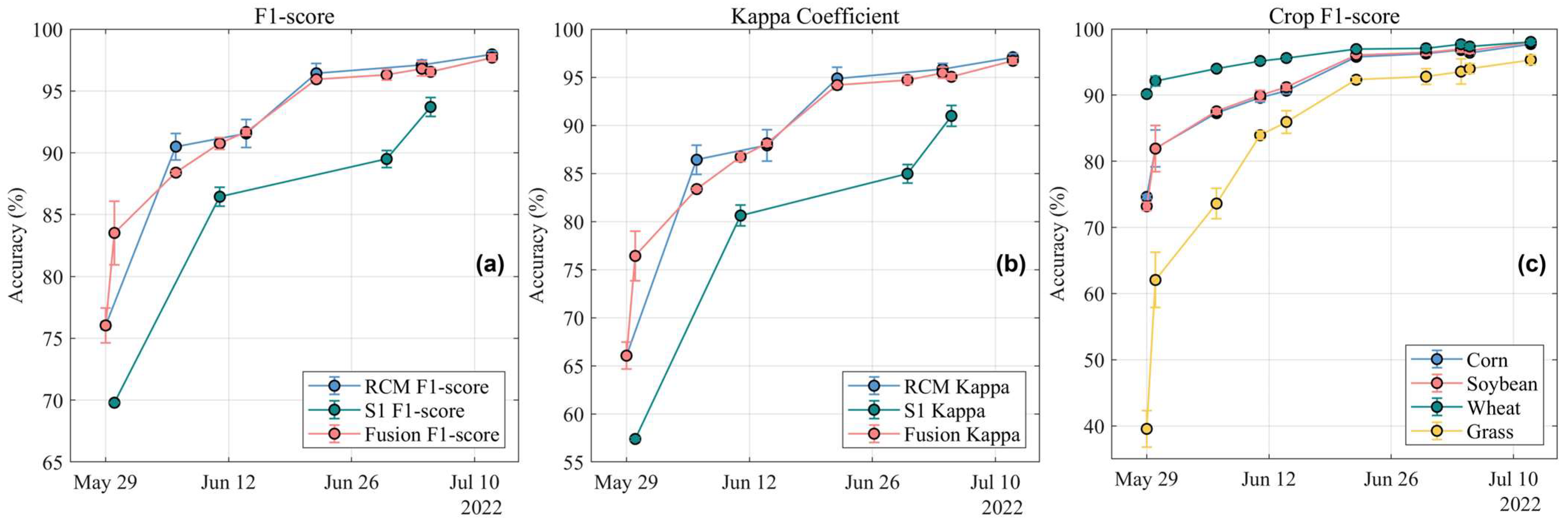
4.3. Accuracy Evaluation in the Early Season

Another objective of this study is to explore two SAR sensors including RCM and Sentinel-1 for early-season crop classification and to monitor the evaluation of the accuracy of crop classification in the early crop growth stages. Using the incremental classification scheme based on the LWAT, which achieved the best results among eight selected methods, every new SAR acquisition, either the Sentinel-1 or RCM (Table 1), triggers a new model training and prediction of crop maps.
The classification results using the incremental procedure with both RCM and Sentinel-1 time-series data are shown in Figure 7. Overall, with an increase in SAR data, the occurrence of misclassified small patches in the classification results has been depressed gradually, leading to smoother classification outcomes. Using only a single-scene RCM image for crop identification on 29 May yielded reasonably accurate crop maps. Nevertheless, due to the limited time-series information, there was space for improvement in the classification results. Subsequently, the integration of a Sentinel-1 image into the results on 30 May resulted in an increased number of small patches compared to the previous phase, especially for the corn and soybean categories. This addition significantly enhanced the ability to distinguish grassland from other crop types.
The results are further illustrated through precision metrics, including F1-score and Kappa, as presented in Figure 8. In Figure 8a,b, whether employing a combination of RCM and Sentinel-1 data or relying solely on RCM, the precision metrics demonstrate a noticeable upward trend until approximately 20 June, which was followed by a sustained plateau consistently exceeding 95%. In contrast, the precision associated with the exclusive utilization of Sentinel-1 data did not reach saturation by that specified date. Convergence with the precision of RCM data was observed exclusively during the final phase of the imaging sequence when using a single dataset. It is noteworthy that the accuracy achieved using RCM alone was comparable to that achieved by utilizing both datasets. However, in the early season, dense data facilitated the generation of acceptable crop maps earlier, starting from 30 May. Additionally, the accuracy of RCM consistently outperformed that of Sentinel-1 in the early season even with an equivalent number of SAR images.
Figure 8c presents the changes in the accuracy of three major crops as well as the grass class in the study area. The wheat exhibited higher accuracy than other crops earlier due to its advanced phenological stages, facilitating its identification from other crops. Regarding soybeans and corn, the initial accuracy, standing at approximately 74%, rose to 82% on 30 May with the addition of Sentine-1 data. Subsequently, accuracy gains persisted in tandem with cumulative data acquisition, culminating in a stabilized precision over 97%. A marked surge in accuracy is conspicuously observed for the grass category, ascending from an initial 40% to a remarkable 92% by 22 June. During the same period, corn and soybean accuracy exhibited an appreciable surge of approximately 21%. Generally, 22 June marks a critical juncture, ensuring the availability of a sufficient volume of SAR images and yielding commendable classification outcomes in the early season.

5. Discussion

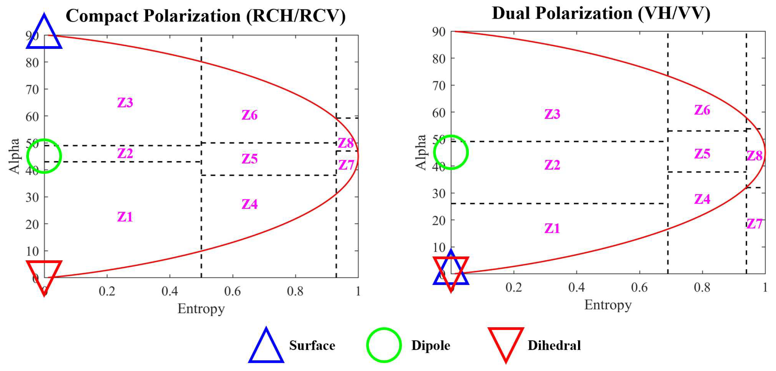
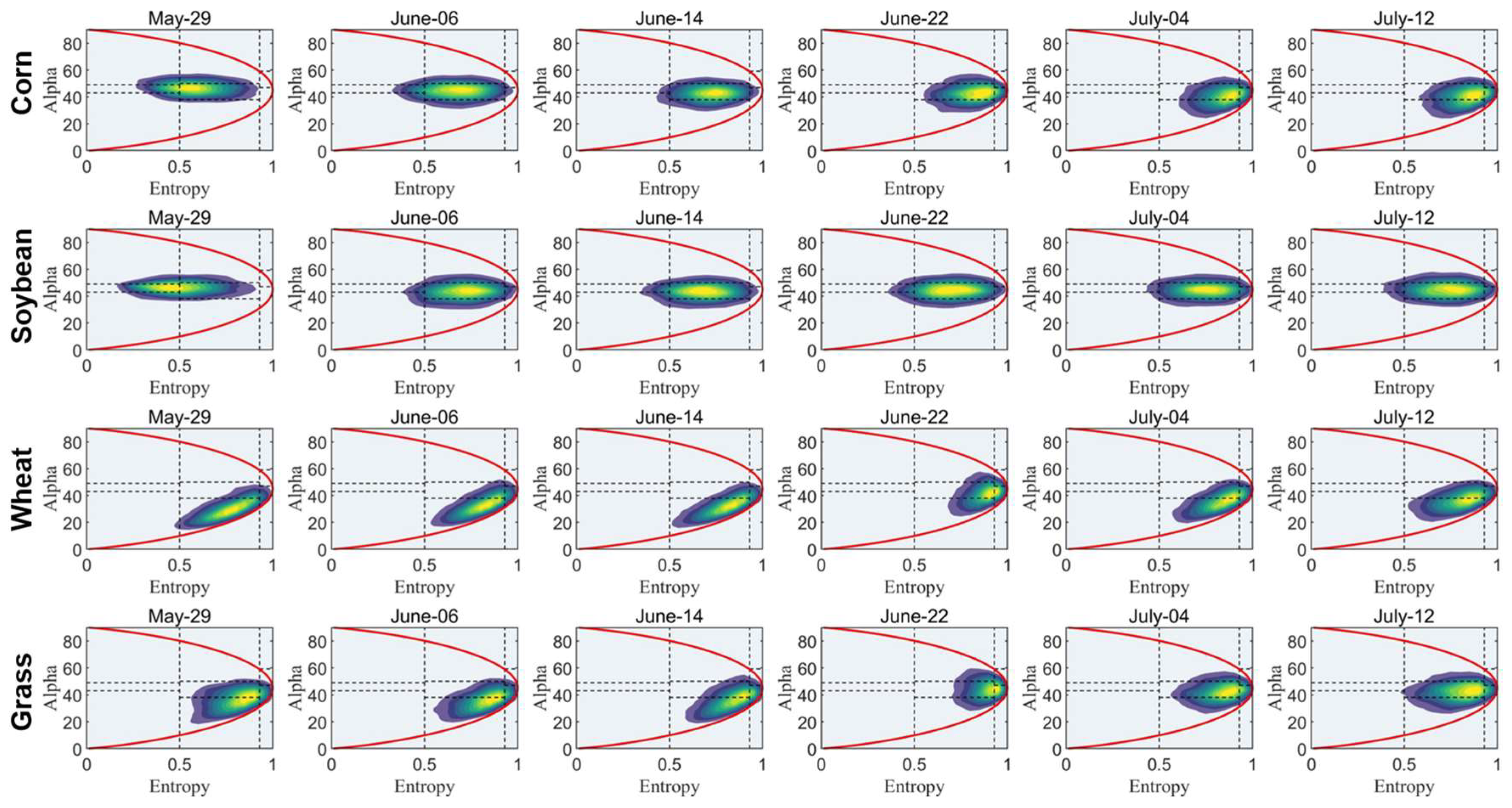
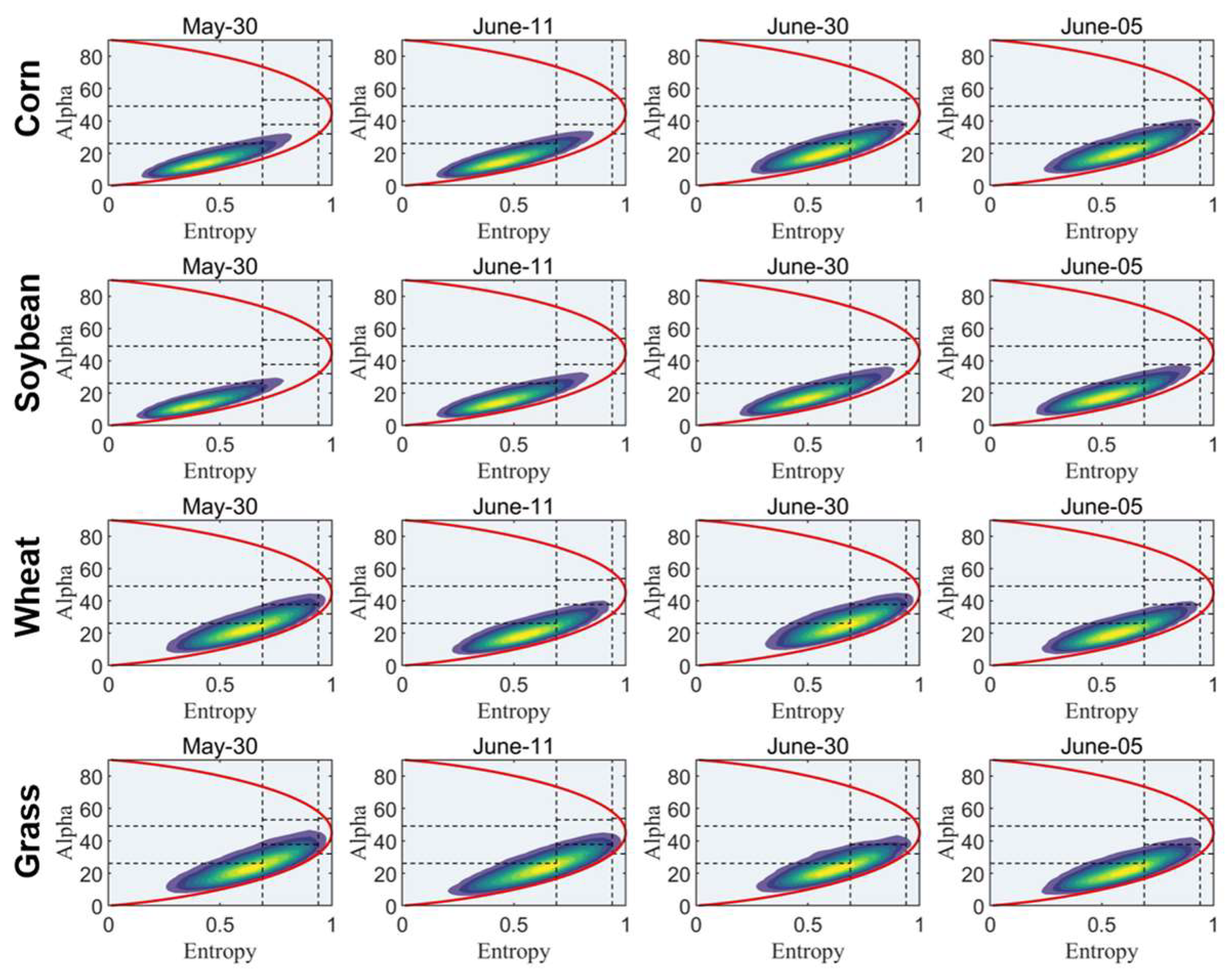
5.1. Feature Analysis of Compact- and Dual-Polarization

According to the accuracy evolution in Figure 8a, RCM outperformed Sentinel-1 in terms of classification accuracy. Due to the both of them being C-band SAR, the major difference between RCM and Sentinel-1 is the polarization mode, i.e., compact polarimetry and dual polarimetry. One of the methods to analyze the physical mechanism behind their ability to discriminate crops is the polarimetric decomposition. In this study, the H/Alpha decomposition was selected to provide clues for analyzing the differences between compact- and dual-polarization SAR [40,41]. The feature plane generated by polarimetric entropy and scattering angle (alpha) was utilized to describe the feature changes of major crops (corn, soybean, wheat, and grass) in the early season, which was divided into several zones to represent different scattering mechanisms [42,43].
Figure 9 presents three canonical scattering mechanisms presented by elementary targets in compact- and dual-polarization entropy/alpha planes. It is noted that the compact-polarization plane can clearly separate dihedral (double-bounce scattering), dipole (volume scattering), and surface targets (surface scattering). However, for linear polarization channels, the HH is sensitive to surface scattering mechanisms such as specular reflection, double bounce, and volume scattering from horizontally oriented structures. Conversely, the VV channel is sensitive to surface scattering mechanisms such as single bounce and volume scattering from vertically oriented structures. Since Sentinel-1 lacks the HH channel, its dual-polarization plane cannot clearly separate surface and dihedral scattering due to it lacking the co-polarization band [43,44].
Figure 10 and Figure 11 are the variation of scattering features derived from RCM and Sentinel-1 in the early season, respectively. In Figure 10, the scatter plot of corn was dominated by mid-entropy dipole scattering at the beginning, and as the crop grew, the polarization entropy increased gradually and moved to dihedral scattering (Z5 to Z7). By contrast, the soybean showed a similar scattering pattern at the beginning, while there was only a slight increase in entropy. However, the distinction between dihedral and surface scattering posed a challenge for Sentinel-1 (Figure 11), resulting in an initial inability to differentiate between soybean and corn during the early stages of growth. As both corn and soybean continued to develop, their scattering plots illustrated a similar progression, slightly shifting from a low-entropy to a mid-entropy zone (from Z1 to Z4).

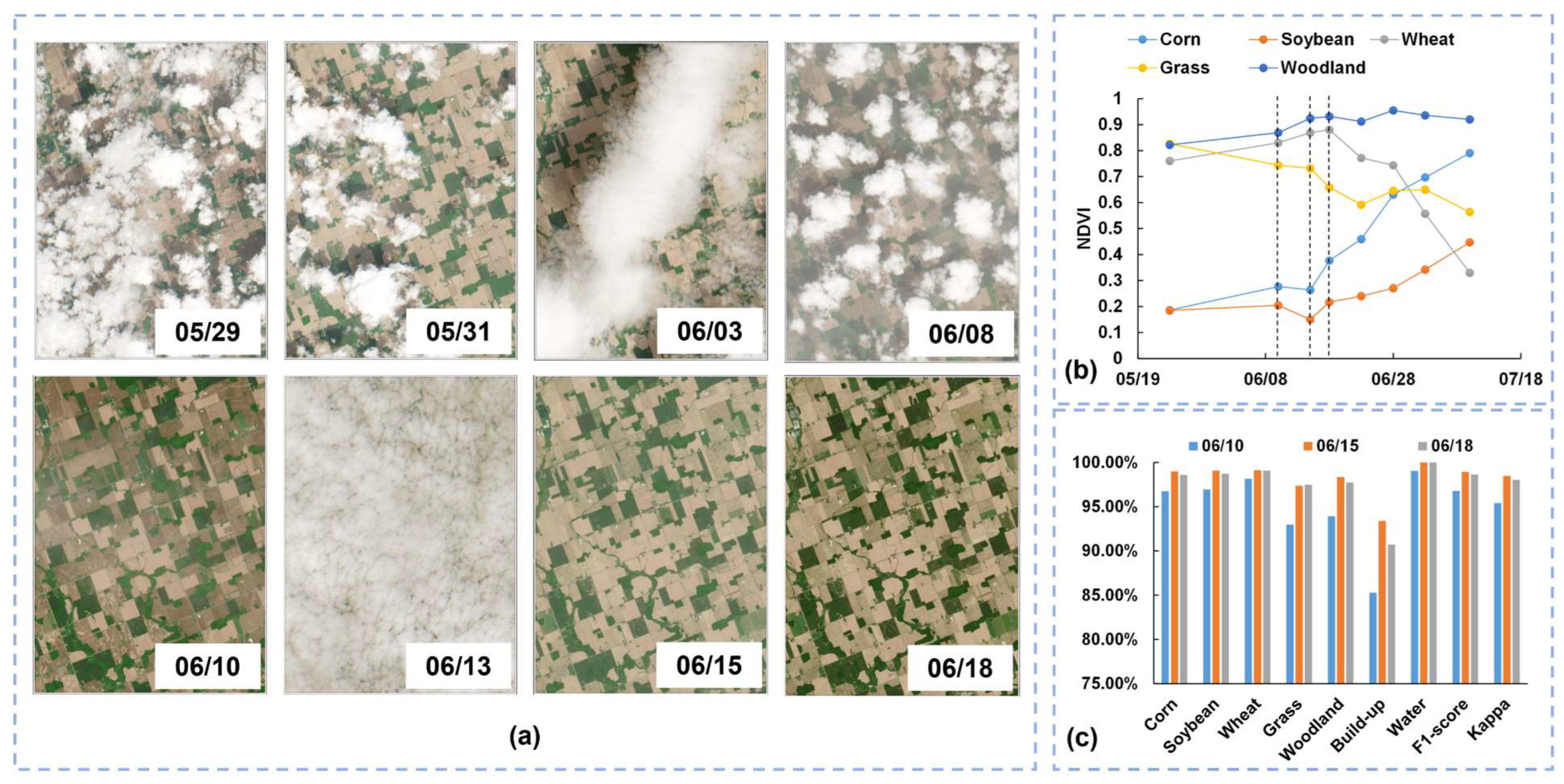
5.2. Compared with Optical Sensors

This section aims to compare the classification performance of SAR data with optical images to highlight the advantages of SAR for early-season crop classification. Here, Sentinel-2 was selected due to its shorter revisit time than Landsat and open access. However, before 10 June, cloud cover and fog significantly hindered the availability of images, as depicted in Figure 12a. During the same period, two scenes of RCM and one scene of Sentinel-1 were collected. Subsequently, an incremental approach was adopted for classification, utilizing Sentinel-2 data from 10 June, 15 June, and 18 June. All spectral bands were employed as inputs for the LWAT classification, and the quantitative assessment outcomes are presented in Figure 12c.
Based on the results in Figure 12c, a remarkable F1-score of 96.78% and a Kappa value of 95.41% were acquired even with just a single Sentinel-2 image. As more images were incorporated, the accuracy consistently improved, surpassing 98%, which is comparable to the accuracy achieved by SAR in early July. Examining the changes in NDVI as illustrated in Figure 12b, there is an approximate 0.1 difference in NDVI values between corn and soybean around 10 June. This disparity widens as the crops mature. Sentinel-2 effectively capitalizes on these spectral distinctions, enabling successful differentiation between the two crops. The experiment underscores the capability of optical satellites to discriminate between crop types in the early stages of the growing season, aligning with previous research findings [18,19]. In contrast, dense SAR data by integrating Sentinel-1 and RCM can provide reliable prior information for decision making at the beginning of crop growth, which is earlier than previously reported [9,14,19,22]. At the same time, SAR can achieve similar accuracy to optical images through the accumulation of data.

5.3. Optimal Phenological Stage for Early-Season Classification

In Figure 8, the classification accuracy for the main crops reached a plateau around 22 June. However, when applying this knowledge to a different study site, relying solely on dates becomes less dependable. Instead, a more robust connection between dates and crop phenology is established particularly for corn and soybean. By cross-referencing field photographs (Figure 3) and compiled phenological stages (Table 1), on 14 June, corn had entered the initial stages of stem elongation, while soybean was undergoing side shoot formation. During these phases, a noticeable surge in crop canopy coverage was evident for both corn and soybean. Prior to 14 June, most fields predominantly displayed bare soil, owing to the smaller size of the crop plants. However, by 14 June, the prevailing cover in the fields had transformed into a vegetative canopy. Subsequent to this stage, corn experienced a height increase, leading to conspicuous and easily distinguishable contrasts in the physical appearance of the two crops. Thus, the phenology of stem elongation of corn is an optimal phenological stage for obtaining early-season crop maps. This choice not only yields classification outcomes of satisfactory accuracy but also ensures the attainment of crop maps at the earliest feasible juncture.

6. Conclusions

This study introduced an application framework for early-season crop classification, integrating LWAT with time-series Sentinel-1 and RCM data. Assessing its effectiveness across corn, soybean, and wheat in southwest Ontario, Canada from 29 May to 12 July 2022 revealed the superiority of LWAT. LWAT achieved remarkable F1-scores of 97.96% and 98.07% for the northern and southern crop regions, respectively, leveraging RCM and Sentinel-1 data. The study highlighted the early-stage performance advantage of RCM over Sentinel-1 and demonstrated the potential of SAR images for early-season crop mapping. Identifying the optimal date for acceptable crop mapping results from SAR images, approximately six weeks after seeding, emphasized the importance of stem elongation of corn. This study underscores the potential of RCM data for timely and dependable information, aiding in-season production forecasting and decision making. Future work aims to enhance method efficiency by addressing redundancy in crop category information within field areas.

Author Contributions

Experiment and initial draft preparation, X.Z.; review and editing, J.W., editing and formal analysis of the paper, B.S. and Y.H. All authors have read and agreed to the published version of the manuscript.

Funding

This work was supported by the Natural Science and Engineering Research Council of Canada (NSERC) Discovery Grant (grant number RGPIN-2022-05051) and Mitacs Accelerate Program (IT37219).

Data Availability Statement

Data are contained within the article.

Acknowledgments

The authors thank the Canada Space Agency (CSA) for providing the RCM SAR data and Heather McNairn from Agriculture and Agri-Food Canada (AAFC) for her help requesting the data. We would also like to thank Marco Chiu and Naythan Samuda for their work on ground truth data collection.

Conflicts of Interest

The authors declare no conflict of interest.

References

  1. Gao, H.; Wang, C.; Wang, G.; Fu, H.; Zhu, J. A Novel Crop Classification Method Based on ppfSVM Classifier with Time-Series Alignment Kernel from Dual-Polarization SAR Datasets. Remote Sens. Environ. 2021, 264, 112628. [Google Scholar] [CrossRef]
  2. Hoekman, D.H.; Vissers, M.A.M. A New Polarimetric Classification Approach Evaluated for Agricultural Crops. IEEE Trans. Geosci. Remote Sens. 2003, 41, 2881–2889. [Google Scholar] [CrossRef]
  3. Liao, C.; Wang, J.; Huang, X.; Shang, J. Contribution of Minimum Noise Fraction Transformation of Multi-Temporal RADARSAT-2 Polarimetric SAR Data to Cropland Classification. Can. J. Remote Sens. 2018, 44, 215–231. [Google Scholar] [CrossRef]
  4. Benami, E.; Jin, Z.; Carter, M.R.; Ghosh, A.; Hijmans, R.J.; Hobbs, A.; Kenduiywo, B.; Lobell, D.B. Uniting Remote Sensing, Crop Modelling and Economics for Agricultural Risk Management. Nat. Rev. Earth Environ. 2021, 2, 140–159. [Google Scholar] [CrossRef]
  5. Huang, X.; Wang, J.; Shang, J.; Liao, C.; Liu, J. Application of Polarization Signature to Land Cover Scattering Mechanism Analysis and Classification Using Multi-Temporal C-Band Polarimetric RADARSAT-2 Imagery. Remote Sens. Environ. 2017, 193, 11–28. [Google Scholar] [CrossRef]
  6. Lobell, D.B.; Thau, D.; Seifert, C.; Engle, E.; Little, B. A Scalable Satellite-Based Crop Yield Mapper. Remote Sens. Environ. 2015, 164, 324–333. [Google Scholar] [CrossRef]
  7. Zhou, X.; Wang, J.; He, Y.; Shan, B. Crop Classification and Representative Crop Rotation Identifying Using Statistical Features of Time-Series Sentinel-1 GRD Data. Remote Sens. 2022, 14, 5116. [Google Scholar] [CrossRef]
  8. Cai, Y.; Guan, K.; Peng, J.; Wang, S.; Seifert, C.; Wardlow, B.; Li, Z. A High-Performance and in-Season Classification System of Field-Level Crop Types Using Time-Series Landsat Data and a Machine Learning Approach. Remote Sens. Environ. 2018, 210, 35–47. [Google Scholar] [CrossRef]
  9. You, N.; Dong, J.; Li, J.; Huang, J.; Jin, Z. Rapid Early-Season Maize Mapping without Crop Labels. Remote Sens. Environ. 2023, 290, 113496. [Google Scholar] [CrossRef]
  10. Becker-Reshef, I.; Franch, B.; Barker, B.; Murphy, E.; Santamaria-Artigas, A.; Humber, M.; Skakun, S.; Vermote, E. Prior Season Crop Type Masks for Winter Wheat Yield Forecasting: A US Case Study. Remote Sens. 2018, 10, 1659. [Google Scholar] [CrossRef]
  11. Gallo, I.; Ranghetti, L.; Landro, N.; La Grassa, R.; Boschetti, M. In-Season and Dynamic Crop Mapping Using 3D Convolution Neural Networks and Sentinel-2 Time Series. ISPRS J. Photogramm. Remote Sens. 2023, 195, 335–352. [Google Scholar] [CrossRef]
  12. You, N.; Dong, J. Examining Earliest Identifiable Timing of Crops Using All Available Sentinel 1/2 Imagery and Google Earth Engine. ISPRS J. Photogramm. Remote Sens. 2020, 161, 109–123. [Google Scholar] [CrossRef]
  13. Skakun, S.; Franch, B.; Vermote, E.; Roger, J.C.; Becker-Reshef, I.; Justice, C.; Kussul, N. Early Season Large-Area Winter Crop Mapping Using MODIS NDVI Data, Growing Degree Days Information and a Gaussian Mixture Model. Remote Sens. Environ. 2017, 195, 244–258. [Google Scholar] [CrossRef]
  14. Dong, J.; Fu, Y.; Wang, J.; Tian, H.; Fu, S.; Niu, Z.; Han, W.; Zheng, Y.; Huang, J.; Yuan, W. Early-Season Mapping of Winter Wheat in China Based on Landsat and Sentinel Images. Earth Syst. Sci. Data 2020, 12, 3081–3095. [Google Scholar] [CrossRef]
  15. Lin, C.; Zhong, L.; Song, X.P.; Dong, J.; Lobell, D.B.; Jin, Z. Early- and in-Season Crop Type Mapping without Current-Year Ground Truth: Generating Labels from Historical Information via a Topology-Based Approach. Remote Sens. Environ. 2022, 274, 112994. [Google Scholar] [CrossRef]
  16. Johnson, D.M.; Mueller, R. Pre-and within-Season Crop Type Classification Trained with Archival Land Cover Information. Remote Sens. Environ. 2021, 264, 112576. [Google Scholar] [CrossRef]
  17. Zhang, C.; Di, L.; Hao, P.; Yang, Z.; Lin, L.; Zhao, H.; Guo, L. Rapid In-Season Mapping of Corn and Soybeans Using Machine-Learned Trusted Pixels from Cropland Data Layer. Int. J. Appl. Earth Obs. Geoinf. 2021, 102, 102374. [Google Scholar] [CrossRef]
  18. Inglada, J.; Vincent, A.; Arias, M.; Marais-Sicre, C. Improved Early Crop Type Identification by Joint Use of High Temporal Resolution SAR and Optical Image Time Series. Remote Sens. 2016, 8, 362. [Google Scholar] [CrossRef]
  19. Jiang, H.; Li, D.; Jing, W.; Xu, J.; Huang, J.; Yang, J.; Chen, S. Early Season Mapping of Sugarcane by Applying Machine Learning Algorithms to Sentinel-1A/2 Time Series Data: A Case Study in Zhanjiang City, China. Remote Sens. 2019, 11, 861. [Google Scholar] [CrossRef]
  20. Marais Sicre, C.; Inglada, J.; Fieuzal, R.; Baup, F.; Valero, S.; Cros, J.; Huc, M.; Demarez, V. Early Detection of Summer Crops Using High Spatial Resolution Optical Image Time Series. Remote Sens. 2016, 8, 591. [Google Scholar] [CrossRef]
  21. Zhao, H.; Chen, Z.; Jiang, H.; Jing, W.; Sun, L.; Feng, M. Evaluation of Three Deep Learning Models for Early Crop Classification Using Sentinel-1A Imagery Time Series-a Case Study in Zhanjiang, China. Remote Sens. 2019, 11, 2673. [Google Scholar] [CrossRef]
  22. McNairn, H.; Kross, A.; Lapen, D.; Caves, R.; Shang, J. Early Season Monitoring of Corn and Soybeans with TerraSAR-X and RADARSAT-2. Int. J. Appl. Earth Obs. Geoinf. 2014, 28, 252–259. [Google Scholar] [CrossRef]
  23. Rußwurm, M.; Courty, N.; Emonet, R.; Lefèvre, S.; Tuia, D.; Tavenard, R. End-to-End Learned Early Classification of Time Series for in-Season Crop Type Mapping. ISPRS J. Photogramm. Remote Sens. 2023, 196, 445–456. [Google Scholar] [CrossRef]
  24. Dingle Robertson, L.; McNairn, H.; Jiao, X.; McNairn, C.; Ihuoma, S.O. Monitoring Crops Using Compact Polarimetry and the RADARSAT Constellation Mission. Can. J. Remote Sens. 2022, 48, 793–813. [Google Scholar] [CrossRef]
  25. Mahdianpari, M.; Mohammadimanesh, F.; McNairn, H.; Davidson, A.; Rezaee, M.; Salehi, B.; Homayouni, S. Mid-Season Crop Classification Using Dual-, Compact-, and Full-Polarization in Preparation for the RADARSAT Constellation Mission (RCM). Remote Sens. 2019, 11, 1582. [Google Scholar] [CrossRef]
  26. Jamali, A.; Roy, S.K.; Bhattacharya, A.; Ghamisi, P. Local Window Attention Transformer for Polarimetric SAR Image Classification. IEEE Geosci. Remote Sens. Lett. 2023, 20, 4004205. [Google Scholar] [CrossRef]
  27. Mohammadi, S.; Belgiu, M.; Stein, A. Improvement in Crop Mapping from Satellite Image Time Series by Effectively Supervising Deep Neural Networks. ISPRS J. Photogramm. Remote Sens. 2023, 198, 272–283. [Google Scholar] [CrossRef]
  28. Krishnaswamy Rangarajan, A.; Purushothaman, R. Disease Classification in Eggplant Using Pre-Trained VGG16 and MSVM. Sci. Rep. 2020, 10, 2322. [Google Scholar] [CrossRef] [PubMed]
  29. Zan, X.; Zhang, X.; Xing, Z.; Liu, W.; Zhang, X.; Su, W.; Liu, Z.; Zhao, Y.; Li, S. Automatic Detection of Maize Tassels from UAV Images by Combining Random Forest Classifier and VGG16. Remote Sens. 2020, 12, 3049. [Google Scholar] [CrossRef]
  30. Xu, J.; Zhu, Y.; Zhong, R.; Lin, Z.; Xu, J.; Jiang, H.; Huang, J.; Li, H.; Lin, T. DeepCropMapping: A Multi-Temporal Deep Learning Approach with Improved Spatial Generalizability for Dynamic Corn and Soybean Mapping. Remote Sens. Environ. 2020, 247, 111946. [Google Scholar] [CrossRef]
  31. Reedha, R.; Dericquebourg, E.; Canals, R.; Hafiane, A. Transformer Neural Network for Weed and Crop Classification of High Resolution UAV Images. Remote Sens. 2022, 14, 592. [Google Scholar] [CrossRef]
  32. Liao, C.; Wang, J.; Xie, Q.; Baz, A.A.; Huang, X.; Shang, J.; He, Y. Synergistic Use of Multi-Temporal RADARSAT-2 and VENμS Data for Crop Classification Based on 1D Convolutional Neural Network. Remote Sens. 2020, 12, 832. [Google Scholar] [CrossRef]
  33. Xie, Q.; Wang, J.; Lopez-Sanchez, J.M.; Peng, X.; Liao, C.; Shang, J.; Zhu, J.; Fu, H.; Ballester-Berman, J.D. Crop Height Estimation of Corn from Multi-Year RADARSAT-2 Polarimetric Observables Using Machine Learning. Remote Sens. 2021, 13, 392. [Google Scholar] [CrossRef]
  34. Meier, U. Growth Stages of Mono-and Dicotyledonous Plants; Blackwell: Berlin/Heidelberg, Germany, 1997. [Google Scholar]
  35. Schmidt, K.; Schwerdt, M.; Hajduch, G.; Vincent, P.; Recchia, A.; Pinheiro, M. Radiometric Re-Compensation of Sentinel-1 SAR Data Products for Artificial Biases Due to Antenna Pattern Changes. Remote Sens. 2023, 15, 1377. [Google Scholar] [CrossRef]
  36. Merzouki, A.; McNairn, H. A Hybrid (Multi-Angle and Multipolarization) Approach to Soil Moisture Retrieval Using the Integral Equation Model: Preparing for the RADARSAT Constellation Mission. Can. J. Remote Sens. 2015, 41, 349–362. [Google Scholar] [CrossRef]
  37. Merzouki, A.; McNairn, H.; Powers, J.; Friesen, M. Synthetic Aperture Radar (SAR) Compact Polarimetry for Soil Moisture Retrieval. Remote Sens. 2019, 11, 2227. [Google Scholar] [CrossRef]
  38. Shaw, P.; Uszkoreit, J.; Vaswani, A. Self-Attention with Relative Position Representations. arXiv 2018, arXiv:1803.02155. [Google Scholar]
  39. Mei, X.; Nie, W.; Liu, J.; Huang, K. Polsar Image Crop Classification Based on Deep Residual Learning Network. In Proceedings of the 2018 7th International Conference on Agro-Geoinformatics (Agro-Geoinformatics), Hangzhou, China, 6–9 August 2018; pp. 1–6. [Google Scholar]
  40. Cloude, S. The Dual Polarization Entropy/Alpha Decomposition: A PALSAR Case Study. Sci. Appl. SAR Polarim. Polarim. Interferom. 2007, 644, 2. [Google Scholar]
  41. Cloude, S.R.; Goodenough, D.G.; Chen, H. Compact Decomposition Theory. IEEE Geosci. Remote Sens. Lett. 2011, 9, 28–32. [Google Scholar] [CrossRef]
  42. Zhang, H.; Xie, L.; Wang, C.; Wu, F.; Zhang, B. Investigation of the Capability of H-Alpha Decomposition of Compact Polarimetric SAR. IEEE Geosci. Remote Sens. Lett. 2013, 11, 868–872. [Google Scholar] [CrossRef]
  43. Ji, K.; Wu, Y. Scattering Mechanism Extraction by a Modified Cloude-Pottier Decomposition for Dual Polarization SAR. Remote Sens. 2015, 7, 7447–7470. [Google Scholar] [CrossRef]
  44. Gella, G.W.; Bijker, W.; Belgiu, M. Mapping Crop Types in Complex Farming Areas Using SAR Imagery with Dynamic Time Warping. ISPRS J. Photogramm. Remote Sens. 2021, 175, 171–183. [Google Scholar] [CrossRef]
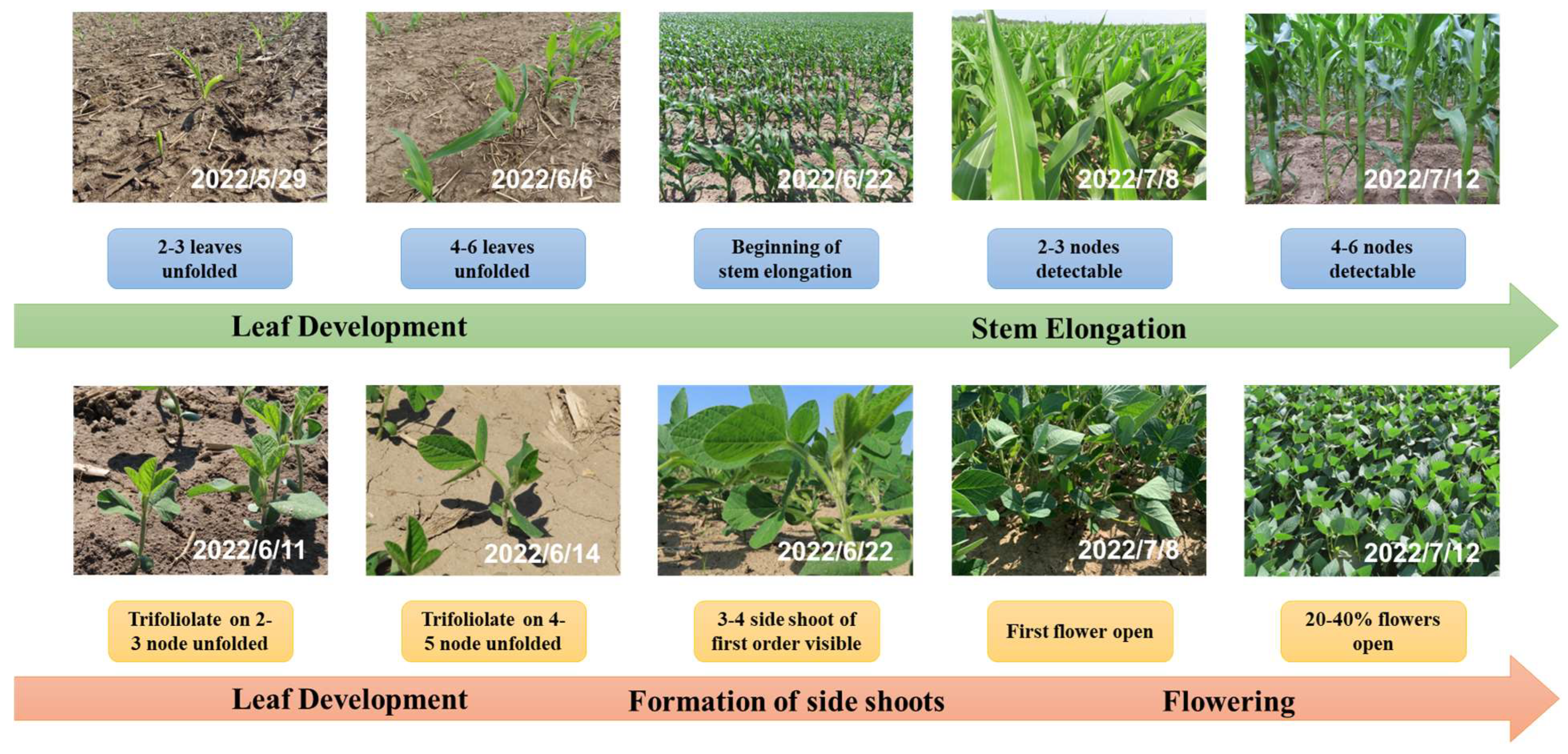
Figure 1. The locations of the study area, which are near the London City, southwest Ontario, Canada.
Remotesensing 16 01376 g001
Figure 2. Ground truth maps of crop types generated by ground survey and visual interpretation. (a) Northern crop region; (b) southern crop region.
Remotesensing 16 01376 g002
Figure 3. Field photos for corn and soybean in the early season.
Remotesensing 16 01376 g003
Figure 4. The flowchart of the framework by integrating the LWAT with time-series RCM and Sentinel-1. It consists of three main parts, pre-processing, feature extractor and local window attention.
Remotesensing 16 01376 g004
Figure 5. Crop classification maps of the north crop region determined by eight methods. (a) SVM; (b) RF; (c) VGG-16; (d) AlexNet; (e) 2DCNN; (f) ResNet-50; (g) ST; (h) LWAT.
Remotesensing 16 01376 g005
Figure 6. Crop classification maps for the southern crop region determined by different deep learning models. (a) VGG-16; (b) AlexNet; (c) 2DCNN; (d) ResNet-50; (e) ST; (f) LWAT.
Remotesensing 16 01376 g006
Figure 7. Classification results using incremental procedure with time-series RCM and Sentinel-1 data for the northern crop region.
Remotesensing 16 01376 g007
Figure 8. The classification accuracy evolution using the incremental procedure in the early season. The X-axis represents the cut-off date of the image acquisition. (a) The evolution of the F1-score; (b) the evolution of the Kappa coefficient; (c) the evolution of major crops in the early season.
Remotesensing 16 01376 g008
Figure 9. Three canonical scattering mechanisms presented by elementary targets in compact- and dual-polarization entropy/alpha planes.
Remotesensing 16 01376 g009
Figure 10. Variation of scattering features of different crops in RCM images with crop growth.
Remotesensing 16 01376 g010
Figure 11. Variation of scattering features of different crops in Sentinel-1 images with crop growth.
Remotesensing 16 01376 g011
Figure 12. (a) Sentinel-2 images covering the study area in the early season; (b) NDVI variation during the early-season period; (c) classification accuracy using Sentinel-2 images.
Remotesensing 16 01376 g012
Table 1. The list of Sentinel-1 and RCM image acquisition.
Acquisition Dates (2022)SatelliteCorn Growth StageSoybean Growth Stage
29 MayRCM2–3 leaves unfoldedFirst pair true leaves unfolded
30 MaySentinel-12–3 leaves unfoldedFirst pair true leaves unfolded
6 JuneRCM4–6 leaves unfoldedFirst pair true leaves unfolded
11 JuneSentinel-16–8 leaves unfoldedTrifoliolate on 2–3 nodes unfolded
14 JuneRCMBeginning of stem elongationTrifoliolate on 4–5 nodes unfolded
22 JuneRCMBeginning of stem elongation3–4 side shoots visible
30 JuneSentinel-1First node detectable7–8 side shoots visible
4 JulyRCM1–2 nodes detectableHarvestable vegetative plant parts final
5 JulySentinel-11–2 nodes detectableHarvestable vegetative plant parts final
12 JulyRCM4–6 nodes detectable20–40% flowers open
Table 2. The quantitative evaluation of crop classification for the north crop region.
SVM (%)RF (%)VGG-16 (%)AlexNet (%)2DCNN (%)ResNet-50 (%)ST (%)LWAT (%)
Corn84.21 ± 0.0282.48 ± 0.0297.57 ± 0.1795.68 ± 0.2797.40 ± 0.0597.70 ± 0.7996.16 ± 0.0497.99 ± 0.31
Soybean83.47 ± 0.0281.97 ± 0.0197.84 ± 0.1896.26 ± 0.2597.63 ± 0.0397.92 ± 0.6996.67 ± 0.0398.13 ± 0.25
Wheat88.23 ± 0.0987.53 ± 0.0198.15 ± 0.0796.20 ± 0.2297.79 ± 0.0698.17 ± 0.6796.94 ± 0.0598.33 ± 0.28
Grass58.58 ± 0.2654.40 ± 0.2496.44 ± 0.2990.50 ± 0.0294.93 ± 0.2496.65 ± 1.1192.74 ± 0.1596.23 ± 0.70
Woodland72.74 ± 0.0970.26 ± 0.0997.30 ± 0.3295.83 ± 0.3297.40 ± 0.0597.23 ± 0.8396.60 ± 0.1397.12 ± 0.16
Build-up37.56 ± 1.5028.81 ± 0.5082.49 ± 5.5459.95 ± 3.7481.32 ± 3.8480.13 ± 6.9276.90 ± 0.7684.68 ± 2.66
Water79.20 ± 0.9178.61 ± 0.6998.10 ± 0.7192.90 ± 0.9396.95 ± 0.4798.88 ± 0.3896.17 ± 0.1494.85 ± 2.89
F1-score83.08 ± 0.0381.48 ± 0.0197.68 ± 0.1695.69 ± 0.2497.42 ± 0.0197.77 ± 0.7596.32 ± 0.0497.96 ± 0.28
Kappa75.81 ± 0.0573.57 ± 0.0196.67 ± 0.2293.82 ± 0.3596.29 ± 0.0296.79 ± 1.0894.72 ± 0.0697.08 ± 0.40
Table 3. The quantitative evaluation of crop classification for the south crop region.
VGG-16 (%)AlexNet (%)2DCNN (%)ResNet-50 (%)ST (%)LWAT (%)
Corn96.98 ± 0.5397.61 ± 0.5697.08 ± 0.3797.38 ± 0.8994.19 ± 1.3798.42 ± 0.28
Soybean95.98 ± 0.7796.80 ± 0.7496.06 ± 0.4996.44 ± 1.2292.66 ± 2.8397.90 ± 0.40
Wheat97.44 ± 0.1297.84 ± 0.6297.66 ± 0.0997.92 ± 0.7095.53 ± 0.9698.28 ± 0.29
Grass96.17 ± 0.1796.93 ± 0.6295.76 ± 0.2296.43 ± 1.0591.46 ± 0.8597.21 ± 0.48
Woodland96.04 ± 0.1396.71 ± 0.3096.18 ± 0.2996.61 ± 0.7695.30 ± 0.7997.16 ± 0.33
Build-up93.65 ± 0.9294.68 ± 0.1693.85 ± 0.1094.22 ± 1.5285.10 ± 6.3496.04 ± 0.75
Water91.37 ± 0.7793.74 ± 2.7594.45 ± 1.1796.05 ± 1.5990.68 ± 4.2196.76 ± 1.29
F1-score96.52 ± 0.5297.22 ± 0.6296.59 ± 0.3796.95 ± 1.0193.58 ± 1.9198.07 ± 0.34
Kappa94.62 ± 0.8195.71 ± 0.9694.73 ± 0.5795.29 ± 1.5690.20 ± 3.1697.02 ± 0.52
Disclaimer/Publisher’s Note: The statements, opinions and data contained in all publications are solely those of the individual author(s) and contributor(s) and not of MDPI and/or the editor(s). MDPI and/or the editor(s) disclaim responsibility for any injury to people or property resulting from any ideas, methods, instructions or products referred to in the content.

