Range-Doppler-Time Tensor Processing for Deep-Space Satellite Characterization Using Narrowband Radar ^†

Abstract

There is growing demand for the high-fidelity characterization of satellites in Geosynchronous Earth Orbit (GEO) to support Space Domain Awareness (SDA). This is particularly true for newly launched satellites, where it is necessary for satellite providers to ascertain whether components have deployed properly. Conventional wideband radar systems are capable of imaging satellites provided that (i) they have sufficient power aperture and bandwidth, and (ii) they observe enough target aspect change to generate a resolved image. While wideband radars are used routinely for characterizing satellites in Low-Earth Orbit (LEO), powerful radars with sensitivity sufficient for large GEO ranges (36,000 km or greater) are lacking. Thus, researchers often rely on more widely available high-power narrowband tracking radars for GEO characterization. In this paper, we present a novel range-Doppler-time (RDT) tensor processing technique for GEO characterization with narrowband radar. This technique encapsulates the strengths of previously proposed methods for narrowband-radar characterization at GEO, providing a generalized approach that can be applied in a variety of settings. The technique generates fully resolved 2D images of rotating GEO satellites in low-bandwidth scenarios. In cases where aspect change is limited, the technique provides detailed Doppler information for enhanced satellite status monitoring. This work presents a comprehensive quantitative analysis of the technique that considers the impact of key parameters on characterization performance. Simulated radar data, and radar data collected in a compact range on a scaled satellite model, are used to evaluate the technique.

1. Introduction

There is a need for detailed characterization of satellites in Geosynchronous Earth Orbit (GEO) to support Space Domain Awareness (SDA). SDA objectives such as satellite stability assessment and target-size estimation are of great interest to the space surveillance community. In addition, satellite providers need to ascertain whether components such as solar panels have deployed properly after launch. Although a number of concepts have been proposed for space–object characterization, ground-based optics and radars are the dominant sensor approaches utilized for this awareness at GEO. Earth-based radars are particularly well matched to satellite characterization, as they can provide high-resolution imagery of space objects at all times of the day and in a variety of weather conditions [1]. Additionally, in contrast to optical sensors, radar image resolution depends only on the transmitted bandwidth and the total aspect change observed, and thus, is independent of the range to the target [2,3]. Ground-based radars can image all satellites visible to the sensor in Low Earth Orbit (LEO) and Medium Earth Orbit (MEO) provided they have sufficient power aperture to generate a detectable return, and thus, they are routinely used for this purpose. However, in GEO, radar imaging is more challenging because, depending on the location of the target, the bandwidth and aspect change needed for high-resolution imaging may not be available. This is due to two factors. First, there are a small number of wideband radars with power sufficient to reach GEO ranges (36,000 km or greater), thus limiting the region of the GEO belt where high range resolution can be achieved. Second, most satellites in GEO are Earth stabilized and reside in low-inclination orbits. Thus, the satellites present very little aspect change to radars on the Earth, resulting in the target being unresolved in cross range.

Related work has explored deep-space satellite characterization through many different approaches, such as light-curve polarimetry for shape and material estimation [4,5], pattern recognition applied to unresolved images for object identification [6], as well as traditional techniques such as frame differencing [7]. Recent efforts have achieved success in applying Artificial Intelligence (AI) algorithms to the problem of SDA, as AI algorithms have proven highly capable of object detection [8]. A recently published paper explored the performance of AI-based algorithms for SDA when compared to legacy methods [9], while other papers have seen success in utilizing AI on light-curve data [10,11,12,13], orbital-observation data [14], or optical imagery [15] for characterization. However, these works do not focus on complex-valued radar data or the capabilities that narrowband imaging offers.

Despite the aforementioned limitations, there are a number of cases where either partial bandwidth or partial aspect change is available, and thus, can be exploited for characterization. There are a large number of deep-space narrowband tracking radars that provide coverage of most of the GEO belt. Thus, researchers often rely on these more widely available high-power radars for GEO characterization. The bandwidth provided by the narrowband radars, while insufficient for traditional high-resolution radar imaging, can be coupled with the Doppler information naturally provided by these sensors to generate images. In addition, satellites present opportunities for imaging when operating in modes where the body rotates, or when the satellite reaches end of life and enters into a tumble motion post-deactivation (after insertion into super-GEO graveyard orbit). Given rotation, Doppler techniques can be used to form resolved images, even in cases where the bandwidth is reduced to the point where the target is unresolved in range. Examples of Doppler techniques applicable to GEO include Doppler–Time Intensity (DTI) analysis [16,17,18,19,20], Doppler tomography imaging [16,17,18,19,21,22,23], coherent narrowband imaging [22,24,25,26,27], and the recently proposed Bandwidth Enhanced Non-coherent Imaging (BENI) algorithm [28].

Doppler–Time Intensity plots, which show the Doppler trajectories of individual scatterers on an object, have long been used to characterize spaceborne targets [1]. More recently, the use of tomography has been explored as a way to generate images of tumbling satellites in the absence of bandwidth [16,28]. Here, each column of the DTI, corresponding to a fixed time instant, provides a one-dimensional projection of the target’s reflectivity. Thus, an inverse Radon transform can be applied to one tumble period of data to form an image of the satellite. As studied in [28], the resulting Doppler tomography images provide a reduced-quality representation of the target in comparison to conventional wideband imaging due to the lack of resolving capability in range from insufficient bandwidth. Noting that many narrowband tracking radars have some bandwidth available, the BENI algorithm was proposed to improve upon Doppler tomography by incorporating range information [28]. For cases where the target has complex rotational dynamics (e.g., spin-precession motion), imaging becomes more challenging. In such cases, the DTI plots by themselves provide valuable information that can be used to make assessments about satellite structure, status, and behavior. Motivated by this, an enhanced DTI product known as Doppler superpulses was developed [16]. Doppler superpulses use information from multiple DTIs (one from each range bin) to form a sensitivity-enhanced composite, which can be used as an input for tomography to produce a superior reconstruction. The utility of the Doppler techniques above was demonstrated for GEO characterization in a recent paper, using multistatic radar data collected on several tumbling space objects. Here, the Millstone Hill radar in Westford, MA and the TIRA radar in Wachtberg, Germany were used as narrowband illuminators with radio telescopes in the United Kingdom and the Netherlands as bistatic receivers [29,30]. These works highlight both the feasibility and successful demonstration of narrowband radar techniques for rotational motion determination and size estimation using real, on-orbit tumbling rocket bodies.

While a number of disparate narrowband-radar techniques have been proposed for GEO characterization, each with strengths in specific scenarios, a generalized processing framework applicable across a variety of settings is lacking. Doppler tomography can be used to image a rotating satellite when the object is unresolved in range (i.e., no or low radar bandwidth). BENI can produce improved images of the same object, but only when additional bandwidth is available. If aspect change is limited, e.g., when only partial rotation of the satellite is observed, one can obtain information through Doppler–time analysis. DTI plots are useful in inferring target type, in determining whether satellite components have deployed properly after launch, and in assessing satellite stability and rotational dynamics. Moreover, DTI plots and tomographic images, in concert, provide complimentary information that can be used to enhance satellite assessment; DTIs capture localized behavior well (e.g., specular reflections, rotational maneuvers), while tomographic images highlight the structural features of targets. Thus, the complete characterization of GEO satellites requires the application of multiple techniques, followed by the interpretation and integration of the data-processing outputs. For robust and efficient characterization at GEO, an integrated processing approach is needed.

In this paper, we present a novel range-Doppler-time (RDT) tensor processing technique for GEO characterization with narrowband radar. This technique encapsulates the strengths of previously proposed methods for narrowband-radar characterization at GEO, providing a generalized approach that can be applied in a variety of settings. Our method expresses the radar signal as a 3D tensor varying in range, Doppler, and time. By applying simple operations to the tensor, we demonstrate that a variety of characterization products can be generated. These include fully resolved 2D power-sum images of rotating GEO satellites, as well as range and Doppler superpulse plots providing detailed, time-localized characterization of space objects. In addition, the 3D framework lends itself well to new extensions of the technique for sensitivity enhancement that exploit the Higher-Order Singular Value Decomposition (HOSVD) of the multi-dimensional tensor. The RDT tensor representation makes it easy to show the relationship between previous processing techniques (e.g., Doppler tomography and BENI) and to understand the impact of key processing parameters.

The goals of this paper are (i) to develop a unified processing technique based on the 3D RDT tensor representation of the radar signal providing enhanced GEO characterization, and (ii) to characterize the performance of the technique as a function of radar and target parameters. Throughout our treatment, we will emphasize challenges encountered when deviating from ideal image models and collection geometries. The key contributions of this work are summarized as follows:

• Development of a novel RDT tensor processing technique for deep-space satellite characterization
• Quantitative performance assessment of the RDT tensor processing technique considering the impact of key parameters on characterization performance
• Demonstration of extensions to the RDT tensor framework, including tensor denoising using the Higher-Order Singular Value Decomposition (HOSVD) to produce enhanced sensitivity images

The organization of this paper is as follows. Section 2 presents the target radar-return signal model and provides a review of standard radar-characterization techniques. Section 3 develops the novel 3D RDT tensor processing technique, presenting results using both simulated and compact-range radar data. Previous imaging algorithms, Doppler tomography and BENI, are presented as related cases of the power-sum imaging method proposed herein. A quantitative performance analysis of the approach is introduced in Section 4. Section 5 discusses extensions of the 3D tensor technique. Conclusions are presented in Section 6.

2. Background on Radar Characterization of Space Objects

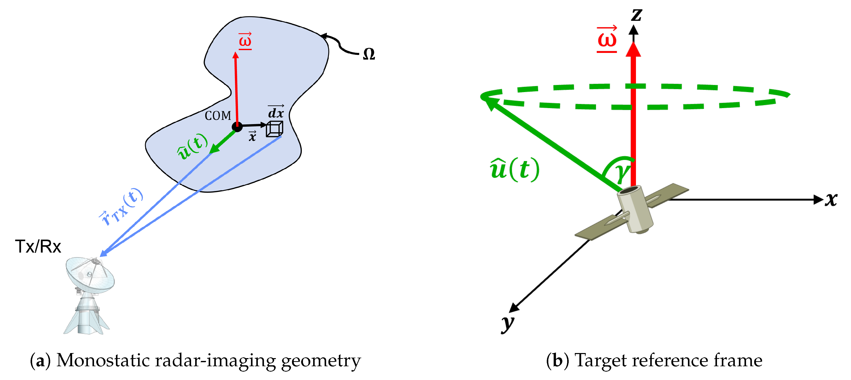
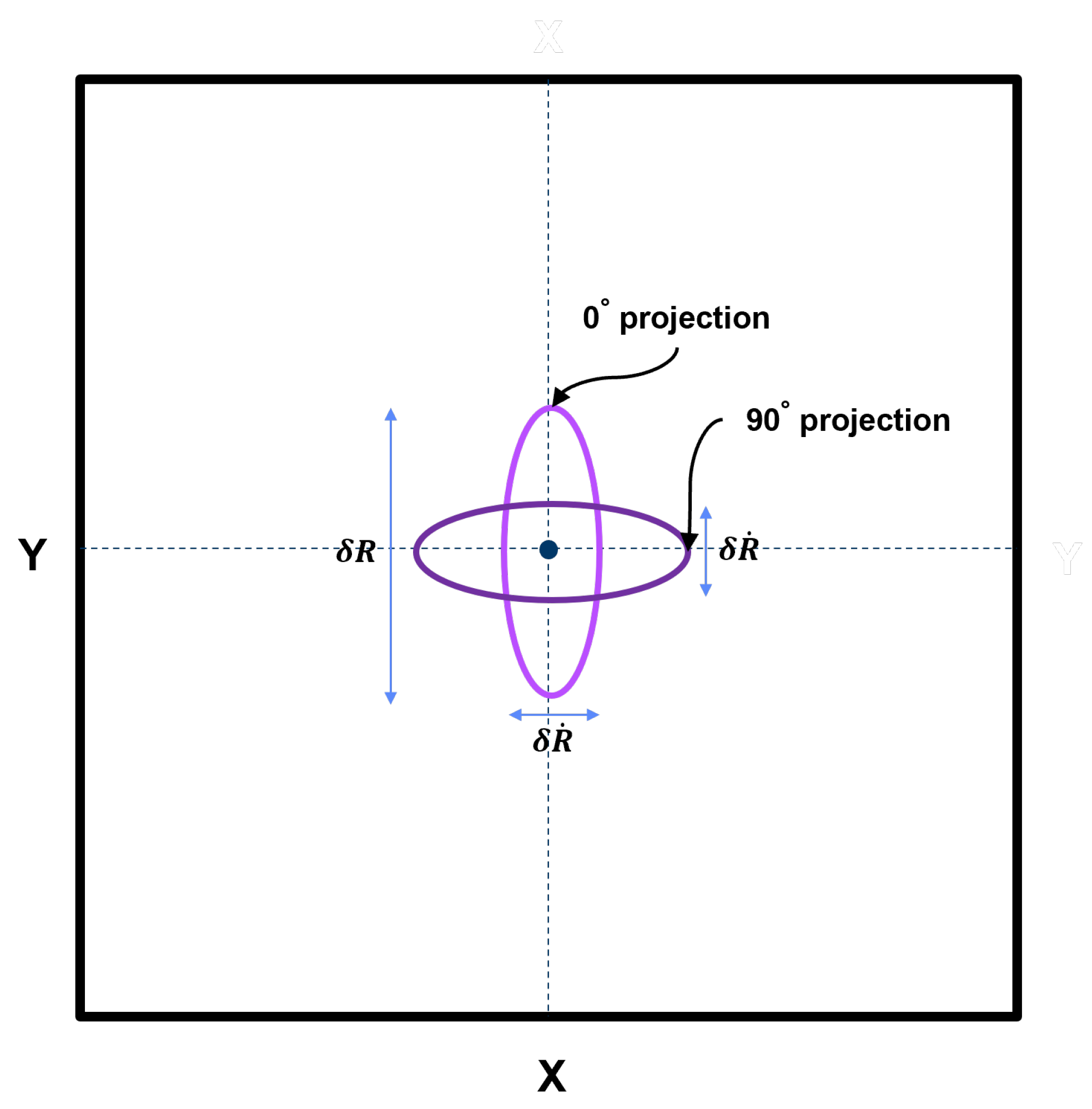
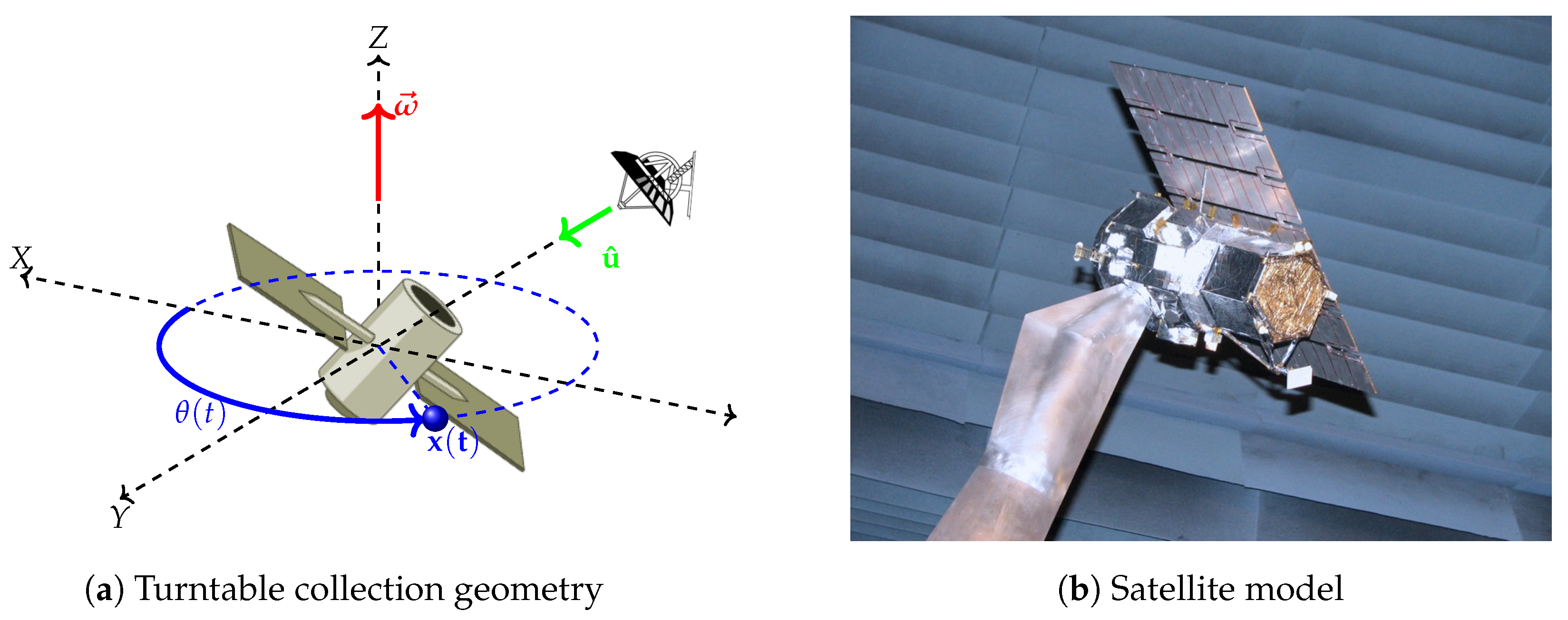
2.1. Radar Imaging Geometry

The derivations for the monostatic radar-return signal models and imaging geometry in our work are based on the following assumptions. We first assume the target is under pure tumbling motion (angular velocity $\overrightarrow{\mathit{\omega }}$ is constant during the entire satellite pass). Previous work on estimating tumble periods of inactive GEO satellites has shown this to be a valid assumption over multiple full rotations of the object [31]. For real on-orbit targets, translational motion compensation is needed to ensure the center of rotation of the object is aligned at zero Doppler [30]. This form of Doppler alignment results in well focused radar-image reconstructions, and thus best serves to maximize image contrast. The uniform rotation of different point scatterers on the target can be represented using a turntable geometry. The target shown in Figure 1a has an angular velocity $\overrightarrow{\mathit{\omega }}$, which is aligned with the Z-axis of the depicted coordinate system fixed to the target’s frame, as shown in Figure 1b.

Using the origin of the target’s frame, we define the radar’s Line-Of-Sight (LOS) as the following time-varying unit vector $\widehat{\mathbf{u}}\left(\mathbf{t}\right)$:

$$\widehat{\mathbf{u}}\left(t\right)=\left[\begin{array}{c}sin\left(\dot{\theta }t\right)sin\gamma \\ cos\left(\dot{\theta }t\right)sin\gamma \\ cos\gamma \end{array}\right]$$

(1)

where $\widehat{\mathbf{u}}\left(\mathbf{t}\right)$ points from the target center of mass to the radar, and

$${\displaystyle \dot{\theta }=\frac{2\pi }{T_p}}$$

denotes the rotation rate of the object tumbling with period $T_p$, and $\gamma$ is the tumble angle between the radar LOS and the target’s rotation axis $\overrightarrow{\omega }$, as shown in Figure 1b. The position of the radar relative to the target’s center of mass is defined as ${\mathbf{r}}_{\mathbf{TX}}\left(\mathbf{t}\right)=r_{TX}\left(t\right)\widehat{\mathbf{u}}\left(\mathbf{t}\right)$. The target can be represented using a complex-valued radar scattering reflectivity density, $\sigma \left(\mathbf{x}\right)$, defined over a spatial volume $\Omega \subset {\mathbb{R}}^3$, where $\mathbf{x}={[x,y,z]}^T\in \Omega$ is the position of a scattering element (or scatterer) on the target. Note that both $\widehat{\mathbf{u}}\left(t\right)$ and $\mathbf{x}$ are expressed in a body-frame coordinate system that is fixed to the target. The target and the coordinate system rotate in a counter-clockwise fashion, which is equivalent to the radar LOS rotating clockwise in the body frame and tracing out a cone.

The absolute monostatic range $\tilde{R}(t;\mathbf{x})$ associated with a scatterer at $\mathbf{x}\in \Omega$ can be computed and approximated as follows:

$$\begin{array}{cc}\hfill \tilde{R}(t;\mathbf{x})& =∥\mathbf{x}-r_{TX}\left(t\right)\widehat{\mathbf{u}}\left(\mathbf{t}\right)∥\hfill \\ \hfill & =r_{TX}\left(t\right)\sqrt{1+\frac{{∥\mathbf{x}∥}^2}{r_{TX}^2\left(t\right)}-\frac{2{\mathbf{x}}^T\widehat{\mathbf{u}}\left(\mathbf{t}\right)}{r_{TX}\left(t\right)}}\hfill \\ \hfill & \approx r_{TX}\left(t\right)\left[1-\frac{{\mathbf{x}}^T{\widehat{\mathbf{r}}}_{\mathbf{TX}}\left(\mathbf{t}\right)}{r_{TX}\left(t\right)}\right]\hfill \\ \hfill & =r_{TX}\left(t\right)-\underset{R(t;\mathbf{x})}{\underbrace{{\mathbf{x}}^T\widehat{\mathbf{u}}\left(\mathbf{t}\right)}},\hfill \end{array}$$

(2)

$$\begin{array}{cc}\hfill R(t;\mathbf{x})& ={\mathbf{x}}^T\widehat{\mathbf{u}}\left(\mathbf{t}\right),\hfill \end{array}$$

(3)

where $R(t;\mathbf{x})$ denotes the relative range, or range to the scattering element at $\mathbf{x}$ relative to the center of mass of the object.

The expression for the scatterer relative-range trajectory in (3) makes several simplifying assumptions that are often applicable to GEO and near-GEO objects. First, the radar and satellite center of mass are fixed relative to each other. This assumption is appropriate for an Earth-based radar observing a satellite in Geosynchronous orbit (i.e., orbit with zero-inclination at GEO altitude). Second, the satellite is in a pure tumble, rotating with a fixed angular velocity. The two assumptions hold reasonably well for slowly drifting objects subject to natural forces over the timescales of interest for imaging. Later in the paper, we will discuss the impact of deviations from the assumptions.

Using (1) and (3), we have

$$R(t;\mathbf{x})=xsin\gamma sin\left(\dot{\theta }t\right)+ysin\gamma cos\left(\dot{\theta }t\right)+zcos\gamma .$$

(4)

To gather more intuition about the form of (4), we express x and y in polar coordinates: $x=\rho cos\phi$ and $y=\rho sin\phi$. This results in

$$R(t;\mathbf{x})=\rho sin\gamma sin(\dot{\theta }t+\phi )+zcos\gamma .$$

Thus, the trajectory takes the form of a sinusoid with amplitude $\rho sin\gamma$, phase angle $\phi$, and offset $zcos\gamma$. Note that the sinusoid attains maximum amplitude when $\gamma =\pi /2$ (radar LOS orthogonal to the rotation axis), and has amplitude zero for $\gamma =0$ (LOS parallel to the rotation axis).

2.2. Radar-Return Signal Model

The radar-return signal model for an object in a pure tumble at GEO is [2]

$${\displaystyle G(f,t)={\int }_{\Omega }\sigma \left(\mathbf{x}\right)exp\left({\displaystyle -j\frac{4\pi }{c}fR(t;\mathbf{x})}\right)d\mathbf{x},}$$

(5)

where

$${\displaystyle f_c-\frac{B}{2}\le f\le f_c+\frac{B}{2}}$$

is frequency, $t\in [0,T_{max}]$ is slow-time, B is the bandwidth transmitted by the radar at center frequency $f_c$, and $\sigma \left(\mathbf{x}\right)$ is the radar reflectivity density at position $\mathbf{x}={[x,y,z]}^T\in \Omega$. We refer to the radar signal in (5), which varies with frequency and time, as the phase-history data.

2.3. Compact-Range Satellite Model Case Study

To validate our methods in this paper, we tested using real compact-range radar data obtained from a scale model of a satellite. The data were collected at the Submillimeter-Wave Technology Laboratory at University of Lowell in their 160 GHz center frequency compact range [32], utilizing the turntable geometry shown in Figure 2a [33]. The model scale factor and center frequency were selected such that the ratio of the center frequency to the scale model is comparable to the full-size object. After collection, the data were scaled to X-band (10 GHz center frequency), resulting in a bandwidth of $B=2\mathrm{GHz}$. The satellite scale model, displayed in Figure 2b, is structurally characterized by its hexagonal bus and segmented solar panels, with etched cells and machined hinges along the frame.

2.4. Standard Radar-Characterization Processing

In this section, we review standard radar-characterization processing techniques. This overview provides necessary background before motivating the generalized 3D RDT technique.

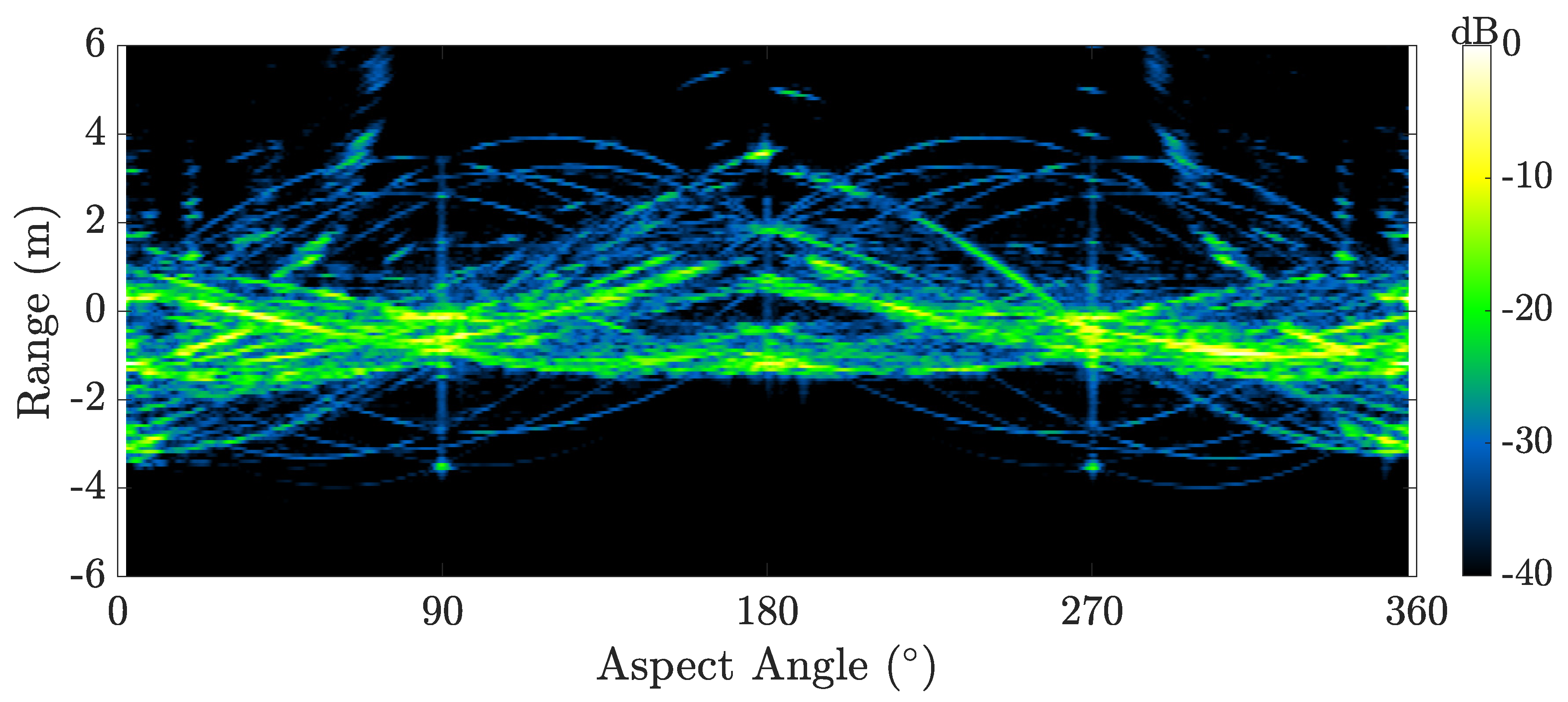
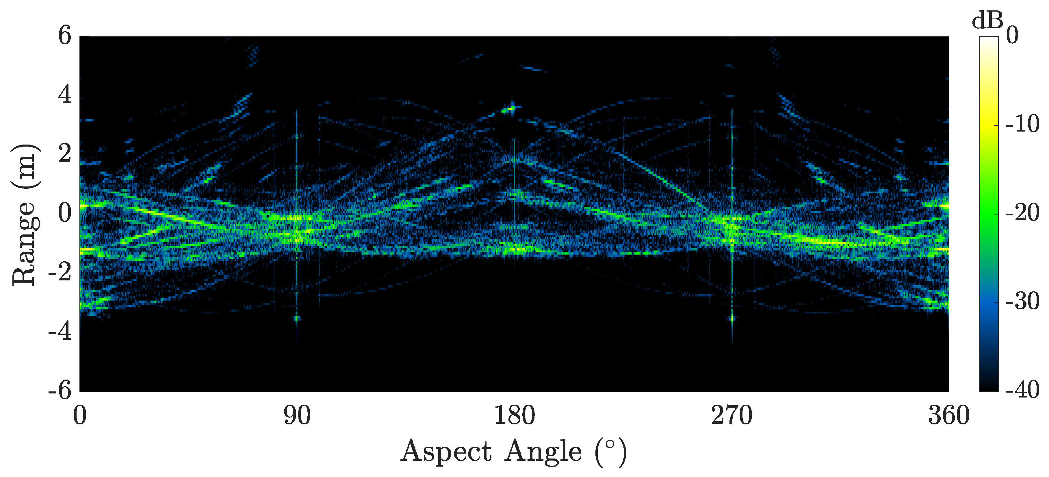
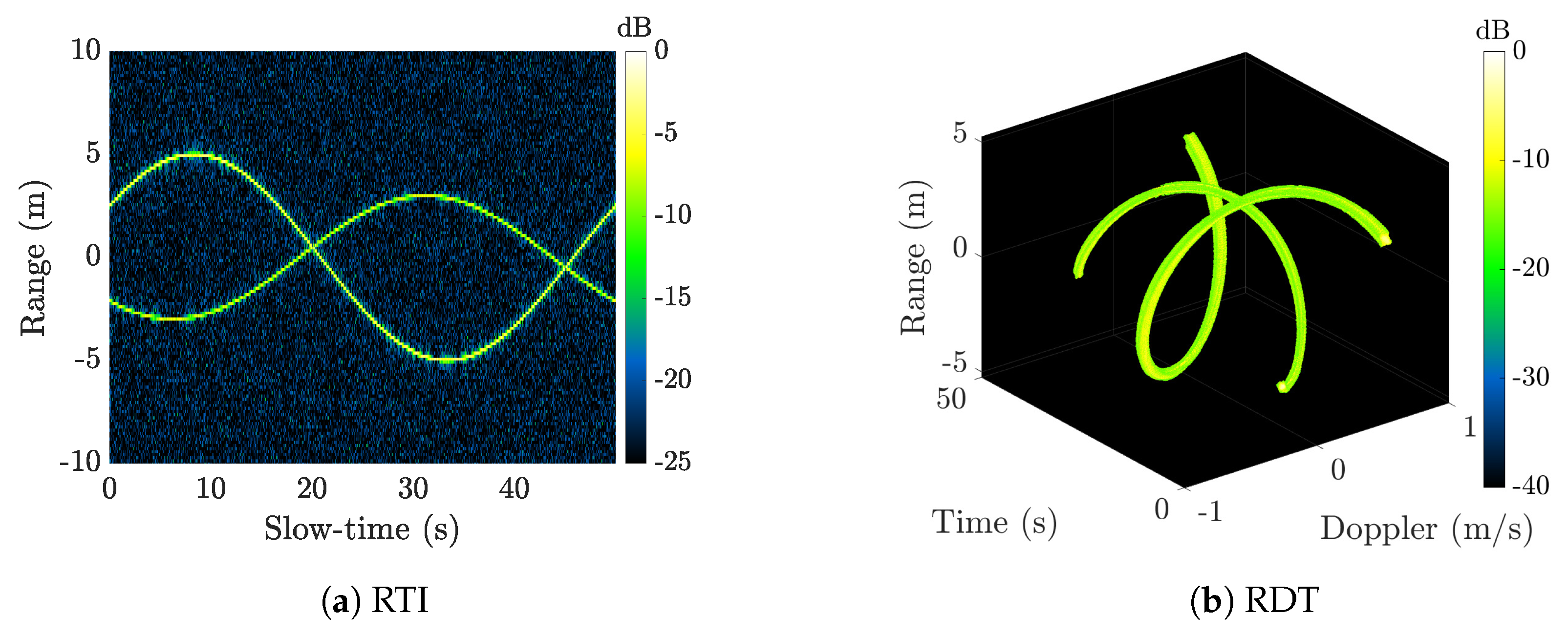
2.4.1. Range–Time Intensity (RTI)

The Range–Time Intensity (RTI) data captures that evolution of the wideband target signature along the radar LOS as a function of time. The RTI data $\widehat{g}(r,t)$ are generated by applying an inverse Fourier transform in frequency to the phase-history data in (5):

$${\displaystyle \widehat{g}(r,t)={\int }_{-B/2}^{B/2}G(f,t)exp\left({\displaystyle j\frac{4\pi }{c}{f}_{B}r}\right)d{f}_B,}$$

(6)

where $f_B$ represents baseband frequency such that $f=f_c+f_B$. Applying (5) to (6) yields

$${\displaystyle \widehat{g}(r,t)=B{\int }_{\Omega }\sigma \left(\mathbf{x}\right)exp\left({\displaystyle -j\frac{4\pi }{c}{f}_{c}R(t;\mathbf{x})}\right)sinc\left({\displaystyle \frac{r-R(t;\mathbf{x})}{c/2B}}\right)d\mathbf{x}.}$$

(7)

Expression (7) shows that each scattering element contributes a sinc point response in range weighted by the reflectivity and a phase term that is proportional the relative range. The scatterers follow sinusoidal trajectories as a function of time.

Note that the RTI data in (7) are complex-valued. Because of this, the log power of (7), $20{log}_{10}\left(\right|\widehat{g}(r,t)\left|\right)$, is typically displayed for visual interpretation. Figure 3 shows the RTI data for the compact-range satellite model introduced in Section 2.3 over a single full rotation. The bandwidth is large enough such that individual point scatterers are well-resolved in range and trace out sinusoidal trajectories over slow-time. Bright specular flashes occur at aspect angle views $\theta =90°\mathrm{and}{270}^{\circ }$.

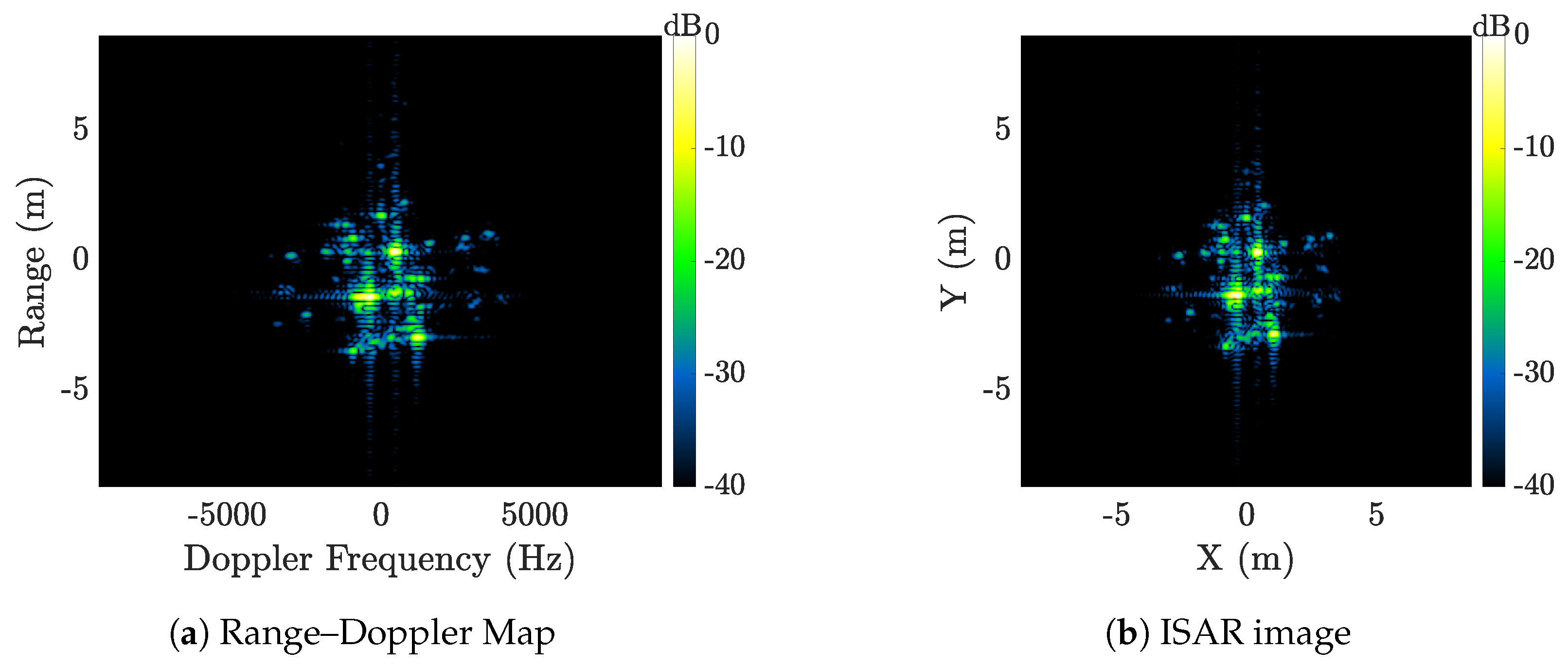
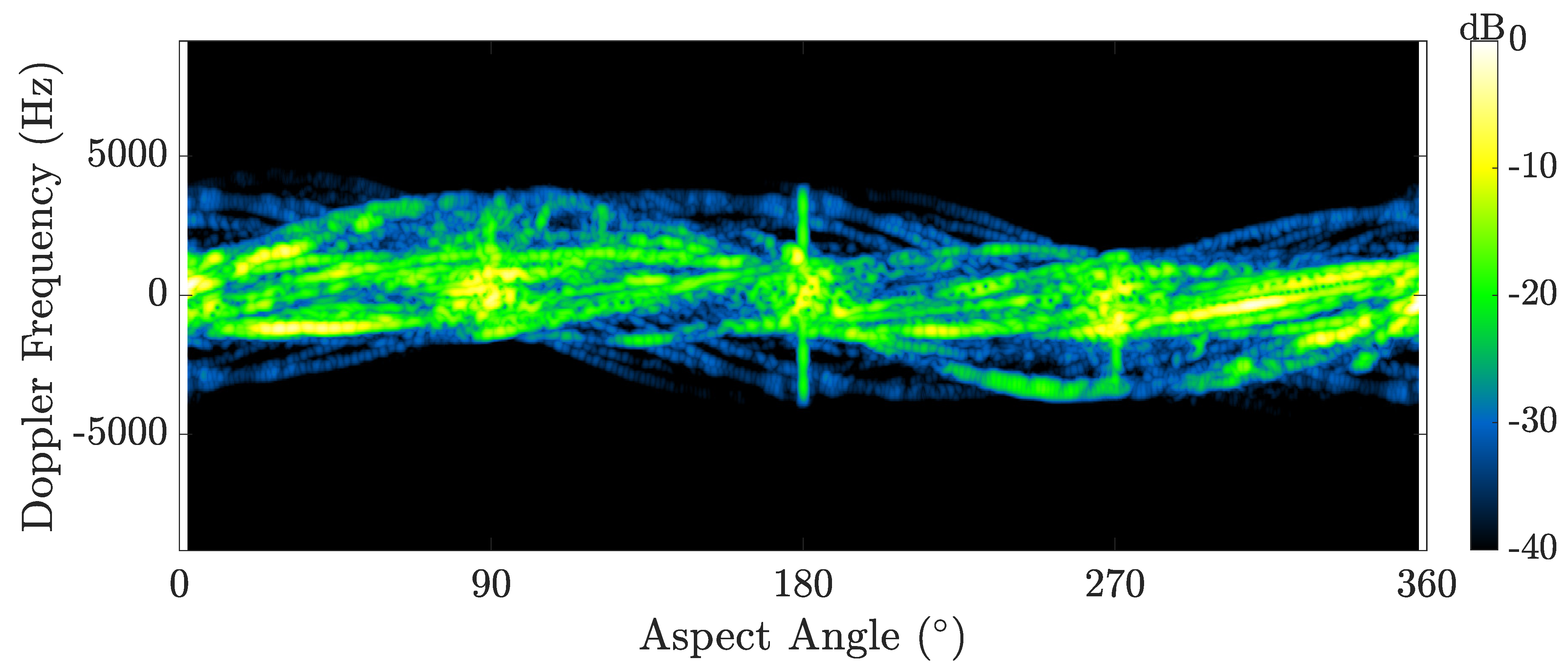
2.4.2. Range–Doppler Map (RDM)

Range–Doppler Maps (RDMs) provide two-dimensional snapshots of rotating objects in range and range rate. Here, Doppler refers to range rate derived from the signal phase. The RDM $g(r,\dot{r})$ is generated by collecting the phase-history data over a window of duration T and applying an inverse 2D Fourier transform:

$${\displaystyle g(r,\dot{r})={\int }_{-T/2}^{T/2}{\int }_{-B/2}^{B/2}G(f,t)exp\left({\displaystyle j\frac{4\pi }{c}{f}_{B}r}\right)exp\left({\displaystyle j\frac{4\pi }{c}{f}_c\overline{t}\dot{r}}\right)d{f}_{B}d\overline{t},}$$

(8)

where $\overline{t}=t-t_i$ is time relative to the window midpoint $t_i$. Let

$${\displaystyle \Phi (f,t)=-\frac{4\pi }{c}fR(t;\mathbf{x})}$$

denote the argument of the phase in (5). Taking a first-order Taylor expansion about $f=f_c$ and $t=t_i$ generates an approximation where the phase is linear in t and f, and is a separable function of the two variables:

$${\displaystyle \Phi (f,t)\approx -\frac{4\pi }{c}fR(t_i;\mathbf{x})-\frac{4\pi }{c}{f}_c\dot{R}(t_i;\mathbf{x})(t-t_i),}$$

(9)

where

$$\dot{R}(t;\mathbf{x})=x\dot{\theta }sin\gamma cos\left(\dot{\theta }t\right)-y\dot{\theta }sin\gamma sin\left(\dot{\theta }t\right)$$

(10)

is the range rate of a scatterer at $\mathbf{x}$. Substitution of (5) and (9) into (8) produces

$${\displaystyle g(r,\dot{r})=BT{\int }_{\Omega }\sigma \left(\mathbf{x}\right)exp\left({\displaystyle -j\frac{4\pi }{c}{f}_{c}R(t;\mathbf{x})}\right)sinc\left({\displaystyle \frac{r-R(t_i;\mathbf{x})}{c/2B}}\right)sinc\left({\displaystyle \frac{\dot{r}-\dot{R}(t_i;\mathbf{x})}{\lambda /2T}}\right)d\mathbf{x}.}$$

(11)

As indicated by (11), RDM processing generates an “image" where each scatterer on the object is rendered as 2D sinc function offset by its range and range rate at time $t_i$. Note that to invoke the approximation in (9), T must be sufficiently small so that higher-order terms in the expansion of t are negligible.

Figure 4a shows a RDM generated from the compact-range dataset using $5^{\circ }$ aspect change and $2\mathrm{GHz}$ bandwidth (scaled to X-band). The RDM reveals the hexagonal bus on the satellite model, with solar panels evident to the left and right of the bus.

2.4.3. Inverse Synthetic Aperture Radar (ISAR) Imaging

The RDM in (11) provides an image of a satellite in the sense that individual scatterers on the object are resolved. For proper image interpretation, we desire a product where scatterers are mapped to their physical positions, and defocusing artifacts due to nonlinearity in the phase are remedied (note that in the approximation in (9), such nonlinearity is assumed to be negligible). Inverse Synthetic Aperture Radar (ISAR) is an approach used to generate a correctly rendered image of the satellite. Like the RDM, an ISAR image is generated by processing a fixed collection window (or integration interval) T centered at a particular time $t_i$. To derive the ISAR imaging equation, we first express (4) in terms of $\overline{t}=t-t_i$:

$$R(\overline{t};\mathbf{x})=xsin\gamma sin(\dot{\theta }\overline{t}+{\theta }_i)+ysin\gamma cos(\dot{\theta }\overline{t}+{\theta }_i)+zcos\gamma ,$$

where ${\theta }_i=\dot{\theta }{t}_i$ is the angle at the center of the interval. By making use of trigonometric identities and rearranging terms, this expression can be represented as

$$R(\overline{t};\mathbf{x})=(xcos{\theta }_i-ysin{\theta }_i)sin\gamma sin\left(\dot{\theta }\overline{t}\right)+(xsin{\theta }_i+ycos{\theta }_i)sin\gamma cos\left(\dot{\theta }\overline{t}\right)+zcos\gamma .$$

(12)

To proceed further, we next consider the special case where $\gamma =\pi /2$, which is the case where the radar LOS is orthogonal to the rotation axis. This removes the dependency upon the height z in (12). Defining the rotated coordinates

$$\begin{array}{cc}\hfill x^{\prime }& =xcos{\theta }_i-ysin{\theta }_i,\hfill \\ \hfill y^{\prime }& =xsin{\theta }_i+ycos{\theta }_i,\hfill \\ \hfill z^{\prime }& =z,\hfill \end{array}$$

we have

$$R(\overline{t};\mathbf{x})=x^{\prime }sin\left(\dot{\theta }\overline{t}\right)+y^{\prime }cos\left(\dot{\theta }\overline{t}\right).$$

Insertion into (5) leads to the ISAR imaging equation

$$\begin{array}{cc}\hfill G(f,\overline{t})& ={\int }_{{\Omega }_x}{\int }_{{\Omega }_y}\left[{\int }_{{\Omega }_z}\sigma (x^{\prime },y^{\prime },z^{\prime })d{z}^{\prime }\right]exp\left(-j2\pi \left[\frac{2f}{c}{x}^{\prime }sin\theta \left(\overline{t}\right)+\frac{2f}{c}{y}^{\prime }cos\theta \left(\overline{t}\right)\right]\right)d{x}^{\prime }d{y}^{\prime }\hfill \\ \hfill & ={\int }_{{\Omega }_x}{\int }_{{\Omega }_y}\overline{\sigma }(x^{\prime },y^{\prime })exp\left(-j2\pi \left[\frac{2f}{c}{x}^{\prime }sin\theta \left(\overline{t}\right)+\frac{2f}{c}{y}^{\prime }cos\theta \left(\overline{t}\right)\right]\right)d{x}^{\prime }d{y}^{\prime },\hfill \end{array}$$

(13)

where

$$\begin{array}{cc}\hfill \overline{\sigma }(x,y)& {\displaystyle ={\int }_{{\Omega }_z}\sigma (x,y,z)dz}\hfill \end{array}$$

(14)

is the projection of the reflectivity function along the z axis.

The phase history data $G(f,\overline{t})$ in (13) has a nice spatial Fourier sampling interpretation. Taking the three-dimensional Fourier transform of the scattering reflectivity function $\sigma (x,y,z)$, we obtain

$$S_{\sigma }(k_x,k_y,k_z)={\int \int \int }_{{\mathbb{R}}^3}\sigma (x,y,z)exp\left(-j2\pi \left[k_{x}x+k_{y}y+k_{z}z\right]\right)dxdydz.$$

(15)

Note that by the Projection Slice Theorem, $S_{\overline{\sigma }}(k_x,k_y)=S_{\sigma }(k_x,k_y,0)$, where $S_{\overline{\sigma }}$ is the 2D Fourier transform of $\overline{\sigma }$. Using this fact, and (13), we can relate $(f,\overline{t})$ samples of the phase-history signal to $S_{\sigma }$:

$$G\left(f,\frac{\theta }{\dot{\theta }}\right)=S_{\sigma }(k_x(f,\theta ),k_y(f,\theta ),0),$$

(16)

where

$$\begin{array}{cc}\hfill k_x(f,\theta )& {\displaystyle =\frac{2f}{c}sin\theta \left(\overline{t}\right),}\hfill \\ \hfill k_y(f,\theta )& {\displaystyle =\frac{2f}{c}cos\theta \left(\overline{t}\right),}\hfill \end{array}$$

are spatial frequencies in the x, y, z dimensions, and $\theta \left(\overline{t}\right)=\dot{\theta }\overline{t}$. Thus, (16) reveals phase-history samples lie on an annular region on the $k_z=0$ plane in the Fourier domain. An image can be reconstructed using a polar integral over the following annular region A:

$$\begin{array}{cc}\hfill \mathrm{g}(x,y)& ={\int \int }_A{S}_{\sigma }(k_x,k_y,0)exp\left(j2\pi \left[k_{x}x+k_{y}y\right]\right)d{k}_{x}d{k}_y\hfill \\ \hfill & ={\int }_{\frac{-\Delta \theta }{2}}^{\frac{\Delta \theta }{2}}{\int }_{2(f_c-B/2)/c}^{2(f_c+B/2)/c}{S}_{\sigma }(k_{r}sin\theta ,k_{r}cos\theta ,0)exp\left(j2\pi \left[k_{r}sin\theta x+k_{r}cos\theta y\right]\right)k_{r}d{k}_{r}d\theta ,\hfill \end{array}$$

(17)

where $\Delta \theta =\dot{\theta }T$ is the integration angle. In Appendix A (Appendix A.1), we show that the image has the form

$$\begin{array}{cc}\hfill \mathrm{g}(x,y)& \approx {\left[\lambda /2\Delta \theta \right]}^{-1}{\left[c/2B\right]}^{-1}{\int }_{{\Omega }_x}{\int }_{{\Omega }_y}\overline{\sigma }(x^{\prime },y^{\prime })exp\left(\frac{-j4\pi f_c{y}^{\prime }}{c}\right)\hfill \\ \hfill & \times sinc\left({\displaystyle \frac{x-x^{\prime }}{\lambda /2\Delta \theta }}\right)sinc\left({\displaystyle \frac{y-y^{\prime }}{c/2B}}\right)d{x}^{\prime }d{y}^{\prime }.\hfill \end{array}$$

(18)

Note $\mathrm{g}(x,y)$ computed in (18) has the same units as $\overline{\sigma }(x,y)$. Thus, the ISAR image computed in (18) is a two-dimensional projection of the three-dimensional reflectivity function onto the $z^{\prime }=0$ plane, where the object is rotated about the rotation axis by ${\theta }_i$.

For the general case where $\gamma <\pi /2$, the imaging relationship cannot be described exactly by a 2D Fourier transform because of the $zcos\gamma$ term in (12). When forming an image using (17), the non-zero z term causes a depth-of-focus effect where scatterers with $z\ne 0$ appear defocused. We will analyze this effect in more detail later in the paper when discussing the limitations of the RDT technique. A slant-plane image can be formed when $\gamma <\pi /2$, where the image is a projection of the 3D reflectivity onto the tangent plane of the cone traced out by the radar line of sight. We derive expressions for the slant-plane image in Appendix A.2.

Figure 4 compares and contrasts RDM and ISAR image reconstructions for the same compact-range dataset. Both results shown in Figure 4a,b are generated using $5^{\circ }$ worth of aspect change and $2\mathrm{GHz}$ of bandwidth.

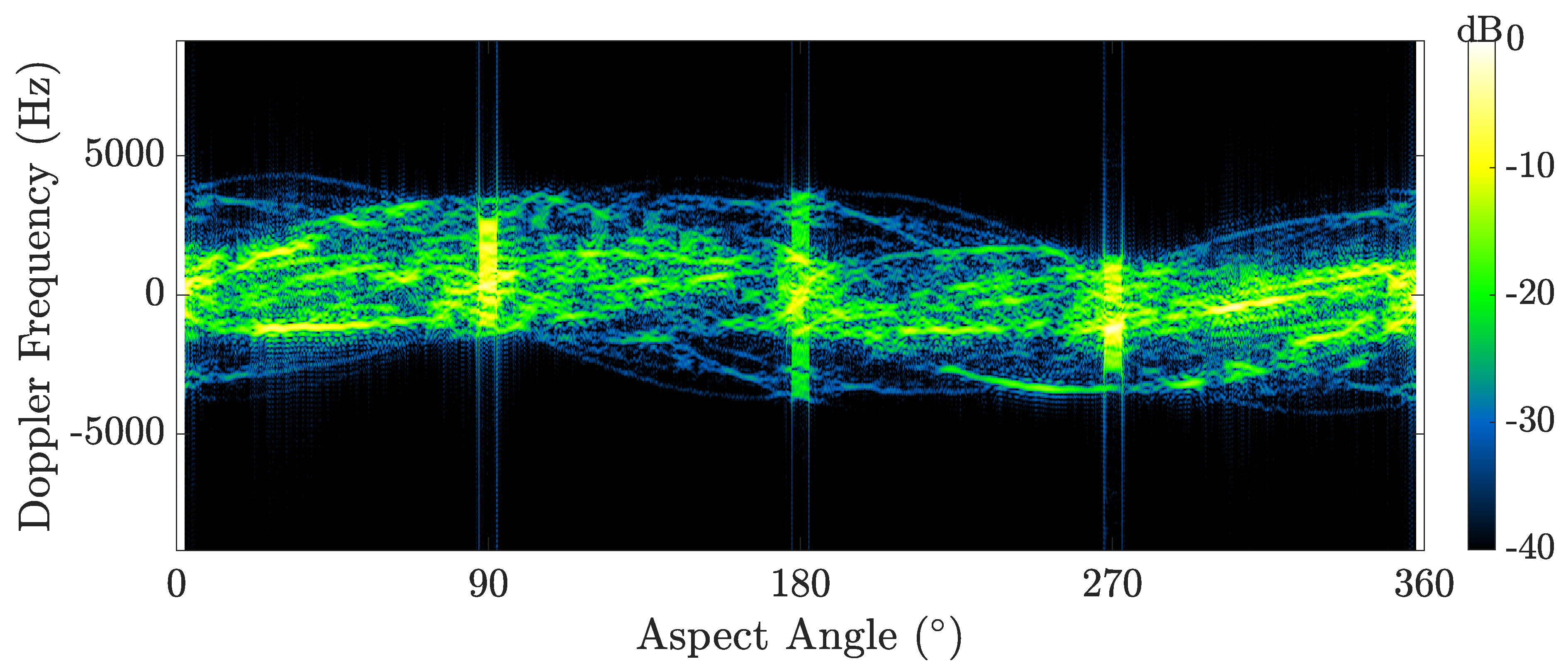
2.4.4. Doppler–Time Intensity (DTI)

Doppler–Time Intensity (DTI) plots provide snapshots of the Doppler spectrum of the object over time. The technique is ideal for cases where the object is unresolved in range but exhibits rotation relative to the radar. In these cases, the trajectories of individual scatterers are traced out over time, in a manner similar to that observed in RTI plots.

Before defining the expression for the DTI data, we first state the condition for an unresolved object in range:

$${\displaystyle |\widehat{\mathbf{u}}\left(t\right)·\mathbf{x}|<\frac{c}{2B}\mathrm{for}\mathrm{all}\mathbf{x}\in \Omega .}$$

(19)

This states that all of the scatterers are contained within a single range resolution cell. Such is often the case for narrowband radar (e.g., given 1 MHz bandwidth, the range resolution is 150 m, which is much larger than most satellites). Without loss of generality, we assume that the object return is contained within the zeroth range bin, corresponding to the point tracked by the radar. Given (19), we can express the zeroth bin of the RTI in (7) as a time series:

$${\displaystyle \widehat{g}(0,t)\approx B{\int }_{\Omega }\sigma \left(\mathbf{x}\right)exp\left({\displaystyle -j\frac{4\pi }{c}{f}_{c}R(t;\mathbf{x})}\right)d\mathbf{x}.}$$

(20)

Here, we have made use of the approximation

$$sinc\left({\displaystyle \frac{r-R(t;\mathbf{x})}{c/2B}}\right)\approx 1$$

which is valid when $|\widehat{\mathbf{u}}\left(t\right)·\mathbf{x}|\ll c/2B$.

The DTI data are computed from the time series (20) using

$$\begin{array}{cc}\hfill X_D(\dot{r},{\tau }_k)& {\displaystyle ={\int }_{{\tau }_k-T/2}^{{\tau }_k+T/2}\widehat{g}(0,t)rect\left({\displaystyle \frac{t-{\tau }_k}{T}}\right)exp\left({\displaystyle j\frac{4\pi }{c}{f}_c(t-{\tau }_k)\dot{r}}\right)dt}\hfill \\ \hfill & {\displaystyle ={\int }_{-T/2}^{T/2}\widehat{g}(0,{\overline{t}}_k+{\tau }_k)rect\left({\displaystyle \frac{{\overline{t}}_k}{T}}\right)exp\left({\displaystyle j\frac{4\pi }{c}{f}_c{\overline{t}}_k\dot{r}}\right)d{\overline{t}}_k,}\hfill \end{array}$$

(21)

where ${\overline{t}}_k=t-{\tau }_k$. This expression is equivalent to the Short-Time Fourier Transform (STFT), or spectrogram, of $\widehat{g}(0,t)$. Insertion of (20) into (21) produces

$${\displaystyle X_D(\dot{r},{\tau }_k)=BT{\int }_{\Omega }\sigma \left(\mathbf{x}\right)exp\left({\displaystyle -j\frac{4\pi }{c}{f}_{c}R({\tau }_k;\mathbf{x})}\right)sinc\left({\displaystyle \frac{\dot{r}-\dot{R}({\tau }_k;\mathbf{x})}{\lambda /2T}}\right)d\mathbf{x},}$$

(22)

where from (10)

$$\begin{array}{cc}\hfill \dot{R}({\tau }_k;\mathbf{x})& =x\dot{\theta }sin\gamma cos\left(\dot{\theta }{\tau }_k\right)-y\dot{\theta }sin\gamma sin\left(\dot{\theta }{\tau }_k\right)\hfill \\ \hfill & =\rho \dot{\theta }sin\gamma cos(\dot{\theta }{\tau }_k+\phi ),\hfill \end{array}$$

(23)

and $x=\rho cos\phi$ and $y=\rho sin\phi$. As with the range trajectory (4), the Doppler trajectory takes the form of a sinusoid, but without the height-dependent offset term. Inspection of (22) and the first equality in (23) reveals that the Doppler spectra provide projections of the target reflectivity along the cross-range axis

$$\widehat{\mathbf{q}}\left(t\right)=\left[\begin{array}{c}cos\left(\dot{\theta }t\right)sin\gamma \\ -sin\left(\dot{\theta }t\right)sin\gamma \\ 0\end{array}\right]$$

(24)

i.e., $\dot{R}({\tau }_k;\mathbf{x})=\dot{\theta }\widehat{\mathbf{q}}\left(t\right)·\mathbf{x}$. Using this fact, we will later show that the Doppler spectra can be processed using filtered backprojection techniques to form a resolved tomographic image, an approach termed Doppler tomography.

Figure 5 shows a DTI formed for a narrowband setting ($B\approx 0$ Hz) using data from the compact-range satellite model collect over a single full rotation. The bandwidth is effectively zero such that individual point scatterers are all contained within a single range bin. The DTI shows sinusoidal trajectories of different point scatterers. As observed in Figure 3, we observe bright specular flashes occur for Doppler profiles computed at aspect angle views $\theta ={90}^{\circ }\mathrm{and}{270}^{\circ }$.

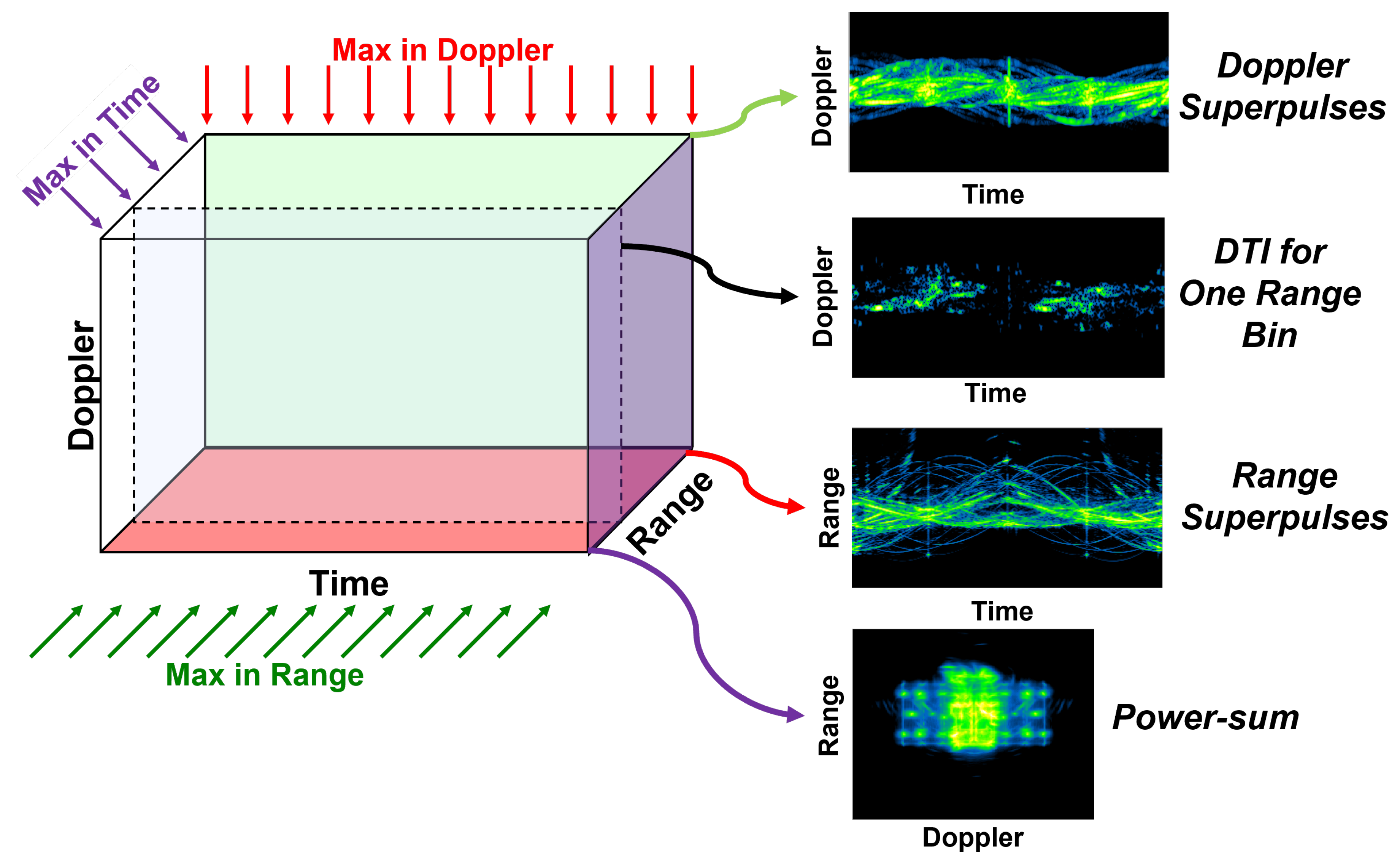
3. 3D Range-Doppler-time (RDT) Tensor Technique

In this section, we present the novel 3D RDT tensor processing technique, which provides a generalized approach to Doppler characterization, and detail the enhanced range and Doppler products that can be generated from the RDT tensor.

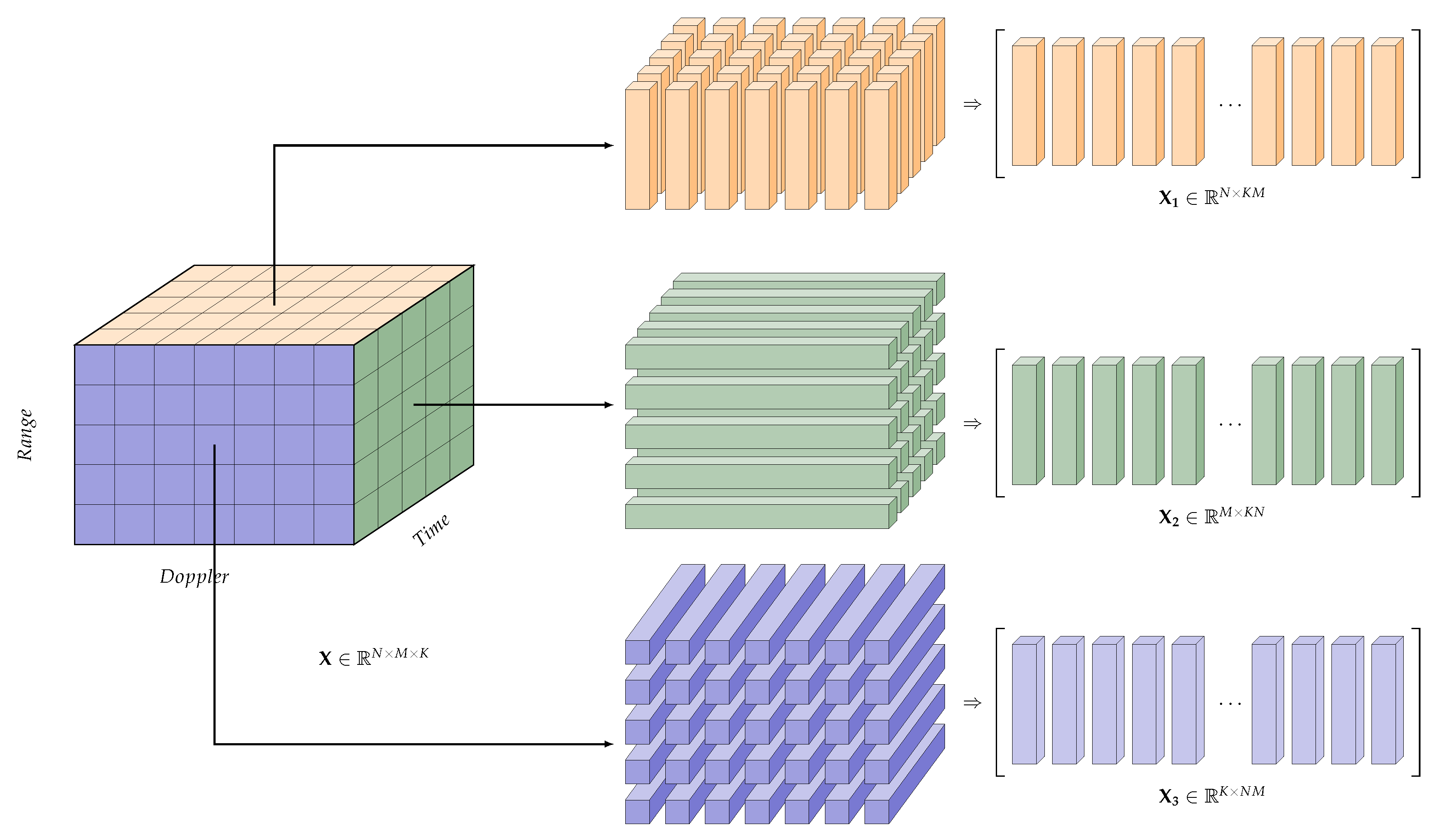
3.1. Mathematical Description

At the end of Section 2, we explored the case where the radar-signal return from a rotating object was unresolved in range, i.e., the signal was contained within a single range resolution cell. For tracking radars with wider bandwidth (greater than 10 MHz), the target may be partially resolved in range, causing it to occupy multiple range bins. Here, the DTI will not capture the complete trajectory of a scatterer when it migrates out of a range bin. To better characterize the signal in such cases, we can extend the DTI data in (21) to include a third dimension that captures the range evolution of the return:

$${\displaystyle X(r,\dot{r},{\tau }_k)={\int }_{-T/2}^{T/2}\widehat{g}(r,{\overline{t}}_k+{\tau }_k)rect\left({\displaystyle \frac{{\overline{t}}_k}{T}}\right)exp\left({\displaystyle j\frac{4\pi }{c}{f}_c{\overline{t}}_k\dot{r}}\right)d{\overline{t}}_k,}$$

(25)

where ${\overline{t}}_k=t-{\tau }_k$. We denote (25) as the range-Doppler-time (RDT) representation of the radar signal. It is convenient to express (25) as a discrete time signal to account for the fact that the radar data are sampled and processed digitally, and also to account for the inherent discrete nature of the data in slow-time arising from using a pulsed radar. This gives rise to the 3D RDT tensor

$${\displaystyle X[n,m,k]=\frac{1}{M}\sum _{l=-M/2}^{M/2-1}\widehat{g}[n,l+{\overline{l}}_k]exp\left({\displaystyle j\frac{2\pi }{M}lm}\right),}$$

(26)

where ${\overline{l}}_k=\mathrm{round}\left(f_p{\tau }_k\right)$ and $f_p$ is the pulse-repetition frequency of the radar (alternatively, one could interpolate to a grid centered about ${\tau }_k$ in place of the ‘round’ operation to achieve a more accurate result). Here, n, m, and k are range, Doppler, and time indices, respectively. Figure 6 illustrates the 3D RDT. In the next section we provide motivation for a number of useful characterization products that can be derived by collapsing (reducing) the dimensionality of the RDT, and by applying scaling/rotation transforms to the RDT. These include Doppler superpulses and range superpulses, which are enhanced versions of the DTI and RTI, respectively, and the power-sum image reconstruction, which is a non-coherent combination of RDMs across one full rotation period.

Evaluation of (26) for the object model in (5) results in

$$\begin{array}{cc}\hfill & X[n,m,k]=\hfill \\ \hfill & {\displaystyle {\int }_{\Omega }\sigma \left(\mathbf{x}\right)exp\left({\displaystyle -j\frac{4\pi }{c}{f}_{c}R({\tau }_k;\mathbf{x})}\right){\sin \mathrm{c}}_N\left({\displaystyle \frac{n{\delta }_R-R({\tau }_k;\mathbf{x})}{{\delta }_R}}\right){\sin \mathrm{c}}_M\left({\displaystyle \frac{m{\delta }_{\dot{R}}-\dot{R}({\tau }_k;\mathbf{x})}{{\delta }_{\dot{R}}}}\right)d\mathbf{x},}\hfill \end{array}$$

(27)

where ${\delta }_R=c/2B$ and ${\delta }_{\dot{R}}=\lambda /2T$ are the range and Doppler resolution cell sizes, respectively, and ${\sin \mathrm{c}}_N$ denotes a periodic sinc function of length N.

We will now examine how each scatterer in (27) evolves as a function of time. We define $\mathbf{h}({\tau }_k;\mathbf{x})$ as a 2D vector describing the position of the scatterer in range–Doppler space at each instant of time:

$$\begin{array}{cc}\hfill \mathbf{h}({\tau }_k;\mathbf{x})& =\left[\begin{array}{c}\dot{R}({\tau }_k;\mathbf{x})\\ R({\tau }_k;\mathbf{x})\end{array}\right]\hfill \\ \hfill & =\rho sin\gamma \left[\begin{array}{c}\dot{\theta }cos(\dot{\theta }{\tau }_k+\phi )\\ sin(\dot{\theta }{\tau }_k+\phi )\end{array}\right]+\left[\begin{array}{c}0\\ zcos\gamma \end{array}\right]\hfill \end{array}$$

(28)

The expression shows that each scatterer traces out a helix in a 3D range-Doppler-time space. The helix is compressed in Doppler by $\dot{\theta }$ and offset in range by the constant $zcos\gamma$.

Figure 7 shows an example RTI and RDT generated using simulated radar data for a target scene consisting of two isotropic point scatterers located at ${\mathbf{x}}_0={[4.33\mathrm{m},2.5\mathrm{m},3.0\mathrm{m}]}^T$ and ${\mathbf{x}}_1={[-2.12\mathrm{m},-2.12\mathrm{m},-2.0\mathrm{m}]}^T$, where $\gamma ={90}^{\circ }$. Here, the data were simulated at X-band ($f_c=10$ GHz) with bandwidth $B=1$ GHz. Both scatterers trace out separate helical trajectories, each described by (28). For this simulation, the rotation period of the target scene is 50 s. In Section 4.6, we highlight an example where $\gamma \ne {90}^{\circ }$, which causes the defocusing of radar-image reconstructions.

Later in this section, we will define a compressed representation of the 3D scatterer trajectory in (28) based on the pure-tumble motion assumption, and use this representation to derive a signal transform that reduces the rank of the 3D tensor in (27). The reduced-rank tensor provides a path for scatterer estimation, data denoising, and rotation-rate estimation. It also provides a framework describing the relationship between different imaging techniques.

3.2. Range and Doppler Superpulses

In radar-signal analysis, preprocessing is often applied to the RTI data in (6) to accentuate dim scatterers. One such approach is coherent presumming, which applies a boxcar filter in slow-time to coherently sum adjacent pulses. This coherent integration results in a theoretical factor of N improvement to the SNR over a single pulse for an ideal-point scatterer (constant magnitude and phase). Similarly, the generation of the RDM in (8) provides the theoretical scatterer signal-to-noise improvement. This improvement is achieved by use of the (discrete) Fourier transform, which carries out coherent integration under a variety of range-rate hypotheses (i.e., different $\dot{r}$ matched filters in (8)). A limitation of coherent presumming is that it only fully enhances scatterers with zero range rate; scatterers with non-zero range rate experience signal attenuation due to phase variation induced by the scatterer’s motion (destructive interference). This can be understood by noting that presumming returns the zero-Doppler bin of the RDM. To maximize SNR, the correct range-rate hypothesis (matched filter) must be applied when combining the pulses.

To provide a more optimal enhanced signal display, we have developed the range-superpulse concept. Here, instead of summing across a sequence of time-shifted boxcar windows, we instead generate a RDM at each window lag and return the Doppler bin with peak intensity for each range bin, thus generating a 1D signal (peak Doppler versus range). This is equivalent to collapsing the 3D RDT in Doppler using the ’max’ operation

$$X_{RS}[n,k]=\underset{m}{max}\left|X[n,m,k]\right|,$$

(29)

where $X_{RS}[n,k]$ denotes the range superpulses.

In a similar fashion, we can apply a max operation to the 3D tensor in range to generate Doppler superpulses:

$$X_{DS}[m,k]=\underset{n}{max}\left|X[n,m,k]\right|.$$

(30)

Doppler superpulses capture the energy of scatterers that migrate through multiple range resolution cells, allowing DTI techniques such as Doppler tomography to be applied to medium-band and wideband data. In [16], Doppler superpulses are found to provide superior visualizations of the imaged object in cases where the bandwidth is sufficiently large to resolve the object in range.

Figure 8 shows range superpulses generated using (29) for the compact-range dataset. Doppler superpulses for the same dataset are computed using (30) and visualized in Figure 9. Comparing and contrasting Figure 3 and Figure 8, we immediately see observed improvements in range characterization. Similarly, we observe finer Doppler characterization using superpulse processing after comparing and contrasting Figure 5 and Figure 9. Superpulse processing best serves to enhance the SNR of individual point scatterers that migrate nonlinearly across range and Doppler. These RDT-derived products enhance the sinusoidal trajectories of tumbling targets, which enables higher fidelity rotation-period estimation.

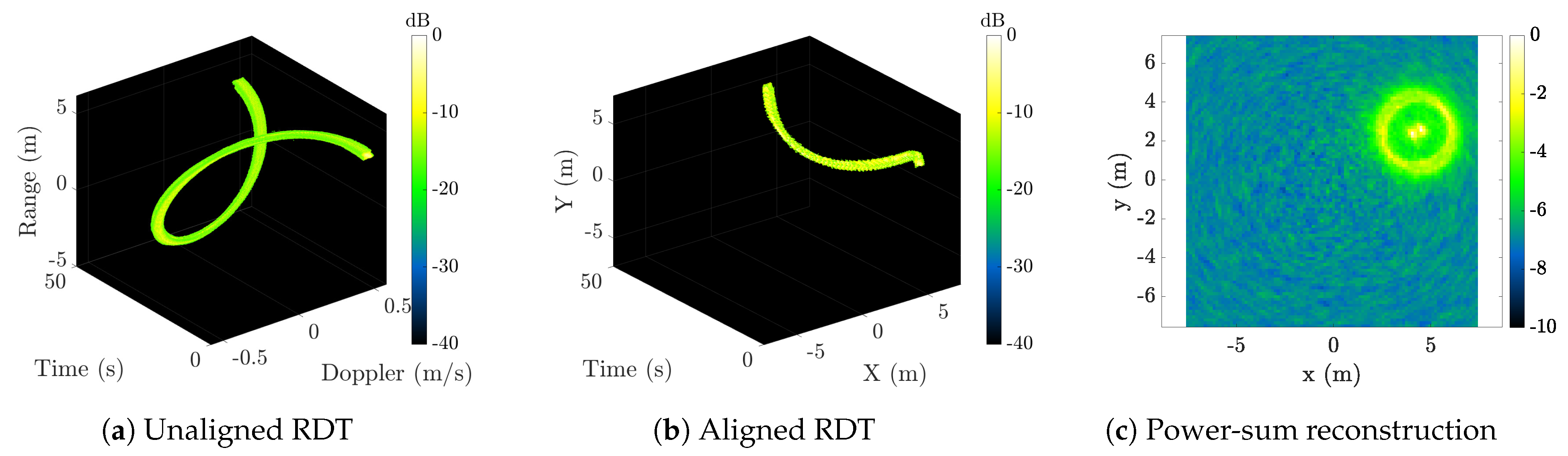
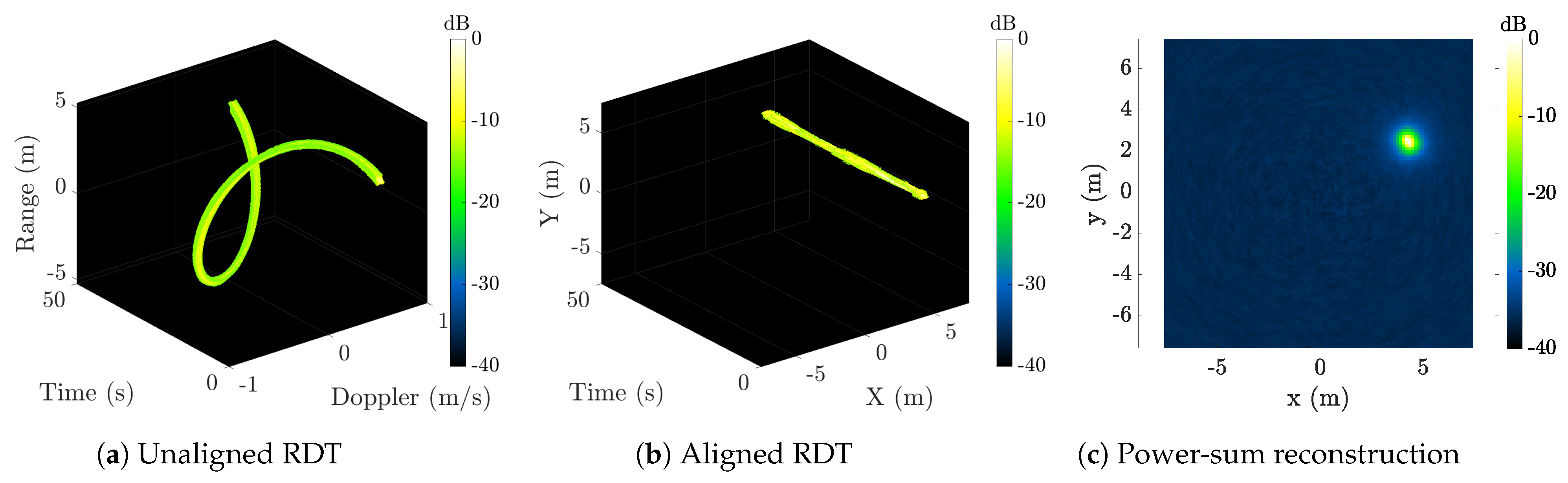
3.3. Compressed Trajectory Representation and Rank-Reducing Transform

As established by (28), each scatterer traces out a helix in a 3D tensor space. When the rotation rate $\dot{\theta }$ is known, it is possible to “unwind” the helices and map each scatterer to a spatial position. We define the transformation matrix

$${\mathbf{T}}_{\dot{\theta },\gamma }\left({\tau }_k\right)\triangleq \mathbf{R}({\tau }_k;\dot{\theta })\mathbf{diag}\left([{(\dot{\theta }sin\gamma )}^{-1},{(sin\gamma )}^{-1}]\right)$$

(31)

where $\mathbf{diag}\left(\mathbf{v}\right)$ is a diagonal matrix with $\mathbf{v}$ along the diagonal, and

$$\mathbf{R}({\tau }_k;\dot{\theta })=\left[\begin{array}{cc}cos\left(\dot{\theta }{\tau }_k\right)& sin\left(\dot{\theta }{\tau }_k\right)\\ -sin\left(\dot{\theta }{\tau }_k\right)& cos\left(\dot{\theta }{\tau }_k\right)\end{array}\right].$$

(32)

Starting with (28), we define the transformed position

$$\mathbf{p}({\tau }_k;\mathbf{x},\dot{\theta },\gamma )={\mathbf{T}}_{\dot{\theta },\gamma }\left({\tau }_k\right)\mathbf{h}({\tau }_k;\mathbf{x}).$$

(33)

This results in

$${\displaystyle \mathbf{p}({\tau }_k;\mathbf{x},\dot{\theta },\gamma )=\rho \left[\begin{array}{c}cos\phi \\ sin\phi \end{array}\right]+\frac{z}{tan\gamma }\left[\begin{array}{c}sin\left(\dot{\theta }{\tau }_k\right)\\ cos\left(\dot{\theta }{\tau }_k\right)\end{array}\right]}$$

(34)

The first term in (34) gives the x and y positions of the object in the body frame, while the second term is a depth-of-focus artifact that causes the scatterer to trace out a “donut” centered at $x,y$ with radius $z/tan\gamma$ over the rotation period. Note that when $\gamma =\pi /2$ (rotation axis orthogonal to the radar line of sight), the second term disappears, and the trajectory collapses to a single point.

We now define a signal transform that will realize the scaling and rotation operation producing the positional mapping in (34). This will be achieved by applying a geometric transformation to the continuous-time tensor data in (25). Note from (33) that

$$\mathbf{h}({\tau }_k;\mathbf{x})={\mathbf{T}}_{\dot{\theta },\gamma }^{-1}\left({\tau }_k\right)\mathbf{p}({\tau }_k;\mathbf{x},\dot{\theta },\gamma ),$$

where, by (31) and (32),

$${\mathbf{T}}_{\dot{\theta },\gamma }^{-1}\left({\tau }_k\right)=\mathbf{diag}\left([\dot{\theta }sin\gamma ,sin\gamma ]\right){\mathbf{R}}^T({\tau }_k;\dot{\theta }).$$

(35)

The continuous-time representation of the transformed RDT-tensor signal data is

$$\tilde{X}(p_y,p_x,{\tau }_k)=X\left({\mathbf{e}}_2^T{\mathbf{T}}_{\dot{\theta },\gamma }^{-1}\left({\tau }_k\right)\mathbf{p},{\mathbf{e}}_1^T{\mathbf{T}}_{\dot{\theta },\gamma }^{-1}\left({\tau }_k\right)\mathbf{p},{\tau }_k\right).$$

(36)

where $\mathbf{p}={[p_x,p_y]}^T$ and ${\mathbf{e}}_1$ and ${\mathbf{e}}_2$ are the standard basis vectors of length 2. The discrete-time counterpart of (36) is

$$\tilde{X}[n^{\prime },m^{\prime },k]=\tilde{X}\left(n^{\prime }\delta y,m^{\prime }{\delta }_x,{\tau }_k\right),$$

(37)

where ${\delta }_x$ and ${\delta }_y$ are the desired x and y pixel sizes. We refer to the matrix in (31) as the rank-reducing transform, and to the transformed tensor in (37) as the aligned RDT. In (37), the data are scaled along the range and Doppler axes to yield true position, and then rotated to a common reference frame. As a result, the helical scatterer trajectories are converted to linear ones, thus reducing the rank of the 3D tensor. If $\gamma <\pi /2$, the trajectories will exhibit some helical motion when $z\ne 0$.

Figure 10a shows an example using simulated data where the rank-reducing transform (31) has been applied to the RDT shown in Figure 7b. Note the helical trajectories of both isotropic scatterers have been rotationally aligned along the slow-time axis. Given that the imaging geometry corresponds to $\gamma ={90}^{\circ }$, the aligned trajectories described by (34) are lines. To implement (36) starting with the (discrete-time) RDT in (26), the sampled data can be interpolated to generate the desired values of the continuous-time function (25). Bilinear interpolation was used for the results in this paper.

The representation in (37) will be useful in establishing the relationship between Doppler tomography and its higher resolution counterpart BENI. As will be discussed later in the paper, the low-rank representation of the signal lends itself well to signal extraction and denoising techniques that make use of the multi-dimensional Singular Value Decomposition (SVD). In addition, (37) provides a parameterized representation of the signal that can be combined with an image-quality metric to yield an optimization-based approach for estimating the rotation rate (in cases where it is not known a priori).

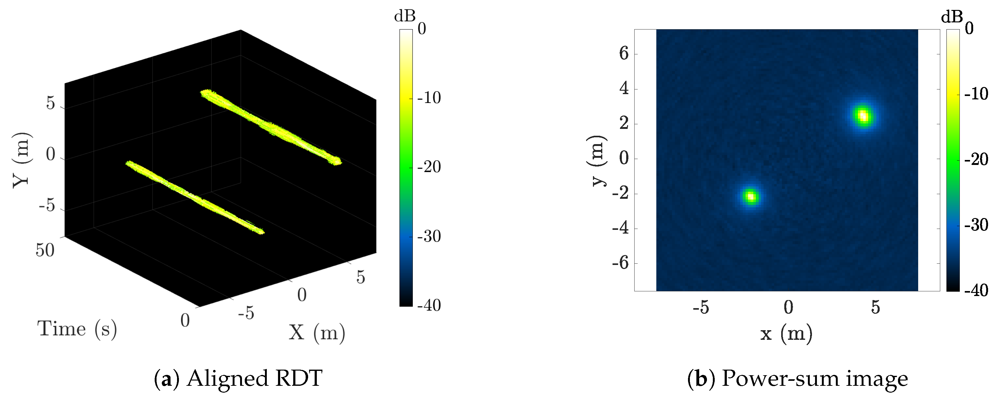
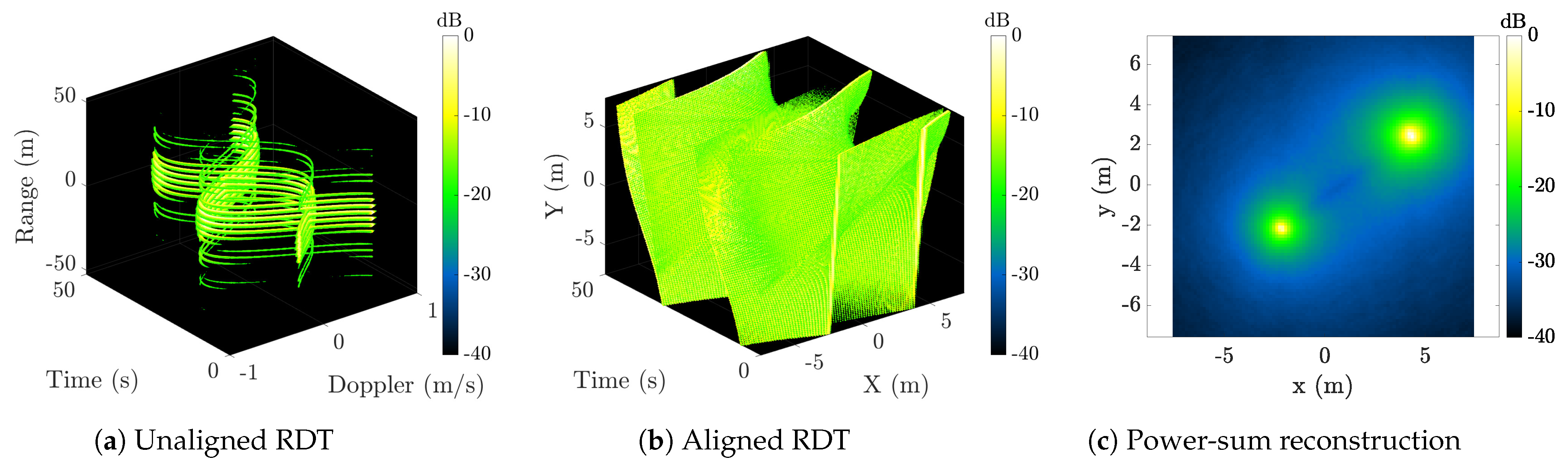
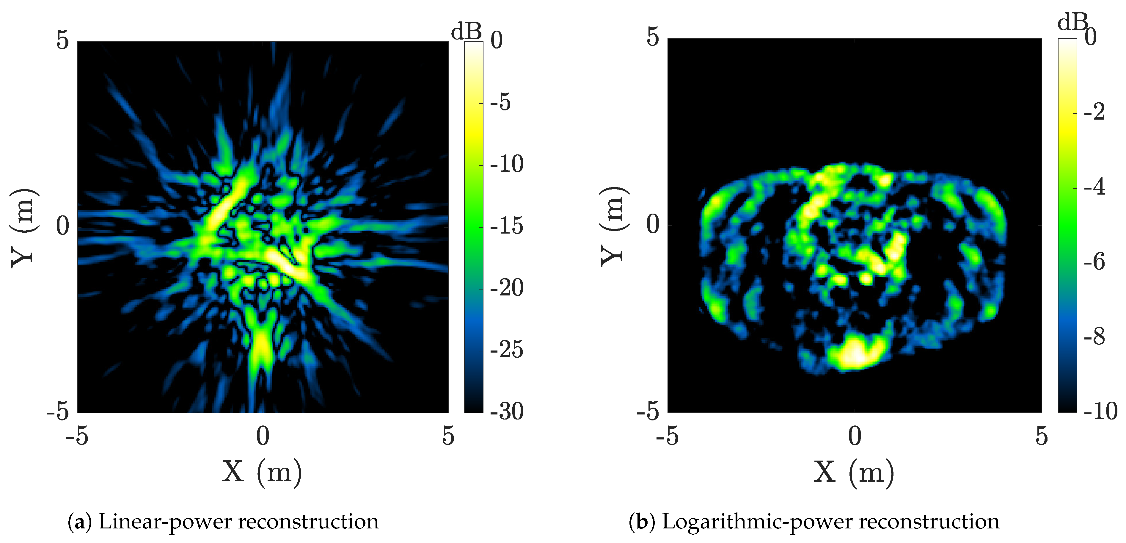
3.4. Power-Sum Image Reconstruction

In addition to superpulse processing, the RDT technique also enables radar-image reconstruction after rotational alignment using the rank-reducing transform. Consider taking the sum of the squared magnitude of the rank-reduced tensor in (37) across the time dimension. This yields

$${\displaystyle {\tilde{X}}_{PS}[n^{\prime },m^{\prime }]=\sum _{k=0}^{K-1}{\left|\tilde{X}[n^{\prime },m^{\prime },k]\right|}^2,}$$

(38)

where ${\tilde{X}}_{PS}$ denotes the power-sum image. Using (35), (36), and (37), we have

$$\begin{array}{cc}\hfill & {\tilde{X}}_{PS}[n^{\prime },m^{\prime }]=\hfill \\ \hfill & {\displaystyle \sum _{k=0}^{K-1}{\left|X\left(sin\gamma (x_{m^{\prime }}sin\left(\dot{\theta }{\tau }_k\right)+y_{n^{\prime }}cos\left(\dot{\theta }{\tau }_k\right)),\dot{\theta }sin\gamma (x_{m^{\prime }}cos\left(\dot{\theta }{\tau }_k\right)-y_{n^{\prime }}sin\left(\dot{\theta }{\tau }_k\right)),{\tau }_k\right)\right|}^2,}\hfill \end{array}$$

(39)

where $x_{m^{\prime }}={\delta }_x{m}^{\prime }$ and $y_{n^{\prime }}={\delta }_y{n}^{\prime }$.

Figure 10b shows the power-sum image derived from the aligned RDT in Figure 10a. The image accurately reproduces the two scatterers in the $x,y$ plane, which is orthogonal to the rotation axis. An example of a power-sum image generated from the compact-range data is presented in Figure 18a. As we will show in the sections that follow, the power-sum image is important to understanding the relationship between Doppler tomography and BENI, and to interpreting images from each of these techniques.

3.4.1. Relation to Doppler Tomography

Tomographic characterization of rotating objects using Doppler information, also known as Doppler tomography, is built on the principle that point scatterers along a line of constant cross-range u will reflect back radar-return signals that share the same Doppler-shifted frequency $f_D$ in traveling towards the radar [22].

We previously established that each column (i.e., fixed ${\tau }_k$) of the DTI data in (21), representing a single Doppler spectrum (or Doppler profile), provides a 1D projection of the object reflectivity along the cross-range axis in (24). Thus, the DTI data are analogous to the sinogram-domain projection data used in tomographic imaging. The Doppler tomography image is formed as

$${\displaystyle {\mathrm{g}}_{DT}(x,y)={\int }_{-T_p/2}^{T_p/2}{\left|X_D^f\left(\dot{\theta }sin\gamma (xcos\left(\dot{\theta }\tau \right)-ysin\left(\dot{\theta }\tau \right)),\tau \right)\right|}^{2}d\tau ,}$$

(40)

where

$${\displaystyle X_D^f(\dot{r},\tau )={\int }_{-T/2}^{T/2}{\widehat{X}}_D(t,\tau )\left|t\right|exp\left({\displaystyle -j\frac{4\pi }{\lambda }t\dot{r}}\right)dt}$$

is the ramp-filtered data, as required for filtered backprojection, with ${\widehat{X}}_D(t,\tau )$ denoting the inverse Fourier transform of $X_D(\dot{r},\tau )$ in Doppler [34]. Note that we apply the reconstruction to the power (squared magnitude) of the DTI data. This is due to the phase term in (22), which causes the signal to decohere when combining projections.

Doppler tomography can be viewed within the framework of the RDT technique as a special case of the power-sum reconstruction introduced in Section 3.4. Expression (39) shows how each range-Doppler slice (or RDM) of the RDT contributes to the power-sum image. In the regime where the object is unresolved in range, note that

$$\begin{array}{cc}\hfill & X\left(sin\gamma (x_{m^{\prime }}sin\left(\dot{\theta }{\tau }_k\right)+y_{n^{\prime }}cos\left(\dot{\theta }{\tau }_k\right)),\dot{\theta }sin\gamma (x_{m^{\prime }}cos\left(\dot{\theta }{\tau }_k\right)-y_{n^{\prime }}sin\left(\dot{\theta }{\tau }_k\right)),{\tau }_k\right)\hfill \\ \hfill & \approx X\left(0,\dot{\theta }sin\gamma (x_{m^{\prime }}cos\left(\dot{\theta }{\tau }_k\right)-y_{n^{\prime }}sin\left(\dot{\theta }{\tau }_k\right)),{\tau }_k\right)\hfill \end{array}$$

i.e., the signal does not vary significantly in the range dimension because the object is unresolved for all values of $x_{m^{\prime }},y_{n^{\prime }}$ over the object’s support. As a result, each column of the rank-reduced tensor is essentially an unfiltered projection, and the power-sum image is equivalent to the Doppler tomography image in (40) without the ramp-filtering step.

Figure 11 presents an example illustrating Doppler tomography as a limiting case of the power-sum reconstruction when the bandwidth is sufficiently low that the target is unresolved in range. Figure 11a shows the unaligned RDT (i.e., with no rank-reducing transform applied) for the two-scatterer example in Figure 7b, but with the bandwidth reduced from 1 GHz to 10 MHz. Here, each scatterer contributes a 1D projection to the range-Doppler slices of the RDT (note that the discretization in range is due to the range-sample spacing). Figure 11a shows the aligned RDT. The individual RDMs are rotated such that their intersection across time corresponds to the 2D scatterer position. The power-sum reconstruction is displayed in Figure 11c, revealing that both scatterers are correctly rendered.

Note over a full rotation period, the Doppler profiles of a uniformly tumbling object show signs of anisotropic scattering and are not symmetric about a half rotation. Therefore, reconstructions are computed using over $\theta \in [0,2\pi ]$.

3.4.2. Relation to Bandwidth Enhanced Non-Coherent Imaging (BENI)

BENI was designed to improve upon Doppler tomography for cases where some bandwidth is available, but the bandwidth is too small for high-resolution radar imaging. BENI has also been shown to provide exquisite detail with wideband data [28]. The first step in the algorithm is to partition radar data collected over one rotation period into a sequence of time windows of duration T centered at times ${\tau }_k$, $k=0,1,\dots K-1$, similar to DTI processing. BandWidth Extrapolation (BWE) is applied to each window to improve the range resolution [35]. The data are then resampled in range to generate equal range and cross-range pixel sizes; this step is important because the range resolution is generally much coarser than the cross-range resolution. “Local” Extended Coherent Processing (LECP) is then performed to correct linear range migration and quadratic phase error [36]; these effects arise due to deviations from the first-order approximation assumed in (9). Bandlimited interpolation is applied to the resulting images to generate a finer pixel grid. Lastly, the images are rotated to a common coordinate frame (using knowledge of $\dot{\theta }$), converted to power scale (or log-power scale), and non-coherently combined to form a single output image. The final BENI image can be represented as

$${\displaystyle {\mathrm{g}}_{BENI}(x,y)=\frac{1}{K}\sum _{k=0}^{K-1}{\left|{\mathrm{g}}_{LECP,k}\left(xcos\left(\dot{\theta }{\tau }_k\right)-ysin\left(\dot{\theta }{\tau }_k\right),xsin\left(\dot{\theta }{\tau }_k\right)+ycos\left(\dot{\theta }{\tau }_k\right)\right)\right|}^2,}$$

(41)

where ${\mathrm{g}}_{LECP,k}$ is the k-th LECP image.

Comparison of (39) and (41) reveals that the two expressions have a similar form; note that in (41), ${\mathrm{g}}_{LECP,k}$ is indexed in $x,y$ position rather than in $r,\dot{r}$, and thus, the arguments are switched. Thus, the power sum image formed from $\tilde{X}$ is essentially the BENI image, but without the BWE and motion-compensation steps. Unlike the Doppler tomography case, (41) assumes the object is partially resolved so that the signal varies along the range dimension. In other words, where the projections in Doppler tomography provide no resolving capability in range, the LECP images that BENI combines coarsely resolve the object in range, resulting in a superior reconstruction.

Using the 3D RDT tensor technique, we have established Doppler tomography as a limiting case of BENI when the bandwidth becomes sufficiently low that (19) no longer holds (the object is unresolved in range). Without BWE, BENI in this limiting case generates intermediate LECP images that have rank-1 (prior to rotational alignment). These images are essentially the same as the unfiltered backprojection images that are used for Doppler tomography.

4. Performance Assessment of RDT Tensor Processing

In this section, we analyze the RDT tensor technique in more detail, studying deviations from ideal assumptions, exploring factors that influence image quality, and highlighting challenges and edge cases associated with the imaging process.

4.1. Influence of Rotation-Rate Estimate

Successful narrowband radar imaging, where RDT-based power-sum image reconstruction is a particular approach, requires a high-fidelity rotational motion description of the space object. This section explores the influence of rotation-rate estimation errors on relative cross-range position of a single point scatterer on a uniformly rotating object. Using the target’s frame of reference, the relative cross-range position of a point scatterer is the projection of the scatterer’s position ${\mathbf{x}}_{\mathbf{p}}={[x_0,y_0,z_0]}^T$ onto the unit vector direction:

$$\begin{array}{cc}\hfill \widehat{\mathbf{q}}(t;\dot{\theta })& =\left[\begin{array}{c}cos\left(\dot{\theta }t\right)sin\gamma \\ -sin\left(\dot{\theta }t\right)sin\gamma \\ 0\end{array}\right]\hfill \end{array}$$

(42)

$$\begin{array}{cc}\hfill u({\mathbf{x}}_{\mathbf{p}},t;\dot{\theta })& =\widehat{\mathbf{q}}{\left(\mathbf{t}\right)}^T{\mathbf{x}}_{\mathbf{p}}\hfill \\ \hfill & =x_{0}cos\left(\dot{\theta }t\right)sin\gamma -y_{0}sin\left(\dot{\theta }t\right)sin\gamma .\hfill \end{array}$$

(43)

We begin our perturbation analysis by modeling an additive error in our rotation rate estimate, $ϵ$. Our updated relative cross-range measurement becomes:

$$\begin{array}{cc}\hfill u({\mathbf{x}}_{\mathbf{p}},t;\dot{\theta }+ϵ)& ={\widehat{\mathbf{q}}}^T(t;\dot{\theta }+ϵ){\mathbf{x}}_{\mathbf{p}}\hfill \\ \hfill & =x_{0}cos\left([\dot{\theta }+ϵ]t\right)sin\gamma -y_{0}sin\left([\dot{\theta }+ϵ]t\right)sin\gamma .\hfill \end{array}$$

(44)

Let $\Delta u$ denote the change in relative cross-range position resulting from inaccuracies in rotation rate estimation:

$$\begin{array}{ccc}\hfill \mathrm{(45)}& \hfill \Delta u& \triangleq u({\mathbf{x}}_{\mathbf{p}},t;\dot{\theta }+ϵ)-u({\mathbf{x}}_{\mathbf{p}},t;\dot{\theta })\hfill \hfill \mathrm{(46)}& \hfill & =x_{0}sin\gamma \left[cos\left([\dot{\theta }+ϵ]t\right)-cos\left(\dot{\theta }t\right)\right]-y_{0}sin\gamma \left[sin\left([\dot{\theta }+ϵ]t\right)-sin\left(\dot{\theta }t\right)\right]\hfill \hfill & =x_{0}sin\gamma \left[cos\left(\dot{\theta }t\right)cos\left(ϵt\right)-sin\left(\dot{\theta }t\right)sin\left(ϵt\right)-cos\left(\dot{\theta }t\right)\right]\hfill & \\ \hfill \mathrm{(47)}& \hfill & -y_{0}sin\gamma \left[sin\left(\dot{\theta }t\right)cos\left(ϵt\right)+cos\left(\dot{\theta }t\right)sin\left(ϵt\right)-sin\left(\dot{\theta }t\right)\right].\hfill \end{array}$$

Using a first-order Taylor expansion around $ϵ=0$, we simplify (47) to become the following expression:

$$\begin{array}{cc}\hfill \Delta u& \approx x_{0}sin\gamma \left[cos\left(\dot{\theta }t\right)\times 1-sin\left(\dot{\theta }t\right)\times 0-cos\left(\dot{\theta }t\right)\right]\hfill \\ \hfill & -y_{0}sin\gamma \left[sin\left(\dot{\theta }t\right)\times 1+cos\left(\dot{\theta }t\right)\times ϵt-sin\left(\dot{\theta }t\right)\right]\hfill \\ \hfill & =-y_{0}sin\gamma cos\left(\dot{\theta }t\right)ϵt.\hfill \end{array}$$

(48)

The result shown in (48) highlights cross-range position error is approximately linear both in range position as well as rotation-rate estimation error. Using (33), the 1D error (48) can be mapped to error in the 2D image plane:

$$\Delta \mathbf{p}(t;\mathbf{x},\dot{\theta })=\left[\begin{array}{c}cos\left(\dot{\theta }t\right)\\ -sin\left(\dot{\theta }t\right)\end{array}\right]y_{0}cos\left(\dot{\theta }t\right)ϵt.$$

(49)

An upper bound for the norm of the 2D error is

$$\begin{array}{cc}\hfill \parallel \Delta \mathbf{p}(t;\mathbf{x},\dot{\theta }){\parallel }_2& = |y_{0}cos\left(\dot{\theta }t\right)ϵt|\hfill \\ \hfill & \le y_0ϵT_p.\hfill \end{array}$$

(50)

If we require the 2D error to be less than one resolution cell in the power-sum image, we can derive the maximum allowable rotation-rate error. Using $d_x=d_y=\lambda /2\Delta \theta$ (i.e., the limiting narrowband case) with the requirement $\parallel \Delta \mathbf{p}(t;\mathbf{x},\dot{\theta }){\parallel }_2\le d_x$, we have the result

$${\displaystyle ϵ\le \frac{\lambda }{2\Delta \theta T_p{y}_0}.}$$

(51)

Thus, the requirement on the max rotation-rate error becomes more stringent with increasing object size (larger $y_0$), increasing rotation period $T_p$, and decreasing wavelength $\lambda$.

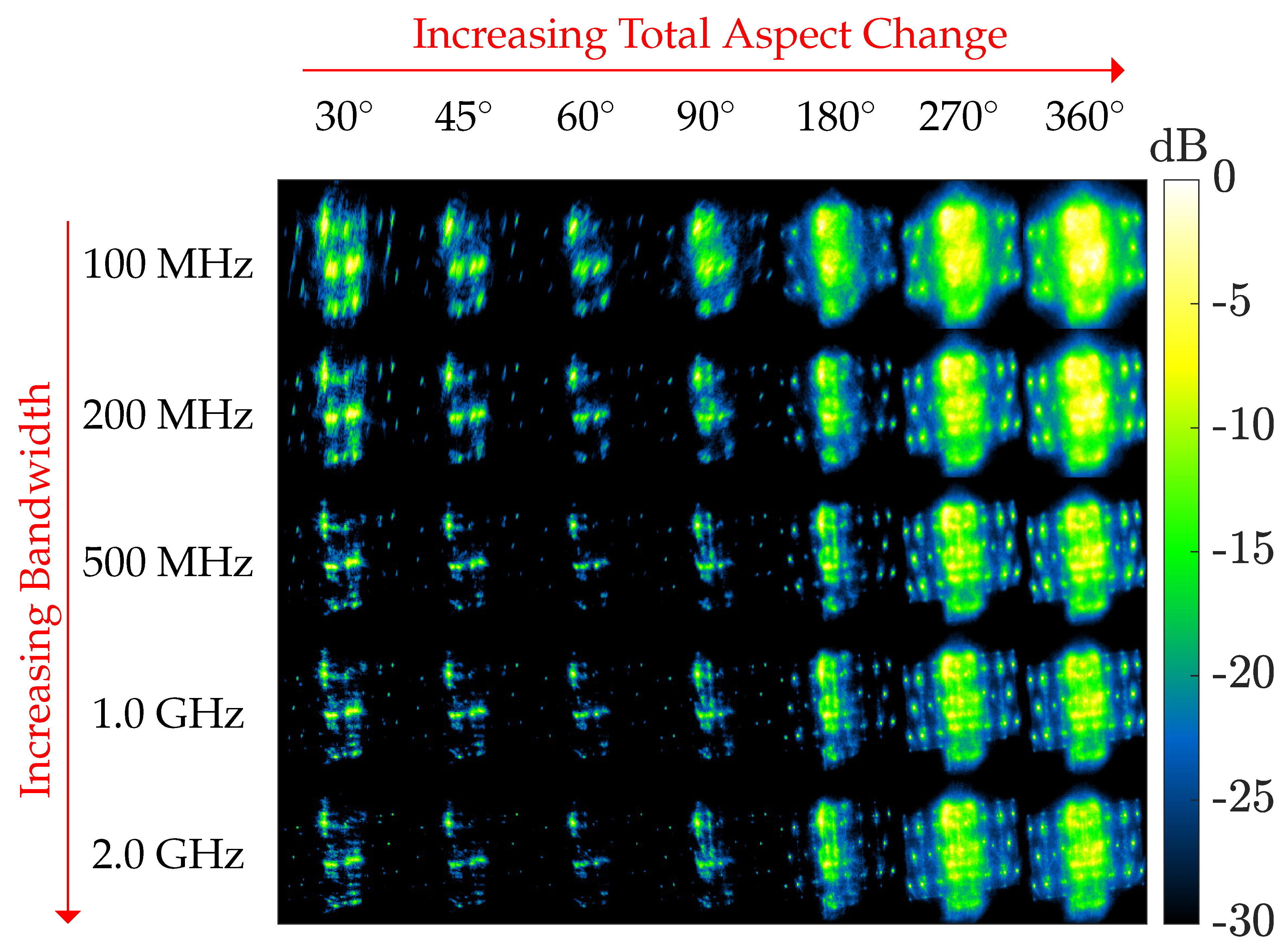
4.2. Influence of Integration Time

Selecting a suitable integration time $T_{int}$ is key to producing well-focused narrowband images. Due to the uniform rotation of the satellite, a range-dependent quadratic phase error is induced, which causes Doppler smearing of a point scatter located at $(x_p,y_p)$ on the radar-image plane. To illustrate this, we can form a second-order Taylor expansion of the phase of an individual point scatterer’s return signal around the point $(f,t)=(f_c,0)$

$$\begin{array}{cc}\hfill G_p(f,t)& \approx \underset{\mathrm{linear} \mathrm{imaging} \mathrm{approximation}}{\underbrace{exp\left[\frac{-j4\pi f{y}_p}{c}\right]exp\left[-\frac{j4\pi f_c\dot{\theta }{x}_{p}t}{c}\right]}}\hfill \\ \hfill & \times \underset{\mathrm{linear} \mathrm{range} \mathrm{walk} \mathrm{due} \mathrm{to} \mathrm{rotation}}{\underbrace{exp\left[-\frac{j4\pi (f-f_c)\dot{\theta }{x}_{p}t}{c}\right]}}\times \underset{\mathrm{quadratic} \mathrm{phase} \mathrm{error}}{\underbrace{exp\left[\frac{j2\pi f_c{\dot{\theta }}^2{y}_p{t}^2}{c}\right]}}\hfill \end{array}$$

(52)

Here, the third term generates range-walk migration. In BENI, this is corrected by applying the Keystone Transform to the data as part of LECP processing. The final term in (52) is a chirp signal. This quadratic phase expression induces smearing along cross-range. This effect worsens with increasing range $y_p$, and defocuses scatterers far away from the axis of rotation. To characterize the Doppler spread from this quadratic-motion error, we define the spectral width of the chirp term as the extent (in Doppler frequency bins) of the nearly constant magnitude response, where most of the energy of the chirp is contained. The total change in Doppler across the integration time interval can be computed as follows:

$$\begin{array}{cc}\hfill \ddot{R}& =y_p{\dot{\theta }}^2\hfill \end{array}$$

(53)

$$\begin{array}{cc}\hfill \Delta \dot{R}& =\ddot{R}\left(\frac{T_{int}}{2}\right)-\ddot{R}\left(\frac{-T_{int}}{2}\right)\hfill \\ \hfill & =y_p{\dot{\theta }}^2{T}_{int}.\hfill \end{array}$$

(54)

We define spectral width a, as the total change in Doppler divided by Doppler resolution $\delta \dot{R}=\lambda /2T_{int}$:

$$\begin{array}{cc}\hfill a& \triangleq \frac{\Delta \dot{R}}{\delta \dot{R}}\hfill \end{array}$$

(55)

$$\begin{array}{cc}\hfill & =\frac{2y_p{\dot{\theta }}^2}{\lambda }{T}_{int}^2.\hfill \end{array}$$

(56)

To ensure that the signal energies of all point scatterers are constrained within one Doppler bin (spectral width, $a\le 1$), $T_{int}$ should be selected such that:

$$\begin{array}{c}\hfill T_{int}\le \sqrt{\frac{\lambda }{2{\dot{\theta }}^2{L}_{MAX}}},\end{array}$$

(57)

where $L_{MAX}$ is defined as the object’s maximum length extent. When individual point scatterers can be resolved, acceleration error in (52) can be corrected since $y_p$ is known. This is done in BENI as part of LECP. In Doppler tomography, (57) restricts integration time per Doppler profile, which in turn influences the final image resolution.

4.3. Transient Features

Narrowband images degrade with aspect-angle-dependent scattering, as the fidelity of the rotation-rate estimation is impacted and narrowband imaging techniques such as RDT-based power-sum image reconstruction assume scatterers are present for a full rotation. For example, small targets such as cubesats are often only visible when one of their faces is perpendicular to the radar LOS. Another example of anisotropic scattering behavior is bright specular returns. This anisotropic scatterer behavior generates artifacts in the narrowband images and reduces their quality.

To overcome this problem, in Doppler tomography, filtered backprojected images are added using a logarithmic power sum (instead of a linear power sum) due to the presence of bright specular returns. Tomographic reconstructions of the compact range satellite model are shown in Figure 12. Linear-power reconstructions formed using (40) often have degraded image quality due to speculars and large sidelobes as shown in Figure 12a. Notable improvements are achieved when using logarithmic power of Doppler profiles for tomographic reconstruction. In Figure 12b, we observe structural features such as the sets of rivets on the solar panels of the satellite model.

Similarly, the final BENI image is calculated using a global logarithmic power sum of the K rotationally aligned ECP images such that

$$\begin{array}{c}\hfill g_{BENI}[x_m,y_n]=\frac{20}{K}\sum _{k=1}^K{log}_{10}\left[\left|g_k[x_m,y_n]\right|\right].\end{array}$$

(58)

We can derive a geometric-mean interpretation of the BENI reconstruction where the final image can be interpreted as a geometric average of radar cross section (RCS) over aspect-change intervals:

$$\begin{array}{cc}\hfill g_{BENI}[x_m,y_n]& =10{log}_{10}{\left[\begin{array}{c}\prod _{k=1}^K{\left|g_k[x_m,y_n]\right|}^2\end{array}\right]}^{\frac{1}{K}}\hfill \\ \hfill & =10{log}_{10}{\left[\begin{array}{c}\prod _{k=1}^K{\sigma }_{k,linear}[x_m,y_n]\end{array}\right]}^{\frac{1}{K}},\hfill \end{array}$$

(59)

where

$${\sigma }_{k,linear}[x_m,y_n]={\left|g_k[x_m,y_n]\right|}^2$$

i.e., the intensity of each pixel corresponds to RCS (for calibrated radar data). From this it can be seen that, for an isotropic point scatterer (where ${\sigma }_k$ is constant for all k), BENI image magnitude is equivalent to RCS measured in dBsm.

The expression (59) reveals why the logarithmic sum is effective in suppressing transient features. A transient feature at pixel $(x_m,y_m)$ has a magnitude near zero for at least one value of k. This results in the product of intensities also being near zero, leading to a RCS value approaching $-\infty$ dBsm in the BENI image. In contrast, a persistent scatterer contributes non-zero values for all k, thus generating a detectable feature.

4.4. Resolvability of Features

In standard radar imaging, formal definitions of resolution, which is the minimum separation at which two point scatterers can be distinguished, are well established. Typically, the peak-to-null distance of the point-spread function is used as a measure of resolution. From (18), the range and cross-range resolution of an ISAR image are ${\delta }_R=c/2B$ and ${\delta }_U=\lambda /2\Delta \theta$, respectively. We seek to establish a similar notion of resolution for power-sum imaging. To motivate this, we first examine experimental results applying BENI (a variant of power-sum imaging) to compact-range data with varying aspect change and bandwidth. We then derive analytical expressions that characterize RDT-based power-sum image resolution as a function of bandwidth, center frequency, and aspect change.

In narrowband settings, range resolution is coarse such that the target occupies a small number of range bins. Finer range resolution in BENI image reconstructions can be attributed to two processing steps. The first is Doppler-compressed BWE, which works best when the satellite consists of discrete collections of impulse-shaped features such as edges, rivets, and corner reflectors. In practice, we extrapolate by a factor of 3, $B_{eff}=3B$. For medium-band settings ($B\propto 100\mathrm{MHz}$), BWE can highlight structural features better. However, when dealing with reduced bandwidth scenarios ($B\propto 10\mathrm{MHz}$) and limited aspect-change diversity, target-scene range characterization using Doppler-compressed BWE may only offer limited improvements. The second step in BENI is globally non-coherent image reconstruction across different rotationally aligned ECP images as shown in (41). Note this image-formation step is implemented using a logarithmic power sum which has a geometric-mean interpretation as described in Section 4.3.

Figure 13 shows a matrix of examples of BENI reconstructions under varying bandwidth and aspect change. It is through exploiting wide aspect diversity that we are able to achieve better effective range resolution for drastically reduced bandwidth scenarios ($B\propto 10\mathrm{MHz}$).

In linear scale, each of the rotationally aligned images are multipled to each other in an element-wise manner prior to evaluation of the logarithm. The remainder of this section will explore the improvement in pixel resolution for a power-sum image formed using two rotationally aligned images corresponding to angle views ${\theta }_1=0^{\circ }$ and ${\theta }_2={90}^{\circ }$. This allows us to analyze two orthogonal slices through the point-spread frunction to obtain a better understanding of pixel resolution.

Figure 14 illustrates the overlapping rotationally aligned images formed over these two different angle views. Without loss of generality, we assume a point scatterer on the target is centered at the origin such that the continuous, rotationally aligned images corresponding to angle views ${\theta }_1=0^{\circ }$ and ${\theta }_2={90}^{\circ }$ have the following zero-Doppler cuts:

$$\begin{array}{cc}\hfill g_1(0,y)& =sinc\left(\frac{y}{\delta R}\right),\hfill \end{array}$$

(60)

$$\begin{array}{cc}\hfill g_2(0,y)& =sinc\left(\frac{y}{\delta \dot{R}/\dot{\theta }}\right),\hfill \end{array}$$

(61)

where $\delta R=c/2B$ and $\delta \dot{R}=c/2f_c{T}_{int}$. We will now take a closer look at the linear scale representation of the zero-Doppler cut of the corresponding power-sum image, which is the element-wise product of $0^{\circ }$ and ${90}^{\circ }$ projections as shown in Figure 14. Noting that:

$$\begin{array}{c}\hfill sinc\left(x\right)\triangleq sin\left(\pi x\right)/\pi x,\end{array}$$

(62)

$$\begin{array}{cc}\hfill g_{PS}(0,y)& =sinc\left(\frac{y}{\delta R}\right)sinc\left(\frac{y}{\delta \dot{R}/\dot{\theta }}\right)\hfill \\ \hfill & =\left(1-\frac{1}{3!}{\left[\frac{\pi y}{\delta R}\right]}^2+\frac{1}{5!}{\left[\frac{\pi y}{\delta R}\right]}^4-\cdots \right)\left(1-\frac{1}{3!}{\left[\frac{\pi y}{\delta \dot{R}/\dot{\theta }}\right]}^2+\frac{1}{5!}{\left[\frac{\pi y}{\delta \dot{R}/\dot{\theta }}\right]}^4-\cdots \right)\hfill \end{array}$$

(63)

$$\begin{array}{c}\approx 1-\frac{{\pi }^2{y}^2}{6}\left({\left[\frac{1}{\delta R}\right]}^2+{\left[\frac{1}{\delta \dot{R}/\dot{\theta }}\right]}^2\right),\hfill \end{array}$$

(64)

where (64) was obtained using a Taylor expansion of $sin\left(\pi x\right)$. Note the resulting simplified expression is a parabola and the corresponding roots of (64) provide a quantitative measure of range resolution improvement along the y-axis. The following positive root of (64) can be defined as the effective range resolution $\delta y$:

$$\begin{array}{cc}\hfill \delta y& =\frac{\sqrt{6}}{\pi }{\left({\left[\frac{1}{\delta R}\right]}^2+{\left[\frac{1}{\delta \dot{R}/\dot{\theta }}\right]}^2\right)}^{-1/2}\hfill \\ \hfill & {\displaystyle =\frac{\sqrt{6}}{\pi }\left({\displaystyle \frac{c}{2}\sqrt{{\displaystyle \frac{1}{{(f_c\Delta \theta )}^2+B^2}}}}\right).}\hfill \end{array}$$

(65)

The expression for $\delta y$ shows how both aspect change $\Delta \theta$ and bandwidth B contribute to finer characterization along the y-axis. Note that (65) can be upper bounded as

$$\begin{array}{cc}\hfill \delta y& =\frac{\sqrt{6}}{\pi }\sqrt{\frac{{\left(\delta R\right)}^2{\left(\delta \dot{R}/\dot{\theta }\right)}^2}{{\left(\delta R\right)}^2+{\left(\delta \dot{R}/\dot{\theta }\right)}^2}}\hfill \\ \hfill & <min\left\{\delta R,\delta \dot{R}/\dot{\theta }\right\}.\hfill \end{array}$$

(66)

This result demonstrates that the power-sum pixel resolution is finer than both $\delta R$ and $\delta \dot{R}/\dot{\theta }$.

4.5. Dynamic Motion: Precession and Non-Uniform Rotation

Thus far, we have assumed that the imaged object is in a pure tumble motion (uniform rotation along a fixed axis), and that the radar is stationary relative to the center of mass of the object. In practice, these assumptions do not hold perfectly, resulting in deviations from the assumed signal model. When the rotation axis varies over the collection interval, the response of a point scatterer is no longer described by the helical trajectory in (28). One important case of interest is spin-precession motion. Here, the rotation axis precesses about a fixed axis at a rate ${\dot{\theta }}_P$. The transformation from the object body frame to an inertial frame (such as ECI) can be expressed as

$${\widehat{\mathbf{u}}}_{ECI}\left(t\right)={\mathbf{U}}_P{\mathbf{R}}_z\left({\dot{\theta }}_{P}t\right){\mathbf{R}}_y\left(\beta \right){\mathbf{R}}_z\left({\dot{\theta }}_{S}t\right)\widehat{\mathbf{u}}\left(t\right),$$

(67)

where ${\mathbf{U}}_P$ is the precession coordinate frame (where the z-axis is the precession axis), $\beta$ is the angle between the precession axis and the spin axis, ${\dot{\theta }}_S$ is the spin rate, ${\dot{\theta }}_P$ is the precession rate, and $\widehat{\mathbf{u}}\left(t\right)$ and ${\widehat{\mathbf{u}}}_{ECI}\left(t\right)$ denote vectors in the body and inertial frames, respectively. The notation ${\mathbf{R}}_y\left(\beta \right)$ indicates a rotation matrix that applies a rotation of angle $\beta$ about the y axis. The application of (67) to (3) results in scatterer range and Doppler trajectories that are not purely sinusoidal, but rather, that have a time-varying amplitude modulation, phase angle, and offset. As a result, the techniques in this paper cannot be applied directly.

Another case is where the rotation axis is fixed, but the rotation rate is time varying (non-uniform rotation). If the non-uniformity can be estimated, it is possible to resample the data to equally spaced aspect angles. This enables the generation of Doppler profiles with fixed cross-range sample spacing and extent. It also allows Doppler profiles (or images) to be produced at equal angles, as desired for Doppler tomography and BENI.

Lastly, if there is relative motion between the radar and the target center of mass, as is the case for non-geostationary objects, the radar LOS is variable in the inertial frame. Thus, the model for the body-frame LOS in (1) does not hold.

The problems of estimating rotational motion parameters from the data for the cases above, and of applying these parameters to generate images, are subjects of ongoing research.

4.6. Unfavorable Imaging Geometries

As alluded to in Section 3.3, the tumble angle $\gamma$ can cause depth-of-focus effects, which degrade the quality of power-sum image reconstructions. To illustrate this, in this section we present simulated radar data modeling two wideband $(B=1\mathrm{GHz},f_c=10\mathrm{GHz})$ collects where the same single $0\mathrm{dBsm}$ peak RCS-isotropic point scatterer undergoing uniform rotation has been observed with two different geometries, where $\gamma ={90}^{\circ },\gamma ={60}^{\circ }$ for Figure 15 and Figure 16, respectively.

The rotationally aligned RDT tensor for the $\gamma ={60}^{\circ }$ scenario is displayed in Figure 16b, revealing that the isotropic point scatterer follows a residual helical trajectory. The radius of this helical path, as described by (34), is equal to $z/tan\gamma \approx 1.73\mathrm{m}$, which closely matches the radius of the circular region in Figure 16c. When $\gamma ={90}^{\circ }$, the aligned trajectory of the isotropic point scatterer is a line as shown in Figure 15b. Knowledge of $\gamma$ is needed to properly align the RDT in Figure 16a to obtain a high-fidelity power-sum image reconstruction as shown in Figure 15c.

5. Extensions to the RDT Tensor Technique

5.1. Rotational-Rate Estimation

As discussed in Section 4.1, obtaining an accurate estimate of the object’s rotation rate is critical for producing well-focused narrowband images. We aim to automate rotation-rate estimation for different target scenarios. Previous work provides a variety of techniques for estimating rotation rate, which can be split into three broad categories: time-based, frequency-based, and image quality analysis. Time-based techniques, such as auto-correlation, have been used for estimating rotational motion parameters in past work [37,38,39]. Frequency-based techniques, such as cepstrum analysis are also commonly used for identifying periodicity [40,41,42]. However, both rely on the assumption that at least one full rotation of the target object has been observed. In comparison, image-quality analysis techniques such as SIRTA, which compare image quality across a search space of possible periods, do not assume observation of more than one rotation [43,44,45].

For automating rotation-rate estimation, we are interested in more than just the ideal scenario where greater than one full rotation has been observed. In future work, we will explore different estimation techniques across a variety of scenarios with a focus on assessing the performance of the methods when only a partial rotation is observed.

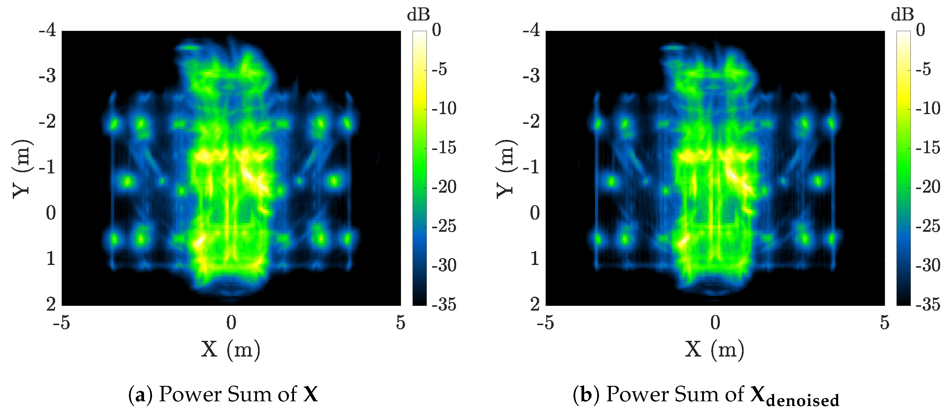
5.2. RDT Tensor Denoising Using Higher-Order Singular Value Decomposition (HOSVD)

Noting the rich three-dimensional structure of our RDT data tensor, in this section we investigate the utility of applying Higher-Order Singular Value Decomposition (HOSVD), a generalization of the matrix SVD, for image enhancement via SVD truncation [46]. After performing rotational alignment to our RDT tensor, we recognize isotropic point scatterers on an object that persist over wide-aspect diversity (such as that of a full rotation) are redundant across the slow-time dimension. This redundancy enables us to exploit low-rankness to help denoise our RDT tensor prior to reconstructing power-sum images.

The starting point of HOSVD is forming three separate matrix representations of the RDT tensor. This process is often referred to as matricization or matrix unfolding [46,47]. As visually depicted in Figure 17, we form three matricizations of the rotationally aligned RDT tensor $\mathbf{X}\in {\mathbb{R}}^{N\times M\times K}$ by rearranging mode-1 (range), mode-2 (Doppler), mode-3 (time) fibers across each dimension to form ${\mathbf{X}}_{\mathbf{1}}\in {\mathbb{R}}^{N\times KM},{\mathbf{X}}_{\mathbf{2}}\in {\mathbb{R}}^{M\times KN},{\mathbf{X}}_{\mathbf{3}}\in {\mathbb{R}}^{K\times NM}$, respectively.

For our application, we use the Tucker decomposition model for the rotationally aligned RDT tensor [47]. That is,

$$\begin{array}{cc}\hfill X[n,m,k]& =\sum _c\sum _b\sum _{a}G[a,b,c]U_1[n,a]U_2[m,b]U_3[k,c],\hfill \end{array}$$

(68)

where $\mathbf{G}\in {\mathbb{R}}^{N\times M\times K}$ is the three-dimensional core tensor consisting of singular values, and ${\mathbf{U}}_{\mathbf{1}}\in {\mathbb{R}}^{N\times N},{\mathbf{U}}_{\mathbf{2}}\in {\mathbb{R}}^{M\times M},{\mathbf{U}}_{\mathbf{3}}\in {\mathbb{R}}^{K\times K}$ are three orthonormal matrices whose columns correspond to left-singular vectors of ${\mathbf{X}}_{\mathbf{1}},{\mathbf{X}}_{\mathbf{2}},{\mathbf{X}}_{\mathbf{3}}$, respectively. ${\mathbf{U}}_{\mathbf{1}},{\mathbf{U}}_{\mathbf{2}},{\mathbf{U}}_{\mathbf{3}}$ are computed using the standard SVD whereas the core tensor $\mathbf{G}$ is computed using the Tucker’s Method 1 or HOSVD algorithm [47].

For our experiments, we computed the core tensor using the HOSVD routine in the MATLAB Tensor Toolbox [48]. We truncated singular values $G[a,b,c]$ such that we kept only nonzero values for $G[a,b,1]$, as shown in (69). This corresponds to a rank-$(N,M,1)$ approximation of $\mathbf{X}$ (rank-1 approximation along the time dimension of our tensor). We formed our denoised rotationally aligned RDT tensor using (70):

$$\begin{array}{cc}\hfill G_{truncated}[a,b,c]& =\left\{\begin{array}{cc}G[a,b,c]\hfill & \mathrm{if}c=1\hfill \\ 0\hfill & \mathrm{if}c\ne 1\hfill \end{array}\right.\hfill \end{array}$$

(69)

$$\begin{array}{cc}\hfill X_{denoised}[n,m,k]& =\sum _c\sum _b\sum _a{G}_{truncated}[a,b,c]U_1[n,a]U_2[m,b]U_3[k,c]\hfill \\ \hfill & =U_3[k,1]\sum _b\sum _{a}G[a,b,1]U_1[n,a]U_2[m,b].\hfill \end{array}$$

(70)

Figure 18 compares and contrasts the full rank-($N,M,K)$ logarithmic power-sum image reconstructions to that of the reduced rank-$(N,M,1)$ logarithmic power-sum image reconstruction. Note the sharper appearance of rivets and edges on the solar panels of the compact-range satellite. Future work involves a continued investigation into tensor decompositions for radar-image enhancement.

6. Conclusions

In this work, we proposed a powerful unified technique for narrowband radar deep-space satellite characterization. Using our three-dimensional RDT tensor representation of radar signals, we generated RDT-derived products such as range superpulses, Doppler superpulses, and power-sum image reconstructions. Utilizing radar data obtained for a compact-range satellite model, we demonstrated that each of these RDT-derived products successfully enhanced range and Doppler characterization. We also established the equivalence of BENI and Doppler tomography narrowband imaging techniques as different versions of power-sum reconstructions using the rank-reduced RDT. In addition, we quantified limitations of these radar imaging techniques as a function of carrier frequency, sensitivity, integration time, and rotation-rate estimate uncertainty. Another accomplished objective of this work included providing interpretability of RDT-based power-sum images with respect to pixel RCS measurements over varying imaging geometries (orientations of the object). For future work, we will continue to address challenges encountered when deviating from ideal radar-signal models, and explore other ways to exploit the rich RDT data structure for radar-image enhancement.

References

1. Sridharan, R.; Pensa, A. Perspectives in Space Surveillance; MIT Press: Cambridge, MA, USA, 2017. [Google Scholar]
2. Walker, J. Range-Doppler imaging of rotating objects. IEEE Trans. Aerosp. Electron. Syst. 1980, AES-16, 23–52. [Google Scholar] [CrossRef]
3. Munson, D.; O’Brien, D.; Jenkins, W. A tomographic formulation of spotlight-mode synthetic aperture radar. Proc. IEEE 1983, 71, 917–925. [Google Scholar] [CrossRef]
4. Swenson, A.T.; Nebelecky, C.K.; Wilkinson, D.; Crassidis, J.L. Resident Space Object Shape and Material Estimation using Polarimetric Data. In Proceedings of the AAS Guidance, Navigation and Control (GN&C Conference), Sopot, Poland, 12–16 June 2023; pp. 23–140. [Google Scholar]
5. Dianetti, A.; Crassidis, J. Resident Space Object Characterization Using Polarized Light Curves. J. Guid. Control Dyn. 2022, 46, 1–18. [Google Scholar] [CrossRef]
6. Anderson, J.D.; Anderson, A.J.; Zuehlke, D.A.; Canales, D.; Lovell, T.A. Resident Space Object Identification in Arbitrary Unresolved Space Images. In Proceedings of the Proceedings of the 33rd AAS/AIAA Space Flight Mechanics Meeting], AAS/AIAA, Austin, TX, USA, 15–19 January 2023. [Google Scholar]
7. Suthakar, V.; Sanvido, A.A.; Qashoa, R.; Lee, R.S.K. Comparative Analysis of Resident Space Object (RSO) Detection Methods. Sensors 2023, 23, 9668. [Google Scholar] [CrossRef] [PubMed]
8. Wu, X.; Sahoo, D.; Hoi, S.C. Recent advances in deep learning for object detection. Neurocomputing 2020, 396, 39–64. [Google Scholar] [CrossRef]
9. Massimi, F.; Ferrara, P.; Benedetto, F. Deep Learning Methods for Space Situational Awareness in Mega-Constellations Satellite-Based Internet of Things Networks. Sensors 2023, 23, 124. [Google Scholar] [CrossRef]
10. Linares, R.; Furfaro, R. Space Object classification using deep Convolutional Neural Networks. In Proceedings of the 2016 19th International Conference on Information Fusion (FUSION), Heidelberg, Germany, 5–8 July 2016; pp. 1140–1146. [Google Scholar]
11. Jia, B.; Pham, K.; Blasch, E.; Wang, Z.; Shen, D.; Chen, G. Space object classification using deep neural networks. In Proceedings of the 2018 IEEE Aerospace Conference, Big Sky, MT, USA, 3–10 March 2018; pp. 1–8. [Google Scholar] [CrossRef]
12. Linares, R.; Furfaro, R.; Reddy, V. Space Objects Classification via Light-Curve Measurements Using Deep Convolutional Neural Networks. J. Astronaut. Sci. 2020, 67, 1063–1091. [Google Scholar] [CrossRef]
13. Qashoa, R.; Lee, R. Classification of Low Earth Orbit (LEO) Resident Space Objects’ (RSO) Light Curves Using a Support Vector Machine (SVM) and Long Short-Term Memory (LSTM). Sensors 2023, 23, 6539. [Google Scholar] [CrossRef] [PubMed]
14. Furfaro, R.; Linares, R.; Gaylor, D.; Jah, M.; Walls, R. Resident space object characterization and behavior understanding via machine learning and ontology-based bayesian networks. In Proceedings of the Advanced Maui Optical and Space Surveillance Technologies Conference, Maui, HI, USA, 20–23 September 2016; p. 35. [Google Scholar]
15. AlDahoul, N.; Karim, H.A.; De Castro, A.; Tan, M.J.T. Localization and classification of space objects using EfficientDet detector for space situational awareness. Sci. Rep. 2022, 12, 21896. [Google Scholar] [CrossRef]
16. Serrano, A.; Morrison, R.L. Doppler Superpulse Processing for Improved Tomographic Characterization of Space Objects. In Proceedings of the 2023 IEEE International Applied Computational Electromagnetics Society Symposium (ACES), Monterey, CA, USA, 26–30 March 2023; pp. 1–2. [Google Scholar]
17. Chua, C. Doppler-Only Synthetic Aperture Radar. Master’s Thesis, Naval Postgraduate School, Monterey, CA, USA, 2006. [Google Scholar]
18. Androsov, A.; Vygon, V.; Ustinov, N. Reconstruction of images of rotating bodies of arbitrary angular dimensions. I. Structure of Doppler spectra and reconstruction of images from projections. Sov. J. Quantum Electron. 1985, 15, 168–172. [Google Scholar] [CrossRef]
19. Marino, R.; Capes, R.; Keicher, W.; Kulkarni, S.; Parker, J.; Swezey, L. Tomographic image reconstruction from laser radar reflective projections. In Proceedings of the Proc. SPIE 0999; Laser Radar III; SPIE: Bellingham, WA, USA, 1989; pp. 248–268. [Google Scholar]
20. Chen, V. Analysis of radar micro-Doppler with time-frequency transform. In Proceedings of the Tenth IEEE Workshop on Statistical Signal and Array Processing, Pocono Manor, PA, USA, 16 August 2000; pp. 463–466. [Google Scholar]
21. Coetzee, S.; Baker, C.; Griffiths, H. Narrow band high resolution radar imaging. In Proceedings of the 2006 IEEE Conference on Radar, Verona, NY, USA, 24–27 April 2006; pp. 622–625. [Google Scholar]
22. Mensa, D.L.; Halevy, S.; Wade, G. Coherent Doppler tomography for microwave imaging. Proc. IEEE 1983, 71, 254. [Google Scholar] [CrossRef]
23. Das, Y.; Boerner, W. On radar target shape estimation using algorithms for reconstruction from projections. IEEE Trans. Antennas Propag. 1978, AP-26, 274–279. [Google Scholar] [CrossRef]
24. Bai, X.; Sun, G.; Wu, Q.; Xing, M.; Bao, Z. Narrow-band radar imaging of spinning targets. Sci. China Inf. Sci. 2011, 54, 873–883. [Google Scholar] [CrossRef]
25. Lanterman, A.; Munson, D.; Wu, Y. Wide-angle radar imaging using time–frequency distributions. IEE Proc.-Radar Sonar Navig. 2003, 150, 203–211. [Google Scholar] [CrossRef]
26. Sun, H.; Feng, H.; Lu, Y. High resolution radar tomographic imaging using single-tone CW signals. In Proceedings of the 2010 IEEE Conference on Radar, Lecce, Italy, 21–25 June 2010; pp. 975–980. [Google Scholar]
27. McCoy, J.; Magotra, N.; Chang, B. Coherent Doppler tomography—A technique for narrow band SAR. IEEE Aerosp. Electron. Syst. Mag. 1991, 6, 19–22. [Google Scholar] [CrossRef] [PubMed]
28. Serrano, A.; Morrison, R.L. BENI: Bandwidth Enhanced Noncoherent Imaging of Rotating Objects. In Proceedings of the 2022 IEEE Radar Conference (RadarConf22), New York, NY, USA, 21–25 March 2022; pp. 1–6. [Google Scholar] [CrossRef]
29. Serrano, A.; Kobsa, A.; Uysal, F.; Cerutti-Maori, D.; Ghio, S.; Kintz, A.; Morrison, R.L., Jr.; Welch, S.; van Dorp, P.; Hogan, G.; et al. Long baseline bistatic radar imaging of tumbling space objects for enhancing space domain awareness. IET Radar Sonar Navig. 2023. [Google Scholar] [CrossRef]
30. Uysal, F.; Dorp, P.v.; Serrano, A.; Kobsa, A.; Ghio, S.; Kintz, A.; Bassa, C.; Garrington, S.; Cuenca, M.C.; Otten, M.; et al. Large Baseline Bistatic Radar Imaging for Space Domain Awareness. In Proceedings of the 2023 IEEE International Radar Conference (RADAR), Sydney, Australia, 6–10 November 2023; pp. 1–6. [Google Scholar] [CrossRef]
31. Benson, C.J.; Naudet, C.J.; Lowe, S.T. Radar Study of Inactive Geosynchronous Earth Orbit Satellite Spin States. Interplanet. Prog. Rep. 2020, 42, 1–14. [Google Scholar]
32. Coulombe, M.J.; Horgan, T.; Waldman, J.; Neilson, J.; Carter, S.; Nixon, W. A 160 GHz Polarimetric Compact Range for Scale Model RCS Measurements. In Proceedings of the Antenna Measurements and Techniques Association (AMTA), Seattle, WA, USA, 30 September–3 October 1996; p. 239. [Google Scholar]
33. High Fidelity Satellite Model in STL Radar Range. Available online: https://www.uml.edu/research/stl/ (accessed on 30 September 2023).
34. Kak, A.; Slaney, M. Principles of Computerized Tomographic Imaging; IEEE Press: New York, NY, USA, 1988. [Google Scholar]
35. Borison, S.; Bowling, S.; Cuomo, K. Super-resolution methods for wideband radar. Linc. Lab. J. 1992, 5, 441–461. [Google Scholar]
36. Ausherman, D.; Kozma, A.; Walker, J.; Jones, H.; Poggio, E. Developments in radar imaging. IEEE Trans. Aerosp. Electron. Syst. 1984, AES-16, 363–398. [Google Scholar] [CrossRef]
37. Xing, Y.; You, P.; Yong, S. Parameter Estimation of Micro-Motion Targets for High-Resolution-Range Radar Using Online Measured Reference. Sensors 2018, 18, 2773. [Google Scholar] [CrossRef]
38. Yang, Q.; Deng, B.; Wang, H.; Qin, Y. Parameter Estimation and Image Reconstruction of Rotating Targets with Vibrating Interference in the Terahertz Band. J. Infrared Millim. Terahertz Waves 2017, 38, 909–928. [Google Scholar] [CrossRef]
39. Zhang, W.; Li, K.; Jiang, W. Parameter Estimation of Radar Targets with Macro-Motion and Micro-Motion Based on Circular Correlation Coefficients. IEEE Signal Process. Lett. 2015, 22, 633–637. [Google Scholar] [CrossRef]
40. Bogert, B.P.; Healy, M.J.; Tukey, J.W. The quefrency analysis of time series for echoes: Cepstrum, pseudo-autocovariance, cross-cepstrum and saphe cracking. In Proceedings of the Symposium on Time Series Analysis, Providence, RI, USA, 11–14 June 1963. [Google Scholar]
41. Oppenheim, A.; Schafer, R. From frequency to quefrency: A history of the cepstrum. IEEE Signal Process. Mag. 2004, 21, 95–106. [Google Scholar] [CrossRef]
42. Lee, J.K.; Kabrisky, M.; Oxley, M.E.; Rogers, S.K.; Ruck, D.W. The complex cepstrum applied to two-dimensional images. Pattern Recognit. 1993, 26, 1579–1592. [Google Scholar] [CrossRef]
43. Ghio, S.; Martorella, M. Estimation of Rotating RSO Parameters using Radar Data and Joint Time-Frequency Transforms. In Proceedings of the 7th Eur Conf. Space Debris, Darmstadt, Germany, 18–21 April 2017. [Google Scholar]
44. Ghio, S.; Martorella, M.; Staglianò, D.; Petri, D.; Lischi, S.; Massini, R. Practical implementation of the spectrogram-inverse Radon transform based algorithm for resident space objects parameter estimation. IET Sci. Meas. Technol. 2019, 13, 1254–1259. [Google Scholar] [CrossRef]
45. Ghio, S.; Martorella, M.; Staglianò, D.; Petri, D.; Lischi, S.; Massini, R. Experimental Comparison of Radon Domain Approaches for Resident Space Object’s Parameter Estimation. Sensors 2021, 21, 1298. [Google Scholar] [CrossRef] [PubMed]
46. De Lathauwer, L.; De Moor, B.; Vandewalle, J. A Multilinear Singular Value Decomposition. SIAM J. Matrix Anal. Appl. 2000, 21, 1253–1278. [Google Scholar] [CrossRef]
47. Kolda, T.G.; Bader, B.W. Tensor Decompositions and Applications. SIAM Rev. 2009, 51, 455–500. [Google Scholar] [CrossRef]
48. Kolda, T.G.; Bader, B.W.; Acar Ataman, E.N.; Dunlavy, D.; Bassett, R.; Battaglino, C.J.; Plantenga, T.; Chi, E.; Hansen, S. Tensor Toolbox for MATLAB v. 3.5; MathWorks Company: Portola Valley, CA, USA, 2023. [Google Scholar]
Figure 1. Turntable imaging with the target’s center of mass at the origin.
Remotesensing 16 01374 g001
Figure 2. Uniformly rotating compact-range satellite model [33].
Remotesensing 16 01374 g002
Figure 3. RTI for compact-range satellite model observed over a full rotation.
Remotesensing 16 01374 g003
Figure 4. (a) Range–Doppler Map and (b) ISAR image reconstructions of the compact-range satellite model.
Remotesensing 16 01374 g004
Figure 5. DTI for the compact-range satellite model observed over a full rotation.
Remotesensing 16 01374 g005
Figure 6. 3D RDT tensor.
Remotesensing 16 01374 g006
Figure 7. Simulated (a) RTI and (b) RDT for a target scene.
Remotesensing 16 01374 g007
Figure 8. Range superpulses, X R S [ n , k ] , for the compact-range satellite model observed over a full rotation.
Remotesensing 16 01374 g008
Figure 9. Doppler superpulses, X D S [ m , k ] , for the compact-range satellite model observed over a full rotation.
Remotesensing 16 01374 g009
Figure 10. (a) Rotationally aligned RDT for target scene in Figure 7, and (b) corresponding power-sum image.
Remotesensing 16 01374 g010
Figure 11. Imaging example for the two-scatterer geometry in Figure 7b, but using a narrowband waveform with 10 MHz bandwidth.
Remotesensing 16 01374 g011
Figure 12. Doppler tomography reconstructions formed using (a) linear power and (b) logarithmic power of Doppler profiles of the rotating compact-range satellite model.
Remotesensing 16 01374 g012
Figure 13. Limited aspect change and reduced bandwidth BENI reconstructions of the compact-range satellite model.
Remotesensing 16 01374 g013
Figure 14. Power-sum reconstruction pixel resolution illustration.
Remotesensing 16 01374 g014
Figure 15. Simulated imaging geometry of uniformly rotating point scatterer where γ = 90 .
Remotesensing 16 01374 g015
Figure 16. Simulated imaging geometry of uniformly rotating point scatterer where γ = 60 .
Remotesensing 16 01374 g016
Figure 17. Matricization of the RDT Tensor.
Remotesensing 16 01374 g017
Figure 18. Logarithmic power-sum image reconstructions formed using (a) full-rank approximation X and (b) HOSVD truncation to form rank- ( N , M , 1 ) approximation of X .
Remotesensing 16 01374 g018
Disclaimer/Publisher’s Note: The statements, opinions and data contained in all publications are solely those of the individual author(s) and contributor(s) and not of MDPI and/or the editor(s). MDPI and/or the editor(s) disclaim responsibility for any injury to people or property resulting from any ideas, methods, instructions or products referred to in the content.