Abstract
Spartina alterniflora (S. alterniflora) has grown rapidly in China since its introduction in 1979, showing the trend of alien species invasion, which has seriously affected the ecosystem balance of coastal wetlands. The temporal and spatial expansion law of S. alterniflora can be obtained through remote sensing monitoring, which can provide a reference and basis for S. alterniflora management. This paper presents a method for extracting and mapping S. alterniflora based on phenological characteristics. The coastal areas of the Yangtze River Delta Urban Agglomeration are selected as the research area, and the Landsat time series data from 1990 to 2022 on the Google Earth Engine (GEE) platform are used to support the experiment in this paper. Firstly, the possible growing area of S. alterniflora was extracted using the normalized differential moisture index (NDMI), normalized differential vegetation index (NDVI), and normalized differential water index (NDWI); Then, the time series curve characterizing the phenological characteristics of vegetation was constructed using the vegetation index to determine the difference phase of phenological characteristics between S. alterniflora and other vegetation. Finally, a decision tree was constructed based on the phenological feature difference phase data to extract S. alterniflora, and it is applied to the analysis of temporal and spatial changes of S. alterniflora in the study area from 1990 to 2022. The results show that the area of S. alterniflora increased from ~1426 ha in 1990 to ~44,508 ha in 2022. However, the area of S. alterniflora began to show negative growth in 2015 due to the construction of nature reserves and ecological management. The results of correlation analysis showed that the growth of C. japonicum was significantly affected by temperature stress and weakly affected by precipitation. This study verified that Landsat time series images can effectively extract vegetation phenological information, which has strong feasibility for extraction and dynamic monitoring of S. alterniflora and provides technical support for the management and monitoring of invasive plants in coastal wetlands.
1. Introduction
S. alterniflora is one of the main vegetation types introduced to coastal areas, which is mainly used to protect the beaches and coasts of China’s coastal zones from erosion and damage from waves and has certain economic value [1,2,3,4,5,6,7]. Due to its adaptability to salt and flooding, it usually grows densely on the high-salinity tidal flats in the intertidal zone, meaning it occupies the growth space of mangroves, changing the physical and chemical properties of the soil, altering biodiversity and behavior patterns, affecting the species composition and community structure of benthic animals, etc., leading to the disappearance of large mangroves [8,9,10,11,12,13].
The invasion of S. alterniflora has occurred since its introduction to China in 1979, which has caused great impacts on the coastal wetland ecosystem [14,15,16,17]. At present, it is widely distributed in the tidal flats from Tianjin to Guangxi. In the Yellow River Delta, Chongming Dongtan, Yancheng Wetland, and other important coastal wetlands, the invasion trend is irreversible [4,18]. Accurate monitoring of S. alterniflora growth dynamic information can provide guidance and a basis for the sustainable development of coastal wetlands, and provide multi-level, multi-temporal information and technical support for the research and management of coastal wetlands [19,20].
Remote sensing technology data have the characteristics of being multi-source, practical and economical, real-time and efficient, and having repeatable monitoring, etc., and have gradually become the main means of dynamic monitoring of coastal wetlands [21,22,23,24,25]. The current research methods mainly include three types. One is the extraction of S. alterniflora based on single-temporal remote sensing images. The traditional methods are to visually interpret single or multiple images to generate the spatial distribution dataset of S. alterniflora [26,27]. These methods are labor-intensive and time-consuming. Due to differences in the experience of researchers, the results of visual interpretation will vary greatly [28]. Based on high-resolution images such as Google Earth, SPOT5, and GF-1, Liu used visual interpretation and object-oriented methods to obtain the area distribution of S. alterniflora in the Zhangjiang wetlands, Fujian Province from 2003 to 2015 [29]. However, visual interpretation can only identify coastal wetland vegetation of a single type and with a significant difference in spectral characteristics, which has high cost and limited classification accuracy via human interpretation. The second is the extraction of S. alterniflora based on multi-source and multi-temporal remote sensing images. Some scholars also use multi-temporal hyperspectral and multispectral images to calculate spatial features, vegetation index and image texture information, and apply supervised or unsupervised classification algorithms to obtain the distribution map of S. alterniflora [30,31]. Li et al. used Landsat TM/OLI time series images to draw the distribution map of the flowering plants in Zhejiang Province from 1985 to 2015 based on the expert knowledge threshold method [32]. Wang et al. used Landsat and Spot-6 images to analyze the growth rate and pattern of S. alterniflora in Yueqing Bay from 1993 to 2014 based on support vector machine and object-oriented analysis methods [33]. However, only relying on the object-oriented classification method to extract vegetation information will be strongly interfered with by the vegetation spectrum, and the extraction accuracy needs to be improved. Moreover, due to the lack of data and image quality problems, it is impossible to realize large-scale and long-time dynamic monitoring. The third is the extraction of S. alterniflora based on multi-temporal images and phenological characteristics. In recent years, the algorithm based on pixel and phenology has been applied in many fields such as crops, forest planting, coastal beach, and coastal vegetation. Tian proposed a spectral phenological characterization method of S. alterniflora, which synthesized the growth period of S. alterniflora into two phenological stages and classified them using the support vector machine classifier [34]. Through field investigations, Zhang found that the NDVI of the senescence stage is considered to be an effective datum to identify S. alterniflora salt marshes [35]. Sun proposed a salt marsh vegetation classification method based on the phenological parameters of Sentinel-2 pixel differential time series (PDTS), and used the random forest algorithm for plant species classification [36]. However, the potential of long time series Landsat images in tracking phenological differences between S. alterniflora and other salt marsh vegetation has not been fully evaluated.
Although remote sensing technology has been widely used in wetland vegetation monitoring, the existing remote sensing monitoring research is still insufficient due to the complexity of coastal wetland ecosystems. This is mainly reflected in that S. alterniflora has the same spectrum as other vegetation, which is difficult to distinguish effectively using only one scene image. The machine learning classification method considering phenological characteristics highly depends on the sample quality, so it is necessary to comprehensively consider the relationship between vegetation and geographical habitat factors in the classification method. Based on this, this paper proposes an extraction method of S. alterniflora based on Collaborative Geoscience Knowledge and vegetation phenological feature decision. The purpose of this study is as follows: (1) to obtain a method of extracting S. alterniflora based on phenological feature decision; (2) to analyze the temporal and spatial evolution characteristics of S. alterniflora in the Yangtze River Delta in the most recent 30 years; (3) to explore the phenological differences of S. alterniflora at different latitudes.
2. Materials
2.1. Study Area
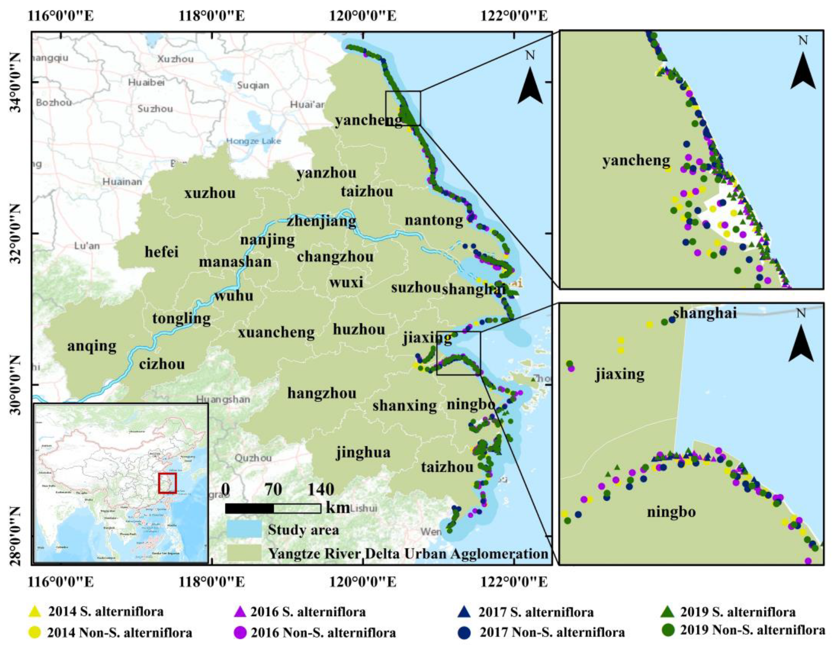
The Yangtze River Delta Urban Agglomeration (32°34′N–29°20′N, 115°46′E–123°25′E) is located in the middle and lower reaches of the Yangtze River Plain (Figure 1), adjacent to the Yellow Sea and the East China Sea, with a total administrative area of 212,500 km2. The Yangtze River Delta urban agglomeration is located in the subtropical monsoon climate, the annual average temperature is about 15.7 °C, and the annual precipitation is about 1158 mm. The Yangtze River Delta is the area with the highest river network density in China. Typical wetlands are formed in Yancheng, Chongming Island, and Hangzhou Bay [37].
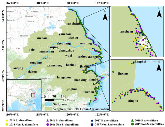
Figure 1.
Location of the study area and sample points.
The total area of wetlands in the Yangtze River Delta region accounts for 10.1% of the country, offshore and coastal wetlands account for 37.4% of the country, and constructed wetlands account for 22.6% of the country. It is unique in the national wetland ecosystem. The coastline in this area is mostly muddy coastline, which provides favorable conditions for the growth of salt marsh vegetation. With the invasion and reproduction of S. alterniflora, it has spread rapidly in the south coast and become a dominant species. In China, Jiangsu Province has the largest area of S. alterniflora. Jiangsu began to introduce S. alterniflora in 1982. Chongming Island in Shanghai is the largest alluvial island, which provides conditions for the growth of S. alterniflora. S. alterniflora was introduced into Zhejiang Province in 1983 [38].
2.2. Dataset
The data used in this study include Landsat time series data, high-resolution images, and field measured data, which are used to obtain training sample points and verification sample points.
2.2.1. Landsat Data and Preprocessing
The study area is covered by five paths/rows (p120r36, p119r37, p118r38, p118r39, and p118r40) of the Landsat worldwide reference system. Based on the Google Earth Engine (GEE) platform, we obtained all available Landsat 5/7/8 surface reflectance (SR) tier 1 products from 1 January 1990 to 31 December 2022. Considering that the growth period of S. alterniflora is from the beginning of April to the end of November, the images of growing season are selected [39,40,41]. Figure 2 shows the image cloud cover and seasonal distribution from 1990 to 2022. Cloud cover less than 20% accounted for 70.5%, cloud cover less than 30% accounted for 80.9%, and cloud cover less than 40% accounted for 89.9%. In order to ensure the existence of images during the growing season and phenological turning point of S. alterniflora, images with less than 5% cloud cover were selected. In addition, some images contaminated by cloud are replaced with the same period images of adjacent years. Due to the failure of the Landsat ETM+ sensor, the image quality of 2012 and 2013 was poor and could not be used. Therefore, the results of 2012 and 2013 were not included in the follow-up spatiotemporal change statistics of S. alterniflora.
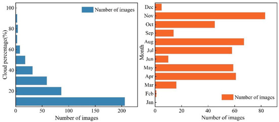
Figure 2.
Cloud cover distribution and seasonal distribution of all images.
2.2.2. Sample Point Data
Based on the field survey of S. alterniflora in typical coastal wetlands of the Yangtze River Delta, we obtained the sample points of Yancheng wetland with coordinate information in 2014 (23 ROIs), Hangzhou Bay wetland in 2016 (32 ROIs) and Chongming Island wetland in 2017 (26 ROIs), respectively. The sampling time occurred during the growing season of S. alterniflora and the sample point size is one pixel unit. Furthermore, field sampling data were utilized as the basis, and high-resolution Google Earth imagery was combined to acquire sample points of S. alterniflora in the coastal wetlands of the Yangtze River Delta. To ensure the random and scientific nature of point selection, ArcGIS 10.2 software was first used to generate a suitable range of random points in the study area. Subsequently, through field investigations and visual interpretation methods, sample points of S. alterniflora and non-S. alterniflora were identified at these random points. These sample points were divided into two groups for training and validation, with each group accounting for 50%. Ultimately, the study obtained the quantity and distribution of sample points as depicted in Table 1 and Figure 1.

Table 1.
Number of sample points in different years.
2.2.3. Auxiliary Data
Climate as an important factor affects the distribution of vegetation communities. In this paper, bioclimatic data with more ecological significance were used to analyze the effect of S. alterniflora distribution on different phenological factors response. The data are from WorldClim, Berkeley University (https://www.worldclim.org/ (accessed on 30 September 2023)) Download Center. The data resolution is 21 km and includes the annual average temperature, annual precipitation, the seasonal changes, and extreme or restricted climate factors. The obtained bioclimatic data are monthly data from 1990 to 2018, which are used to explore the relationship between climate change and the growth of S. alterniflora. X1-10 are indicated in Table 2.
Table 2.
Bioclimatic factors.
3. Methods
In this paper, S. alterniflora was accurately extracted based on the selected high-quality Landsat images, and the ground features were classified based on the phenological information of vegetation. Firstly, the possible growth range of S. alterniflora was determined according to the growing environment conditions in the high soil moisture area. Secondly, the NDVI time series curve of vegetation in the high soil moisture area was constructed to determine the optimal phase of the phenological characteristics difference between S. alterniflora and other vegetation. Finally, a multi-temporal decision tree classification model was constructed to accurately extract S. alterniflora. The overall technical process is shown in Figure 3.
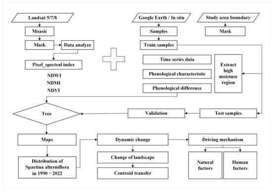
Figure 3.
The workflow for extracting the S. alterniflora cover distribution.
3.1. Extracting High Moisture Region
S. alterniflora grows in the intertidal zone, and the growth environment of wetland vegetation is complex. Therefore, extracting the possible growth area of S. alterniflora is the premise of accurate extraction. Considering the growth environment of S. alterniflora, this study uses the normalized difference moisture index (NDMI), normalized difference water index (NDWI), and normalized difference vegetation index (NDVI) to extract the possible growth area. These three indices are calculated using the following equations:
where Green, Red, NIR, and SWIR are the surface reflectance values of green (525–605 nm), red (630–690 nm), near-infrared (NIR: 760–900 nm), and shortwave infrared (SWIR: 1550–1750 nm) bands.
The NDVI is used to distinguish vegetation from non-vegetation and vegetation is defined as the value of NDVI greater than 0. The NDWI is used to distinguish water body from non-water body and it is non-water body when NDWI is less than 0. The NDMI can effectively extract the water content of the vegetation canopy and can better reflect the difference in swamp vegetation change. According to the statistics of the index values of each sample point, it is found that the moisture index of S. alterniflora is quite different from other ground objects, which provides a threshold reference for determining the high soil moisture area. The high soil moisture area is determined as shown in Equation (4).
where H-moisture areas are areas where S. alterniflora may grow. The high soil moisture area of Hangzhou Bay Wetland includes dry land, paddy field, forest land, and S. alterniflora, and the high soil moisture areas of Yancheng Wetland and Chongming Island include paddy field and S. alterniflora.
3.2. Determining the Optimal Time Phase of Phenological Difference
Due to the influence of cloud cover, the available images cannot reflect the complete phenological characteristics in time series, so it is necessary to improve the quality of time series data. At present, a variety of remote sensing image time series reconstruction methods have been proposed at home and abroad. However, since the reconstruction effect is not obvious, we consider using the data information of adjacent years to fill in the missing data and construct the complete vegetation phenological characteristics.
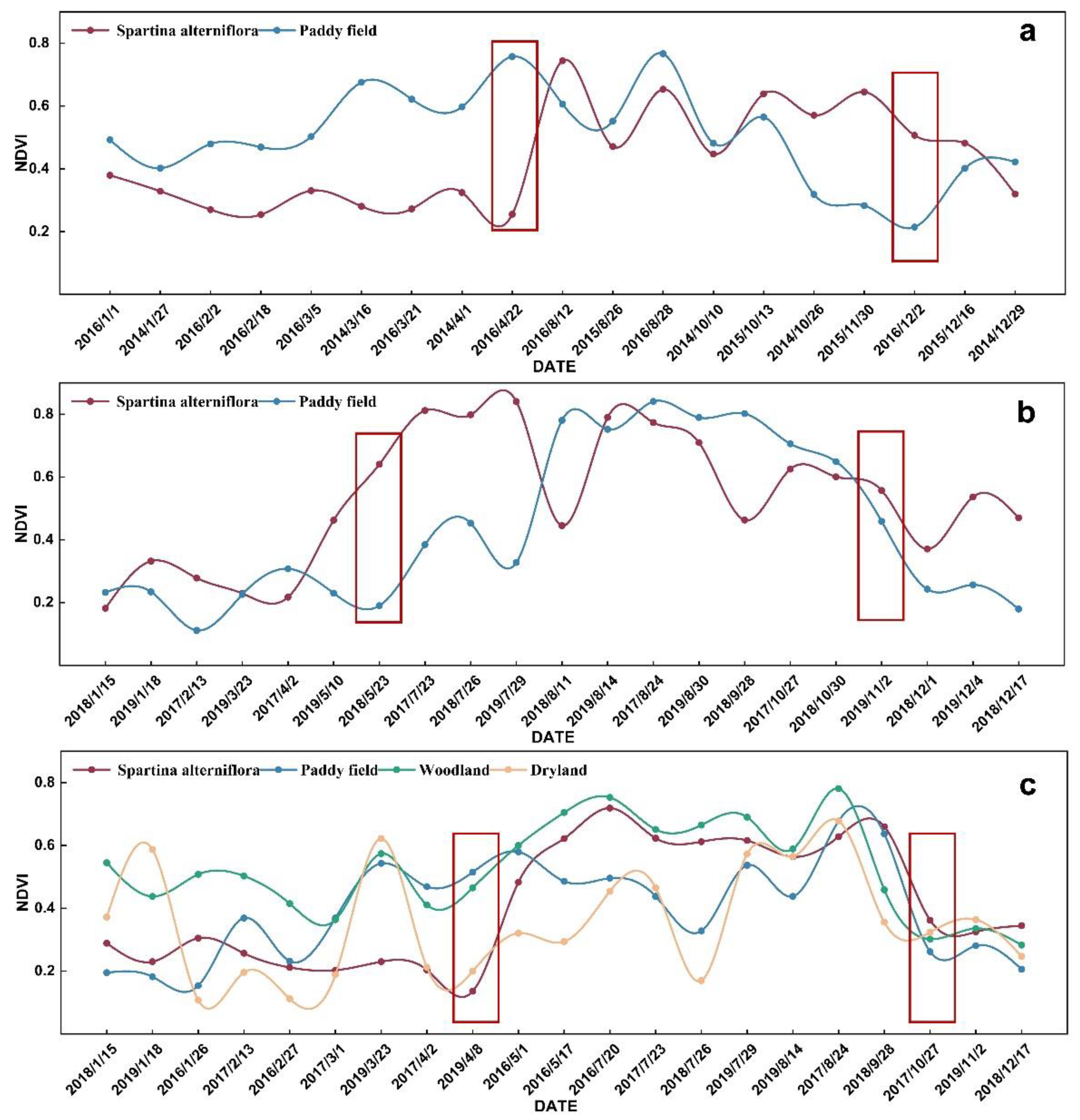
By selecting images of pixels corresponding to sample points in high humidity regions, characteristic indices are computed, and their averages are calculated to construct time series data. Subsequently, the differences in phenological characteristics between S. alterniflora and other vegetation are compared. Figure 4 shows the NDVI change curves of Yancheng Wetland, Chongming Island wetland, and Hangzhou Bay Wetland after data filling. It shows that the vegetation growing season mainly occurs from April to the end of October, and the peak period mainly occurs from July to September. All kinds of NDVI decrease significantly after November. The optimal time phase for the difference between S. alterniflora and paddy field in Yancheng Wetland was the end of April and the end of November. The optimal time phase of the difference between S. alterniflora and paddy field on Chongming Island was reflected in early May and early November. The vegetation growth was not obvious and the vegetation coverage was low in Hangzhou Bay Wetland from January to March, so the difference in NDVI curves among S. alterniflora, dry land, and paddy field was not obvious. From March to April, the curve fluctuates slightly upward. The beginning of May, when the growth difference between S. alterniflora and paddy field is obvious, can be used as the optimal phase. From May to August, the vegetation grows rapidly and the NDVI curve shows a sharp increase trend. At the beginning of the growth season in May, the difference between paddy field and dry land is obvious. The peak value of each ground object in the growth season is reached from July to August, the peak value of forest land NDVI in the growth season is the maximum at the end of August, and the NDVI of various ground objects decreases at the beginning of November. S. alterniflora can be effectively distinguished from forest land in November, and it generally shows late green and wilting characteristics.
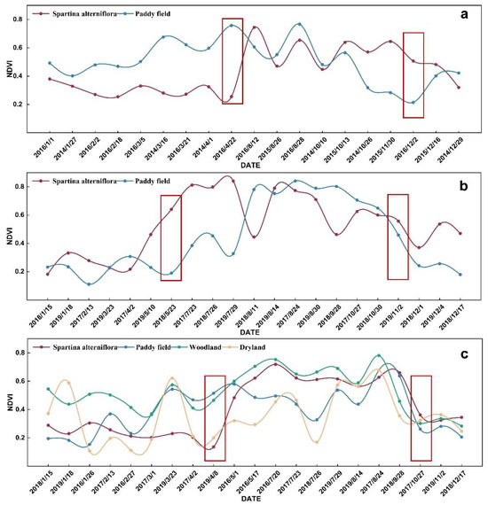
Figure 4.
Comparison of phenological characteristics between S. alterniflora and other vegetation in different subregions: (a) Yancheng Wetland; (b). Chongming Island wetland; (c) Hangzhou Bay Wetland. Note: the red boxes indicate the optimal phenological phases.
3.3. Identifying S. alterniflora
S. alterniflora is a highly competitive invasive plant, which can quickly occupy and replace the local salt marsh vegetation community and form a large area of patches on the ground. Based on 30 m Landsat data, we developed a mapping algorithm of S. alterniflora-based phenology. The algorithm based on phenology adopts two key phenological characteristics of S. alterniflora: late green-up in spring and late senescence in winter. From April to May, S. alterniflora began to turn green later than other vegetation, and its NDVI value was lower. In November, other vegetation begins to wilt and turn yellow, while S. alterniflora can last until the end of November due to its long growth cycle. As can be seen from the line chart, S. alterniflora has the lowest NDVI value in April and the highest NDVI value in early November, which can distinguish it from other vegetation.
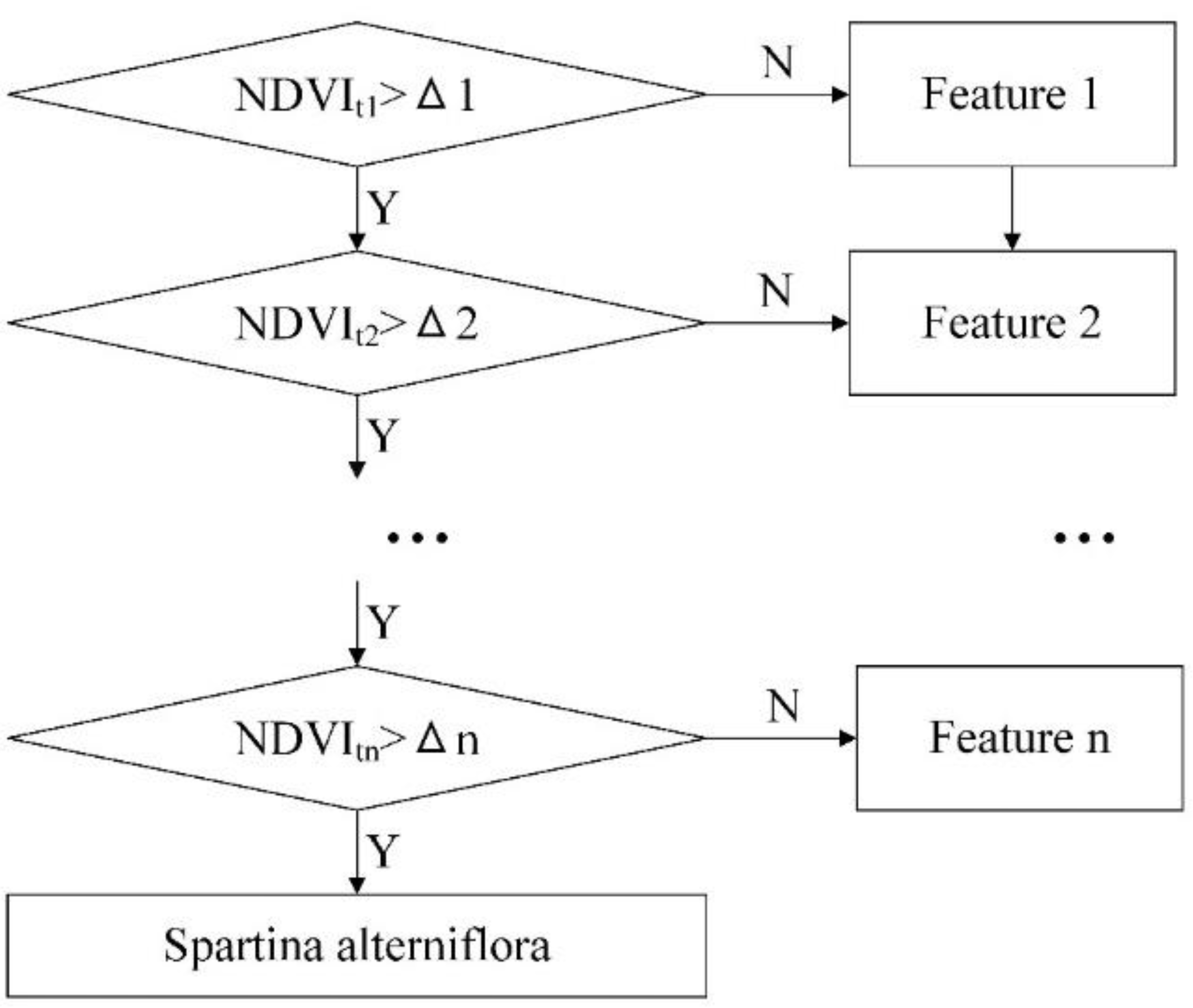
Decision tree is a flexible and intuitive nonparametric rule classifier. It is very useful when integrating multiple variables (such as spectral variables and environmental variables) in the mapping process. It is usually used for wetland classification and monitoring [21,42,43]. According to the constructed NDVI time series curve, the optimal phase of phenological difference was selected. Figure 5 shows the multi-temporal decision tree classification model. t1, t2, and tn are the time phases with the biggest difference between S. alterniflora and a single feature. Δ 1, Δ 2, and Δ n in Figure 5 represent the corresponding NDVI threshold when the classification rule is optimal. The selection of threshold varies with different types of features and different study areas.

Figure 5.
Extracting decision tree of S. alterniflora.
According to the curve in Figure 4, the optimal phase in the Jiangsu region is 22/04 and 26/10, and the thresholds ∆ 1 and ∆ 2 correspond to 0.4 and 0.6, respectively. The optimal time phases in Shanghai are 10/05 and 02/11, and the thresholds ∆ 1 and ∆ 2 correspond to 0.457 and 0.583, respectively. The optimal time phases in Zhejiang are 01/05, 28/09, and 02/11, and the thresholds ∆ 1, ∆ 1, and ∆ 3 correspond to 0.457, 0.637, and 0.336, respectively. The extraction results are shown in red in Figure 6. The method in this paper accurately extracts the range of S. alterniflora, which is distributed along the intertidal zone in strips or sheets, which is consistent with the growth environment of S. alterniflora.
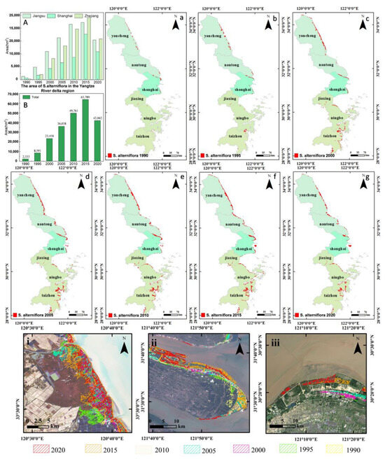
Figure 6.
Mapping S. alterniflora. (A) The change in the total area of S. alterniflora in the Yangtze River Delta. (B) The change in the area of S. alterniflora in each province of the Yangtze River Delta. (a–g) The change in the total distribution of S. alterniflora in the Yangtze River Delta from 1990 to 2022. Local variation map of S. alterniflora: (i) Yancheng; (ii) Chongming Island; (iii) Hangzhou Bay.
4. Results
4.1. S. alterniflora Mapping in the Yangtze River Delta from 1990 to 2022
Many scholars have extracted S. alterniflora from the Yangtze River Delta, but most of them are for a single typical wetland, lacking large-scale distribution statistics [42,43]. This study analyzed the spatial distribution of coastal wetlands in the Yangtze River Delta urban agglomeration. According to the mapping of S. alterniflora from 1990 to 2022 (Figure 6), the area of S. alterniflora in Jiangsu, Shanghai, and Zhejiang in 2022 is 16,848 ha, 17,137 ha, and 10,522 ha, respectively. S. alterniflora invasion primarily occurs in Yancheng Wetland, northern Chongming Island, and the southern coast of Hangzhou Bay. S. alterniflora rapidly expands on Zhejiang and Jiangsu mudflats when not subjected to external factors or interference from other species. Due to the utilization and construction of mudflats and the sedimentation rate of Chongming Island, the expansion rate of S. alterniflora in Shanghai is relatively slow. In Zhejiang, the expansion rate is fastest due to the naturally winding mudflat coastlines. Figure 6i–iii clearly illustrates the expansion of S. alterniflora in Hangzhou Bay as the mudflats accumulate towards the sea. We analyzed the area changes of S. alterniflora in each region and the whole area. In the 1990s and early 21st century, S. alterniflora was just introduced into China, and the small area planted could hardly be detected from Landsat images. The S. alterniflora in the coastal wetland of the Yangtze River Delta expanded from 2333 ha in 1990 to 44,508 ha in 2022.
Due to the high invasion rate of S. alterniflora and the obvious interannual variation of its spatial distribution, it is necessary to conduct accurate monitoring every year. However, due to the number of high-resolution images and the number of field samples, we only assessed the accuracy of cartographic results for some years (2014, 2016, 2017, and 2019) (Table 3). For the validation dataset, we generated random sampling points in ArcGIS and converted them into an export keyhole markup language (KML) file to load into Google Earth. We examined each ROI via visual interpretation of VHSR images and geo referenced photos [44]. VHSR images in Google Earth are an effective data source for verifying land classification results [45,46]. The total number of validation samples for S. alterniflora and non-S. alterniflora were 229 and 192 in 2014, 268 and 217 in 2016, 183 and 189 in 2017, and 227 and 169 in 2019, respectively.
Table 3.
The accuracy of S. alterniflora and non-S. alterniflora in the Yangtze River Delta was evaluated in 2014, 2016, 2017, and 2019. The table also shows the Kappa coefficient and area.
The confusion matrix of S. alterniflora mapping was calculated to estimate the accuracy of the extraction results. The overall accuracies (OA) were 0.93, 0.93, 0.90, and 0.92, and the Kappa coefficients were 0.87, 0.87, 0.81, and 0.84 in 2014, 2016, 2017, and 2019, respectively. The S. alterniflora had producer accuracies (PA) of 0.96, 0.97, 0.91, and 0.96 and user accuracies (UA) of 0.91, 0.91, 0.89, and 0.89 in these four maps.
4.2. Spatiotemporal Expansion Characteristics of S. alterniflora
In order to reflect the change in the S. alterniflora landscape pattern and reveal its change law, we adopted the quantitative method of landscape patterning to reflect the landscape structure composition and spatial configuration characteristics. Based on the patch area, patch shape, and patch aggregation degree, three indexes of landscape area, landscape shape index, and landscape fragmentation degree were selected, all of which were calculated using ArcGIS 10.2 software. The formulas for the calculations are as follows:
where represents the total length of all patch boundaries in the landscape, and represents the total area of the landscape. The shape index indicates the shape changes of the patches, with a larger value indicating a more complex shape.
where represents the fragmentation of landscape , represents the number of patches in landscape , and represents the total area of landscape . The degree of fragmentation represents the degree of landscape separation, reflecting the complexity of the patch structure from the side.
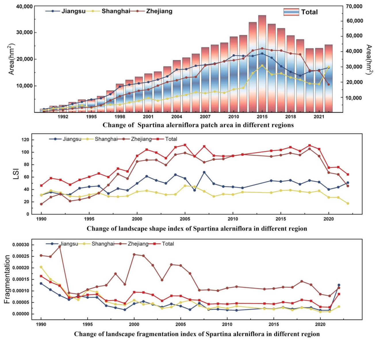
This study analyzed the changes in the landscape index of S. alterniflora invasion from different scales of large scale and three study subareas (Figure 7). The patch area of the three subregions showed an increasing trend. It began to decline in 2015 due to policy and human factors. The same trend was also shown in the large study area. The shape index shows irregular change and fluctuation without obvious regularity. The fragmentation degree is the highest in Zhejiang, which is related to the longest coastline in Zhejiang. The other two areas and the overall fragmentation degree are relatively gentle.

Figure 7.
The expansion dynamics of S. alterniflora during 1990–2022.
In order to reduce the uncertainty caused by image quality or other factors in individual years, we summarized the annual maps of S. alterniflora in multi-year (5-year) intervals. In Table 4, from 1990 to 2000, S. alterniflora invasion was in the early stage. S. alterniflora expanded rapidly on the beaches of Zhejiang and Jiangsu without the interference of foreign factors and other species. Due to the utilization and construction of beaches and the accumulation speed of Chongming Island, S. alterniflora in Shanghai expands slowly. Zhejiang expands fastest due to the natural tortuous muddy coastline. After 2000, the overall expansion rate was relatively stable. By 2015, S. alterniflora began to show negative growth, and the change rate of S. alterniflora decreased significantly.
Table 4.
Dynamic changes in S. alterniflora.
The centroid movement direction of S. alterniflora was calculated using the centroid model. Figure 8 shows the movement of the S. alterniflora center in different areas. The centroid of S. alterniflora in Jiangsu Province moved to the northwest in the first period, and expanded to the southeast in the second period, reflecting the trend of expansion to the sea. In the first period, Shanghai expanded to the southwest. In the second period, it expanded to the northwest due to the increase in S. alterniflora area on Chongming Island. In the third period, it moved to the southeast due to reclamation activities. In the first period, the centroid of S. alterniflora in the north of Zhejiang Province expanded to the southeast. In the second period, due to the rapid expansion of S. alterniflora in Sanmen Bay, it continued to expand to the southeast, but the migration distance of the centroid was short. Affected by some local control activities, the centroid expanded to the northwest in the third period.
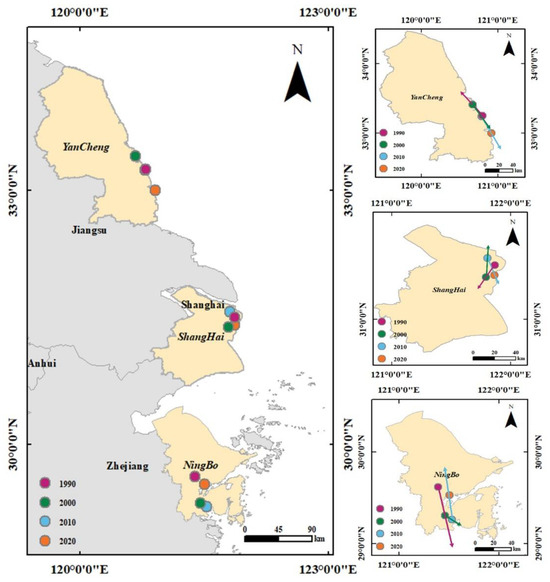
Figure 8.
Centroid movement direction of S. alterniflora in different periods.
4.3. Analysis of Phenological Characteristics and Extraction Accuracy of S. alterniflora at Different Latitudes
The suitable growing area of S. alterniflora spans a large latitude range. In the past few decades, many researchers have studied several characters of S. alterniflora at different latitudes of its original and introduced places, such as stem height and diameter, seed setting rate, and yield. These studies lead us to infer that the rapid spread of S. alterniflora under a wide range of environmental conditions in China is realized through growth characteristic adaptation. As a comprehensive index, the phenological characteristics of S. alterniflora on the latitude gradient, especially the budding and senescence of leaves, are still unclear. Some studies have reported the phenological information of S. alterniflora obtained through field observation or satellite derivation at one or several selected sites. However, these phenological estimates come from different data sources or different phenological algorithms and cannot be compared on the basis of latitude. Based on this, the study investigates the phenological traits of S. alterniflora at various latitudes. Due to the impact of cloud cover and image quality, NDVI is calculated for all available images from 2014 to 2019, and NDVI is extracted for training sample points. The average NDVI changes for each month of the year are then statistically analyzed to obtain a comprehensive overview. The selected seasonal parameters of phenological characteristics mainly include the following: (1) Start of the season: starting from the lowest level on the left side of the time series curve, the time when the left edge increases to the user-defined level. The user-defined level usually refers to a part of the amplitude in the season. (2) End of the season: starting from the lowest level on the right side of the time series curve, the right edge increases to the time corresponding to the user-defined level. (3) Length of the season: the duration from the beginning of the growing season to the end of the growing season, which is numerically equal to the difference between the end time of the season and the start time of the season.
To avoid errors or uncertainties in the annual results, this study has included all images from 2014 to 2019 and has illustrated the seasonal and interannual dynamics of NDVI images for three regions (using a 2-degree latitude interval). From Figure 9, it is evident that the NDVI of Jiangsu, Shanghai, and Zhejiang exhibits distinct seasonal dynamics. The confidence interval in Shanghai is broader, which is linked to the lower quality of images in the study area. The peak period of NDVI in Jiangsu occurs in July, earlier than in other areas of Shanghai and Zhejiang, and the end of the growing season also occurs earlier. The results indicate that, with the increase in latitude, the change in the start of the growing season is not significant, the decline period occurs earlier, and the growing season becomes shorter.
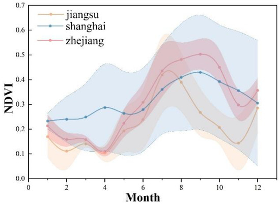
Figure 9.
Phenological characteristics of S. alterniflora at different latitudes.
The detection accuracy of S. alterniflora in the three areas in different years and different methods had no obvious law (Table 5, Table 6 and Table 7). It is worth noting that the multi-year accuracy of the Jiangsu region is slightly higher than that of Shanghai and Zhejiang, which is related to the smooth coastline and the distribution law of S. alterniflora in Zhejiang, and is consistent with the result that the fragmentation of S. alterniflora in Jiangsu is also the lowest in the change in landscape pattern. On the whole, there is little difference between the regional accuracy of Zhejiang and the overall accuracy, which is maintained at the overall accuracy level. The extraction accuracy of Jiangsu is slightly higher than that of the overall region, while the extraction accuracy of S. alterniflora in Shanghai is slightly lower than that of the whole region. The accuracy has no obvious correlation with latitude, but is more related to the distribution characteristics of S. alterniflora.
Table 5.
Etraction accuracy of S. alterniflora in Jiangsu Province in different years.
Table 6.
Etraction accuracy of S. alterniflora in different years in Shanghai.
Table 7.
Etraction accuracy of S. alterniflora in different years in Zhejiang.
4.4. Exploring the Natural Factors Affecting the Growth of S. alterniflora
The climate and bioclimate data of China’s Yangtze River Delta urban agglomeration are obtained by cutting the WorldClim data. Some climate data are completed through band calculation. Subsequently, the correlation between annual forage area changes and multi-year climate change was analyzed. The partial correlation coefficient is a statistical measure used to evaluate the level of correlation between two variables. When dealing with multiple variables, to examine the relationship between any two variables, the other variables are held constant, and the correlation between these two variables is calculated using the partial correlation coefficient. A partial correlation coefficient greater than 0 indicates a positive correlation, less than 0 indicates a negative correlation, and the significance test of the partial correlation coefficient usually adopts the p value test [47]. The partial correlation coefficient between y and X1, as an example:
where represents the partial correlation coefficient between and , after removing the influences of variables . The correlation coefficient formula between the sample and is calculated as:
The formula for testing the partial correlation coefficient is:
where n is the number of samples (n = 27); m is the number of independent variables (m = 9).
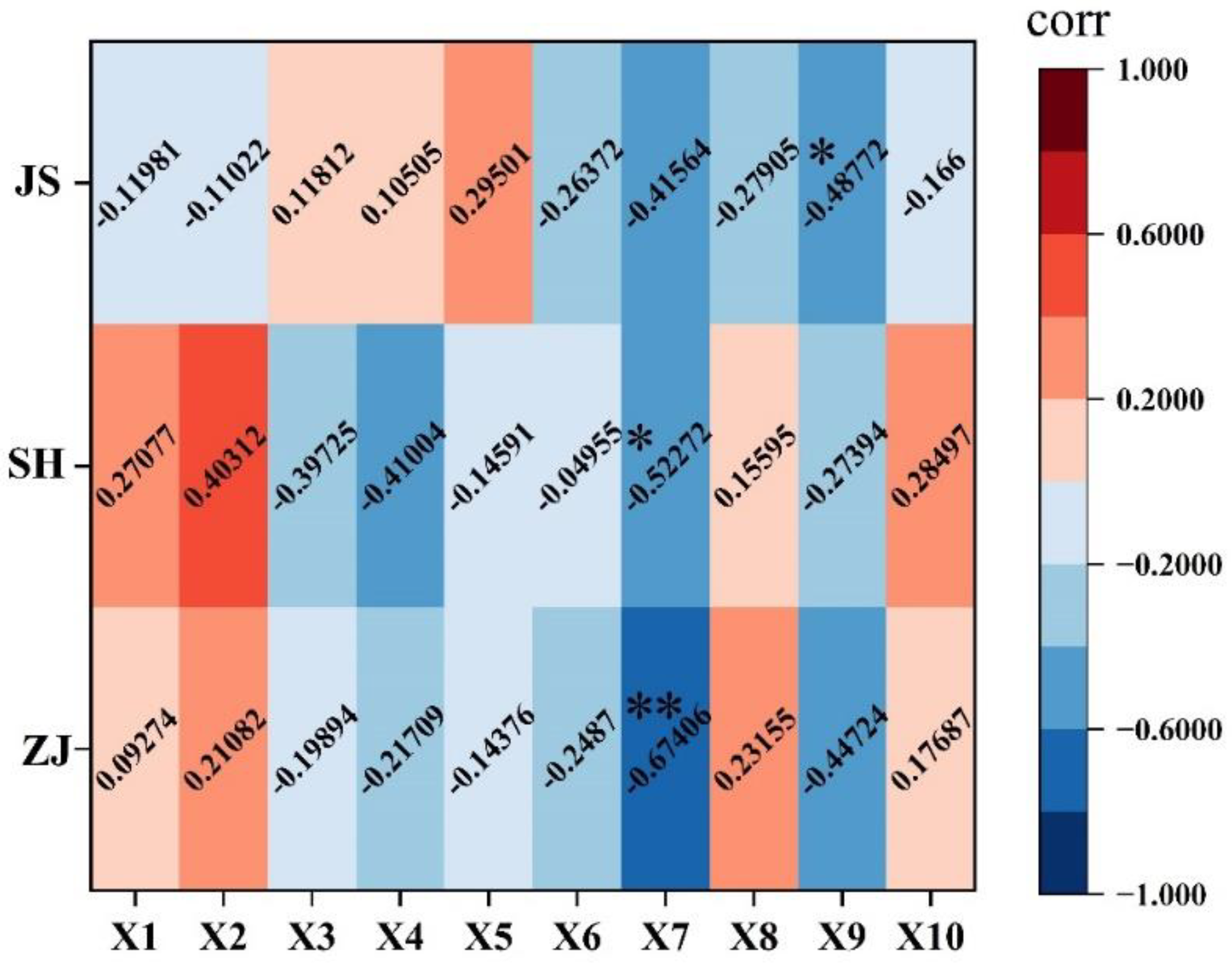
Climate is a significant factor influencing the distribution of vegetation communities, and the adaptability of S. alterniflora to temperature is quite extensive. Therefore, this study selects bioclimatic data with greater ecological significance to analyze the response of S. alterniflora distribution to different phenological factors. To explore the natural factors affecting the growth of S. alterniflora, this study selected 10 climate factors such as average annual precipitation, average annual maximum temperature, average annual minimum temperature, and average annual temperature difference for correlation analysis in the study area (Figure 10). The area of S. alterniflora in Zhejiang Province exhibits a highly significant negative correlation with the coldest month precipitation (X7), with a partial correlation coefficient of −0.67406 and a p value of 0.00215. The area of S. alterniflora in Jiangsu Province is significantly correlated with the temperature of the coldest month, with a partial correlation coefficient of −0.48772 and a p value of 0.04005. Overall, with the increase in latitude, there is no significant change in its correlation. The invasion and area changes of S. alterniflora are mainly influenced by human activities.

Figure 10.
The partial correlation analysis of the S. alterniflora area and climatic factors in different region. Note: * indicates significant correlation at p < 0.05, and ** indicates highly significant correlation at p < 0.01.
5. Discussion
5.1. Growth Characteristics of S. alterniflora
There are many reasons for the spread of S. alterniflora, including natural factors and human factors, such as human introduction, climate, soil, reclamation of tidal flats, and so on. However, it is believed that the strong biological reproductive ability is the main reason for this rapid spread [48]. It has good anti-wave interference and anti-sediment burial performance. S. alterniflora can grow normally when soaked in normal saline for more than 6 h, and can reproduce through sexual and asexual reproduction. It is believed that human reclamation activities have promoted the environmental conditions for the growth of S. alterniflora. The development of the intertidal zone promotes the spread of S. alterniflora. With its growth and proliferation, it accelerates sediment deposition in the intertidal zone. With the passage of time, the sediment deposition becomes higher and higher, and the original growth environment will become a bulge, which will reduce the flooding time, fail to meet the salinity and moisture required for the normal growth of S. alterniflora, and S. alterniflora will gradually wither to death.
5.2. The Uncertainty of Monitoring S. alterniflora Using Remote Sensing Images
To achieve large-scale rapid extraction and long-term monitoring of invasive vegetation in coastal wetlands, we propose a S. alterniflora extraction method based on vegetation phenological characteristics. Through the utilization of landscape pattern indices, centroid models, partial correlation coefficients, and other methods, we conducted an in-depth analysis of the spatiotemporal dynamics of S. alterniflora over more than 30 years. Additionally, we explored the phenological differences of S. alterniflora at different latitudes and evaluated the accuracy of water hyacinth extraction in different regions. In summary, the proposed extraction method of S. alterniflora based on phenological features has achieved good results, and the S. alterniflora extracted in this study also has some errors and limitations. Firstly, the implementation of the phenology-based algorithm in coastal wetlands is limited by high-quality observation during the specific phenological stage, which depends on observation frequency (16 day revisit cycle) and data quality (such as cloud and cloud shadow). Sentinel-2A/2B data together constitute time series data with high time frequency (5 days) and high spatial resolution (10-m, 20-m) [49]. Therefore, Landsat and Sentinel-2 images should be combined in the future mapping and monitoring of rice grass salt marsh. In this study, we used all available Landsat images, which helps to reduce the classification error of annual and multi-year S. alterniflora maps. Secondly, the phenomenon of mixed pixels is inevitable in Landsat 30 m spatial resolution images. The invasion of S. alterniflora into a new pixel generally includes four stages: introduction, establishment, expansion, and domination [50]. In the introduction and establishment stage, the canopy of S. alterniflora is often small, and the area within 30m pixels is small. In the field of land cover mapping, pixel classification of mixed vegetation species is a challenge [51,52,53]. In this paper, our goal is to identify the pixels dominated by S. alterniflora, which means that it will be detected only when S. alterniflora reaches high coverage (relative to pixel size), thus affecting the phenological signal. Finally, due to the special growth environment of S. alterniflora, it will be affected by tidal inundation every day. The imaging time of remote sensing image will be accompanied by different tide level information. When extracting S. alterniflora from high tide level images, it will cause inevitable errors. This is also a problem to be solved in future research. The distribution of S. alterniflora should be accurately extracted in combination with tidal level data.
5.3. Ecological Control Measures of S. alterniflora
These include ploughing and filling, burning, harvesting, freshwater irrigation, shading, and so on. Chemical control mainly involves the application of herbicides; although this means is fast and effective, there will be some drug residues, which may cause environmental pollution and indirectly affect human health. Biological control is mainly based on animal feeding preference (such as leafhoppers) or plant allelopathy. In theory, biological control has a very good application prospect, but there is no very successful precedent. In conclusion, compared with chemical control, physical control of S. alterniflora can effectively control small-area invasion, but there is no more effective method than chemical herbicides for large-area quadrats. The former will not cause environmental pollution, but the control cost is high, while the latter will cause biological and environmental pollution in wetlands, but the control cost is low. Biological control is the most promising, but it may cause biological reinvasion. In the management of S. alterniflora, different management methods should be combined in order to achieve the best effect.
6. Conclusions
In this study, we extracted S. alterniflora from selected high-quality Landsat 5/7/8 images. Based on the phenological information of vegetation, the surface features are classified. Firstly, the study determines potential S. alterniflora growth areas in high-humidity regions by computing spectral characteristics of land cover and vegetation indices, in conjunction with habitat conditions conducive to S. alterniflora growth. Secondly, the NDVI time series curve of vegetation in the high soil moisture area was constructed to determine the phenological characteristics of S. alterniflora and other vegetation. Finally, the multi-temporal decision model was constructed. Based on the strategy tree classification model, S. alterniflora was extracted accurately. The results show that the extraction method in this paper obtains high accuracy, and the annual distribution map of S. alterniflora better reflects the temporal and spatial dynamic changes of S. alterniflora from 1990 to 2022. It can be used to study the driving factors of S. alterniflora dynamic change and quantitatively evaluate the impact of S. alterniflora on biodiversity, carbon cycle and ecosystem services. Our proposed method confirms the potential of S. alterniflora based on phenological feature extraction. The algorithm proposed in this paper establishes a decision tree classification method based on vegetation phenological characteristics based on vegetation phenological growth rules and other auxiliary knowledge, which can better extract the information of S. alterniflora.
Author Contributions
Conceptualization, W.S. and G.Y.; Data curation, Y.Z., K.Z. and C.S.; Formal analysis, S.S., S.Y. and W.G.; Funding acquisition, X.Z., W.S. and G.Y.; Investigation, Y.Z. and S.S.; Methodology, X.Z., Y.Z. and C.S.; Project administration, W.S. and G.Y.; Software, X.Z. and Y.W.; Supervision, W.S. and G.Y.; Validation, C.S. and S.S.; Visualization, Y.Z., K.Z. and Y.W.; Writing—original draft, X.Z. and Y.Z.; Writing—review and editing, X.Z., Y.Z., W.S. and G.Y. All authors have read and agreed to the published version of the manuscript.
Funding
This research was funded by Ningbo Science and Technology Innovation 2025 Major Special Project (Nos. 2022Z189, 2021Z107, 2022Z181), the National Natural Science Foundation of China (No. 42271340, 42122009), and Zhejiang Province “Pioneering Soldier” and “Leading Goose” R&D Project under Grant 2023C01027 and Research project of Hunan Provincial Department of Education under Grant 22C0522.
Data Availability Statement
Data are contains within the article.
Acknowledgments
We express our gratitude to everyone who helped us to successfully complete this research.
Conflicts of Interest
The authors declare no conflicts of interest.
References
- Murray, N.J.; Phinn, S.R.; DeWitt, M.; Ferrari, R.; Johnston, R.; Lyons, M.B.; Clinton, N.; Thau, D.; Fuller, R.A. The Global Distribution and Trajectory of Tidal Flats. Nature 2019, 565, 222–225. [Google Scholar] [CrossRef] [PubMed]
- Wang, X.; Xiao, X.; Zou, Z.; Chen, B.; Ma, J.; Dong, J.; Doughty, R.B.; Zhong, Q.; Qin, Y.; Dai, S. Tracking Annual Changes of Coastal Tidal Flats in China during 1986–2016 through Analyses of Landsat Images with Google Earth Engine. Remote Sens. Environ. 2020, 238, 110987. [Google Scholar] [CrossRef] [PubMed]
- Mao, D.; Liu, M.; Wang, Z.; Li, L.; Man, W.; Jia, M.; Zhang, Y. Rapid Invasion of Spartina Alterniflora in the Coastal Zone of Mainland China: Spatiotemporal Patterns and Human Prevention. Sensors 2019, 19, 2308. [Google Scholar] [CrossRef] [PubMed]
- Liu, C.; Jiang, H.; Zhang, S.; Li, C.; Pan, X.; Lu, J. Expansion and Management Implications of Invasive Alien S. alterniflora in Yancheng Salt Marshes, China. OJE 2016, 6, 113–128. [Google Scholar] [CrossRef]
- Lu, J.; Zhang, Y. Spatial Distribution of an Invasive Plant Spartina Alterniflora and Its Potential as Biofuels in China. Ecol. Eng. 2013, 52, 175–181. [Google Scholar] [CrossRef]
- Chung, C.-H. Forty Years of Ecological Engineering with Spartina Plantations in China. Ecol. Eng. 2006, 27, 49–57. [Google Scholar] [CrossRef]
- Wu, Y.; Xiao, X.; Chen, R.; Ma, J.; Wang, X.; Zhang, Y.; Zhao, B.; Li, B. Tracking the Phenology and Expansion of Spartina Alterniflora Coastal Wetland by Time Series MODIS and Landsat Images. Multimed. Tools Appl. 2020, 79, 5175–5195. [Google Scholar] [CrossRef]
- Song, S.; Wu, Z.; Wang, Y.; Cao, Z.; He, Z.; Su, Y. Mapping the Rapid Decline of the Intertidal Wetlands of China Over the Past Half Century Based on Remote Sensing. Front. Earth Sci. 2020, 8, 16. [Google Scholar] [CrossRef]
- Zhang, D.; Hu, Y.; Liu, M.; Chang, Y.; Yan, X.; Bu, R.; Zhao, D.; Li, Z. Introduction and Spread of an Exotic Plant, Spartina Alterniflora, Along Coastal Marshes of China. Wetlands 2017, 37, 1181–1193. [Google Scholar] [CrossRef]
- Sun, Z.; Sun, W.; Tong, C.; Zeng, C.; Yu, X.; Mou, X. China’s Coastal Wetlands: Conservation History, Implementation Efforts, Existing Issues and Strategies for Future Improvement. Environ. Int. 2015, 79, 25–41. [Google Scholar] [CrossRef]
- Liu, Y.-F.; Ma, J.; Wang, X.-X.; Zhong, Q.-Y.; Zong, J.-M.; Wu, W.-B.; Wang, Q.; Zhao, B. Joint Effect of Spartina Alterniflora Invasion and Reclamation on the Spatial and Temporal Dynamics of Tidal Flats in Yangtze River Estuary. Remote Sens. 2020, 12, 1725. [Google Scholar] [CrossRef]
- Tang, C. Ecological Control of S. alterniflora and Improvement of Birds Habitats in Chongming Dongtan Wetland, Shanghai. Wetl. Sci. Manag. 2016, 12, 4–8. [Google Scholar]
- Feng, J.; Huang, Q.; Qi, F.; Guo, J.; Lin, G. Utilization of Exotic Spartina Alterniflora by Fish Community in the Mangrove Ecosystem of Zhangjiang Estuary: Evidence from Stable Isotope Analyses. Biol. Invasions 2015, 17, 2113–2121. [Google Scholar] [CrossRef]
- Chu, Z.; Yang, X.; Feng, X.; Fan, D.; Li, Y.; Shen, X.; Miao, A. Temporal and Spatial Changes in Coastline Movement of the Yangtze Delta during 1974–2010. J. Asian Earth Sci. 2013, 66, 166–174. [Google Scholar] [CrossRef]
- Ouyang, Z.-T.; Gao, Y.; Xie, X.; Guo, H.-Q.; Zhang, T.-T.; Zhao, B. Spectral Discrimination of the Invasive Plant Spartina Alterniflora at Multiple Phenological Stages in a Saltmarsh Wetland. PLoS ONE 2013, 8, e67315. [Google Scholar] [CrossRef]
- Pendleton, L.; Donato, D.C.; Murray, B.C.; Crooks, S.; Jenkins, W.A.; Sifleet, S.; Craft, C.; Fourqurean, J.W.; Kauffman, J.B.; Marbà, N. Estimating Global “Blue Carbon” Emissions from Conversion and Degradation of Vegetated Coastal Ecosystems. PLoS ONE 2012, 7, e43542. [Google Scholar] [CrossRef]
- Chung, C.; Zhuo, Z.; Xu, G. Creation of Spartina Plantations for Reclaiming Dongtai, China, Tidal Flats and Offshore Sands. Ecol. Eng. 2004, 23, 135–150. [Google Scholar] [CrossRef]
- Chen, L.; Ren, C.; Zhang, B.; Li, L.; Wang, Z.; Song, K. Spatiotemporal Dynamics of Coastal Wetlands and Reclamation in the Yangtze Estuary During Past 50 Years (1960s–2015). Chin. Geogr. Sci. 2018, 28, 386–399. [Google Scholar] [CrossRef]
- Wang, W.; Liu, H.; Li, Y.; Su, J. Development and Management of Land Reclamation in China. Ocean Coast. Manag. 2014, 102, 415–425. [Google Scholar] [CrossRef]
- Betbeder, J.; Rapinel, S.; Corgne, S.; Pottier, E.; Hubert-Moy, L. TerraSAR-X Dual-Pol Time-Series for Mapping of Wetland Vegetation. ISPRS J. Photogramm. Remote Sens. 2015, 10, 90–98. [Google Scholar] [CrossRef]
- Adam, E.; Mutanga, O.; Rugege, D. Multispectral and Hyperspectral Remote Sensing for Identification and Mapping of Wetland Vegetation: A Review. Wetl. Ecol Manag. 2010, 18, 281–296. [Google Scholar] [CrossRef]
- Moffett, K.B.; Nardin, W.; Silvestri, S.; Wang, C.; Temmerman, S. Multiple Stable States and Catastrophic Shifts in Coastal Wetlands: Progress, Challenges, and Opportunities in Validating Theory Using Remote Sensing and Other Methods. Remote Sens. 2015, 7, 10184–10226. [Google Scholar] [CrossRef]
- Zhang, Y.; Lu, D.; Yang, B.; Sun, C.; Sun, M. Coastal Wetland Vegetation Classification with a Landsat Thematic Mapper Image. Int. J. Remote Sens. 2011, 32, 545–561. [Google Scholar] [CrossRef]
- Yang, G.; Huang, K.; Sun, W.; Meng, X.; Mao, D.; Ge, Y. Enhanced Mangrove Vegetation Index Based on Hyperspectral Images for Mapping Mangrove. ISPRS J. Photogramm. Remote Sens. 2022, 189, 236–254. [Google Scholar] [CrossRef]
- Cheng, S.; Yang, X.; Yang, G.; Chen, B.; Chen, D.; Wang, J.; Ren, K.; Sun, W. Using ZY1-02D Satellite Hyperspectral Remote Sensing to Monitor Landscape Diversity and Its Spatial Scaling Change in the Yellow River Estuary. Int. J. Appl. Earth Obs. Geoinf. 2024, 128, 103716. [Google Scholar] [CrossRef]
- Gilmore, M.S.; Wilson, E.H.; Barrett, N.; Civco, D.L.; Prisloe, S.; Hurd, J.D.; Chadwick, C. Integrating Multi-Temporal Spectral and Structural Information to Map Wetland Vegetation in a Lower Connecticut River Tidal Marsh. Remote Sens. Environ. 2008, 112, 4048–4060. [Google Scholar] [CrossRef]
- Klemas, V.V. Coastal and Environmental Remote Sensing from Unmanned Aerial Vehicles: An Overview. J. Coast. Res. 2015, 31, 1260–1267. [Google Scholar] [CrossRef]
- Wan, H.; Wang, Q.; Jiang, D.; Fu, J.; Yang, Y.; Liu, X. Monitoring the Invasion of Spartina Alterniflora Using Very High Resolution Unmanned Aerial Vehicle Imagery in Beihai, Guangxi (China). Sci. World J. 2014, 2014, 638296. [Google Scholar] [CrossRef]
- Liu, M.; Li, H.; Li, L.; Man, W.; Jia, M.; Wang, Z.; Lu, C. Monitoring the Invasion of Spartina Alterniflora Using Multi-Source High-Resolution Imagery in the Zhangjiang Estuary, China. Remote Sens. 2017, 9, 539. [Google Scholar] [CrossRef]
- Kou, W.; Xiao, X.; Dong, J.; Gan, S.; Zhai, D.; Zhang, G.; Qin, Y.; Li, L. Mapping Deciduous Rubber Plantation Areas and Stand Ages with PALSAR and Landsat Images. Remote Sens. 2015, 7, 1048–1073. [Google Scholar] [CrossRef]
- Heumann, B.W. An Object-Based Classification of Mangroves Using a Hybrid Decision Tree—Support Vector Machine Approach. Remote Sens. 2011, 3, 2440–2460. [Google Scholar] [CrossRef]
- Li, N.; Li, L.; Zhang, Y.; Wu, M. Monitoring of the Invasion of Spartina Alterniflora from 1985 to 2015 in Zhejiang Province, China. BMC Ecol. 2020, 20, 7. [Google Scholar] [CrossRef] [PubMed]
- Wang, A.; Chen, J.; Jing, C.; Ye, G.; Wu, J.; Huang, Z.; Zhou, C. Monitoring the Invasion of Spartina Alterniflora from 1993 to 2014 with Landsat TM and SPOT 6 Satellite Data in Yueqing Bay, China. PLoS ONE 2015, 10, e0135538. [Google Scholar] [CrossRef] [PubMed]
- Tian, J.; Wang, L.; Yin, D.; Li, X.; Diao, C.; Gong, H.; Shi, C.; Massimo, M.; Ge, Y.; Ni, S.; et al. Development of Spectral-Phenological Features for Deep Learning to Understand Spartina Alterniflora Invasion. Remote Sens. Environ. 2020, 242, 111745. [Google Scholar] [CrossRef]
- Zhang, X.; Xiao, X.; Wang, X.; Xu, X.; Chen, B.; Wang, J.; Ma, J.; Zhao, B.; Li, B. Quantifying Expansion and Removal of Spartina Alterniflora on Chongming Island, China, Using Time Series Landsat Images during 1995–2018. Remote Sens. Environ. 2020, 247, 111916. [Google Scholar] [CrossRef] [PubMed]
- Sun, C.; Li, J.; Liu, Y.; Liu, Y.; Liu, R. Plant Species Classification in Salt Marshes Using Phenological Parameters Derived from Sentinel-2 Pixel-Differential Time-Series. Remote Sens. Environ. 2021, 256, 112320. [Google Scholar] [CrossRef]
- Zuo, P.; Zhao, S.; Liu, C.; Wang, C.; Liang, Y. Distribution of Spartina Spp. along China’s Coast. Ecol. Eng. 2012, 40, 160–166. [Google Scholar] [CrossRef]
- Hu, Y.; Tian, B.; Yuan, L.; Li, X.; Huang, Y.; Shi, R.; Jiang, X.; Wang, L.; Sun, C. Mapping Coastal Salt Marshes in China Using Time Series of Sentinel-1 SAR. ISPRS J. Photogramm. Remote Sens. 2021, 173, 122–134. [Google Scholar] [CrossRef]
- Gao, Z.G.; Zhang, L.Q. Multi-Seasonal Spectral Characteristics Analysis of Coastal Salt Marsh Vegetation in Shanghai, China. Estuar. Coast. Shelf Sci. 2006, 69, 217–224. [Google Scholar] [CrossRef]
- Baker, C.; Lawrence, R.; Montagne, C.; Patten, D. Mapping Wetlands and Riparian Areas Using Landsat ETM+ Imagery and Decision-Tree-Based Models. Wetlands 2006, 26, 465–474. [Google Scholar] [CrossRef]
- Davranche, A.; Lefebvre, G.; Poulin, B. Wetland Monitoring Using Classification Trees and SPOT-5 Seasonal Time Series. Remote Sens. Environ. 2010, 114, 552–562. [Google Scholar] [CrossRef]
- Zhang, W.; Zeng, C.; Tong, C.; Zhang, Z.; Huang, J. Analysis of the Expanding Process of the Spartina Alterniflora Salt Marsh in Shanyutan Wetland, Minjiang River Estuary by Remote Sensing. Procedia Environ. Sci. 2011, 10, 2472–2477. [Google Scholar] [CrossRef]
- Ma, Z.; Gan, X.; Cai, Y.; Chen, J.; Li, B. Effects of Exotic Spartina Alterniflora on the Habitat Patch Associations of Breeding Saltmarsh Birds at Chongming Dongtan in the Yangtze River Estuary, China. Biol. Invasions 2011, 13, 1673–1686. [Google Scholar] [CrossRef]
- Olofsson, P.; Foody, G.M.; Herold, M.; Stehman, S.V.; Woodcock, C.E.; Wulder, M.A. Good Practices for Estimating Area and Assessing Accuracy of Land Change. Remote Sens. Environ. 2014, 148, 42–57. [Google Scholar] [CrossRef]
- Kennedy, R.E.; Yang, Z.; Cohen, W.B. Detecting Trends in Forest Disturbance and Recovery Using Yearly Landsat Time Series: 1. LandTrendr—Temporal Segmentation Algorithms. Remote Sens. Environ. 2010, 114, 2897–2910. [Google Scholar] [CrossRef]
- Huang, H.G.; Samuel, N.G.; Jeffrey, G.M.; Nancy, T.; Zhu, Z.l.; James, E.V. An Automated Approach for Reconstructing Recent Forest Disturbance History Using Dense Landsat Time Series Stacks. Remote Sens. Environ. 2010, 114, 183–198. [Google Scholar] [CrossRef]
- Jing, J.; Deng, Q.; He, C. Spatiotemporal Evolution of NDVl and Its Climatic Driving Factors in the Southwest Karst Area from 1999 to 2019. Res. Soil Water Conserv. 2023, 30, 232–239. [Google Scholar]
- Zhang, R.S.; Shen, Y.M.; Lu, L.Y.; Yan, S.G.; Wang, Y.H.; Li, J.L.; Zhang, Z.L. Formation of Spartina Alterniflora Salt Marshes on the Coast of Jiangsu Province, China. Ecol. Eng. 2004, 23, 95–105. [Google Scholar] [CrossRef]
- Griffiths, P.; Nendel, C.; Hostert, P. Intra-Annual Reflectance Composites from Sentinel-2 and Landsat for National-Scale Crop and Land Cover Mapping. Remote Sens. Environ. 2019, 220, 135–151. [Google Scholar] [CrossRef]
- Vaz, A.S.; Alcaraz-Segura, D.; Campos, J.C.; Vicente, J.R.; Honrado, J.P. Managing Plant Invasions through the Lens of Remote Sensing: A Review of Progress and the Way Forward. Sci. Total Environ. 2018, 642, 1328–1339. [Google Scholar] [CrossRef]
- Herold, M.; Mayaux, P.; Woodcock, C.E.; Baccini, A.; Schmullius, C. Some Challenges in Global Land Cover Mapping: An Assessment of Agreement and Accuracy in Existing 1 Km Datasets. Remote Sens. Environ. 2008, 112, 2538–2556. [Google Scholar] [CrossRef]
- Gong, P.; Wang, J.; Yu, L.; Zhao, Y.; Zhao, Y.; Liang, L.; Niu, Z.; Huang, X.; Fu, H.; Liu, S.; et al. Finer Resolution Observation and Monitoring of Global Land Cover: First Mapping Results with Landsat TM and ETM+ Data. Int. J. Remote Sens. 2013, 34, 2607–2654. [Google Scholar] [CrossRef]
- Wang, J.; Xiao, X.; Qin, Y.; Dong, J.; Geissler, G.; Zhang, G.; Cejda, N.; Alikhani, B.; Doughty, R.B. Mapping the Dynamics of Eastern Redcedar Encroachment into Grasslands during 1984–2010 through PALSAR and Time Series Landsat Images. Remote Sens. Environ. 2017, 190, 233–246. [Google Scholar] [CrossRef]


Disclaimer/Publisher’s Note: The statements, opinions and data contained in all publications are solely those of the individual author(s) and contributor(s) and not of MDPI and/or the editor(s). MDPI and/or the editor(s) disclaim responsibility for any injury to people or property resulting from any ideas, methods, instructions or products referred to in the content. |
© 2024 by the authors. Licensee MDPI, Basel, Switzerland. This article is an open access article distributed under the terms and conditions of the Creative Commons Attribution (CC BY) license (https://creativecommons.org/licenses/by/4.0/).