Abstract
Accurate mapping of forest habitats, especially in NATURA sites, is essential information for forest monitoring and sustainable management but also for habitat characterisation and ecosystem functioning. Remote sensing data and spatial modelling allow accurate mapping of the presence and distribution of tree species and habitats and are valuable tools for the long-term assessment of habitat status required by the European Commission. In order to serve the above, the present study aims to propose a methodology to accurately map the spatial distribution of forest habitats in three NATURA2000 sites of Cyprus by employing Sentinel-1 and Sentinel-2 data as well as topographic features using the Google Earth Engine (GEE). A pivotal aspect of the methodology identified was that the best band combination of the Random Forest (RF) classifier achieves the highest performance for mapping the dominant habitats in the three case studies. Specifically, in the Akamas region, eight habitat types have been mapped, in Paphos nine and six in Troodos. These habitat types are included in three of the nine habitat groups based on the EU’s Habitat Directive: the sclerophyllous scrub, rocky habitats and caves and forests. The results show that using the RF algorithm achieves the highest performance, especially using Dataset 6, which is based on S2 bands, spectral indices and topographical features, and Dataset 13, which includes S2, S1, spectral indices and topographical features. These datasets achieve an overall accuracy (OA) of approximately 91–94%. In contrast, Dataset 7, which includes only S1 bands and Dataset 9, which combines S1 bands and spectral indices, achieve the lowest performance with an OA of approximately 25–43%.
1. Introduction
Forest habitat mapping constitutes a critical pillar of forest management, biodiversity conservation, ecological monitoring and forestry. Forest habitats were mainly mapped through field surveys and manual identification [1]. This involved personal effort from foresters observing and identifying habitats based on their characteristics and knowledge of local flora through site visits. The need for more efficient and large-scale techniques of forest habitat classification grew over time, leading to the development of aerial photography in the mid-20th century [2] and eventually to the advent of satellite technology in the late 20th century, resulting in the advancement in forest habitats classification [3]. Accurate forest habitat identification is achieved through the capability of satellite sensors to retrieve information in different parts of the electromagnetic spectrum such as the visible, near-infrared and shortwave infrared. Over the past few decades, the science of remote sensing has expanded in different forest applications, such as fire damage assessment [4], time series of forest seasonality [5] and even calculating forest canopy density [6]. These different forestry applications utilising remote sensing are essential for monitoring forest areas, especially when dealing with NATURA 2000 habitats. The importance of monitoring these sites is that NATURA is the world’s largest coordinated network of protected areas, extending across all 27 EU Member States on land and at sea. The areas within NATURA 2000 are designated under the Birds (2009/147/EC) and Habitats Directives (92/43/EEC), indicating their importance for systematic monitoring [7]. In Cyprus, this network covers 63 sites covering 10,145 km2, ranking it among the top EU countries regarding the percentage of the land area included within the NATURA 2000 network. Moreover, 75% of state forest land is included in the network, in which 26 sites host significant forest areas [8] and more than 700 different plant species as recorded in the Red Data Book of the Flora of Cyprus [9]. Consequently, the need to systematically monitor these areas is vital for several reasons, such as biodiversity conservation, habitat assessment, policy and management [10].
Various plant classification techniques are currently available; thus, selecting the most appropriate method depends on the site-specific characteristics. Traditional spatial-based classification techniques such as Random Forest (RF) [11,12] and Support Vector Machine (SVM) [13] have been broadly exploited in numerous studies where comparisons with other classifications have been conducted [14,15,16]. However, recent advancements in machine learning (ML) have led to the development of deep learning classification techniques for plant species classification, such as Convolutional Neural Networks (CNN) [17,18], Long Short-Term Memory Networks (LSTMs) [19,20], Recurrent Neural Networks (RNNs) [21,22] and Multilayer Perceptrons (MLPs) [23]. For this study, the Random Forest was selected since it is considered to be one of the most widely used algorithms for land cover classification using remote sensing data [24,25,26,27,28,29,30]. This is confirmed by the meta-analysis conducted by Tamiminia et al. 2020 [31], based on 349 peer-reviewed GEE articles published in 146 journals between 2010 and October 2019, showing that the Random Forest was the most frequently used algorithm for satellite imagery processing. This is due to effectively managing outliers and datasets characterised by significant noise. Also, it features robust performance in high-dimensional and multisource data. Furthermore, in numerous studies, the RF has demonstrated higher accuracy in comparison with other widely used classifiers such as Support Vector Machine (SVM), Gradient Tree Boost, Classification and Regression Trees (CART) [31,32]. In addition, another advantage of the RF is the enhanced processing speed achieved through the selection of essential variables [33,34].
Another crucial factor for the study area is where the classifier is utilised. Diverse types of vegetation such as grasslands [35,36], shrubs [37,38], mangroves [39,40], wetlands [41,42], croplands [43], tundra [44] and forests [45] may require different remote sensing classification methods due to their unique characteristics. The challenges posed by data complexity and availability are crucial across these ecosystems. In recent years, the rise of cloud-based platforms, particularly Google Earth Engine (GEE), has brought significant advancements in forest species and habitat classification, providing access to vast datasets of satellite images, data analysis and visualisation tools [46]. GEE has been widely used due to its advantage of handling large datasets and performing complex analyses, while at the same time providing a set of state-of-the-art classifiers for pixel-based classification that can be utilised for forest habitats classification in a variety of complex ecosystems [21,47,48]. For instance, a study conducted in Indonesia compared the three ML classifiers available in GEE, the SVM, RF and the Classification and Regression Trees (CART) for discriminating mangroves and non-mangroves has led to the outperformance of SVM compared to the other classifiers [49].
The mapping of NATURA 2000 areas utilising satellite remote sensing is critical for monitoring changes in these habitats over time. Numerous studies in different regions in Europe have examined how these habitats can be mapped [50,51,52,53,54]. One study introduced an ML framework for the NATURA 2000 habitat monitoring in Germany exploiting readily available MODIS (Moderate Resolution Imaging Spectroradiometer) surface reflectance data [55], whereas a study in Poland aimed to classify NATURA 2000 grassland habitats exploiting hyperspectral data fused with topographic indices [56]. Another study in Central Slovakia utilised a phytosociological approach integrated with Sentinel-2 satellite data with software that they created to differentiate the various NATURA 2000 habitats [57]. Regarding the Cyprus territory, according to the literature, only two studies were focused on mapping NATURA 2000 sites in Cyprus. However, the first study dates from 2008, utilising a multispectral image from QuickBird satellite focusing on a small area west of Nicosia [58]. Although the second study was newer (2018), focusing on multiple NATURA 2000 sites, it implemented only photointerpretation using orthophotos with some supplementary materials (i.e., Google Earth imagery, etc.) [45]. These two studies highlighted the need for more research on mapping NATURA 2000 habitats in Cyprus, underscoring the need for further studies to understand and preserve the unique biodiversity and habitats within these protected areas. These findings show a profound gap in mapping forest habitats through satellite images in Cyprus.
The study aimed to accurately map the spatial distribution of forest habitats in NATURA2000 sites using different types of satellite data (optical, RADAR) and topographic features in the Google Earth Engine (GEE) environment. More specifically, the objectives of the research were: (1) to examine the impact of using spectral indices and the backscatter coefficient for forest habitats mapping at a regional scale, (2) to determine the relationship between the time of data collection (month of the year) and the accuracy of mapping and (3) to investigate the possibility of mapping the spatial distribution of forest habitats in the study areas with high accuracy. This will enable a better understanding of the dynamics of these areas and will serve as a management tool towards the preservation of these habitats. Furthermore, the proposed methodology is a valuable tool for Article 17 of the Habitats Directive, which focuses on updating the conservation status of habitats every six years.
2. Materials and Methods
2.1. Study Area
For the purposes of this study, three NATURA2000 sites were selected, which are the Paphos (Special Protection Area), Troodos (CY5000004) and Akamas Peninsula (CY4000010), as shown in Figure 1.
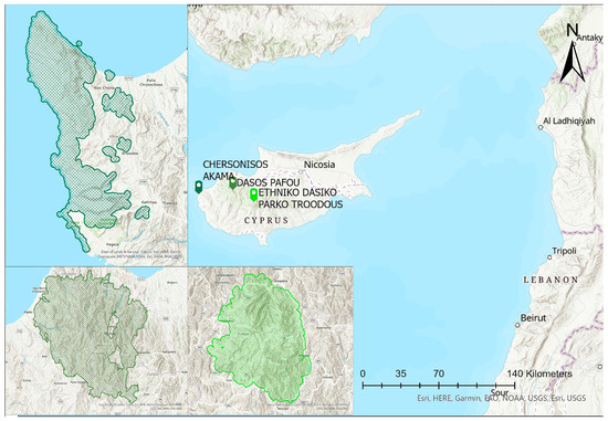
Figure 1.
Location of the examined NATURA 2000 regions.
2.1.1. Paphos State Forest: CY2000006
Paphos State Forest is located in the northwest part of the Troodos range, and it covers 602 km2. It is one of the most crucial state forests of the island because it includes extensive natural habitats that comprise many flora and fauna species. Its significance lies in the fact that it constitutes the most extensive continuous forest ecosystem in Cyprus, with the largest pine forest on the island, the unique endemic cedar forest (a priority habitat) and several other forest habitats. Apart from that, the area’s avifauna contains 96 bird species and given its significance, has been suggested as a Special Protection Area (SPA). Furthermore, it is essential because it is the only biotope that hosts the endemic Ovis orientalis ophion and supports the largest population of Coluber cypriensis (Cyprus whip snake) [59].
2.1.2. Akamas Peninsula (CY4000010)
Akamas is situated in the westernmost part of the island and presents high ecological value due to its geographical position and landscape diversity. Specifically, the Akamas Peninsula represents well-conserved Eastern Mediterranean ecosystems, including high habitat and species diversity. Akamas NATURA region covers 179 km2 but this study examines only the terrestrial area, which covers an area of 124 km2. Furthermore, it is one of the only three sites in Cyprus with the endemic priority serpentinophilous grasslands habitat. In regard to fauna, Akamas is vital for the avifauna, and especially for the migratory birds [60].
2.1.3. Troodos (CY5000004)
The National Forest Park of Troodos is situated at the centre of the Troodos massif and covers an area of 90 km2. The area’s importance lies in the large number of plants and endemic plants hosted in the area compared to any other area of the island. Also, it has been characterised as one of the 13 “Plant Diversity Hot Spots” in the Mediterranean region. Furthermore, we have to highlight that the Pallas’ pine forests (priority habitat) are extended only on Troodos, while the stinking juniper (Juniperus foetidissima) woods (priority habitat) are confined to this area [61].
2.2. Datasets
The mapping of the primary forest habitats in the three NATURA 2000 regions was conducted using Sentinel-1 and Sentinel-2 satellite images in combination with auxiliary data for elevation and slope, which are derived from DEM. For each case study, we use habitat types according to the EU Habitat Directive, which includes nine habitat groups: (1) coastal and halophytic habitats, (2) coastal sand dunes and inland dunes, (3) freshwater habitats, (4) temperate heath and scrub, (5) sclerophyllous scrub, (6) natural and semi-natural grassland formations, (7) raised bogs and mires and fens, (8) rocky habitats and caves, (9) forests. For this study, habitat types were selected from groups 5, 8 and 9, with the selected habitats for each case study detailed in Table 1.

Table 1.
Habitat types were mapped in each case study according to the EU Habitat.
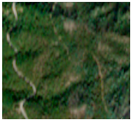
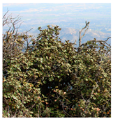
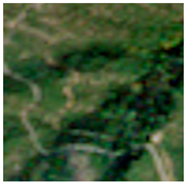
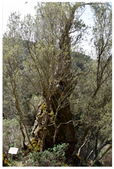
The collection of the samples for the forest habitats was conducted by the Department of Forests in Cyprus through site visits in the framework of the IP Physics program. Table 2 presents some examples from the habitat types and their corresponding Sentinel-2 images.
Table 2.
Samples of habitat types were mapped. The table presents the name of the habitat type, images from the site visits and the corresponding Sentinel-2 image.
Furthermore, the processing of the images, as presented in Figure 2, was conducted in the Google Earth Engine (GEE) environment. The GEE is a planetary scale platform for analysing and visualising geospatial data. In this study, the GEE was utilised to create a process for obtaining the band reflectance values, vegetation indices and backscattering coefficients from Sentinel-1 and Sentinel-2 in order to employ the pixel-based Random Forest (RF) classifier for the mapping of the forest habitats in the study areas. An overview of the satellite sensors is presented in the following sub-sections.
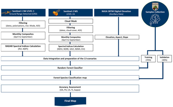
Figure 2.
Flow chart of the classification of the habitats in the three NATURA2000 regions.
2.2.1. Sentinel-1
The Sentinel-1 mission is a European SAR satellite comprising a constellation of two polar-orbiting satellites (Sentinel-1A and -1B). It also uses a single C-band Synthetic Aperture Radar (SAR) sensor, which can penetrate clouds with a spatial resolution of 10, 25, or 40 m and a temporal resolution of 6–12 days at a central frequency of 5.405 GHz. Furthermore, these satellites are enabled to acquire data in four modes: strip map (SM), interferometric wide swath (IW), extra-wide swath (EW) and wave mode (WV) [62,63].
This study used the Sentinel-1 Ground Range Detected (GRD) product considering the interferometric wide swath (IW) mode in the ascending and descending view angle. Furthermore, the horizontal/vertical-transmit/receive (HV) and the vertical/vertical-transmit/receive (VV) were processed. On 3 August 2022, the European Commission and ESA (European Space Agency) announced the end of the Sentinel-1B satellite mission; therefore, data collected after 21 December 2021 were processed only for Sentinel-1A [64]. In addition, all images from May to September 2022 were selected and preprocessed by the Sentinel-1 toolbox. The preprocessed actions included thermal noise removal, radiometric calibration, terrain correction and the conversion of backscatter coefficients (σ0) to decibels (dB).
2.2.2. Sentinel-2
ESA launched the Sentinel-2 mission, an optical platform equipped with a multispectral instrument that includes two satellites (Sentinel-2A and Sentinel-2B). Furthermore, this mission enables the acquisition of data in 13 spectral bands presented in Table 3 in different spatial resolutions (10 m, 20 m and 60 m) every five days on average [65,66]. The Sentinel-2A satellite was launched on 23 June 2015, and 2B on 7 March 2017.
Table 3.
Spatial resolution and central wavelength for Sentinel-2 bands.
As well, to avoid any impacts from the cloud cover in the analysis, the images were filtered to have <10% cloud cover across the entire scene, especially above the four study areas. Moreover, bands with spatial resolution at 10 and 20 m were used for this study.
2.2.3. Auxiliary Data
Since some vegetation habitats present different distributions dependent on the elevation and slope, we also used the Shuttle Topography Mission elevation data with 30 m resolution to enrich the algorithm with extra information to improve the accuracy.
2.3. Method
In this study, the supervised pixel-based image classification was conducted to distinguish forest habitats within the NATURA 2000 sites using the Random Forest algorithm. This classification was based on monthly image composites from May to September. Winter months were excluded from the analysis due to snow and clouds at higher elevations.
Based on Phan et al. [29] and Pratico et al. [49], the selection of band combinations in the image significantly affects the classification accuracy. So, to evaluate the contribution of the different band reflectance values, the backscattering coefficient and the vegetation indices to the classification results, the thirteen datasets that were tested are presented in Table 4. For implementing the first six datasets, the S2 bands with 10 m and 20 m spatial resolution were used, and the bands with 60 m spatial resolution were excluded from the analysis.
Table 4.
Band combination protocols for experimental datasets.
In this study, the impact of various band combinations as shown in Table 4 was evaluated, including spectral indices, on classification results. The aim is to identify the most effective combination to achieve higher thematic accuracy. The existing literature has demonstrated that combining SAR and optical data allows for the identification of different physical and spectral characteristics of land cover, potentially enhancing classification outcomes [48,66,67,68,69,70]. Moreover, the use of spectral indices has been shown to improve classification [48,71,72,73].
According to the equations presented in Table 5, the study estimated the spectral response of forest habitats using commonly used spectral indices derived from Sentinel-1 and -2. In the analysis used in the study, these spectral indices were incorporated as new layers to create image composites for the abovementioned datasets in Table 4. The spectral indices were used since each can provide additional information for the analysis. One example is the use of NDVI, one of the most widely used vegetation indicators that highlight the vegetation condition [74] and the SAVI, which considers the terrain and, in cases with low vegetation cover, corrects the effects of soil brightness. For the leaves’ water content, the NDMI index was used, which is based on the ratio of NIR and SWIR [75]. The NDRE index based on the NDVI formula was used; however, the Red Edge instead of Red [76].
In regard to the spectral indices estimated using the Sentinel-1 data, the RVI was selected because it is considered more beneficial for monitoring vegetation as it is less affected by changes in environmental conditions like soil moisture [77]. The NDPI was also used because it gives information on the surface roughness [78].
Table 5.
Vegetation indices equations based on S2 and S1.
Table 5.
Vegetation indices equations based on S2 and S1.
| Satellite | Vegetation Indices | Abbreviation | Equation | Reference |
|---|---|---|---|---|
| S2 | Normalised Difference Vegetation Index | NDVI | [74] | |
| Normalised Difference Red Edge Index | NDRE | [79] | ||
| Enhanced Vegetation Index | EVI | [80] | ||
| Soil-Adjusted Vegetation Index | SAVI | [81] | ||
| Normalised Difference Moisture Index | NDMI | [75] | ||
| S1 | Radar Vegetation Index | RVI | [82] | |
| Normalised Difference Polarisation Index | NDPI | [83] |
2.4. Random Forest
RF is a tree-predictor algorithm whereby each object depends on the values of a random vector sampled independently and with the same distribution for all objects [84]. The RF can combine multiple decision trees and use average or voting schemes to calculate the results. This contrasts with a single decision tree and helps reduce the model’s instability and sensitivity while increasing its predictive power [85]. Using the tree rule, the decision-making process is repeated at each internal node from the root node until the termination condition is satisfied [86].
The number of trees was set to 300, and the other parameters to the default because, based on the tests and recommendations by previous studies, they provide higher accuracy [87,88,89,90,91].
2.5. Accuracy Assessment
Accuracy assessment assists in evaluating the classifier’s performance, where the most widely used statistical accuracy assessment method in land cover classification is the confusion matrix. The collected samples for each case study were randomly allocated by 70% to train the classifier, while the remaining 30% were used to validate the results. This split is achieved through the “randomColumn” method in Google Earth Engine, ensuring that each sample’s allocation to either subset is determined randomly. This technique helps in maintaining unpredictability in the distribution of training and test data. Five evaluation indices were implemented based on 30% of the samples to assess the classified maps corresponding to each dataset. Specifically, a confusion matrix was generated from which the kappa coefficient, the overall accuracy, the producer’s accuracy, the user’s accuracy and the F1 score were derived.
The confusion matrix cross-tabulates the ground reference class against the classified results per thematic category. The overall accuracy (OA) represents the percentage of pixels assigned with the correct label. Producer’s accuracy estimates how well the reference pixels per class are correctly classified, while user’s accuracy estimates the probability that a pixel classified into a class represents the same (true) class using the reference sample [49,92,93]. The kappa value measures the classification performance compared to values assigned by chance and shows the overall agreement between classification and ground reference [92]. It can take values from 0 to 1, in which a kappa coefficient close to 0 indicates no agreement between the classified results and the reference (truth) data, while a kappa coefficient close to 1 indicates an agreement between classified and reference (truth) data. Finally, the F-score, the harmonic means of recall and precision, is another classification accuracy metric representing the balance between the user’s and the producer’s accuracy [49].
The Kappa Coefficient equation is used for the training of the GEE classifiers.
where N is the number of rows in the error matrix, Cij is the number of observations in a row and column, Ci is the total number of observations in a row, Cj is the total number of observations in a column, N is the total number of observations, PA is producer’s accuracy and UA is user’s accuracy.
3. Results
3.1. Impact of Spectral Indices and Backscatter Coefficient on Mapping Accuracy
As outlined in the methodology, this study utilised the spectral bands from Sentinel-1 and Sentinel-2 imageries and incorporated supplementary variables. This approach was adopted to evaluate if these additional variables could enhance the precision of the forest habitat maps. The same training and validation samples were implemented for the mapping and accuracy assessment of the produced maps. On average, the results indicate significant variations in accuracy across the three case studies, as detailed in Table 6, Table 7 and Table 8. Specifically, Dataset 6, which combines Sentinel-2 bands, spectral indices and topographical features, followed by Dataset 13, which integrates S2 and S1 bands, spectral indices and topographical features, exhibited the highest overall accuracy (OA) and kappa values across the three case studies (OA = 91.03–94.04%). Dataset 8, which used the S1 bands and topographical features, also shows high accuracy. It is also highlighted that several other datasets, including 4, 11 and 12, showed strong performance, indicating their potential suitability for forest habitat mapping. In contrast, datasets relying solely on S1 data, such as Datasets 7 and 9, showed lower performance. In the following subsections, a description of the results for each case study is presented.
Table 6.
OA, kappa and F-scores for Troodos Region.
Table 7.
OA, kappa and F-scores for the Paphos Region.
Table 8.
OA, kappa and F-scores for Akamas Region.
3.1.1. Troodos
The Troodos regions consist of six dominant habitats: habitats: H9560—Juniperus Spp., H9540—Pinus brutia, H9530—Pinus nigra, H92C0—Platanus orientalis, H9390—Quercus alnifolia, H5420—Thymbra. The comprehensive analysis in the Troodos region shows significant variability in classification accuracy across different datasets, as shown in Table 5. This variability is particularly evident in the assessment of individual habitat classification performance. Specifically, the F1 scores for the Juniperus spp. (H9560) and Pinus brutia (H9540) remained consistently high across most datasets. For instance, in Dataset 6, Juniperus spp. achieved an F1 score of 95.40%, and Pinus brutia reached 96.31%. In contrast, Platanus orientalis (H92C0) generally showed lower performance, except in Dataset 6 and 13, where the F1 scores increased, recording 70.46% in Dataset 6 and 61.06% in Dataset 13. It is similar to the results of the Paphos region, where most datasets achieved high performance, with results ranging between 72.42% and 94.04%, although some exceptions existed. Specifically, compared to others, Datasets 7 and 9 reached the lowest performance, with OAs at 43.10% and 41.64% and kappa coefficients of 0.21 and 0.20, respectively, across all habitats. For example, the F1 score for Juniperus spp. (H9560) in these datasets fell to 51.27% and for Pinus brutia (H9540) to 48%. Furthermore, Platanus Orientalis (H92C0) reaches its lowest performance with an F1 score of 2.08% in Dataset 7 and 1.75 in Dataset 9. Focusing on Datasets 6, 8 and 13, which had the highest OAs, 94.04%, 93.06% and 93.80% and kappa coefficients 0.92, 0.91 and 0.92, respectively, shows a similar distribution of F1 scores across all habitats. The F1 scores varied by 0–2% across most classes from Dataset 6 to Dataset 8. However, Platanus Orientalis (H92C0) shows higher differences of ~81% between Dataset 8 to 6 and ~13% between Dataset 13 to 8.
3.1.2. Paphos
In the Paphos region, comprehensive analysis of nine primary habitats was conducted including H5330—Genista fasselata, H5420—Thymbra, H8140—Lithones, H92C0—Platanus orientalis, H92D0—Nerium oleander, H9320—Olea europaea, H9390—Quercus alnifolia, H9540—Pinus brutia, H9590—Cedrus brevifolia. The F-score values, the OA and the kappa coefficient for each habitat across the different datasets are presented in Table 6. For instance, in Dataset 6, which presents the highest performance based on an OA of 91.96% and a kappa coefficient of 0.90, the F1 scores for habitats were exceptionally high, with Genista fasselata (H5330) at 87.16%, Thymbra (H5420) at 91.35% and Lithones at 93.58%. However, in comparison with Dataset 8, which had an OA of 89.12% and a kappa coefficient of 0.87, according to the F-score values, some of the habitats like Genista fasselata (H5330) with 88.69%, Platanus orientalis (H92C0) with 92.36% and Nerium oleander (H92D0) with 94.26% outperformed Dataset 6. Furthermore, habitats such as Lithones (H8140), Olea europaea (H9320), and Quercus alnifolia (H9390) consistently demonstrated high F1 score performance across various datasets. For example, in Dataset 13, these habitats showed F1 scores of 93.95%, 86.38% and 77.63%, respectively, underlining the robust classification performance. Datasets 4 and 5 also show good performance with OAs at 84.08% and 80.45% and kappa coefficient values at 0.81 and 0.77. Although these datasets are not as high as datasets 6 and 13, suggesting that while S2 bands and indices are helpful, adding S1 and topographical features provides a more comprehensive approach. This is further confirmed by datasets 8, 10, 11 and 12. In contrast to the other datasets, Datasets 7 and 9 demonstrate significantly lower performance across all habitats, with OA at 25.73% and 24.91%, respectively. The Platanus orientalis (H92C0) presented the lowest f-score values at 7.97% in Dataset 7 and further decreased to 4.51% in Dataset 9. Furthermore, the highest f-score values through these datasets were achieved by Quercus alnifolia (H9390), and were still relatively low, at 36.42% in Dataset 7 and 35.1% in Dataset 9, where these values are below the desired thresholds. Focusing on datasets 6, 8 and 13, which are the datasets with the highest performance, the following findings are presented. Comparing the OA of datasets 6 and 8 on an average presents a 0.35% relative difference, which means the two datasets have similar behaviour. Despite comparing the f-score values for each class, five of the nine classes indicate a higher percentage than Dataset 6, with an average relative difference of less than 1%.
3.1.3. Akamas
In the Akamas study area, the investigation consists of eight main habitats: H9560—Juniperus Spp., H9540—Pinus brutia, H92D0—Nerium oleander, H92C0—Platanus orientalis, H9290 Cupressus sempervirens, H5330—Genista fasselata, H5420—Thymbra and H9320—Olea europaea. The performance of the Random Forest model varied across datasets, with OA ranging from 35.96% to 91.15% and the kappa coefficient between 0.14 and 0.88, as detailed in Table 8. The findings were similar to those in the Paphos and Troodos regions, Dataset 6 and Dataset 13 achieved the highest values with OAs at 91.03% and 91.15%, respectively, and kappa a coefficient at 0.88. For instance, in Dataset 13, Juniperus spp. (H9560) and Pinus brutia (H9540) showed remarkable F1 scores of 92.02% and 92.82%, respectively. In contrast, Dataset 9, followed by Dataset 7, had the worst performance, with OAs at 35.96% and 47.12% and kappa coefficients of 0.14 and 0.28, respectively. Additionally, it is highlighted that Nerium oleander (H92D0) consistently has the lowest F1 score values with the worst results observed in Dataset 9, presenting complete misclassification with an F1 score of 0%. Furthermore, Platanus orientalis (H92C0) achieved moderate to high F1 scores across datasets, except in Datasets 7 and 9, which scored notably low values of 1.80% and 1.68%, respectively. Cupressus sempervirens (H5330) also presented variable performance, reaching its highest F1 score in Dataset 8 but showing similar variabilities in Datasets 6 and 13 and notably low scores in Datasets 7 and 9.
3.2. Impact of Seasonal Variations on Mapping Accuracy
To assess the performance of the Random Forest based on the monthly image composites, the study compared the F1 score values for each habitat across datasets that achieved the highest kappa and OA values. For the three study areas (Troodos, Paphos and Akamas), comparisons were made between Datasets 6 and 13, which achieved the highest kappa and OA values compared to other datasets. The results for each study area are presented in the following subsections.
Troodos
In the Troodos Natura2000 region, as shown in Figure 3, almost all habitats achieved very high F1 score values across all monthly image composites, ranging from 83–98% for Dataset 6 and 77–97% for Dataset 13. An exception is habitat H92C0, where the monthly image composite of April presented zero values or moderate values in May and August, while in other cases, it achieved very high values, such as in June (93.33%) and July (100%). To define the month with the best performance, it was considered that the problematic classes have the most habitats to achieve high F1 score values. Based on this approach, the June image composite was selected for mapping the Troodos NATURA2000 area, as it consistently achieved the highest values according to the following diagram.
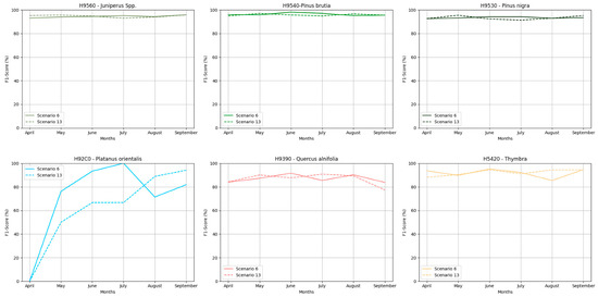
Figure 3.
F1 score performance for each class through Datasets 6 and 13 for Troodos NATURA2000 region.
Based on Figure 4 in the Paphos NATURA2000 region, nearly all habitats again achieved very high F1 score values across all monthly composites and both datasets, ranging from 84.43 to 96.8% with the exceptions of habitats H92D0 and H92C0, which in some cases showed moderate F1 score values, such as for habitat H92D0 in Dataset 13 using the April image composite achieving an F1 score of 78%, while H92C0 achieved 66.6%. Consequently, for this study area, the September image composite was selected based on Dataset 13 for the forest habitats mapping. This selection was due to the composite’s high F1 scores for problematic classes and, apart from that, presented the highest sum of the f-score values from each habitat.
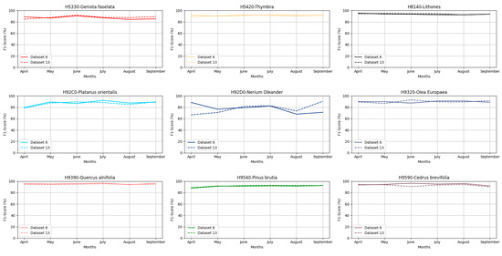
Figure 4.
F1 score performance for each class through Datasets 6 and 13 for the Paphos NATURA2000 region.
Similar to the findings in the other two case studies, in the Akamas region, the majority of habitats across both datasets and all monthly composites achieved high F1 scores, especially the habitats H9540, H9560, H5330 and H9320, as shown in Figure 5. Habitats H92C0, H9290 and H9320 also achieved good accuracies with F1 values ranging from 72 to 89%. In contrast, the problematic class in this case study was H92D0, which presents low F1 score values ranging from 0% to 57%. Following the same approach as with the other two NATURA2000 regions, the June image composite was selected based on Dataset 6.
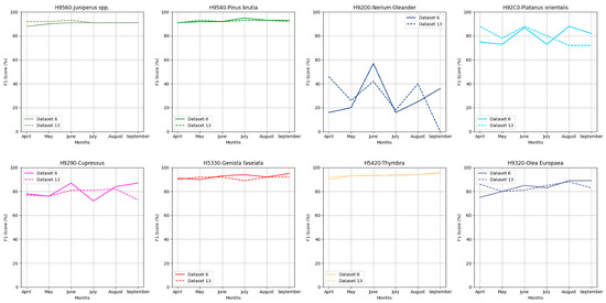
Figure 5.
F1 score performance for each class through Datasets 6 and 13 for Akamas NATURA2000 region.
3.3. Spatial Distribution of Forest Habitats
It is highlighted that Datasets 6 and 13 achieved the highest kappa and OA values, presenting slight differences in their performance. Nevertheless, for the forest habitats mapping, the study also considered the F1 scores across different monthly composites to determine the month with the best performance, especially for the problematic classes. Based on this approach, Dataset 6, utilising the June image composite, was selected for the Troodos and Akamas areas. For the Paphos area, Dataset 13, based on the September image composite, was chosen. The distribution of the habitats across the three case studies is presented in Figure 6.
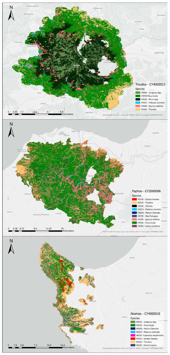
Figure 6.
Distribution of the habitats across the three NATURA2000 regions, Troodos, Paphos and Akamas (arranged from top to bottom).
The evaluation of the area covered by each habitat is presented in Appendix A in Figure A1. Specifically, in the Troodos region, most of the area consisted of H9540 (38.85 km2, 39%) followed by H9530 (31.32 km2, 31%). Furthermore, H9560 covers 12% of the area, and H5420 and H9390 present similar distributions covering 9% and 8%, respectively. The H92C0 has the smallest percentage in this study area, covering 1% of the total area. In Paphos, most of the area consists of H9540 (315.62 km2, 53%), followed by H5420 (119.88 km2, 20%). The habitat H92D0 covers a small area (0.96 km2). Also, 10% of the area comprises H9390 habitat, and H8140, H5330, H9320 and H9590 cover the rest. Furthermore, in the Akamas region, Figure 6 shows most of the area consists of H5420 (48.69 km2, 40%), followed by H9560 (41.35 km2, 34%). In this case, H9540 covers only 12% of the area, contrasting with Paphos and Troodos, where this habitat is dominant. The H5330 and the H9320 present an equal distribution (7%). The habitats H92D0, H92C0 and H9290 cover a very small area of 0.03 km2, 0.4 km2 and 0.46 km2.
4. Discussion
The continuous monitoring of forests worldwide is facilitated using remote sensing techniques that provide information on forest cover, forest habitat distribution and forest health. Focusing on forest habitat identification is vital; for example, conservationists can develop targeted strategies for protecting and recovering specific habitats, particularly species at risk of extinction, by knowing the habitats present in forests [94]. Furthermore, it is an essential tool for mitigating the impact of climate change on forests. This work assessed the potential of integrating Sentinel-1 Sentinel-2 data to improve forest habitat classification. Specifically, the study combined VV and VH backscatter, spectral indices from S1 and S2 bands, spectral indices from S2 and topographical features. The study aimed to identify the most critical inputs for enhancing accuracy using the Random Forest classifier implemented through the GEE for the forest habitats classification in three NATURA2000 regions in Cyprus.
The use of S2 provided better results in contrast with S1 in all datasets. The classification based only on S1 data (Dataset 7 and 9) did not achieve the same high accuracy as the classification with either combined S2 image data; this was also confirmed by [95,96]. It is important to highlight that, in cases where S1 data were combined with topographical features (Dataset 8 and 10), the accuracy was improved but did not achieve the accuracy as the classification was based on combinations of S2 data.
Furthermore, the results find that using NIR, SWIR and Red Edge bands and their combination increases classifier accuracy. These bands are essential since they provide helpful information for discriminating forest habitats. For example, these bands have high sensitivity to the biophysical and biochemical properties of vegetation and can provide helpful information about leaf properties like canopy structure, chlorophyll, etc. [97,98,99]. Based on the results, the use of spectral indices does not significantly increase the classifier’s performance, which is confirmed by Chatziantoniou et al. [100] and Valdivieso-Ros et al. [101]. However, the accuracy was increased when the topographical features were combined. The findings of the study indicate that the topographical features improved the performance of the RF based on the different datasets, which was confirmed by other studies. Specifically, several studies confirm that the use of topographical features such as the elevation, the slope and the aspect improved the classification performance [102,103,104] because the same habitat may present different phenology in different environments, and as a result, present differences in their spectral characteristics [105]. In contrast, the lowest performance occurs when Random Forest relies solely on the Sentinel-1 dataset, aligning with the findings of Lechner et al. [95].
The Random Forest classifier identified most of the forest habitats in the three case studies through all datasets; however, this study identified that H92D0 is a problematic habitat. Based on the results, this habitat achieved low f-score values and, in some datasets, presented complete misclassification (e.g., Dataset 9 in the Paphos region) mainly due to their low proportion in the study area.
Also, based on the monthly composites, the April to September months for 2022 were selected because a large amount of cloud-free data are available in contrast with winter months, where only a few cloud-free data are available and apart from that, in the high elevations there is a presence of snow especially in Troodos region. Furthermore, most of the classified habitats present their blooming during this period, as shown in Appendix B in Table 1. During seasonal variations, the leaves of some deciduous trees fall while others turn yellow. This leads to changes in the tree’s reflectance across the different parts of the wavelength. Furthermore, the reflectance might also be influenced by understory vegetation [106] because the understory vegetation might present a different spectral response than the canopy leaves [107]. Therefore, it is essential to identify the month the classifier achieves its highest performance. Using Dataset 13, which was selected for mapping the forest habitats in the three case studies, the Troodos region was selected for the May monthly composite and the Paphos and Akamas for the June monthly composite.
The study concludes that the Sentinel-2 data can be used solely for this forest habitats classification, but the Sentinel-1 SAR data and the topographical features can improve the classification accuracy. Also, to successfully classify forest habitats, it is essential to collect enough training and validation samples for each class [105] and carefully select appropriate input variables from various data sources such as remotely sensed data, ancillary data, etc.
5. Conclusions
This study aimed to explore integrating Earth observation data with machine learning algorithms for forest habitat classification in NATURA2000 regions in Cyprus. This study is among the first to investigate the combined use of Sentinel-1 and Sentinel-2 data with topographical features through the GEE for forest habitat classification according to the EU Habitat’s Directive in Cyprus. The findings of the study show that the use of Sentinel-2 is significantly more successful than those which rely solely on Sentinel-1 data. Furthermore, the results show that the ideal dataset was Dataset 13, which combines the S1, S2, spectral indices and topographical features. The use of topographical features dramatically improved the performance of the RF.
Furthermore, the results show that the Troodos and Paphos regions are mainly covered by Pinus brutia (H9540), Cyprus’s primary and most important habitats. In contrast, the Akamas region is covered by a small percentage of Pinus brutia (H9540) but is covered mainly by the Phrygana of the Eastern Mediterranean (H5420) and Juniperus spp. (H9560). In addition, the study presented some difficulties in classifying riverside shrub (H92D0) habitats and, in some datasets, presented total misclassification. The study concludes that the use of remote sensing is a fundamental tool for forest habitat classification, especially in NATURA2000 regions. The European Commission require a report on the status of NATURA2000 habitats every six years and the use of remote sensing data, such as satellite imagery, has proven to be the most effective way of assessing and monitoring environmental changes. Therefore, the methodology used in this study provides the ability for future use in monitoring environmental changes in Cyprus’s Troodos, Paphos and Akamas NATURA2000 regions. With additional habitat samples and the computational power of GEE, this approach can be extended to other NATURA sites in Cyprus.
Author Contributions
Conceptualisation, M.P.; methodology, M.P. and C.T.; software, M.P., C.T. and F.E.; validation, K.P. and C.D. (Constantinos Dimitrakopoulos); formal analysis, M.P.; investigation, M.P., C.T. and F.E.; resources, K.P. and C.D. (Constantinos Dimitrakopoulos); data curation, K.P., C.D. (Constantinos Dimitrakopoulos), M.P., C.T. and F.E.; writing—original draft preparation, M.P., C.T., F.E. and I.Z.G.; writing—review and editing, M.P., C.T., I.Z.G., K.T., C.D (Chris Danezis). and D.H.; visualisation, M.P.; supervision, K.T. and D.H.; project administration, D.H.; funding acquisition, D.H. All authors have read and agreed to the published version of the manuscript.
Funding
This work was funded through the EXCELSIOR Teaming project (Grant Agreement No. 857510, www.excelsior2020.eu, accessed on 9 March 2024) that has received funding from the European Union’s Horizon 2020 research and innovation programme and from the Government of the Republic of Cyprus through the Directorate General for the European Programmes, Coordination and Development.
Data Availability Statement
Data are contained within the article.
Acknowledgments
The authors acknowledge the “EXCELSIOR”: ERATOSTHENES: Excellence Research Centre for Earth Surveillance and Space-Based Monitoring of the Environment H2020 Widespread Teaming project (www.excelsior2020.eu, accessed on 9 March 2024). The “EXCELSIOR” project has received funding from the European Union’s Horizon 2020 research and innovation programme under Grant Agreement No. 857510, from the Government of the Republic of Cyprus through the Directorate General for the European Programmes, Coordination and Development and the Cyprus University of Technology. The authors would also like to thank the Forest Department of the Ministry of Agriculture, Rural Development and Environment of the Republic of Cyprus for the provision of the in situ data, which are collected in the framework of LIFE IP Physis—Managing the Natura 2000 network in Cyprus and shaping a sustainable future.
Conflicts of Interest
The authors declare no conflicts of interest.
Appendix A
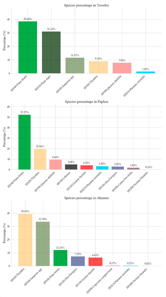
Figure A1.
Evaluation of the area covered by each habitat across the three case studies, respectively.
Appendix B
Table A1.
Habitats that are classified in the three case studies and the corresponding blooming months (indicated by the symbol  ).
).
).
Table A1.
Habitats that are classified in the three case studies and the corresponding blooming months (indicated by the symbol ).
).| Habitat | Habitat Type | Deciduous/Evergreens | Months of the Year | ||||||||||||
|---|---|---|---|---|---|---|---|---|---|---|---|---|---|---|---|
| 1 | 2 | 3 | 4 | 5 | 6 | 7 | 8 | 9 | 10 | 11 | 12 | ||||
| H5330 | Thermo-Mediterranean pre-steppe scrub with | Genista fasselata | Deciduous | | | | | ||||||||
| H5420 | Phrygana of the eastern Mediterranean | Thymbra capitata | - | | | | | | | ||||||
| Sarcopoterium spinosum | | | | ||||||||||||
| Cistus sp. | | | | | |||||||||||
| H8140 | Eastern Mediterranean moraine | - | - | - | - | - | - | - | - | - | - | - | - | - | |
| H92C0 | Eastern sycamore riparian forests | Platanus orientalis | Deciduous (November to March without foliage) | | | ||||||||||
| Alnus orientalis | | | | | |||||||||||
| H92D0 | Riverside Shrubs | Nerium oleander | Deciduous | | | | |||||||||
| Tamarix sp. | Deciduous | | | | |||||||||||
| Vitex agnus-castus | Evergreens | | | | | | | ||||||||
| H9320 | Evergreen sclerophyll shrubs | Olea europaea | Deciduous | | | | |||||||||
| Ceratonia siliqua | Deciduous | | | | |||||||||||
| Pistacia lentiscus | Deciduous | | | ||||||||||||
| H9390 | Shrubs of Quercus alnifolia | Quercus alnifolia | Deciduous | | | ||||||||||
| H9540 | Pinus brutia Forest | Pinus brutia | Evergreens | | | | |||||||||
| H9590 | Cedrus brevifolia Forest | Cedrus brevifolia | Deciduous | | | ||||||||||
| H9560 | Juniperus spp. Forest | J. foeditissima | Evergreens | | | | | | | | |||||
| J. excelsa | Evergreens | | | | | | | | |||||||
| J. phoenicea | Evergreens | | | | |||||||||||
| J. oxycedrus | Evergreens | | | ||||||||||||
| H9530 | Pinus nigra Forest | Pinus nigra | Evergreens | | | ||||||||||
| H9290 | Cupressus Forest | Cupressus sempervirens | Deciduous | | | | |||||||||
References
- Fassnacht, F.E.; Latifi, H.; Stereńczak, K.; Modzelewska, A.; Lefsky, M.; Waser, L.T.; Straub, C.; Ghosh, A. Review of Studies on Tree Species Classification from Remotely Sensed Data. Remote Sens. Environ. 2016, 186, 64–87. [Google Scholar] [CrossRef]
- Spurr, S.H. Aerial Photographs in Forestry; Ronald Press Company: New York, NY, USA, 1948. [Google Scholar]
- Wan, H.; Tang, Y.; Jing, L.; Li, H.; Qiu, F.; Wu, W. Tree Species Classification of Forest Stands Using Multisource Remote Sensing Data. Remote Sens. 2021, 13, 144. [Google Scholar] [CrossRef]
- Prodromou, M.; Gitas, I.; Themistocleous, K.; Nisantzi, A.; Mamouri, R.-E.; Ene, D.; Danezis, C.; Bühl, J.; Hadjimitsis, D. The Use of Remote Sensing Data for the Fire Damage Assessment in a Burnt Area in Cyprus. In Proceedings of the Ninth International Conference on Remote Sensing and Geoinformation of the Environment (RSCy2023), Ayia Napa, Cyprus, 3–5 April 2023; Volume 12786, p. 1278608. [Google Scholar]
- Theocharidis, C.; Gitas, I.; Danezis, C.; Hadjimitsis, D. Satellite Times-Series Analysis and Assessment of the BFAST Algorithm to Detect Possible Abrupt Changes in Forest Seasonality Utilising Sentinel-1 and Sentinel-2 Data. Case Study: Paphos Forest, Cyprus. In Proceedings of the EGU General Assembly 2023, Vienna, Austria, 24–28 April 2023. [Google Scholar]
- Prodromou, M.; Gitas, I.; Themistocleous, K.; Hadjimitsis, D. The Implementation of the Forest Canopy Density (FCD) Model for Coniferous Ecosystems in Cyprus Forests, Using Landsat-8 and Sentinel-2 Satellite Data. In Proceedings of the EGU General Assembly Conference Abstracts, Vienna, Austria, 3–8 April 2022; p. EGU2219865. [Google Scholar]
- European Commission. The Natura 2000 Protected Areas Network 2018. Available online: https://ec.europa.eu/environment/nature/natura2000/ (accessed on 30 November 2023).
- Pandoteira. What Is Natura 2000? Available online: https://pandoteira.cy/what-is-natura-2000/# (accessed on 2 October 2023).
- Tsintides, T.; Christodoulou, C.S.; Delipetrou, P.; Georghiou, K. The Red Data Book of the Flora of Cyprus; Cyprus Forestry Association: Lefkosia, Cyprus, 2007; Volume 465. [Google Scholar]
- Nila, M.U.S.; Beierkuhnlein, C.; Jaeschke, A.; Hoffmann, S.; Hossain, M.L. Predicting the Effectiveness of Protected Areas of Natura 2000 under Climate Change. Ecol. Process. 2019, 8, 13. [Google Scholar] [CrossRef]
- Ma, M.; Liu, J.; Liu, M.; Zeng, J.; Li, Y. Tree Species Classification Based on Sentinel-2 Imagery and Random Forest Classifier in the Eastern Regions of the Qilian Mountains. Forests 2021, 12, 1736. [Google Scholar] [CrossRef]
- Immitzer, M.; Atzberger, C.; Koukal, T. Tree Species Classification with Random Forest Using Very High Spatial Resolution 8-Band WorldView-2 Satellite Data. Remote Sens. 2012, 4, 2661–2693. [Google Scholar] [CrossRef]
- Tariq, A.; Jiango, Y.; Li, Q.; Gao, J.; Lu, L.; Soufan, W.; Almutairi, K.F.; Habib-ur-Rahman, M. Modelling, Mapping and Monitoring of Forest Cover Changes, Using Support Vector Machine, Kernel Logistic Regression and Naive Bayes Tree Models with Optical Remote Sensing Data. Heliyon 2023, 9, e13212. [Google Scholar] [CrossRef] [PubMed]
- Cengiz, A.; Budak, M.; Yağmur, N.; Balçik, F. Comparison between Random Forest and Support Vector Machine Algorithms for LULC Classification. Int. J. Eng. Geosci. 2023, 8, 1–10. [Google Scholar]
- Zagajewski, B.; Kluczek, M.; Raczko, E.; Njegovec, A.; Dabija, A.; Kycko, M. Comparison of Random Forest, Support Vector Machines, and Neural Networks for Post-Disaster Forest Species Mapping of the Krkonoše/Karkonosze Transboundary Biosphere Reserve. Remote Sens. 2021, 13, 2581. [Google Scholar] [CrossRef]
- Raczko, E.; Zagajewski, B. Comparison of Support Vector Machine, Random Forest and Neural Network Classifiers for Tree Species Classification on Airborne Hyperspectral APEX Images. Eur. J. Remote Sens. 2017, 50, 144–154. [Google Scholar] [CrossRef]
- Knauer, U.; von Rekowski, C.S.; Stecklina, M.; Krokotsch, T.; Pham Minh, T.; Hauffe, V.; Kilias, D.; Ehrhardt, I.; Sagischewski, H.; Chmara, S. Tree Species Classification Based on Hybrid Ensembles of a Convolutional Neural Network (CNN) and Random Forest Classifiers. Remote Sens. 2019, 11, 2788. [Google Scholar] [CrossRef]
- Zhang, B.; Zhao, L.; Zhang, X. Three-Dimensional Convolutional Neural Network Model for Tree Species Classification Using Airborne Hyperspectral Images. Remote Sens. Environ. 2020, 247, 111938. [Google Scholar] [CrossRef]
- Xi, Y.; Ren, C.; Tian, Q.; Ren, Y.; Dong, X.; Zhang, Z. Exploitation of Time Series Sentinel-2 Data and Different Machine Learning Algorithms for Detailed Tree Species Classification. IEEE J. Sel. Top. Appl. Earth Obs. Remote Sens. 2021, 14, 7589–7603. [Google Scholar] [CrossRef]
- Reuß, F.; Greimeister-Pfeil, I.; Vreugdenhil, M.; Wagner, W. Comparison of Long Short-Term Memory Networks and Random Forest for Sentinel-1 Time Series Based Large Scale Crop Classification. Remote Sens. 2021, 13, 5000. [Google Scholar] [CrossRef]
- He, T.; Zhou, H.; Xu, C.; Hu, J.; Xue, X.; Xu, L.; Lou, X.; Zeng, K.; Wang, Q. Deep Learning in Forest Tree Species Classification Using Sentinel-2 on Google Earth Engine: A Case Study of Qingyuan County. Sustainability 2023, 15, 2741. [Google Scholar] [CrossRef]
- Chang, T.; Rasmussen, B.; Dickson, B.; Zachmann, L. Chimera: A Multi-Task Recurrent Convolutional Neural Network for Forest Classification and Structural Estimation. Remote Sens. 2019, 11, 768. [Google Scholar] [CrossRef]
- Sumsion, G.R.; Bradshaw, M.S.; Hill, K.T.; Pinto, L.D.G.; Piccolo, S.R. Remote Sensing Tree Classification with a Multilayer Perceptron. PeerJ 2019, 7, e6101. [Google Scholar] [CrossRef] [PubMed]
- Tsai, Y.; Stow, D.; Chen, H.; Lewison, R.; An, L.; Shi, L. Mapping Vegetation and Land Use Types in Fanjingshan National Nature Reserve Using Google Earth Engine. Remote Sens. 2018, 10, 927. [Google Scholar] [CrossRef]
- Aji, M.A.P.; Kamal, M.; Farda, N.M. Mangrove Species Mapping through Phenological Analysis Using Random Forest Algorithm on Google Earth Engine. Remote Sens. Appl. 2023, 30, 100978. [Google Scholar] [CrossRef]
- Bessinger, M.; Lück-Vogel, M.; Skowno, A.; Conrad, F. Landsat-8 Based Coastal Ecosystem Mapping in South Africa Using Random Forest Classification in Google Earth Engine. S. Afr. J. Bot. 2022, 150, 928–939. [Google Scholar] [CrossRef]
- Teluguntla, P.; Thenkabail, P.S.; Oliphant, A.; Xiong, J.; Gumma, M.K.; Congalton, R.G.; Yadav, K.; Huete, A. A 30-m Landsat-Derived Cropland Extent Product of Australia and China Using Random Forest Machine Learning Algorithm on Google Earth Engine Cloud Computing Platform. ISPRS J. Photogramm. Remote Sens. 2018, 144, 325–340. [Google Scholar] [CrossRef]
- Magidi, J.; Nhamo, L.; Mpandeli, S.; Mabhaudhi, T. Application of the Random Forest Classifier to Map Irrigated Areas Using Google Earth Engine. Remote Sens. 2021, 13, 876. [Google Scholar] [CrossRef]
- Phan, T.N.; Kuch, V.; Lehnert, L.W. Land Cover Classification Using Google Earth Engine and Random Forest Classifier—The Role of Image Composition. Remote Sens. 2020, 12, 2411. [Google Scholar] [CrossRef]
- Antoniadis, K.; Georgopoulos, N.; Katagis, T.; Stavrakoudis, D.; Gitas, I.Z. Classification of Seasonal Sentinel-2 Imagery for Mapping Vegetation in Mediterranean Ecosystems. In Proceedings of the Ninth International Conference on Remote Sensing and Geoinformation of the Environment (RSCy2023), Ayia Napa, Cyprus, 3–5 April 2023; p. 12. [Google Scholar]
- Abdel-Rahman, E.M.; Mutanga, O.; Adam, E.; Ismail, R. Detecting Sirex Noctilio Grey-Attacked and Lightning-Struck Pine Trees Using Airborne Hyperspectral Data, Random Forest and Support Vector Machines Classifiers. ISPRS J. Photogramm. Remote Sens. 2014, 88, 48–59. [Google Scholar] [CrossRef]
- Rodriguez-Galiano, V.F.; Chica-Rivas, M. Evaluation of Different Machine Learning Methods for Land Cover Mapping of a Mediterranean Area Using Multi-Seasonal Landsat Images and Digital Terrain Models. Int. J. Digit. Earth 2014, 7, 492–509. [Google Scholar] [CrossRef]
- Belgiu, M.; Drăguţ, L. Random Forest in Remote Sensing: A Review of Applications and Future Directions. ISPRS J. Photogramm. Remote Sens. 2016, 114, 24–31. [Google Scholar] [CrossRef]
- van Beijma, S.; Comber, A.; Lamb, A. Random Forest Classification of Salt Marsh Vegetation Habitats Using Quad-Polarimetric Airborne SAR, Elevation and Optical RS Data. Remote Sens. Environ. 2014, 149, 118–129. [Google Scholar] [CrossRef]
- Wang, Z.; Ma, Y.; Zhang, Y.; Shang, J. Review of Remote Sensing Applications in Grassland Monitoring. Remote Sens. 2022, 14, 2903. [Google Scholar] [CrossRef]
- Yuan, Y.; Wen, Q.; Zhao, X.; Liu, S.; Zhu, K.; Hu, B. Identifying Grassland Distribution in a Mountainous Region in Southwest China Using Multi-Source Remote Sensing Images. Remote Sens. 2022, 14, 1472. [Google Scholar] [CrossRef]
- Carbonell-Rivera, J.P.; Torralba, J.; Estornell, J.; Ruiz, L.Á.; Crespo-Peremarch, P. Classification of Mediterranean Shrub Species from UAV Point Clouds. Remote Sens. 2022, 14, 199. [Google Scholar] [CrossRef]
- Detka, J.; Coyle, H.; Gomez, M.; Gilbert, G.S. A Drone-Powered Deep Learning Methodology for High Precision Remote Sensing in California’s Coastal Shrubs. Drones 2023, 7, 421. [Google Scholar] [CrossRef]
- Wang, X.; Tan, L.; Fan, J. Performance Evaluation of Mangrove Species Classification Based on Multi-Source Remote Sensing Data Using Extremely Randomized Trees in Fucheng Town, Leizhou City, Guangdong Province. Remote Sens. 2023, 15, 1386. [Google Scholar] [CrossRef]
- Lassalle, G.; Ferreira, M.P.; La Rosa, L.E.C.; Scafutto, R.D.M.; de Souza Filho, C.R. Advances in Multi-and Hyperspectral Remote Sensing of Mangrove Species: A Synthesis and Study Case on Airborne and Multisource Spaceborne Imagery. ISPRS J. Photogramm. Remote Sens. 2023, 195, 298–312. [Google Scholar] [CrossRef]
- Mahdavi, S.; Salehi, B.; Granger, J.; Amani, M.; Brisco, B.; Huang, W. Remote Sensing for Wetland Classification: A Comprehensive Review. GIScience Remote Sens. 2018, 55, 623–658. [Google Scholar] [CrossRef]
- Tiner, R.W.; Lang, M.W.; Klemas, V.V. (Eds.) Remote Sensing of Wetlands; CRC Press: Boca Raton, FL, USA, 2015; ISBN 9781482237382. [Google Scholar]
- Tariq, A.; Yan, J.; Gagnon, A.S.; Riaz Khan, M.; Mumtaz, F. Mapping of Cropland, Cropping Patterns and Crop Types by Combining Optical Remote Sensing Images with Decision Tree Classifier and Random Forest. Geo-Spat. Inf. Sci. 2023, 26, 302–320. [Google Scholar] [CrossRef]
- Davidson, S.; Santos, M.; Sloan, V.; Watts, J.; Phoenix, G.; Oechel, W.; Zona, D. Mapping Arctic Tundra Vegetation Communities Using Field Spectroscopy and Multispectral Satellite Data in North Alaska, USA. Remote Sens. 2016, 8, 978. [Google Scholar] [CrossRef]
- Tzirkalli, E.; Eliades, E.; Chrysopolitou, V.; Hatziiordanou, L.; Panagiotou, N.; Agapiou, A.; Antoniou, A.; Xenophontos, M.; Panayiotou, C.; Hadjicharalambous, H. Natura 2000 Habitat Mapping in Cyprus Using High Resolution Orthophoto Maps. In Proceedings of the Sixth International Conference on Remote Sensing and Geoinformation of the Environment (RSCy2018), Paphos, Cyprus, 26–29 March 2018; Volume 10773, pp. 484–492. [Google Scholar]
- Mutanga, O.; Kumar, L. Google Earth Engine Applications. Remote Sens. 2019, 11, 591. [Google Scholar] [CrossRef]
- Kaplan, G. Broad-Leaved and Coniferous Forest Classification in Google Earth Engine Using Sentinel Imagery. In Proceedings of the 1st International Electronic Conference on Forests—Forests for a Better Future: Sustainability, Innovation, Interdisciplinarity, Virtual, 15–30 November 2020; MDPI: Basel, Switzerland, 2020; p. 64. [Google Scholar]
- Praticò, S.; Solano, F.; Di Fazio, S.; Modica, G. Machine Learning Classification of Mediterranean Forest Habitats in Google Earth Engine Based on Seasonal Sentinel-2 Time-Series and Input Image Composition Optimisation. Remote Sens. 2021, 13, 586. [Google Scholar] [CrossRef]
- Kamal, M.; Jamaluddin, I.; Parela, A.; Farda, N.M. Comparison of Google Earth Engine (GEE)-Based Machine Learning Classifiers for Mangrove Mapping. In Proceedings of the 40th Asian Conference Remote Sensing, ACRS, Daejeon, Republic of Korea, 14–18 October 2019; pp. 1–8. [Google Scholar]
- Marcinkowska-Ochtyra, A.; Ochtyra, A.; Raczko, E.; Kopeć, D. Natura 2000 Grassland Habitats Mapping Based on Spectro-Temporal Dimension of Sentinel-2 Images with Machine Learning. Remote Sens. 2023, 15, 1388. [Google Scholar] [CrossRef]
- Feilhauer, H.; Dahlke, C.; Doktor, D.; Lausch, A.; Schmidtlein, S.; Schulz, G.; Stenzel, S. Mapping the Local Variability of Natura 2000 Habitats with Remote Sensing. Appl. Veg. Sci. 2014, 17, 765–779. [Google Scholar] [CrossRef]
- Santoro, A.; Piras, F.; Fiore, B.; Bazzurro, A.; Agnoletti, M. Forest-Cover Changes in European Natura 2000 Sites in the Period 2012–2018. Forests 2024, 15, 232. [Google Scholar] [CrossRef]
- KopeĿ, D.; Michalska-Hejduk, D.; Sſawik, S.; Berezowski, T.; Borowski, M.; Rosadziſski, S.; Chormaſski, J. Application of Multisensoral Remote Sensing Data in the Mapping of Alkaline Fens Natura 2000 Habitat. Ecol. Indic. 2016, 70, 196–208. [Google Scholar] [CrossRef]
- Alexandridis, T.K.; Lazaridou, E.; Tsirika, A.; Zalidis, G.C. Using Earth Observation to Update a Natura 2000 Habitat Map for a Wetland in Greece. J. Environ. Manag. 2009, 90, 2243–2251. [Google Scholar] [CrossRef] [PubMed]
- Sittaro, F.; Hutengs, C.; Semella, S.; Vohland, M. A Machine Learning Framework for the Classification of Natura 2000 Habitat Types at Large Spatial Scales Using MODIS Surface Reflectance Data. Remote Sens. 2022, 14, 823. [Google Scholar] [CrossRef]
- Marcinkowska-Ochtyra, A.; Gryguc, K.; Ochtyra, A.; Kopeć, D.; Jarocińska, A.; Sławik, Ł. Multitemporal Hyperspectral Data Fusion with Topographic Indices—Improving Classification of Natura 2000 Grassland Habitats. Remote Sens. 2019, 11, 2264. [Google Scholar] [CrossRef]
- Čahojová, L.; Ambroz, M.; Jarolímek, I.; Kollár, M.; Mikula, K.; Šibík, J.; Šibíková, M. Exploring Natura 2000 Habitats by Satellite Image Segmentation Combined with Phytosociological Data: A Case Study from the Čierny Balog Area (Central Slovakia). Sci. Rep. 2022, 12, 18375. [Google Scholar] [CrossRef] [PubMed]
- Hadjimitsis, D.G.; Themistokleous, K.; Onoufriou, T. Environmental Monitoring of Spatial Data for the Application of NATURA 2000 Network in Cyprus Using Remote Sensing and GIS. In Proceedings of the International Conference ’PRE9: Protection and Restoration of the Environment, Kefalonia, Greece, 30 June–3 July 2008. [Google Scholar]
- European Environment Agency. Natura 2000, Standard Data form Site CY2000006. Available online: https://natura2000.eea.europa.eu/Natura2000/SDF.aspx?site=CY2000006 (accessed on 30 November 2023).
- European Environment Agency. Natura 2000, Standard Data form Site CY4000010. Available online: https://natura2000.eea.europa.eu/Natura2000/SDF.aspx?site=CY4000010 (accessed on 30 November 2023).
- European Environment Agency. Natura 2000, Standard Data form Site CY5000004. Available online: https://natura2000.eea.europa.eu/Natura2000/SDF.aspx?site=CY5000004 (accessed on 30 November 2023).
- Schubert, A.; Miranda, N.; Geudtner, D.; Small, D. Sentinel-1A/B Combined Product Geolocation Accuracy. Remote Sens. 2017, 9, 607. [Google Scholar] [CrossRef]
- Geudtner, D.; Torres, R.; Snoeij, P.; Davidson, M.; Rommen, B. Sentinel-1 System Capabilities and Applications. In Proceedings of the 2014 IEEE Geoscience and Remote Sensing Symposium, Quebec City, QC, Canada, 13–18 July 2014; pp. 1457–1460. [Google Scholar]
- European Space Agency. Mission Ends for Copernicus Sentinel-1B Satellite. Available online: https://www.esa.int/Applications/Observing_the_Earth/Copernicus/Sentinel-1/Mission_ends_for_Copernicus_Sentinel-1B_satellite (accessed on 30 November 2023).
- Spoto, F.; Sy, O.; Laberinti, P.; Martimort, P.; Fernandez, V.; Colin, O.; Hoersch, B.; Meygret, A. Overview of Sentinel-2. In Proceedings of the 2012 IEEE International Geoscience and Remote Sensing Symposium, Munich, Germany, 22–27 July 2012; pp. 1707–1710. [Google Scholar]
- Drusch, M.; Del Bello, U.; Carlier, S.; Colin, O.; Fernandez, V.; Gascon, F.; Hoersch, B.; Isola, C.; Laberinti, P.; Martimort, P.; et al. Sentinel-2: ESA’s Optical High-Resolution Mission for GMES Operational Services. Remote Sens. Environ. 2012, 120, 25–36. [Google Scholar] [CrossRef]
- Xia, J.; Yokoya, N.; Pham, T.D. Probabilistic Mangrove Species Mapping with Multiple-Source Remote-Sensing Datasets Using Label Distribution Learning in Xuan Thuy National Park, Vietnam. Remote Sens. 2020, 12, 3834. [Google Scholar] [CrossRef]
- Mahdavi, S.; Salehi, B.; Amani, M.; Granger, J.; Brisco, B.; Huang, W. A Dynamic Classification Scheme for Mapping Spectrally Similar Classes: Application to Wetland Classification. Int. J. Appl. Earth Obs. Geoinf. 2019, 83, 101914. [Google Scholar] [CrossRef]
- Ghorbanian, A.; Zaghian, S.; Asiyabi, R.M.; Amani, M.; Mohammadzadeh, A.; Jamali, S. Mangrove Ecosystem Mapping Using Sentinel-1 and Sentinel-2 Satellite Images and Random Forest Algorithm in Google Earth Engine. Remote Sens. 2021, 13, 2565. [Google Scholar] [CrossRef]
- Kpienbaareh, D.; Sun, X.; Wang, J.; Luginaah, I.; Bezner Kerr, R.; Lupafya, E.; Dakishoni, L. Crop Type and Land Cover Mapping in Northern Malawi Using the Integration of Sentinel-1, Sentinel-2, and PlanetScope Satellite Data. Remote Sens. 2021, 13, 700. [Google Scholar] [CrossRef]
- De Luca, G.; Silva, M.N.J.; Di Fazio, S.; Modica, G. Integrated Use of Sentinel-1 and Sentinel-2 Data and Open-Source Machine Learning Algorithms for Land Cover Mapping in a Mediterranean Region. Eur. J. Remote Sens. 2022, 55, 52–70. [Google Scholar] [CrossRef]
- Nasiri, V.; Beloiu, M.; Asghar Darvishsefat, A.; Griess, V.C.; Maftei, C.; Waser, L.T. Mapping Tree Species Composition in a Caspian Temperate Mixed Forest Based on Spectral-Temporal Metrics and Machine Learning. Int. J. Appl. Earth Obs. Geoinf. 2023, 116, 103154. [Google Scholar] [CrossRef]
- Papachristoforou, A.; Prodromou, M.; Hadjimitsis, D.; Christoforou, M. Detecting and Distinguishing between Apicultural Plants Using UAV Multispectral Imaging. PeerJ 2023, 11, e15065. [Google Scholar] [CrossRef]
- Tucker, C.J. Red and Photographic Infrared Linear Combinations for Monitoring Vegetation. Remote Sens. Environ. 1979, 8, 127–150. [Google Scholar] [CrossRef]
- Huntjr, E.; Rock, B. Detection of Changes in Leaf Water Content Using Near- and Middle-Infrared Reflectances. Remote Sens. Environ. 1989, 30, 43–54. [Google Scholar] [CrossRef]
- Barnes, E.M.; Clarke, T.R.; Richards, S.E.; Colaizzi, P.D.; Haberland, J.; Kostrzewski, M.; Waller, P.; Choi, C.; Riley, E.; Thompson, T.; et al. Coincident Detection of Crop Water Stress, Nitrogen Status and Canopy Density Using Ground Based Multispectral Data. In Proceedings of the Fifth International Conference on Precision Agriculture, Bloomington, MN, USA, 16–19 July 2000. [Google Scholar]
- Kumar, D.; Rao, S.; Sharma, J.R. Radar Vegetation Index as an Alternative to NDVI for Monitoring of Soyabean and Cotton. In Proceedings of the XXXIII INCA International Congress (Indian Cartographer), Jodhpur, India, 19–21 September 2013; pp. 91–96. [Google Scholar]
- Jain, S.; Batra, K.U.; Mishra, P. Land Cover Classification by Decision Based Classifier Using Dual Polarimetric SAR Observables. In Proceedings of the 2022 IEEE 9th Uttar Pradesh Section International Conference on Electrical, Electronics and Computer Engineering (UPCON), Allahabad, India, 2–4 December 2022; pp. 1–6. [Google Scholar]
- Gitelson, A.A.; Gritz, Y.; Merzlyak, M.N. Relationships between Leaf Chlorophyll Content and Spectral Reflectance and Algorithms for Non-Destructive Chlorophyll Assessment in Higher Plant Leaves. J. Plant Physiol. 2003, 160, 271–282. [Google Scholar] [CrossRef]
- Huete, A.; Didan, K.; Miura, T.; Rodriguez, E.P.; Gao, X.; Ferreira, L.G. Overview of the Radiometric and Biophysical Performance of the MODIS Vegetation Indices. Remote Sens. Environ. 2002, 83, 195–213. [Google Scholar] [CrossRef]
- Huete, A.R. A Soil-Adjusted Vegetation Index (SAVI). Remote Sens. Environ. 1988, 25, 295–309. [Google Scholar] [CrossRef]
- Kim, Y.; Jackson, T.; Bindlish, R.; Lee, H.; Hong, S. Radar Vegetation Index for Estimating the Vegetation Water Content of Rice and Soybean. IEEE Geosci. Remote Sens. Lett. 2012, 9, 564–568. [Google Scholar] [CrossRef]
- Mitchard, E.T.A.; Saatchi, S.S.; White, L.J.T.; Abernethy, K.A.; Jeffery, K.J.; Lewis, S.L.; Collins, M.; Lefsky, M.A.; Leal, M.E.; Woodhouse, I.H.; et al. Mapping Tropical Forest Biomass with Radar and Spaceborne LiDAR in Lopé National Park, Gabon: Overcoming Problems of High Biomass and Persistent Cloud. Biogeosciences 2012, 9, 179–191. [Google Scholar] [CrossRef]
- Breiman, L. Random Forests. Mach. Learn. 2001, 45, 5–32. [Google Scholar] [CrossRef]
- Vorpahl, P.; Elsenbeer, H.; Märker, M.; Schröder, B. How Can Statistical Models Help to Determine Driving Factors of Landslides? Ecol. Model. 2012, 239, 27–39. [Google Scholar] [CrossRef]
- Ließ, M.; Glaser, B.; Huwe, B. Uncertainty in the Spatial Prediction of Soil Texture. Geoderma 2012, 170, 70–79. [Google Scholar] [CrossRef]
- Löw, F.; Dimov, D.; Kenjabaev, S.; Zaitov, S.; Stulina, G.; Dukhovny, V. Land Cover Change Detection in the Aralkum with Multi-Source Satellite Datasets. GIsci Remote Sens. 2022, 59, 17–35. [Google Scholar] [CrossRef]
- Zhang, X.; Wu, B.; Ponce-Campos, G.; Zhang, M.; Chang, S.; Tian, F. Mapping Up-to-Date Paddy Rice Extent at 10 M Resolution in China through the Integration of Optical and Synthetic Aperture Radar Images. Remote Sens. 2018, 10, 1200. [Google Scholar] [CrossRef]
- Deines, J.M.; Kendall, A.D.; Crowley, M.A.; Rapp, J.; Cardille, J.A.; Hyndman, D.W. Mapping Three Decades of Annual Irrigation across the US High Plains Aquifer Using Landsat and Google Earth Engine. Remote Sens. Environ. 2019, 233, 111400. [Google Scholar] [CrossRef]
- Zeng, H.; Wu, B.; Wang, S.; Musakwa, W.; Tian, F.; Mashimbye, Z.E.; Poona, N.; Syndey, M. A Synthesizing Land-Cover Classification Method Based on Google Earth Engine: A Case Study in Nzhelele and Levhuvu Catchments, South Africa. Chin. Geogr. Sci. 2020, 30, 397–409. [Google Scholar] [CrossRef]
- Tran, V.A.; Le, T.L.; Nguyen, N.H.; Le, T.N.; Tran, H.H. Monitoring Vegetation Cover Changes by Sentinel-1 Radar Images Using Random Forest Classification Method. Inz. Miner. 2021, 1, 441–452. [Google Scholar] [CrossRef]
- Lu, D.; Weng, Q. A Survey of Image Classification Methods and Techniques for Improving Classification Performance. Int. J. Remote Sens. 2007, 28, 823–870. [Google Scholar] [CrossRef]
- Lee, J.S.H.; Wich, S.; Widayati, A.; Koh, L.P. Detecting Industrial Oil Palm Plantations on Landsat Images with Google Earth Engine. Remote Sens. Appl. 2016, 4, 219–224. [Google Scholar] [CrossRef]
- Vorovencii, I.; Dincă, L.; Crișan, V.; Postolache, R.-G.; Codrean, C.-L.; Cătălin, C.; Greșiță, C.I.; Chima, S.; Gavrilescu, I. Local-Scale Mapping of Tree Species in a Lower Mountain Area Using Sentinel-1 and -2 Multitemporal Images, Vegetation Indices, and Topographic Information. Front. For. Glob. Chang. 2023, 6, 1220253. [Google Scholar] [CrossRef]
- Lechner, M.; Dostálová, A.; Hollaus, M.; Atzberger, C.; Immitzer, M. Combination of Sentinel-1 and Sentinel-2 Data for Tree Species Classification in a Central European Biosphere Reserve. Remote Sens. 2022, 14, 2687. [Google Scholar] [CrossRef]
- Hościło, A.; Lewandowska, A. Mapping Forest Type and Tree Species on a Regional Scale Using Multi-Temporal Sentinel-2 Data. Remote Sens. 2019, 11, 929. [Google Scholar] [CrossRef]
- Mngadi, M.; Odindi, J.; Peerbhay, K.; Mutanga, O. Examining the Effectiveness of Sentinel-1 and 2 Imagery for Commercial Forest Species Mapping. Geocarto Int. 2021, 36, 1–12. [Google Scholar] [CrossRef]
- Sibanda, M.; Mutanga, O.; Rouget, M. Comparing the Spectral Settings of the New Generation Broad and Narrow Band Sensors in Estimating Biomass of Native Grasses Grown under Different Management Practices. GIScience Remote Sens. 2016, 53, 614–633. [Google Scholar] [CrossRef]
- Dube, T.; Mutanga, O. Investigating the Robustness of the New Landsat-8 Operational Land Imager Derived Texture Metrics in Estimating Plantation Forest Aboveground Biomass in Resource Constrained Areas. ISPRS J. Photogramm. Remote Sens. 2015, 108, 12–32. [Google Scholar] [CrossRef]
- Deng, S.; Katoh, M.; Guan, Q.; Yin, N.; Li, M. Interpretation of Forest Resources at the Individual Tree Level at Purple Mountain, Nanjing City, China, Using WorldView-2 Imagery by Combining GPS, RS and GIS Technologies. Remote Sens. 2013, 6, 87–110. [Google Scholar] [CrossRef]
- Valdivieso-Ros, C.; Alonso-Sarria, F.; Gomariz-Castillo, F. Effect of the Synergetic Use of Sentinel-1, Sentinel-2, LiDAR and Derived Data in Land Cover Classification of a Semiarid Mediterranean Area Using Machine Learning Algorithms. Remote Sens. 2023, 15, 312. [Google Scholar] [CrossRef]
- Waśniewski, A.; Hościło, A.; Aune-Lundberg, L. The Impact of Selection of Reference Samples and DEM on the Accuracy of Land Cover Classification Based on Sentinel-2 Data. Remote Sens. Appl. 2023, 32, 101035. [Google Scholar] [CrossRef]
- Polykretis, C.; Grillakis, M.; Alexakis, D. Exploring the Impact of Various Spectral Indices on Land Cover Change Detection Using Change Vector Analysis: A Case Study of Crete Island, Greece. Remote Sens. 2020, 12, 319. [Google Scholar] [CrossRef]
- Yu, X.; Lu, D.; Jiang, X.; Li, G.; Chen, Y.; Li, D.; Chen, E. Examining the Roles of Spectral, Spatial, and Topographic Features in Improving Land-Cover and Forest Classifications in a Subtropical Region. Remote Sens. 2020, 12, 2907. [Google Scholar] [CrossRef]
- Liu, X.; Frey, J.; Munteanu, C.; Still, N.; Koch, B. Mapping Tree Species Diversity in Temperate Montane Forests Using Sentinel-1 and Sentinel-2 Imagery and Topography Data. Remote Sens. Environ. 2023, 292, 113576. [Google Scholar] [CrossRef]
- Grabska, E.; Socha, J. Evaluating the Effect of Stand Properties and Site Conditions on the Forest Reflectance from Sentinel-2 Time Series. PLoS ONE 2021, 16, e0248459. [Google Scholar] [CrossRef] [PubMed]
- Wu, J.; Chavana-Bryant, C.; Prohaska, N.; Serbin, S.P.; Guan, K.; Albert, L.P.; Yang, X.; van Leeuwen, W.J.D.; Garnello, A.J.; Martins, G.; et al. Convergence in Relationships between Leaf Traits, Spectra and Age across Diverse Canopy Environments and Two Contrasting Tropical Forests. New Phytol. 2017, 214, 1033–1048. [Google Scholar] [CrossRef] [PubMed]
Disclaimer/Publisher’s Note: The statements, opinions and data contained in all publications are solely those of the individual author(s) and contributor(s) and not of MDPI and/or the editor(s). MDPI and/or the editor(s) disclaim responsibility for any injury to people or property resulting from any ideas, methods, instructions or products referred to in the content. |
© 2024 by the authors. Licensee MDPI, Basel, Switzerland. This article is an open access article distributed under the terms and conditions of the Creative Commons Attribution (CC BY) license (https://creativecommons.org/licenses/by/4.0/).