Spaceborne Radars for Mapping Surface and Subsurface Salt Pan Configuration: A Case Study of the Pozuelos Salt Flat in Northern Argentina

Abstract

Lithium mining has become a controversial issue in the transition to green technologies due to the intervention in natural basins that impact the native flora and fauna in these environments. Large resources of this element are concentrated in Andean salt flats in South America, where extraction is much easier than in other geological configurations. The Pozuelos highland salt flat, located in northern Argentina (Salta’s Province), was chosen for this study due to the presence of different evaporitic crusts and its proven economic potential in lithium-rich brines. A comprehensive analysis of a 5.5-year-long time series of its microwave backscatter with Synthetic Aperture Radar (SAR) images yielded significant insights into the dynamics of their crusts. During a field campaign conducted near the acquisition of three SAR images (Sentinel-1, ALOS-2/PALSAR-2, and SAOCOM-1), field measurements were collected for computational modeling of the SAR response. The temporal backscattering coefficients for the crusts in the salt flat are directly linked to rainfall events, where changes in surface roughness, soil moisture, and water table depth represent the most critical variables. Field parameters were employed to model the backscattering response of the salt flat using the Small Slope Approximation (SSA) model. Salt concentration of the subsurface brine and the water table depth over the slightly to moderately roughed crusts were quantitatively derived from Bayesian inference of the ALOS-2/PALSAR-2 and SAOCOM-1 SAR backscattering coefficient data. The results demonstrated the potential for subsurface estimation with L-band dual-polarization images, constrained to crusts compatible with the feasibility range of the layered model.

1. Introduction

Research on salt flats dynamics has gained much importance in recent years mainly due to environmental and mining issues. The worldwide increasing demand for lithium has put the focus on salt flats, which are the main source of this element, considered strategic and fundamental in the transition to an economy less dependent on fossil fuels [1,2,3,4,5]. The construction of rechargeable, lightweight, lithium-based batteries with a high storage capacity and its demand in numerous green technologies, such as electric vehicles, turns lithium into a fundamental resource nowadays [2,6,7,8]. The Andean highlands shared by Argentina, Bolivia, and Chile concentrates about 60% of the lithium reserves of the planet within an area known as the “Lithium Triangle”. From a strategic and economic standpoint, surveys for lithium exploration in the Andean highlands are complex since they are remote, difficult-to-access areas, leading to time-consuming and costly field campaigns. The valuable capabilities of remote sensors help circumvent these issues, enabling information at different spatial and time scales through spaceborne platforms, thus avoiding a large number of field campaigns [9,10]. While optical sensors make use of the reflection properties of targets, radar sensors can obtain information with a certain degree of penetration under the Earth’s surface [11,12].

Among the different types of radars, the Synthetic Aperture Radar (SAR) highlights its spatial resolution of the order of a few meters and its all-weather capabilities. SARs actively transmit waves onto a linear basis with a single wavelength, being the most common free-space wavelengths for land applications between 3.8 and 7.5 cm (C-band) and between 15 and 30 cm (L-band). The larger the wavelength emitted by the radar, the greater the penetration on the land surface [11,12,13,14,15], thus potentially allowing subsurface exploration. Besides observation geometry and acquisition configuration, the radar response depends on interface configuration such as roughness, bulk media properties such as composition, dielectric constant, and the condition of pore saturation. Overall dielectric properties of saline soils and related implications to radar remote sensing at C- and L-band were the subject of several studies [16,17,18].

Dielectric properties of saline water at concentrations up to 188 g/L (grams of solid salt dissolved in one liter of solution) are successfully modeled by a single Debye relationship combined with an ionic conductivity term [11,19]. However, when dealing with higher salt concentrations such as those found in brines, which may exceed the aforementioned limit, a dedicated semiempirical model that extends the validity range is formulated in [20]. The model relies on a Cole–Cole relationship for complex permittivity of sodium chloride (NaCl) solutions from pure water to salt concentrations up to 292 g/L at microwave frequencies up to 20 GHz and in the range 5 °C to 35 °C.

Most investigations with spaceborne radars focused on salt flats are two-fold. On one hand, “snapshot” studies exploit a few radar acquisitions combined with simultaneous field surveys to interpret radar responses. Pioneering research using satellite microwave active and passive acquisitions of the Utah Great Salt Lake Desert suggested the influence of subsurface layers of sediment saturated with brine on the observations [21]. A study over Lop Nur Lake Basin (China) demonstrated the capabilities of SAR images to recognize different types of salt crusts by surface roughness parameters using Polarimetric Synthetic Aperture Radar (PolSAR) with ALOS-PALSAR images [22]. Using field measurements and co-polar signatures derived from analytical simulations, the influence of soil salinity as a function of soil moisture on the dielectric constant was assessed for airborne and spaceborne acquisitions at C- and L-bands in a salt pan in Death Valley, California (USA) [17]. In this same respect, radar responses of salt-affected soils were modeled for spaceborne imagery at the C-band over a salty depression located in the Egyptian desert [23]. Existing methods that rely on evaluating scattering models require certain input parameters, which, in turn, imply in situ fieldwork. Extrapolation of published datasets might serve as an alternative to the fieldwork, although their availability on salt pans might be limited. Also, the validity range of the scattering model might narrow its applicability. However, scattering models provide a complete characterization of the salt pan by radar waves.

On the other hand, multi-temporal studies make use of long-term, dense sets of radar acquisitions to monitor salt flat dynamics, usually with the only ancillary information provided by weather stations and visual information collected on a field visit. As soil moisture largely affects dielectric properties of soils, multi-temporal studies become important to analyze seasonal variations of the SAR response on salt pans, as was demonstrated in Chott El Djerid playa deposit in Tunisia using multi-temporal RADARSAT-2 C-band full polarimetric imagery [24,25] and in Salar de Aguas Calientes Sur in Chile using Sentinel-1 and ALOS-2/PALSAR-2 [26]. These investigations contributed to a better understanding of crust salt flat dynamics and related evaporitic processes. The methods using time series strongly depend on the availability of satellite platforms and their continuity on image provision. To date, few satellite missions fulfilled this constraint. On the other hand, insights gained by multi-temporal studies contribute to a comprehensive understanding of salt pans.

Penetration capabilities of radar waves were also exploited in a few research studies using fully polarimetric images. In the same Lop Nur region mentioned above, a study found some sensitivity in retrieving the depth of the subsurface brine layer with field measurements using co-polarized phase difference in ALOS-PALSAR L-band images [27]. In 2004, using airborne data over Pyla Dune in Arcachon Basin close to Bordeaux, France, subsurface moisture information related to wet structures (paleosoils) was detected using phase signature of polarimetric L-band SAR data [28]. Conclusions drawn from these studies and from [21] highlight the relevance of modeling subsurface layers of the salt pan, where the pore saturation with high-salinity brines is a unique feature of these targets.

In understanding the radar response, electromagnetic models can make a difference by simulating the backscattered power, thus allowing a composite analysis of the different parameters involved in the characterization of the target. One of them is the Small Slope Approximation (SSA), which provides a solution for wave scattering both at small and large scales provided that surface roughness has small slopes (i.e., the ratio of vertical to horizontal scales is smaller than some function of the wavelength). It is shown that the obtained approximation offers a unified approach to wave scattering problems by combining perturbation theory with the tangent plane approximation, thus bridging the gap between the classical approaches small perturbation method and the Kirchhoff approximation [29,30]. A limitation of this model is that it will only be applicable to the crusts with the smaller slopes, usually the halite and the smoother earthy crusts. As a counterpart, the model allows a valuable, coherent, two-layer description of two half-spaces and a third in-between layer in which the top and below interfaces are rough. In this work, numerical simulations from second-order, two-layered SSA, as described in [31,32], were used to model the salt pan configuration.

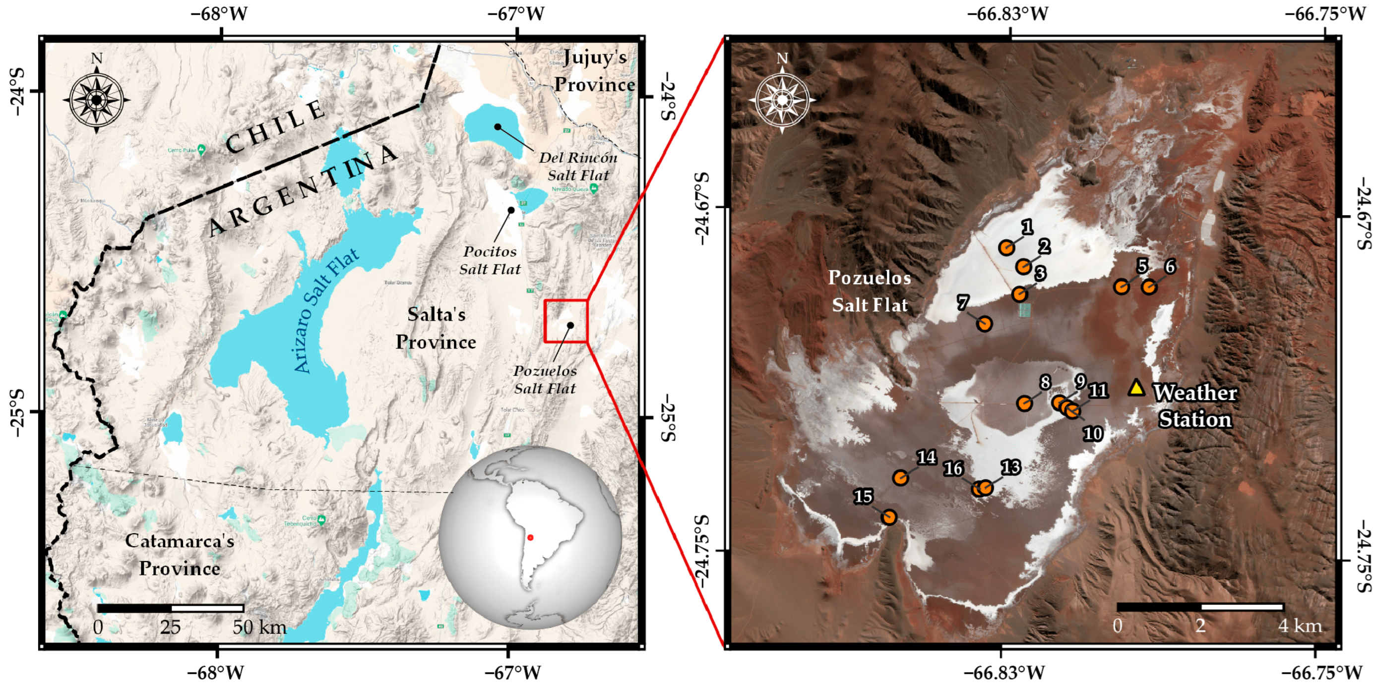
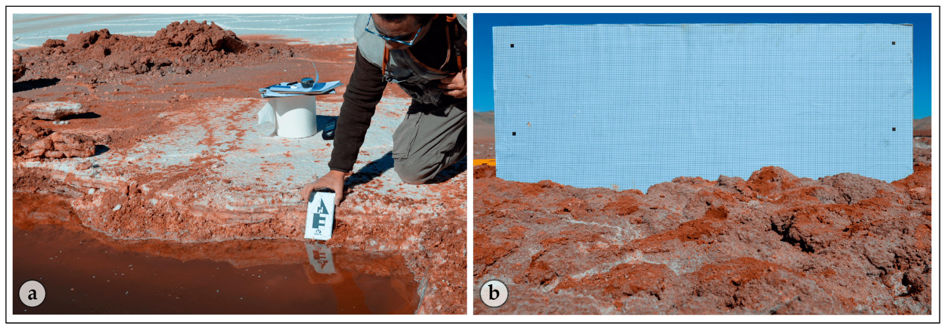
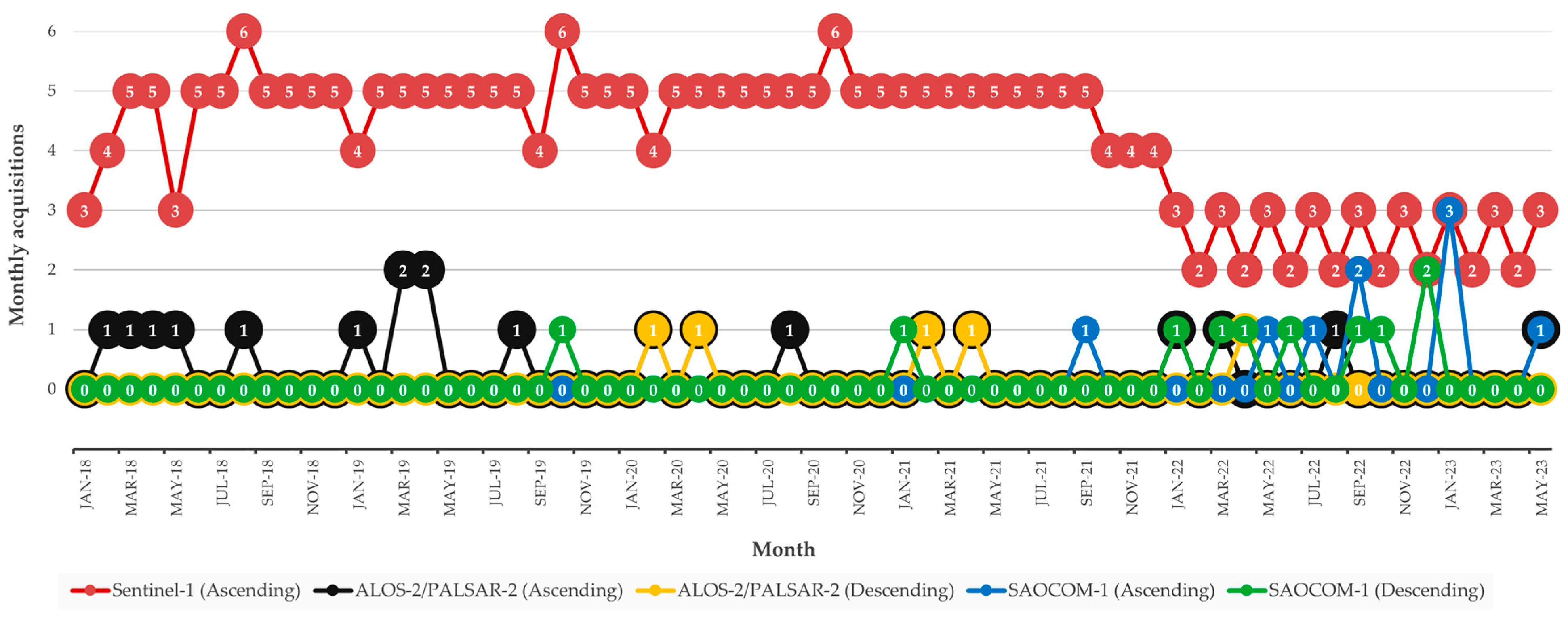
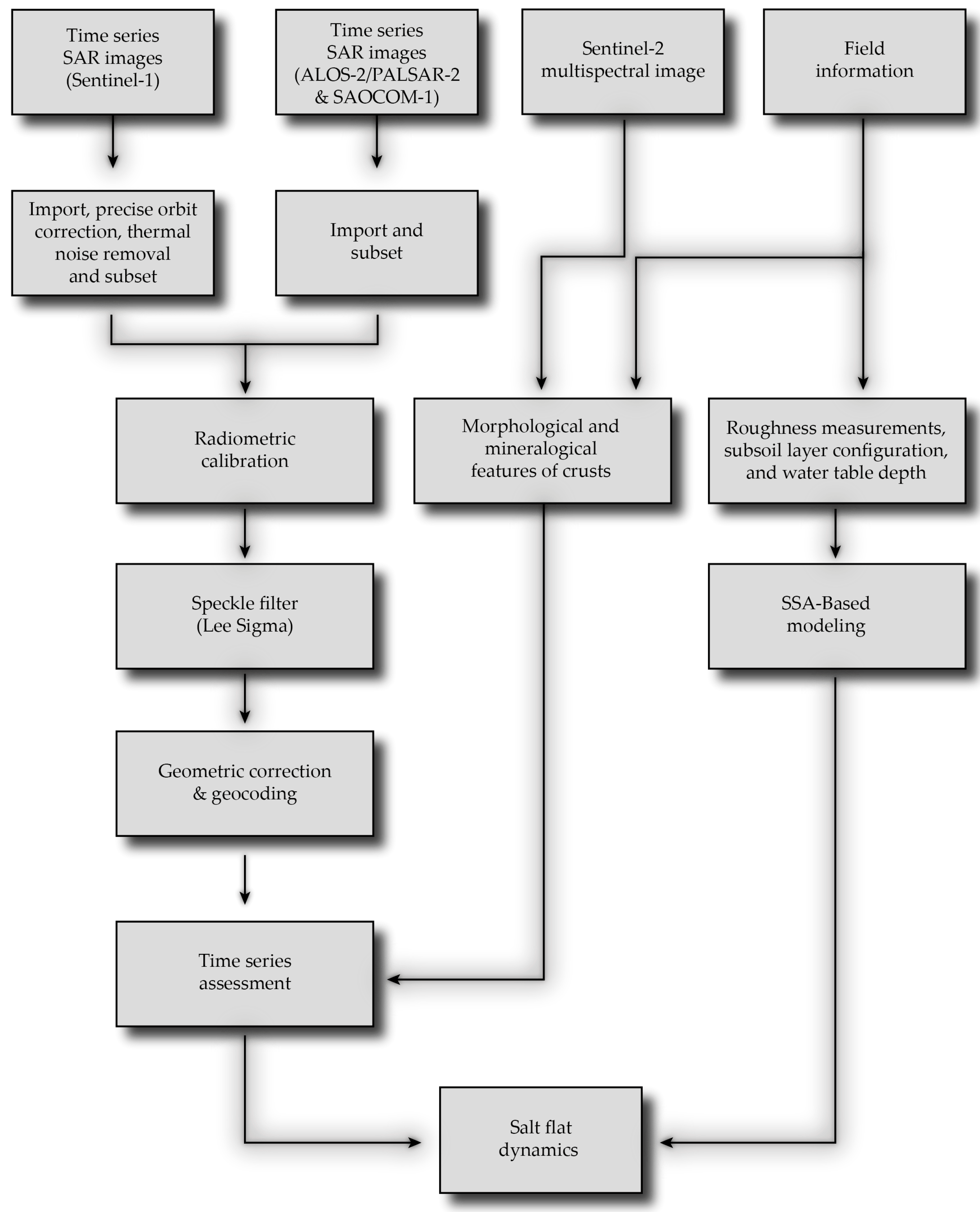
Baseline information for a deeper understanding of crust dynamics is collected through a five-year multi-temporal dataset (January 2018–May 2023) with a dense time series of Sentinel-1 (C-band), ALOS-2/PALSAR-2, and SAOCOM-1 (L-band). Ancillary information from an in situ weather station and from a distributed network of bores aided the interpretation of crust formation and later development. In addition, in situ parameters, such as crust roughness, horizon configuration, water table depth, and brine salinity, were collected at sampling sites across the salt pan by means of a field campaign carried out on 28 and 29 May 2023.

This study is aimed at assessing the capabilities of a scattering model in relating the SAR backscattered signal with the surface and subsurface salt pan configuration of the Pozuelos salt flat located at Puna Salteña in northern Argentina.

The remainder of this paper is organized as follows. The study area and the fieldwork are presented in Section 2.1 and Section 2.2, respectively. Detailed information on SAR image processing, crust classification, backscattering models, and the Bayesian approach for estimating model parameters are presented in Section 2.3 to Section 2.7. The influence of weather on SAR backscattering over time is described in Section 3.1 and Section 3.2. Surface and subsurface modeling are analyzed in Section 3.3 and Section 3.4. Discussion is provided in Section 4, followed by concluding remarks in Section 5.

2. Materials and Methods

2.1. Study Area

The Pozuelos salt flat is located at 3760 m.a.s.l. at Puna Salteña in Salta’s Province (northern Argentina), whose approximate geographical coordinates are 24°40′S and 66°45′W (Figure 1). Its approximate dimensions are 13 km long by 6 km wide in an NE elongated arrangement with an approximate area of 84 km² [33]. Within the salt flat boundaries, a weather station provided daily rainfall from 12 December 2018 to 20 February 2022. Locations of the crust boundaries, sampling sites covering different crust types, and the weather station are shown in Figure 1.

The soil surface is composed of different crusts, each one having different types of roughness and chemical compositions. According to their roughness, crusts are classified as smooth, moderately rough, and very rough, whereas according to their compositions, they are saline or earthy. Saline crusts encompass a halite (NaCl) domain with a smooth surface and the presence of gypsum and borates, in addition to clastic materials. In general terms, there are two domains on the surface of the salt flat: saline crusts and earthy crusts. Saline crusts have a high halite content and low roughness, while earthy crusts are moderate to very rough and contain a mixture of clastic material composed of clay, silt, fine sand, and evaporite minerals to a lesser extent [33].

2.2. Field Sampling and Laboratory Measurements

A total of 16 points of interest (IDs) were initially selected based on the different salt crusts and the feasibility of access. However, sampling site ID-4 was extremely hard to excavate, and site ID-12 was unreachable due to a loose road. Finally, samples were taken at 14 sites (Figure 1).

Trenches at each sampling site were made with an excavator. Trench dimensions are roughly 3.5 m × 1.5 m with 0.15 to 1.0 m depth according to the local water table depth at each sampling location, enabling a good description of the horizon configuration (Figure 2a). The water table depth and the soil temperature were measured at the trenches. This information is important to consider because it sets a limit to the penetration capability of the radar wave due to the high salinity of the brine in the saturated zones. In addition to the measurements mentioned above, samples of the brine were taken for chemical analysis as well as of the soil for bulk and specific densities. Brine salinity was expressed as the weight of Na+ and Cl- ions dissolved in a liter of solution. Even though the brine contained sulfates and other salts in addition to NaCl, NaCl was the principal component with 97% of the total dissolved solids; therefore, the expressions developed for pure NaCl solutions were assumed applicable.

Table 1. Soil features.

Soil Parameter	Measurement
Subsurface temperature (T)	2.1–15 °C
Average salinity (Sb)	(313 ± 2) g/L
Soil bulk density	(0.882 ± 0.003) g/cm3
Soil specific density	(2.05 ± 0.01) g/cm3
Soil porosity	0.569 ± 0.004

resumes the soil features.

Crusts are composed of halite and clastic rocks, whose relative fractions vary according to the crust type and were estimated from samples taken at the top 10 cm for each crust. Halite fraction reached a maximum of 90% for type I crust and decreased to 70%, 55%, and 20% for types II, III, and IV, respectively. For the remaining clastic fraction, sand and clay percentages (S, C) were (30%, 50%), (17%, 50%), (22%, 44%), and (25%, 25%) for types I to IV, respectively.

A number of photographs of a gridded board placed at each sampling location were taken to estimate surface roughness (Figure 2b). Three photographs per site placing the gridded board in two orthogonal transects and a third at the corresponding angle bisector were considered. A supervised edge detector rendered the crust profile, and root mean squared (RMS) height s, correlation length l, and slope s/l were computed [11] as summarized in

Table 2. Average roughness parameters were estimated by placing a gridded board onto the soil and extracting the corresponding contour. Excavator tracks largely disturbed soil crust at site ID-8, so no photographs were taken. A halite polygonal edge was included in the photographs at site ID-10, leading to a non-Gaussian height distribution, so roughness measurements there were disregarded.

Sampling Site ID	RMS Height s [cm]	Correlation Length l [cm]	Slope s/l	Crust Type 1
1	0.137	2.01	0.0685	I
2	0.201	3.31	0.0609	I
13	0.125	3.13	0.0401	I
9	4.32	9.62	0.450	II
5	0.992	4.67	0.219	III
7	1.31	5.88	0.214	III
14	0.916	5.51	0.177	III
15	0.841	4.96	0.173	III
16	1.28	6.59	0.197	III
3	3.51	9.89	0.350	IV
6	5.05	8.11	0.630	IV
11	3.74	9.79	0.399	IV

¹ See Section 2.5 Field Classification of Crusts.

. Skewed or non-Gaussian profiles were disregarded, mostly due to halite polygonal edge inclusions or issues with the leveling of the board at sites with very rough crusts. The sample power spectrum of the profiles was determined as exponential for ID-1, ID-2, and ID-13 (type I) and Gaussian for the remaining sites (types II–IV).

2.3. SAR Images

For this study, 275 Interferometric Wide Swath (IW) mode, Ground Range Detected (GRD) Sentinel-1, 22 Fine mode Dual polarization (FBD) ALOS-2/PALSAR-2 and 19 Stripmap Dual and Quad pol SAOCOM-1 level 1 images were processed. Figure 3 shows the monthly cumulative number of scenes acquired between January 2018 and May 2023. Scene availability from January 2022 was affected by the failure and later end of the Sentinel-1B satellite mission [34].

Instrument noise floor diminishes sensitivity for weak backscatters. As for Sentinel-1, instrument performance for the IW mode has a marked dependence on the incidence angle [35], with a noise floor better than −28.8 dB at VH at the incidence angle of the observations. ALOS-2/PALSAR-2 noise floor is −36 dB at HH and −46 dB at HV, far beyond the lower backscattering coefficients found in the study area [36]. Finally, SAOCOM-1 performance is better than −28 dB and −34 dB for dual polarization and quad polarization modes, respectively [37].

2.4. Methodology

Image processing involved the usual preprocessing steps for all images starting with importing the files, orbit correction and thermal noise removal for Sentinel-1, and spatial subset selection. Then, images were radiometrically calibrated, except for SAOCOM-1, so that images are delivered calibrated. Subsequently, a Lee Sigma filter with a 17 × 17 pixel window was used to improve radiometric quality. Finally, to transform the images from slant range to ground range, geometric terrain correction was applied by means of an SRTM 1Sec HTG digital elevation model and cubic-convolution interpolation, resulting in an image with a nominal pixel size of 10 m × 10 m. Finally, output bands of backscattering coefficients for VV and VH were generated for Sentinel-1, HH, and HV for ALOS-2/PALSAR-2, HH, and HV for dual-pol SAOCOM-1 and the corresponding four combinations for quad-pol SAOCOM-1. Local incidence angle bands were generated accordingly. The methodology flowchart is shown in Figure 4.

The classification of the crusts carried out by [33] in 2020 was refined through a supervised classification of a Sentinel-2 multispectral image on 30 May 2023 to mitigate human intervention, such as roads, excavations, etc., ever since.

Field measurements were used for two purposes. Roughness parameters, soil bulk features, and soil temperature were inputs for the scattering model, whereas brine salinity and water table depth were used to compare against model parameters retrieved by means of Bayesian inference.

2.5. Field Classification of Crusts

Six different crusts (types I to VI) based on surface and chemical features gathered in situ were classified over the Pozuelos salt flat (Figure 5a). Types I and V are smooth halite crusts with a typical polygonal edge pattern. Type II is an earthy, very roughed crust at the depocenter, covered with large, sharp protrusions overlying a halite layer. Type III is an earthy, moderately roughed, brittle crust with rounded bosses and an overlying discontinuous halite layer. Type IV is an earthy, angular-shaped crust with large roughness and a centimeter-scale underlying porous pattern. Finally, type VI is an earthy crust associated with borates [33]. In optical images (visible range), saline crusts (halite) exhibit high reflectance (white areas in true color images), while earthy crusts show moderate reflectance (brown-gray areas in true color images) (Figure 5b). Overall, crust differentiation is conveyed to the microwave response at C-band VV by means of surface roughness. In other words, the larger the roughness, the larger the backscattering coefficient displayed in SAR images. Thus, halite crusts (types I and V) resulted in low backscattered coefficients (dark areas in SAR images) compared to crusts with moderate or large roughness, such as types II to IV (bright areas in SAR images) (Figure 5c). However, some differences arise, in the sense that some crusts’ boundaries classified by the optical image fade off in the radar one. The opposite is also true, mainly at the L-band (not shown), where some radar features might not be identified at optical bands. Figure 5c shows the unfiltered radar image with a clear response of the scatters related to the surface roughness, and Figure 5d displays the result after applying the Lee Sigma filter to the radar image for speckle reduction.

Figure 6 corresponds to on-site photographs of the main salt crusts in the Pozuelos salt flat, where the previously mentioned different roughness can be observed, which are also visible in the SAR images (Figure 5c,d).

On 29 and 30 May 2023, a field campaign was carried out with the objective of collecting data relevant to the radar wave scattered by the salt flat. The campaign was scheduled during this period to coincide with the overpass of ALOS-2/PALSAR-2 satellite on 30 May, SAOCOM-1 on 1 June, and close to the Sentinel-1 acquisition on 25 May.

Table 3. Backscattering coefficients at ID-1, ID-7, and ID-16 averaged over a 50-m radius area for Sentinel-1, ALOS-2/PALSAR-2, and SAOCOM-1 with a 50% confidence level.

Sensor (Mode)	Acquisition Date	Orbit Pass	ID	Incidence Angle	HH [dB]	HV [dB]	VH [dB]	VV [dB]
Sentinel-1 (IW GRD)	05/25/23	Ascending	1	40.4	-	-	−27.9 ± 0.2	−14.85 ± 0.06
			7	43.0	-	-	−20.4 ± 0.3	−9.01 ± 0.09
			16	43.3	-	-	−20.1 ± 0.3	−9.2 ± 0.4
ALOS-2/ PALSAR-2 (FDB)	05/29/23	Ascending	1	33.3	−18.6 ± 0.7	−31.2 ± 0.5	-	-
			7	36.0	−9.4 ± 0.4	−21.5 ± 0.4	-	-
			16	36.2	−9.2 ± 0.9	−19 ± 2	-	-
SAOCOM-1 (Quad pol)	06-01-2023	Descending	1	26.6	−18.8 ± 0.7	−30.6 ± 0.7	−30.6 ± 0.9	−18 ± 1
			7	24.7	−8.7 ± 0.9	−20.5 ± 0.6	−20.9 ± 0.9	−7.5 ± 0.8
			16	24.0	−6 ± 1	−17 ± 2	−17 ± 2	−5 ± 1

summarizes the average backscattering coefficients for sampling sites ID-1, ID-7, and ID-16 from the mentioned radar images. Related uncertainties have been calculated as 25% and 75% percentiles (i.e., 50% confidence level).

2.6. Small Slope Approximation and Subsurface Salt Pan Model

The Small Slope Approximation has been derived for wave scattering on rough surfaces within the framework of perturbation theory, where the perturbative parameter is the surface slope s/l. More precisely, the scattering matrix R for a two-layer lossy media with rough boundaries can be written as the integral of an unknown functional Φ as

$$\begin{gathered} \mathbf{R}\left(\mathit{p},{\mathit{p}}_0\right)=\int d^2\mathbf{r}{d}^2{\mathbf{r}}^{\prime }\exp \left[-i\left(\mathit{p}-{\mathit{p}}_0\right)\cdot \left(\mathit{r}+{\mathit{r}}^{\prime }\right)-i\left(\alpha \left(\mathit{p}\right)+\alpha \left({\mathit{p}}_0\right)\right)\left(h_1\left(\mathit{r}\right)+h_2\left({\mathit{r}}^{\prime }\right)\right)\right] \\ \times \mathsf{\Phi }\left[\mathit{p},{\mathit{p}}_0;\mathbf{r}:{\mathbf{r}}^{\prime };\left[h_1\left(\mathbf{r}\right)\right];\left[h_2\left({\mathbf{r}}^{\prime }\right)\right]\right] \end{gathered}$$

(1)

which, by means of a perturbative development, is expanded as an integral power series via Taylor expansion of Φ on surface heights h₁ (upper rough surface) and h₂ (bottom). In (1), r and r′ are the vector coordinates for upper and bottom media, respectively, p and p₀ (subscript 0 refers to the incident vector) are the coordinates in momentum space (after Fourier transform), and $\alpha \left(\mathit{p}\right)=\sqrt{\epsilon k^2-{\mathit{p}}^2}$, where $k=2\mathsf{\pi }$λ.

Then, transforming Fourier on Φ and using the unitary property of the scattering matrix [38], the unknown coefficients of the Taylor expansion are found solving order by order the boundary condition at each interface and for each polarization. Up to order 3, as used in this paper, the expansion of Φ yielded 16 terms, which are explicitly stated in [38], Equations (92)–(122).

The SSA is a physically based scattering model that includes both surface and volume scattering mechanisms in the computation of the fully polarimetric backscattering coefficients HH, HV, VH, and VV [39]. Since mean values of the scattered fields are computed, the results depend on the surface parameters RMS height (s) and correlation length (l). Therefore, the scattering model proposed presents seven free parameters: X = {ϵ₁, ϵ₂, d, s₁, l₁, s₂, l₂}, which represent, respectively, the dielectric permittivity ϵ₁ and ϵ₂ of the stratified medium, the average layer thickness d, and the statistical properties of each surface. Specifically, the SSA implemented in this paper followed references [30,31] with a Gaussian power spectrum. In the case of the type I crust, this is driven by the fact that with an exponential power spectrum, no intersection of the contours for Sentinel-1 and SAOCOM-1 occur at all (see Section 3.2).

Establishing the validity domain of the SSA approximation is an open issue and subject to current research. Regarding the feasibility range available in [40], slopes corresponding to type I and III crusts fulfilled the constraints.

Regardless of the different crusts, a common description of the underlying pan configuration over the entire salt flat can be made as a two-layer roughed lossy media subject to be modeled by the SSA. An upper moist layer composed of crystalline halite and clastic materials at a known proportion is above a semi-infinite saturated earthy layer, where the water table is the interface between the two layers (Figure 7). With this model at hand, and the mentioned constraints imposed on the roughness by the SSA, a simulation study on type I and III crusts was carried out.

Measurements of complex permittivity at microwave frequencies usually involve fine techniques, only achievable at the laboratory level. To circumvent this issue, a model for high-salinity brines, where model parameters are brine salinity S_b, volumetric moisture mv, and the bulk parameters shown in Table 1, was used to compute complex permittivities ϵ₁ and ϵ₂ [20] along with the dielectric mixing model described in [16,19]. Since only clastic media are covered by [20], wet halite crystal complex permittivity at C- and L-bands are taken from [17], namely, 7 + 11i and 9 + 31i, respectively, to calculate the dielectric properties of the halite fraction of the crusts.

Regardless of the different crusts, a common description of the underlying pan configuration over the entire salt flat can be made as a two-layer roughed lossy media. An upper moist layer of height d and roughness parameters s₁ and l₁ composed of crystalline halite and clastic materials at a known proportion are above a semi-infinite saturated earthy layer, where the water table is the interface between the two layers (Figure 7) with roughness parameters s₂ and l₂. The lossy features of the media are given by the complex dielectric constants ϵ₁ and ϵ₂. With this model at hand, and the constraints imposed on the SSA by the roughness, type I and III crusts were covered.

2.7. Bayesian Inference

Bayesian inference relies on the use of ancillary or contextual information to constrain a given scattering model (SSA) to actual spaceborne observations, taking into account the uncertainties involved in the observations. An expression for the conditional (“posterior”) probability of measuring a certain set of model parameters, such as the brine salinity S_b and the average layer thickness d, given measurements of backscattering coefficients HH and HV under a dual polarization basis can be obtained from Bayes’ theorem:

$$P\left(S_b,d|HH,HV\right)=\frac{P_{HHHV}(HH,HV|S_b,d\left)P_{S_{b}d}\right(S_b,d)}{P_{HHHV}(HH,HV)}$$

(2)

where P_HHHV(HH, HV|S_b,d) is the “likelihood function”, i.e., the probability of measuring a certain set (HH, HV) of backscattering coefficients given measurements of S_b and d, P_Sbd is the corresponding prior joint density function, and P_HHHV(HH, HV) is a global normalizing factor and the probability of a certain (HH, HV) to be measured. Thus, model parameters are inferred from SAR measurements. The likelihood function is a stochastic version of the scattering model and measures the degree of compatibility between a certain SAR measurement and certain model parameters constrained to the given scattering model. The higher the values of the likelihood, the more likely that the SAR measurement comes from that specific combination of model parameters.

Due to the model’s complexity and its implicit numerical nature, explicitly solving for the posterior in (2) is not possible and one must rely on a sampling algorithm to compute it. Monte-Carlo methods are able to generate samples of the posterior and return a joint plot for any two of the model parameters. The overall shape of the posterior will depend on the sensitivity of each parameter to the model, the error distribution for the likelihood, and the shape of the prior distribution used in the inference. The variance of the posterior at any given confidence level can be computed afterward.

The likelihood takes into account the SSA model as well as the residual speckle noise after filtering. When SAR data are on dB scale, radiometric uncertainties are constant and data distribution can be assumed Gaussian [41], so the likelihood is normally distributed with mean (SSA(X) − (HH, HV)) and standard deviation given by the observation uncertainties summarized in Table 3. These uncertainties are below 10% (except for ID-16) and reflect the quality of the speckle filtering technique. In Section 3.3, the precision of the inference in terms of the backscattering coefficient uncertainties will be discussed.

The parameter vector now coupled with the model in [20] is X = {S_b, mv₁, d, s₁, l₁, s₂, l₂}. Within this feature space, S_b, d, s₁, and l₁ were measured at fieldwork, mv₁ roughly estimated from a 50 MHz dielectric probe and s₂, l₂ estimated from a visual inspection of the overall horizon configuration at the water table depth, resulting in s₂ = 2 × s₁ and l₂ = l₁/2.

Inference ran on subsurface model parameters S_b and d assuming they are independent, i.e., P_Sbd= P_Sb P_d. A Gaussian prior distribution for S_b is possible by means of the dataset reported in [2]. In fact, a mean of 266 g/L and a standard deviation of 34 g/L are reported for Pozuelos salt flat therein. A uniform prior distribution for parameter d was chosen, whose bounds are given by ±20% variations of the minimum and maximum table depth from a two-year-long time series of a number of bores distributed over the salt pan. Finally, 5000 samples of the posterior were computed with the Sequential Monte-Carlo Sampler (SMC) [42] of the Python library PyMC3 [43].

3. Results

3.1. Water Dynamics after Heavy Rainfalls

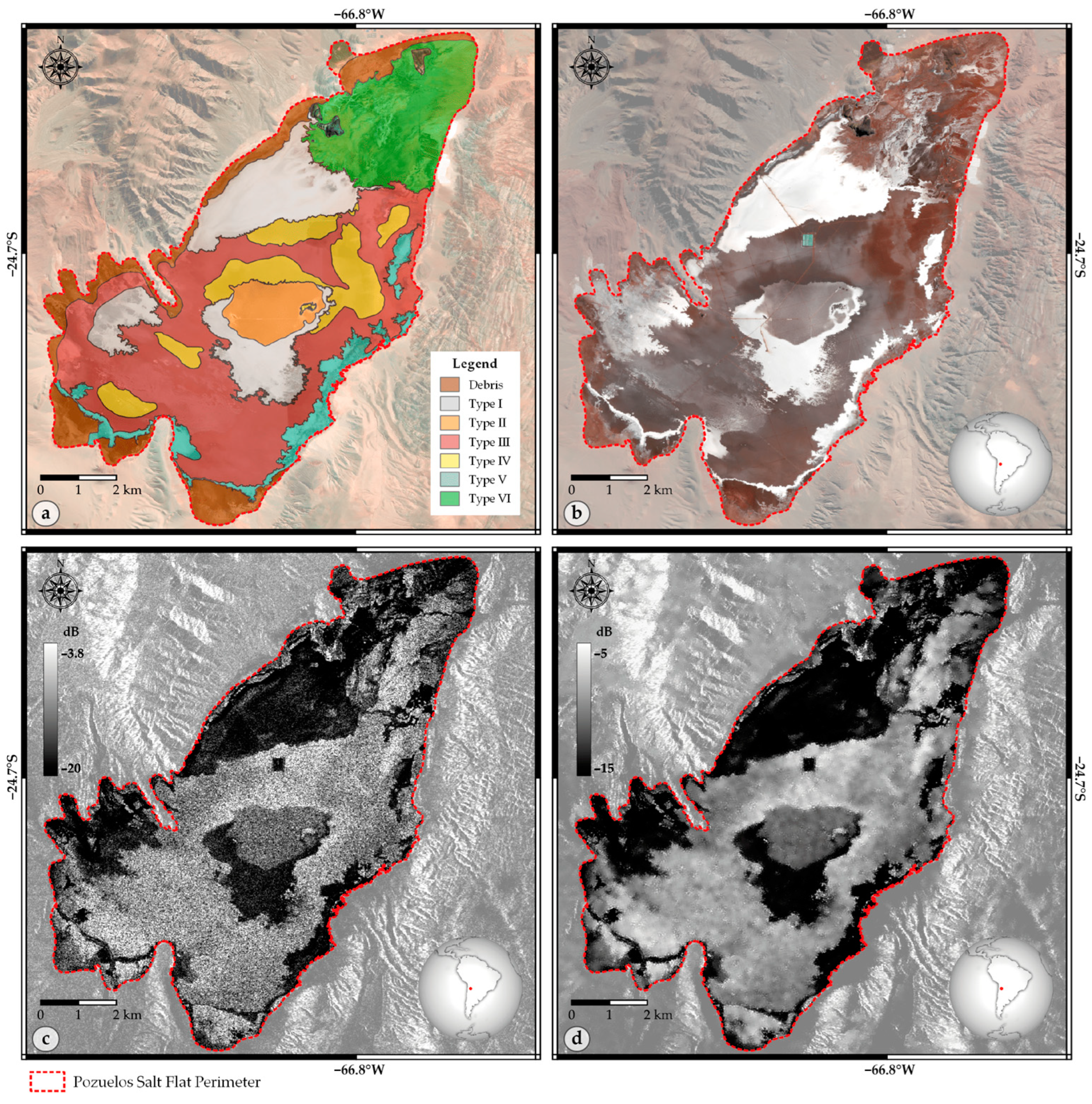
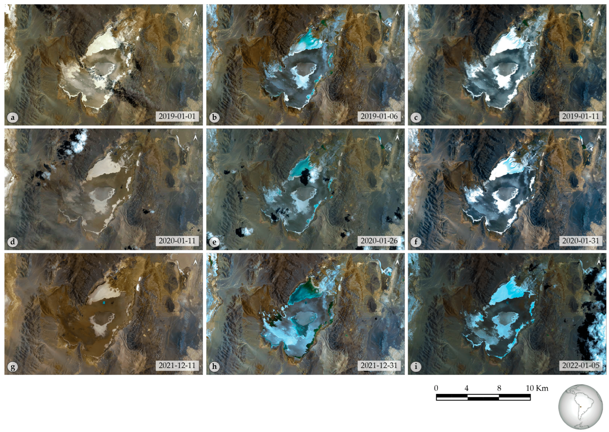
After heavy rainfall events, the salt pan flooded, except for the depocenter, and gradually dried up in the following days. Water remained longer over the earthy crusts than over the halite ones, the latter being covered with a waterbed, and displayed in bluish hues north-, east- and centerward (type I and V crusts) in Figure 8. For those crusts with a large porous pattern, multiple depolarizations increase the backscattering coefficient at cross-polarization when they remain partially filled with water.

3.2. Time Series Analysis

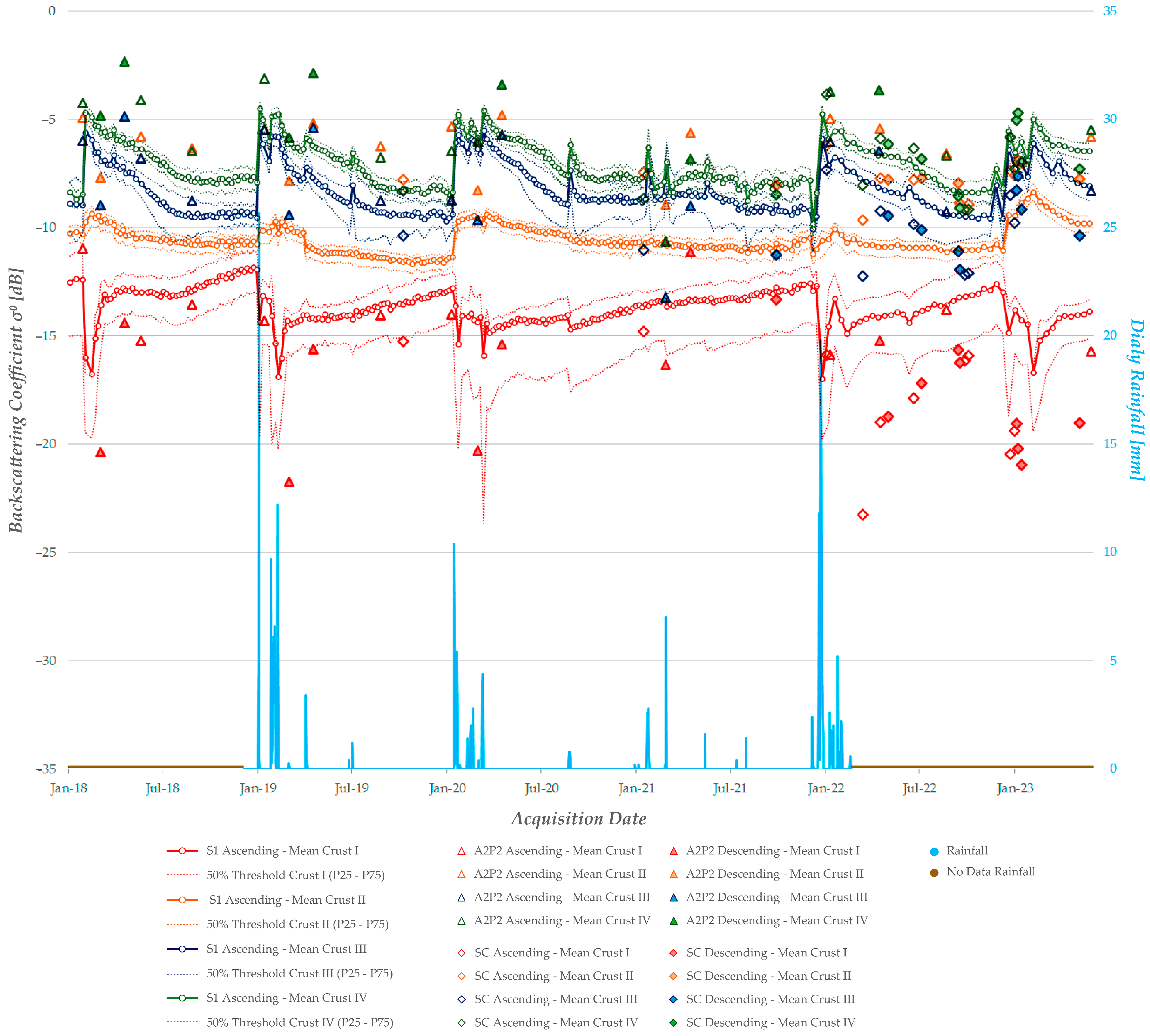
The SAR backscatter dynamics are depicted in Figure 9 and Figure 10, where the average backscattering coefficients for each crust type and the 25th- and 75th-percentile were plotted. Rainfall was also plotted when available. For type II (orange), III (blue), and IV (green) earthy crusts, C-band VV-polarized backscattering coefficient temporal evolution depicted an annual periodic pattern triggered by the summertime rainfalls in January and then an overall decrease until the end of the year. The type I halite crust (red) exhibited the opposite dynamics, with a marked drop at the first heavy rainfall around January and then a steady increase until the end of the year. Among the earthy crusts, type IV had larger backscattering coefficients, followed by those of type III and type II, respectively. The aforementioned trend can be explained with the surface roughness slope summarized in Table 1, where s/l~0.4–0.6 for type IV and s/l~0.2 for type III. Despite the type II crust having a large slope (s/l~0.45), the C-band scatter relies more on the underlying, moderately rough surface than on the protrusions, which are many wavelengths in size at the C-band.

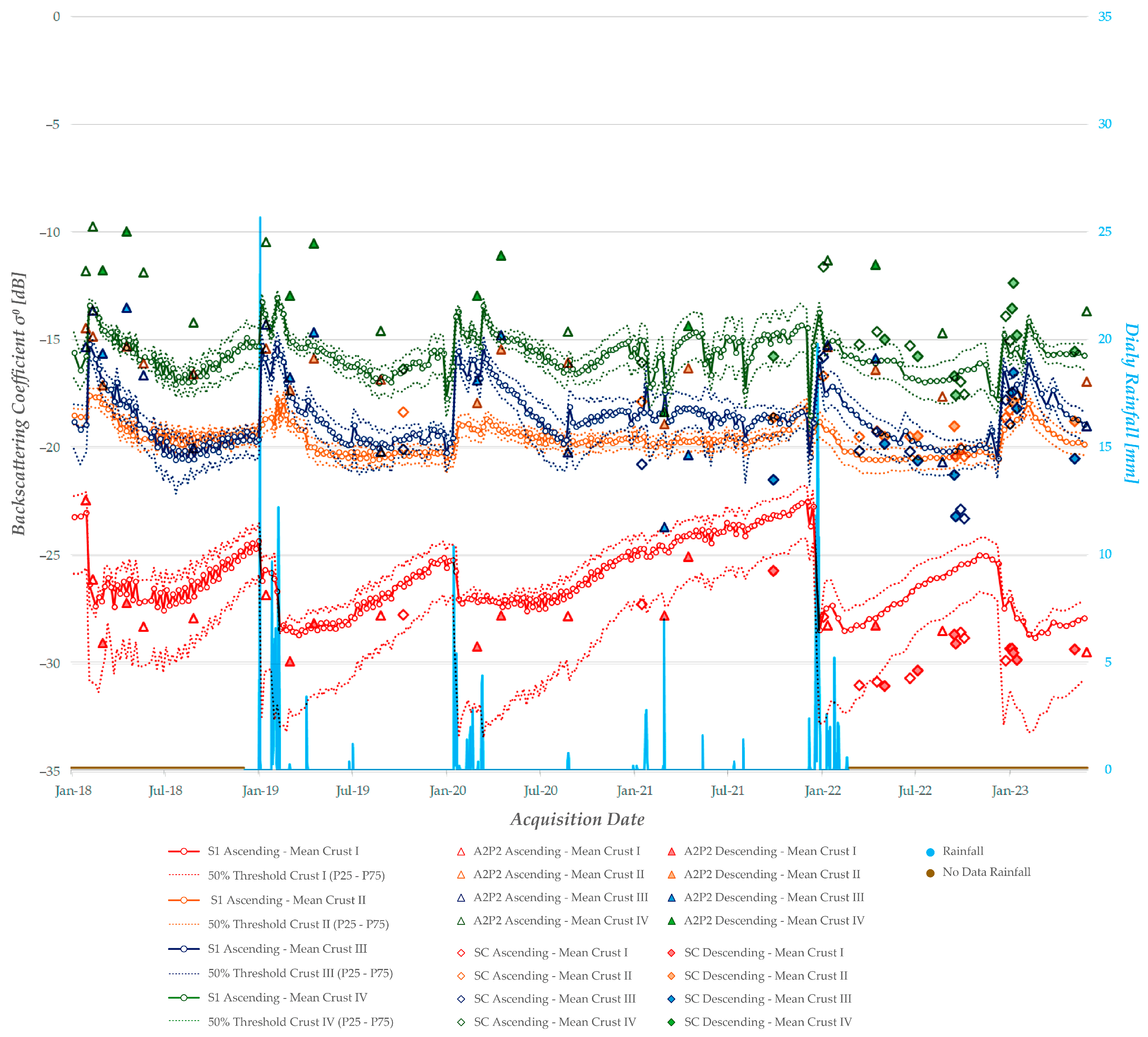
For the cross-polarized case (Figure 10), the annual pattern is similar to the co-polarized one, although type II and III crusts exhibited similar VH-polarized backscattering coefficients, opposite to the co-polarized case where at least a 2 dB difference between those crusts was observed. Also, the larger differences between these crusts occurred close to the rainfall events, when the voids below the bosses in type III crust filled with water, thus enhancing the volume scattering mechanism [11]. In this same respect, the large porous pattern in type IV crust seemed to be responsible for the large backscattering coefficient at VH.

Backscatter dynamics at the L-band are depicted in Figure 9 and Figure 10 with colored triangle and diamond markers. Overall, type I crust is generally lower than the corresponding at the C-band for both the co- and cross-polarized modes. In contrast, type II (orange triangles) and type IV (green triangles) crusts exhibit the opposite, with the co-polarized L-band backscattering coefficients for ALOS-2/PALSAR-2 exceeding those at the C-band as well as most of the SAOCOM-1 ones. For type III, the distinction is less pronounced, at least in the case of ALOS-2/PALSAR-2 data.

In some months, namely August 2019, January 2020, and April 2021, ALOS-2/PALSAR-2 backscattering coefficient for type II (orange triangles) is larger than that of type IV (green triangles). The same is true in some months for SAOCOM-1 (diamond markers). This happened mostly for dried-up crusts and could be related to subsurface scattering mechanisms enhanced by a shallow water table at the depocenter in those months.

At cross-polarization, the backscattering coefficient for types II and IV at the L-band is consistently larger than that at the C-band as in the case of co-polarization. However, the ordering of crust types did not reverse and followed that at the C-band: σ0IV > σ0II > σ0I, and σ0II is usually larger than σ0III. For type III crust, the SAOCOM-1 backscattering coefficients are lower than those observed with Sentinel-1, with one exception on 5 January 2023 where the different orbit pass may explain that VH at the C-band is less than HV at the L-band.

Comparing the temporal curves obtained for the different SAR images, it can be observed that the classification of the crusts is better defined in the co-polarized data (Figure 9) than in the cross-polarization data (Figure 10), where temporal curves intersect for type II and type III crusts, clearly evident in the year 2018.

The backscatter dynamics of the different crusts are driven by the precipitation events, which are very scarce (10 to 50 mm/year in Puna Salteña and 50 to 80 mm/year in Pozuelos Salt Flat) but concentrated in the summertime from December to February [33,44,45], leading to high rates of rainfall that affect salt crusts differently. Type I and V crusts experience a decrease in their backscattering coefficient, reaching a minimum. Water droplets cause a disruption in the crystalline structure of the halite. When exposed to rainfall, the crust smoothens as the crystalline structure dissolves, gradually recrystallizing and increasing its roughness over time.

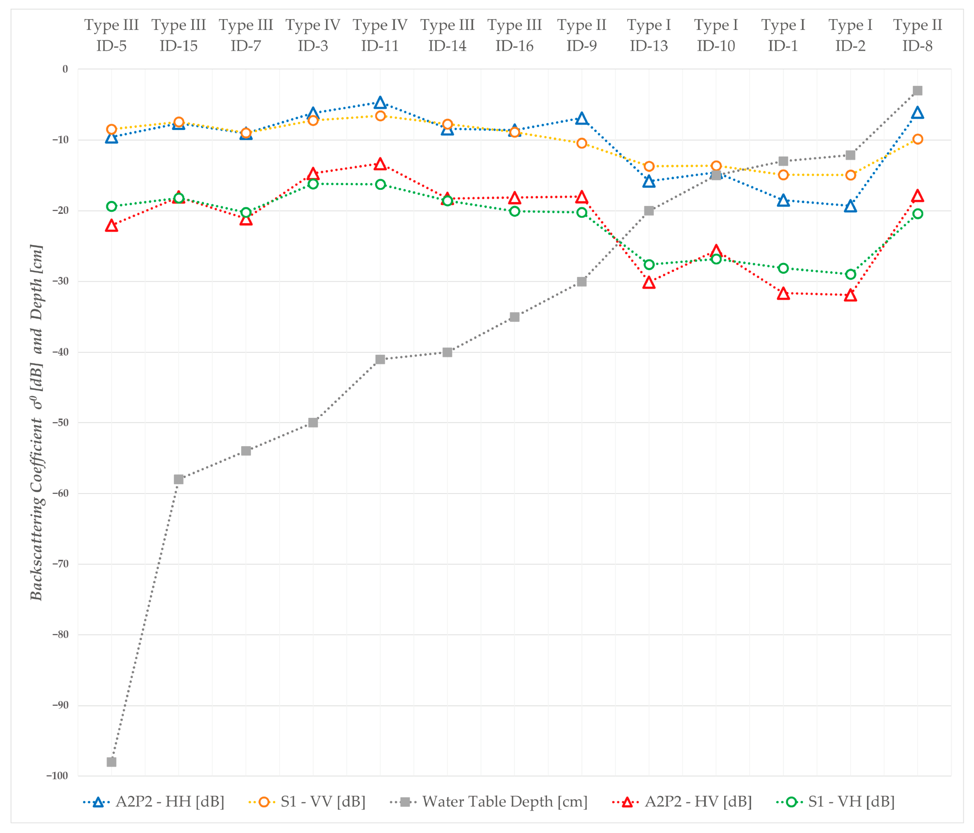
Figure 11 displays backscattering coefficients for Sentinel-1 ascending (VV and VH) and ALOS-2/PALSAR-2 ascending (HH and HV), averaged over a circular area with a 50 m radius at each sampling site, and the corresponding depth of the water table. SAR images and in situ measurements corresponded to the period of the fieldwork. It can be observed that for type I crust, values for the C-band are greater than those of the L-band. However, in earthy crusts (II, III, and IV), values for the C-band are either similar or lower. A subtle correlation of the backscattering coefficient with the depth of the water table is observed, decreasing as the water table becomes shallower. This is consistent with the large attenuation of the propagating waves into a highly lossy media due to the high-salinity brine. When the water table is very shallow, large dielectric contrast onto a very rough upper boundary, as in the case of type II crust, results in a large backscattering coefficient. The dependence of SAOCOM-1 backscattering coefficients on water table depth was very similar to the corresponding ALOS-2/PALSAR-2 shown in Figure 11.

3.3. Upper Layer Roughness from the Two-Layer SSA Model

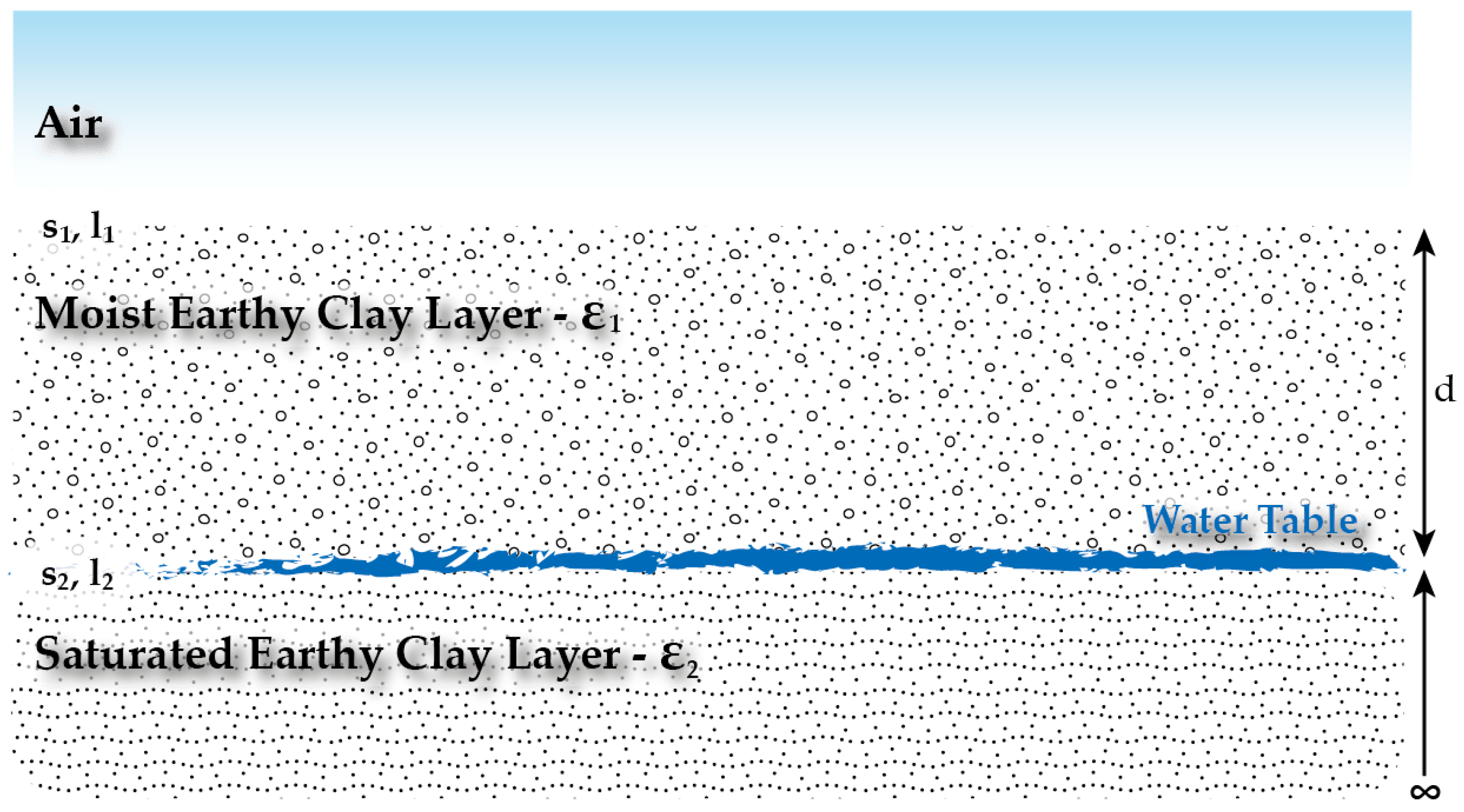
Considering that the C-band has less penetration depth into the soil than the L-band, a first attempt to assess the SSA model in retrieving surface parameters s₁ and l₁ on a type I (ID-1) and two type III (ID-7 and ID-16) crusts was performed. The SSA model was used, considering a layer thickness d given by the water table. With the aid of pictures taken on the soil profile at the trenches, overall observations of the water table inclusions on the soil led to lower layer parameters s₂ = 2 × s₁ and l₂ = l₁/2. A number of model simulations showed that backscattering coefficients have very low sensitivity to s₂ and l₂ variations.

Contour levels in Figure 12 show the model computations (thick contours) for Sentinel-1 (blue) at VV and for SAOCOM-1 (black) at HH. The co-polarized measured backscattering coefficients (dotted contours) are from Table 3. Intersection of measured contours resulted in the (s₁, l₁)-pair combination compatible with the SSA model and the spaceborne observations. With that intersection close to the measured in situ roughness parameters at the red crosses, this first attempt at assessing the SSA model yielded satisfactory outcomes. Similar results were found for the intersection of the cross-polarized backscattering coefficients as well as the combination of Sentinel-1 and ALOS-2/PALSAR-2. Although type I crust is better described by an exponential power spectrum, only a Gaussian one led to intersecting contours as shown in Figure 12a.

3.4. Subsurface Parameter Estimation

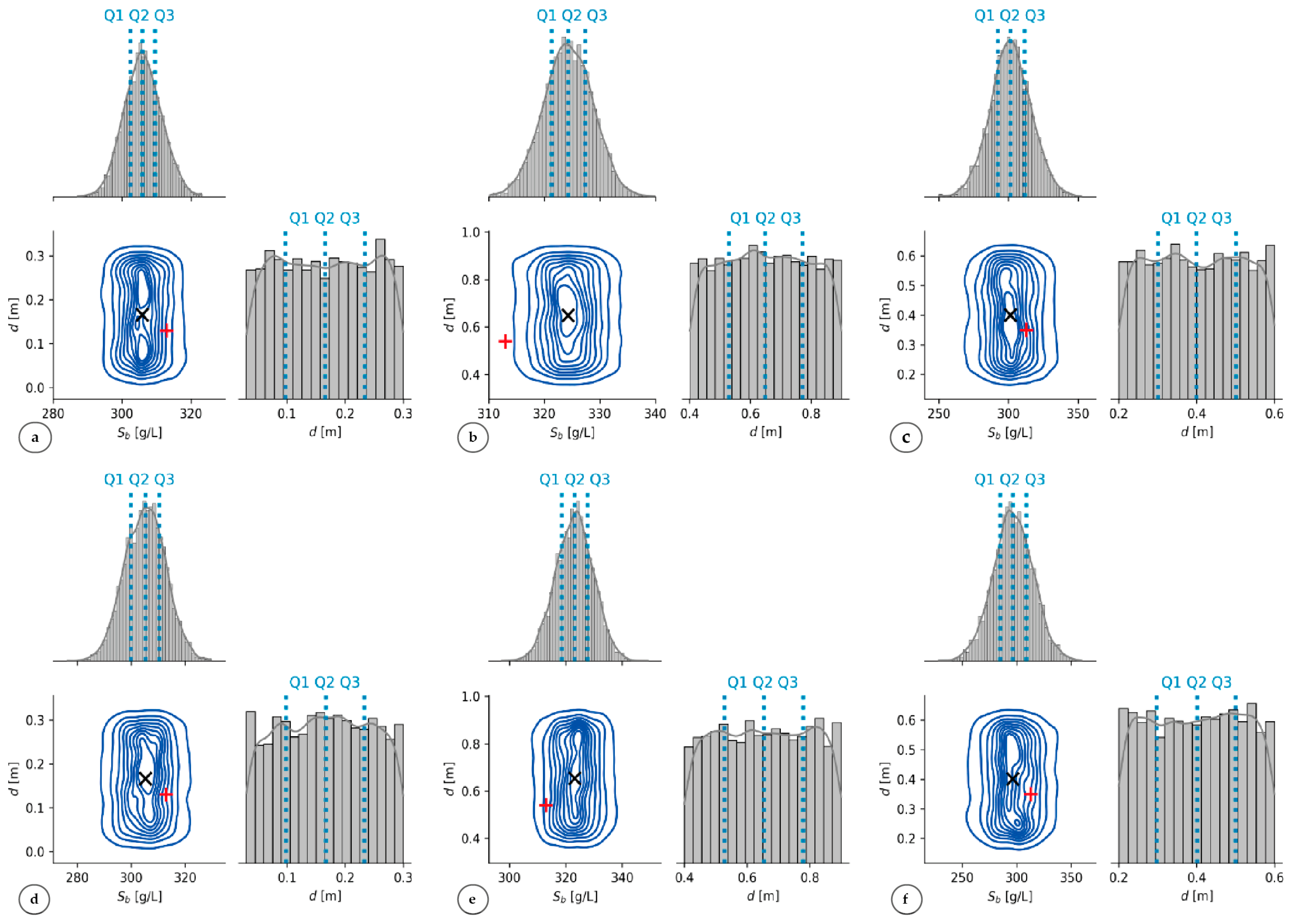
With the SSA enabling the modeling of the backscatter radar response at dual-polarization (HH and HV) and a Bayesian inference scheme at hand, marginal and posterior distributions of the subsurface parameters S_b and d constrained to the radar observations can be computed to assess their compatibility with the measured ones at fieldwork. Figure 13 shows the joint probability generated by sampling out of the posterior as blue contours, whereas the marginal distributions for S_b and d are in the diagonal, with their corresponding Kernel Density Estimation (KDE) indicated in light gray. The quartiles Q1 to Q3, each representing a fourth of the distributed sampled population, are shown as vertical dotted lines. The red plus marks indicate the in situ measurements. Sampling locations are ID-1, ID-7, and ID-16, where the upper panel corresponds to ALOS-2/PALSAR-2 and the lower panel to SAOCOM-1. The lowest contour drawn is 0.05, such that the integral over the area within is 0.95.

The extent of the posterior is overall related to the variance of the likelihood given by the uncertainties of the measured HH and HV. Thus, the more precise the measured backscattering coefficient, the less extended the posterior and, therefore, the more precise the parameter estimation. Two contrasting cases are given by ID-1 and ID-16, both for SAOCOM-1. While the posterior computed at ID-1 spanned a small area, the one corresponding to ID-16 spanned an area roughly four times bigger, in accordance with the HH and HV relative errors for these sites, as readily computed from Table 3. The variance of the priors for S_b and d are given in [2] and by a two-year-long record of water table depths, respectively, as stated in Section 2.7.

Overall, the measured parameters are close to the median (Q2 quartile, black cross marker). Additionally, in those posteriors that are multimodal, they correspond to one of the maximums of probability. The sharp decrease of the KDE for the parameter d is in accordance with the bounds of the uniform distribution used prior.

The estimation of the salt concentration of brine is very precise since the modes of the probability are vertically aligned with almost no spread. Accuracy computed as (S_{b_Q2} − S_{b_insitu})/S_{b_insitu} ranges from 2% to 5%, with that of ID-16 (SAOCOM-1) being the poorer agreement. When replacing Q2 with the mode, accuracy slightly improves, ranging from 2% to 4%. Similar results have been found for the remaining sampling sites, with accuracies ranging from 1% to 8% for both Q2 and mode estimators. On the other hand, the estimation of water table depth has one or two elongated areas corresponding to the larger contour levels of the posterior distribution, each one compatible to some extent with the measured backscattering coefficients.

4. Discussion

The multi-temporal analysis of backscatter variations in SAR imagery over the Pozuelos salt flat reveals a strong relationship with precipitation data recorded at the on-site weather station (Figure 9 and Figure 10). A plausible explanation for this observation is the alteration of salt crust properties due to the interaction between their constituent minerals and liquid water droplets. The physicochemical characteristics of the diverse salt crusts are likely influenced by the presence of water, leading to changes in their backscattering behavior.

The backscatter dynamics of the different crusts were driven by the precipitation events, which are very scarce (10 to 50 mm/year in Puna Salteña and 50 to 80 mm/year in Pozuelos salt flat) but concentrated in the summertime from December to February [32,43,44], leading to high rates of rainfall that affect salt crusts differently. Type I and V crusts, mostly composed of halite, underwent a dissolution process due to rainfall, resulting in a smoother surface, which implied a sharp decrease in the backscattering coefficient. Remarkably, observed rates of decrease are very similar across the different summertime periods in 2019–2022, ranging from 0.6 dB to 0.9 dB per 10 mm of daily rainfall. Subsequent drying led to the growth of salt crystals, which, in turn, increased the surface roughness and consequently raised the backscatter response [25,46].

In addition to the growth of salt crystals, the formation and later development of halite polygons led to an increase in the centimeter-scale roughness over time. This contribution to the overall surface roughness, as seen by the SAR, was not accounted for in the crust profiles with the gridded board, therefore explaining the mismatch found in the intersection of the SSA-based contour levels and the fieldwork estimate.

Conversely, earthy crusts (types II to IV) exhibited an increase in their microwave response, reaching a maximum on the first rainy days after a long dry period (Figure 9 and Figure 10). The rates of increase of the type III and IV crusts are about 0.3 dB to 1.2 dB per 10 mm of daily rainfall. A saturation value slightly above −5 dB at the C-band VV is consistently reached by the type IV crust. Although naturally rougher than halite crust, these crusts exhibited a greater resistance to rain due to their hardness. However, they also contained halite crystals in their composition, and some were covered with a halite layer, which dissolved upon contact with rainfall, resulting in a layer with increased roughness due to the formation of pores. Over time, these pores became refilled through the halite crystallization process [47,48]. In addition, large pores remain filled with water, increasing the dielectric constant of the surface prior to water evaporation or vertical runoff. The size and extent of the pores are also related to the amount of backscattering power at cross-polarization.

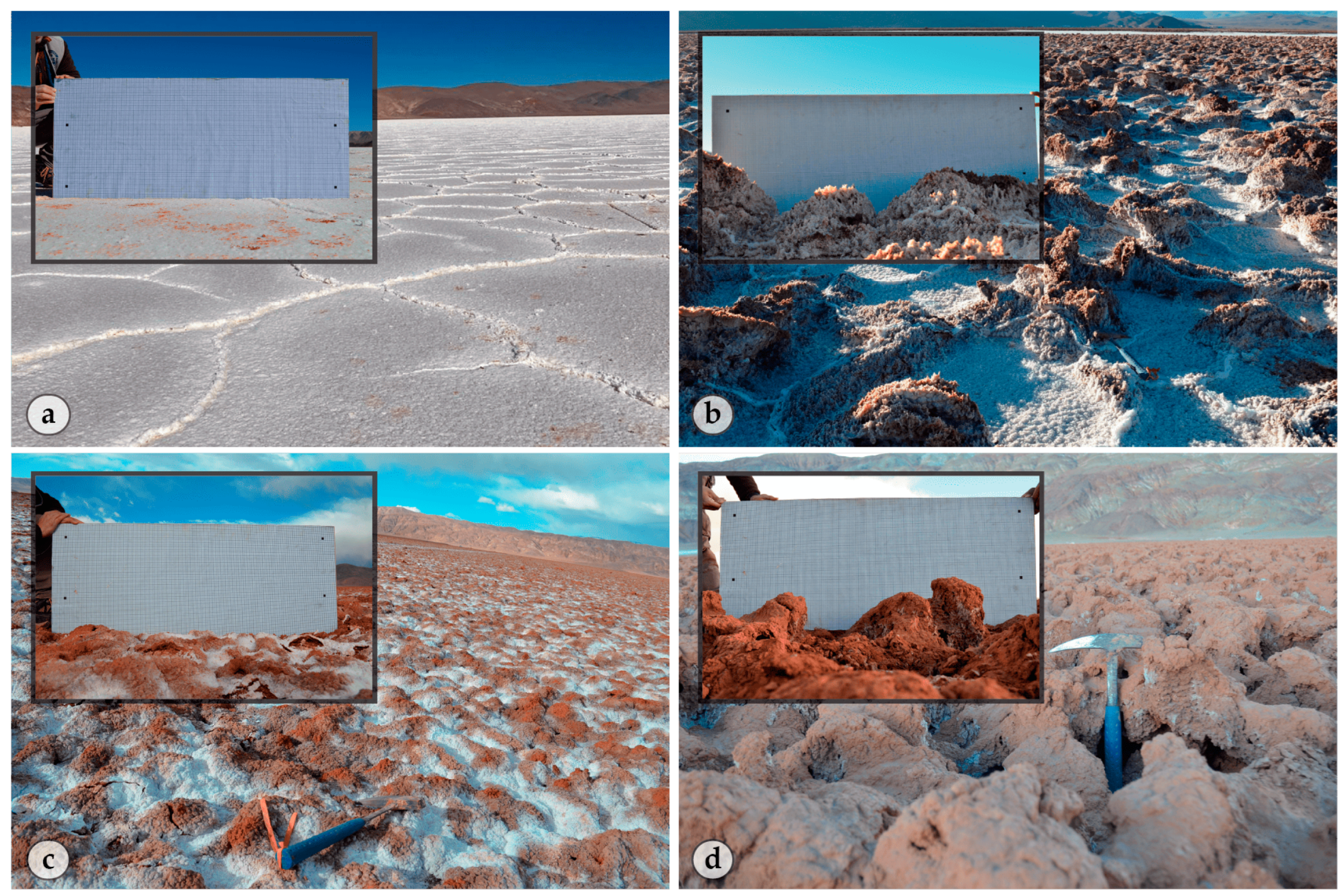
The effects of rainfall on salt crusts are discussed in [48], where it is indicated that thick salt crusts with significant surface relief (>10 cm) are primarily formed by rainfall, which is consistent with the increase in the backscatter coefficient due to a marked increase in surface roughness observed in crust types II, III, and IV. A process known as efflorescence, by which mineral salts crystallize on the surface of a material when the water containing them evaporates, modifies the surface roughness afterward. This occurs naturally when brine penetrates and then evaporates, leaving the salts deposited on the surface, thus covering the underlying relief. Therefore, the surface smoothens and decreases its backscatter. Efflorescence can appear as a white or crystalline layer on the surface (e.g., Figure 6c).

Regarding the backscatter response at the L-band, type II crust backscattering coefficients were above type III, indicating that wavelength–size protrusions at the depocenter largely contributed to the backscatter. The lack of pores in type II prevented this behavior from being observed at HV polarization.

Remarkably, co-polarized backscattered power at the L-band was larger than that of the C-band for the type II and IV earthy crusts, indicating some overall large-scale roughness superimposed to a small-scale Gaussian power spectrum, despite the different incidence angles (34° for ALOS-2/PALSAR-2 and 41° for Sentinel-1). Type III did not display a clear trend, since it varied below and above the corresponding dynamics at the C-band. This seemed to be indicative of multiscale roughness. On the other hand, surface roughness on halite crusts seemed to be of single scale, since L-band backscattering coefficients were systematically lower with respect to that of the C-band (the normalized roughness k × s at the L-band is lower than at the C-band for the same roughness s, i.e., for single scale surfaces). The wavenumber k is defined as 2π/λ. Exponential and Gaussian power spectrums related to type I and type II to IV crusts, respectively, were indicative of the different physicochemical processes related to both the halite and earthy crust growing.

Crust classification with a dense time series at the C-band was better suited with the co-polarized backscatter response (Figure 8) than that of the cross-polarized one (Figure 9), where differentiation between type II and type III crusts may be misleading. A potential radar characterization of crusts was first introduced by [26] as the monthly rate of increase of co-polarized backscattering coefficient at the C-band over large no-rainfall periods. For the type I crust analyzed in this work, the mentioned rate is around 0.2 dB/month, very different from the rates of 1–2 dB/month found in [26] corresponding to a soft pan crust with thrust polygons, possibly indicating different local features such as brine concentration, water availability, and/or solar radiation patterns. An additional overall feature of crust dynamics might be the rate of variation around the summertime heavy rainfalls observed in the backscattering coefficient at the C-band, which seemed very uniform across the seasons for the halite crust. More research is needed in this regard for the earthy crusts.

Enhanced contrast of the backscattering coefficients among the different crust types is observed by comparing images acquired around heavy rainfall events, which are concentrated in austral summertime. Thus, the optimal period for radar characterization of highland salt flats is in late December and early March, on a yearly basis.

Inference of the subsurface model parameters brine salinity and average layer thickness were conducted on the posterior. The overall extent of the posterior and, therefore, the precision of the model parameters that are estimated with, depends primarily on the variance of the likelihood, which is ultimately related to the speckle filtering technique and the spatial homogeneity of the backscatter. In effect, backscatter heterogeneity hinders the efficiency of the speckle filter by adding variance other than the expected from the coherent illumination of the SAR. Thus, the heterogeneity of the backscatter itself is statistically different from the one that speckle filters were designed to deal with. To circumvent this shortcoming, sampling sites over suitable homogeneous areas of the crust surfaces were taken into consideration. The final uncertainties in the backscattering coefficients were similar to the 0.5 dB precision (stability) of the radar sensors ALOS-2/PALSAR-2 [49] and SAOCOM-1 [50].

While the salt concentration of subsurface brine was estimated precisely and with an accuracy better than 8% when the median (Q2) was considered, a multimodal or elongated posterior anticipated water table depth estimation to be more of a struggle. Besides dielectric loss driven by the salt concentration of the brine, clay material in the soil composition also reduces the penetration capabilities of SAR backscatter at the L-band [47]. Therefore, when considering the water table, a weak correlation between the backscattering coefficients and the water table depths was expected (Figure 11). Polarimetric observables, such as the co-polarized phase difference used to gain insight into the feasibility of water table depth estimation [27], required full-polarimetric SAR images, which are largely less available than dual polarimetric images, such as those used in this paper for subsurface parameter retrieval.

In two-layered media, resonances of the radar wave occur as it repeatedly bounce between the media boundaries, with a strong dependency on the layered geometry under study [51]. However, simulation studies on low-loss media showed that attenuation played a key role in fading the power returned for layer distances beyond half wavelength [39]. Yet, the high loss of the salt pan prevented this resonance effect from happening even in the case of type I crust with the shallowest water table. Furthermore, this was also related to the lack of sensitivity of the backscattering power in changing the lower layer roughness found in the simulation study carried out in this paper.

5. Conclusions

Supported by a dedicated field campaign and the processing of 316 SAR images, the dynamics of a highland salt flat have been characterized as a yearly cycle closely linked to summertime rainfalls, which alter roughness configuration depending on the growth process and chemical composition of the crusts.

C-band co-polarized (VV) long-term backscatter response has proven to be effective in differentiating crusts, although a quantitative classification in this respect requires more research. On the other hand, cross-polarization (VH) seems a good proxy for pore patterns when radar imagery close to rainfall events is available.

This paper also demonstrated the potential for subsurface estimation with L-band dual-polarization images, constrained to crusts compatible with the feasibility range of the layered model at hand. Compared with available studies on salt flats with spaceborne radars, this research provided a new perspective on using microwave scattering modeling on dual polarimetric SAR data over salt flats and allowed for better exploitation of radar imagery from existing and upcoming satellite radar missions.

Coupling available multi-sensor SAR data with scattering models allows for the mapping of surface and subsurface configuration of a highland salt pan in a cost-efficient way. This integration could be beneficial for lithium exploration in these environments.

References

1. Clavijo, A.; Díaz Paz, W.F.; Lorca, M.; Olivera Andrade, M.; Iribarnegaray, M.A.; Garcés, I. Environmental Information Access and Management in the Lithium Triangle: Is It Transparent Information? J. Energy Nat. Resour. Law 2022, 40, 293–314. [Google Scholar] [CrossRef]
2. Steinmetz, R.L.L.; Salvi, S. Brine Grades in Andean Salars: When Basin Size Matters a Review of the Lithium Triangle. Earth Sci. Rev. 2021, 217, 103615. [Google Scholar] [CrossRef]
3. Lorca, M.; Andrade, M.O.; Escosteguy, M.; Köppel, J.; Scoville-Simonds, M.; Hufty, M. Mining Indigenous Territories: Consensus, Tensions and Ambivalences in the Salar de Atacama. Extr. Ind. Soc. 2022, 9, 101047. [Google Scholar] [CrossRef]
4. Weinberg, M. The Off-Sites of Lithium Production in the Atacama Desert. Extr. Ind. Soc. 2023, 15, 101309. [Google Scholar] [CrossRef]
5. Fornillo, B.; Lampis, A. From the Lithium Triangle to the Latin American Quarry: The Shifting Geographies of de-Fossilisation. Extr. Ind. Soc. 2023, 15, 101326. [Google Scholar] [CrossRef]
6. Moreno-Brieva, F.; Marín, R. Technology Generation and International Collaboration in the Global Value Chain of Lithium Batteries. Resour. Conserv. Recycl. 2019, 146, 232–243. [Google Scholar] [CrossRef]
7. Lindagato, P.; Li, Y.; Macháček, J.; Yang, G.; Mungwarakarama, I.; Ndahimana, A.; Ntwali, H.P.K. Lithium Metal: The Key to Green Transportation. Appl. Sci. 2022, 13, 405. [Google Scholar] [CrossRef]
8. Cabello, J. Reserves, Resources and Lithium Exploration in the Salt Flats of Northern Chile. Andean Geol. 2022, 49, 297–306. [Google Scholar] [CrossRef]
9. Sabins, F.F., Jr.; Ellis, J.M. Remote Sensing: Principles, Interpretation, and Applications; Waveland Press: Long Grove, IL, USA, 2020; ISBN 1478645067. [Google Scholar]
10. Lillesand, T.; Kiefer, R.W.; Chipman, J. Remote Sensing and Image Interpretation; John Wiley & Sons: Hoboken, NJ, USA, 2015; ISBN 111834328X. [Google Scholar]
11. Ulaby, F.T.; Long, D.G.; Blackwell, W.J.; Elachi, C.; Fung, A.K.; Ruf, C.; Sarabandi, K.; Zebker, H.A.; Van Zyl, J. Microwave Radar and Radiometric Remote Sensing; University of Michigan Press: Ann Arbor, MI, USA, 2014. [Google Scholar]
12. Flores-Anderson, A.I.; Herndon, K.E.; Thapa, R.B.; Cherrington, E. SAR Handbook: Comprehensive Methodologies for Forest Monitoring and Biomass Estimation; NASA: Washington, DC, USA, 2019. [Google Scholar]
13. Franceschetti, G.; Lanari, R. Synthetic Aperture Radar Processing; CRC Press: Boca Raton, FL, USA, 2018; ISBN 0203737482. [Google Scholar]
14. Lu, J.; Mittra, R. Design Technology of Synthetic Aperture Radar [Book Review]. IEEE Antennas Propag. Mag. 2020, 62, 124–125. [Google Scholar] [CrossRef]
15. Woodhouse, I.H. Introduction to Microwave Remote Sensing; CRC Press: Boca Raton, FL, USA, 2017; ISBN 1315272571. [Google Scholar]
16. Lasne, Y.; Paillou, P.; Freeman, A.; Farr, T.; McDonald, K.C.; Ruffie, G.; Malezieux, J.-M.; Chapman, B.; Demontoux, F. Effect of Salinity on the Dielectric Properties of Geological Materials: Implication for Soil Moisture Detection by Means of Radar Remote Sensing. IEEE Trans. Geosci. Remote Sens. 2008, 46, 1674–1688. [Google Scholar] [CrossRef]
17. Lasne, Y.; Paillou, P.; Freeman, A.; Farr, T.; McDonald, K.; Ruffie, G.; Malezieux, J.-M.; Chapman, B. Study of Hypersaline Deposits and Analysis of Their Signature in Airborne and Spaceborne SAR Data: Example of Death Valley, California. IEEE Trans. Geosci. Remote Sens. 2009, 47, 2581–2598. [Google Scholar] [CrossRef]
18. Wu, Y.; Wang, W.; Zhao, S.; Liu, S. Dielectric Properties of Saline Soils and an Improved Dielectric Model in C-Band. IEEE Trans. Geosci. Remote Sens. 2014, 53, 440–452. [Google Scholar]
19. Dobson, M.C.; Ulaby, F.T.; Hallikainen, M.T.; El-Rayes, M.A. Microwave Dielectric Behavior of Wet Soil-Part II: Dielectric Mixing Models. IEEE Trans. Geosci. Remote Sens. 1985, GE-23, 35–46. [Google Scholar] [CrossRef]
20. Peyman, A.; Gabriel, C.; Grant, E.H. Complex Permittivity of Sodium Chloride Solutions at Microwave Frequencies. Bioelectromagn. J. Bioelectromagn. Soc. Soc. Phys. Regul. Biol. Med. Eur. Bioelectromagn. Assoc. 2007, 28, 264–274. [Google Scholar] [CrossRef] [PubMed]
21. Ulaby, F.T.; Dellwig, L.F.; Schmugge, T. Satellite Microwave Observations of the Utah Great Salt Lake Desert. Radio Sci. 1975, 10, 947–963. [Google Scholar] [CrossRef]
22. Liu, C.-A.; Gong, H.; Shao, Y.; Yang, Z.; Liu, L.; Geng, Y. Recognition of Salt Crust Types by Means of PolSAR to Reflect the Fluctuation Processes of an Ancient Lake in Lop Nur. Remote Sens. Environ. 2016, 175, 148–157. [Google Scholar] [CrossRef]
23. Aly, Z.; Bonn, F.J.; Magagi, R. Analysis of the Backscattering Coefficient of Salt-Affected Soils Using Modeling and RADARSAT-1 SAR Data. IEEE Trans. Geosci. Remote Sens. 2007, 45, 332–341. [Google Scholar] [CrossRef]
24. Paillou, P.; Sufyar, S.; Freeman, A. The Chott El Djerid, Tunisia: Observation and Discussion of a SAR Phase Signature over Evaporitic Soils. IEEE Trans. Geosci. Remote Sens. 2013, 52, 5798–5806. [Google Scholar] [CrossRef]
25. Frison, P.-L.; Paillou, P.; Sayah, N.; Pottier, E.; Rudant, J.-P. Spatio-Temporal Monitoring of Evaporitic Processes Using Multiresolution C-Band Radar Remote Sensing Data: Example of the Chott El Djerid, Tunisia. Can. J. Remote Sens. 2013, 39, 127–137. [Google Scholar] [CrossRef]
26. Delsouc, A.; Barber, M.; Gallaud, A.; Grings, F.; Vidal-Páez, P.; Pérez-Martínez, W.; Briceño-De-Urbaneja, I. Seasonality Analysis of Sentinel-1 and ALOS-2/PALSAR-2 Backscattered Power over Salar de Aguas Calientes Sur, Chile. Remote Sens. 2020, 12, 941. [Google Scholar] [CrossRef]
27. Liu, C.-A.; Gong, H.; Shao, Y.; Li, B. Detecting the Depth of a Subsurface Brine Layer in Lop Nur Lake Basin Using Polarimetric L-Band SAR. J. Sens. 2015, 2015, 245790. [Google Scholar] [CrossRef]
28. Lasne, Y.; Paillou, P.; August-Bernex, T.; Ruffié, G.; Grandjean, G. A Phase Signature for Detecting Wet Subsurface Structures Using Polarimetric L-Band SAR. IEEE Trans. Geosci. Remote Sens. 2004, 42, 1683–1694. [Google Scholar] [CrossRef]
29. Voronovich, A. Small-Slope Approximation for Electromagnetic Wave Scattering at a Rough Interface of Two Dielectric Half-Spaces. Waves Random Media 1994, 4, 337. [Google Scholar] [CrossRef]
30. Tabatabaeenejad, A.; Moghaddam, M. Bistatic Scattering from Three-Dimensional Layered Rough Surfaces. IEEE Trans. Geosci. Remote Sens. 2006, 44, 2102–2114. [Google Scholar] [CrossRef]
31. Soubret, A.; Berginc, G.; Bourrely, C. Application of Reduced Rayleigh Equations to Electromagnetic Wave Scattering by Two-Dimensional Randomly Rough Surfaces. Phys. Rev. B 2001, 63, 245411. [Google Scholar] [CrossRef]
32. Soubret, A.; Berginc, G.; Bourrely, C. Backscattering Enhancement of an Electromagnetic Wave Scattered by Two-Dimensional Rough Layers. JOSA A 2001, 18, 2778–2788. [Google Scholar] [CrossRef]
33. Martínez, V.R.; Galli, C.I.; Alonso, R.N. Morfología de Las Costras Evaporíticas Del Salar de Pozuelos, Puna Salteña. Rev. Asoc. Geol. Argent. 2020, 77, 163–173. [Google Scholar]
34. European Space Agency End of Mission of the Copernicus Sentinel-1B Satellite. Available online: https://www.esa.int/Applications/Observing_the_Earth/Copernicus/Sentinel-1/Mission_ends_for_Copernicus_Sentinel-1B_satellite (accessed on 3 March 2024).
35. Torres, R.; Navas-Traver, I.; Bibby, D.; Lokas, S.; Snoeij, P.; Rommen, B.; Osborne, S.; Ceba-Vega, F.; Potin, P.; Geudtner, D. Sentinel-1 SAR System and Mission. In Proceedings of the 2017 IEEE Radar Conference (RadarConf), Seattle, WA, USA, 8–12 May 2017; IEEE: Piscataway, NJ, USA, 2017; pp. 1582–1585. [Google Scholar]
36. JAXA/EORC Calibration Result of ALOS-2. Available online: https://www.eorc.jaxa.jp/ALOS-2/en/calval/calval_index.htm (accessed on 3 March 2024).
37. European Space Agency (ESA) SAOCOM Instrument. Available online: https://earth.esa.int/eogateway/missions/saocom (accessed on 3 March 2024).
38. Berginc, G.; Bourrely, C. The Small-Slope Approximation Method Applied to a Three-Dimensional Slab with Rough Boundaries. Prog. Electromagn. Res. 2007, 73, 131–211. [Google Scholar] [CrossRef]
39. Franco, M. Methods in Electromagnetic Scattering Applied to SAR Systems. Ph.D. Thesis, Universidad de Buenos Aires, Buenos Aires, Argentina, 2014. [Google Scholar]
40. Soriano, G.; Guérin, C.-A.; Saillard, M. Scattering by Two-Dimensional Rough Surfaces: Comparison between the Method of Moments, Kirchhoff and Small-Slope Approximations. Waves Random Media 2001, 12, 63. [Google Scholar] [CrossRef]
41. Oliver, C.; Quegan, S. Understanding Synthetic Aperture Radar Images; SciTech Publishing: Nugegoda, Sri Lanka, 2004; ISBN 1891121316. [Google Scholar]
42. Dai, C.; Heng, J.; Jacob, P.E.; Whiteley, N. An Invitation to Sequential Monte Carlo Samplers. J. Am. Stat. Assoc. 2022, 117, 1587–1600. [Google Scholar] [CrossRef]
43. Salvatier, J.; Wiecki, T.V.; Fonnesbeck, C. Probabilistic Programming in Python Using PyMC3. PeerJ Comput. Sci. 2016, 2, e55. [Google Scholar] [CrossRef]
44. Torrejon, S.E.; Pereyra, L.; Vargas, N.; Molineri, C. Chironomidae (Diptera) Diversity in Extreme Environments (Salar de Olaroz, Puna Desert, Argentina). Ecol. Austral 2022, 32, 1029–1038. [Google Scholar] [CrossRef]
45. Garreaud, R.; Vuille, M.; Clement, A.C. The Climate of the Altiplano: Observed Current Conditions and Mechanisms of Past Changes. Palaeogeogr. Palaeoclim. Palaeoecol. 2003, 194, 5–22. [Google Scholar] [CrossRef]
46. Wadge, G.; Archer, D.J. Evaporation of Groundwater from Arid Playas Measured by C-Band SAR. IEEE Trans. Geosci. Remote Sens. 2003, 41, 1641–1650. [Google Scholar] [CrossRef]
47. Panchuk, K. Physical Geology; First USask Edition, version 1. University of Saskatchewan. 2019. Available online: https://openpress.usask.ca/physicalgeology/ (accessed on 3 March 2024).
48. Warren, J.K. Evaporites: A Geological Compendium; Springer: Berlin/Heidelberg, Germany, 2016; ISBN 3319135120. [Google Scholar]
49. Motohka, T.; Isoguchi, O.; Sakashita, M.; Shimada, M. ALOS-2 PALSAR-2 Cal/Val Updates. Available online: https://www.eorc.jaxa.jp/ALOS/en/alos-2/pdf/JAXA_PI_workshop_ALOS2CalVal_20180124.pdf (accessed on 12 March 2024).
50. Andrea, R.; Giudici, D.; Albinet, C. SAOCOM 1A/B Quality Assessment Summary. Available online: https://earth.esa.int/eogateway/documents/20142/37627/Technical+Note+on+Quality+Assessment+for+SAOCOM.pdf/fb4628a8-ee31-2b31-4f59-ebb8a3f0e8b8 (accessed on 12 March 2024).
51. Demir, M.A.; Johnson, J.T.; Zajdel, T.J. A Study of the Fourth-Order Small Perturbation Method for Scattering from Two-Layer Rough Surfaces. IEEE Trans. Geosci. Remote Sens. 2012, 50, 3374–3382. [Google Scholar] [CrossRef]
Figure 1. Location of the Pozuelos salt flat study area. A zoomed-in area of the Pozuelos salt flat is presented in a true color Sentinel-2 product acquired on 30 May 2023, with the location (1 to 16) of the trenches.
Remotesensing 16 01411 g001
Figure 2. (a) Illustration of fieldwork on the trench at sampling site ID-1. (b) Photograph sample for surface roughness calculation at ID-16.
Remotesensing 16 01411 g002
Figure 3. Monthly availability of SAR images between January 2018 and May 2023. Numbers on circles indicate the number of images for each sensor.
Remotesensing 16 01411 g003
Figure 4. Methodology flowchart for Sentinel-1, ALOS-2/PALSAR-2, and SAOCOM-1 scenes.
Remotesensing 16 01411 g004
Figure 5. Crust differentiation in the Pozuelos salt flat. (a) Crust classification over true color image (based on [31]), (b) Sentinel-2 true color image acquired on 30 May 2023, (c) Sentinel-1 SAR image (VV) acquired on 25 May 2023, and (d) the corresponding despeckled image with a 17 × 17 Lee Sigma filter.
Remotesensing 16 01411 g005
Figure 6. Four major crust types gathered at fieldwork. IDs refer to the trench locations in Figure 1. Insets depict crust roughness by comparison with the gridded board. (a) Type I at ID-1. (b) Type II at ID-9. (c) Type III at ID-7. (d) Type IV at ID-6.
Remotesensing 16 01411 g006
Figure 7. Two-layer (surface and subsurface) model for the Pozuelos salt flat.
Remotesensing 16 01411 g007
Figure 8. Sentinel-2 color infrared composition showing the water dynamics preceding and following heavy rainfall events. (ac) correspond to a 31 mm rainfall accumulated between 2 January 2019 and 4 January 2019. (df) correspond to a 30 mm rainfall accumulated between 14 January 2020 to 21 January 2020. (gi) correspond to a 69 mm rainfall accumulated from 19 December 2021 to 27 December 2021.
Remotesensing 16 01411 g008
Figure 9. Temporal evolution of co-polarized backscatter responses of selected crusts in the Pozuelos salt flat for Sentinel-1 VV (S1), ALOS-2/PALSAR-2 HH (A2P2), and SAOCOM-1 HH (SC) and daily rainfall [mm].
Remotesensing 16 01411 g009
Figure 10. Temporal evolution of cross-polarized backscatter responses of selected crusts in the Pozuelos salt flat for Sentinel-1 VH (S1), ALOS-2/PALSAR-2 HV (A2P2), and SAOCOM-1 HV (SC) and daily rainfall [mm].
Remotesensing 16 01411 g010
Figure 11. Backscattering coefficients in test samples for Sentinel-1 (S1) and ALOS-2/PALSAR-2 (A2P2) and water table depths. For ID-6, the excavator could only dig up to 70 cm, due to the hardness of the soil, without reaching the water table.
Remotesensing 16 01411 g011
Figure 12. Two-layer SSA model contour levels for VV-polarized Sentinel-1 (blue) and HH-polarized SAOCOM-1 (black) backscattering coefficient. Dotted contours correspond to the measured backscattering coefficients given by Table 3. Red crosses correspond to the in situ measurements. (a) ID-1, (b) ID-7, (c) ID-16.
Remotesensing 16 01411 g012
Figure 13. Posterior distribution sampled using an MCMC algorithm for HH and HV polarization with the SSA model. Red cross refers to the measurements at the corresponding sampling locations and black cross to the Q2 quartile. (a) ID-1 (ALOS-2/PALSAR-2), (b) ID-7 (ALOS-2/PALSAR-2), (c) ID-16 (ALOS-2/PALSAR-2), (d) ID-1 (SAOCOM-1), (e) ID-7 (SAOCOM-1), and (f) ID-16 (SAOCOM-1).
Remotesensing 16 01411 g013