Instantaneous Frequency Extraction for Nonstationary Signals via a Squeezing Operator with a Fixed-Point Iteration Method

Abstract

The instantaneous frequency (IF) is an important feature for the analysis of nonstationary signals. For IF estimation, the time–frequency representation (TFR)-based algorithm is used in a common class of methods. TFR-based methods always need the representation concentrated around the “true” IFs and the number of components within the signal. In this paper, we propose a novel method to adaptively estimate the IFs of nonstationary signals, even for weak components of the signals. The proposed technique is not based on the TFR: it is based on the frequency estimation operator (FEO), and the short-time Fourier transform (STFT) is used as its basis. As we know, the FRO is an exact estimation of the IF for weak frequency-modulated (FM) signals, but is not appropriate for strong FM modes. Through theoretical derivation, we determine that the fixed points of the FEOwith respect to the frequency are equivalent to the ridge of the STFT spectrum. Furthermore, the IF of the linear chirp signals is just the fixed points of the FEO. Therefore, we apply the fixed-point algorithm to the FEO to realize the precise and reliable estimation of the IF, even for highly FM signals. Finally, the results using synthetic and real signals show the utility of the proposed method for IF estimation and that it is more robust than the compared method. It should be noted that the proposed method employing the FEO only computes the first-order differential of the STFT for the chirp-like signals, while it can provide a result derived using the second-order estimation operator. Moreover, this new method is effective for the IF estimation of weak components within a signal.

1. Introduction

In many situations, most nonstationary signals are the superposition of amplitude-modulated and frequency-modulated (AM–FM) modes. Defined nonstationary signals ($f(t)$) are named multicomponent signals and are given by

$$f(t)={\displaystyle \sum _{n=1}^N{A}_n\left(t\right)e^{i{\varphi }_n(t)}}$$

(1)

where $A_n\left(t\right)$ is the instantaneous amplitude and ${\varphi }_n\left(t\right)$ is the instantaneous phase of the nth component. The derivative of the instantaneous phase is the instantaneous frequency (IF). Boashash defined and systematically represented the importance of the IF [1,2]. The IF is a significant parameter for such multicomponent signals. In practice, such as in seismic analysis, radar, remote sensing, and communications, the IF is a specific descriptor [3,4,5]. The estimation of the IF is a classical and important problem and is very meaningful work, especially in signal processing and communications [1,2].

The traditional IF estimation methods can mainly be divided into two kinds: time–frequency methods and non-time–frequency methods [6,7,8,9,10]. Empirical mode decomposition (EMD) is a representative non-time–frequency method [11]. It is an efficient data-driven method to decompose a multicomponent signal into several intrinsic mode functions (IMFs). EMD has been widely utilized in many applications [12]. However, non-time–frequency methods are not robust for noise, which largely restricts their application [13].

The time–frequency analysis (TFA) method can transform a one-dimensional signal into a two-dimensional TF distribution. It is thus considered as one of the most efficient tools to reveal the TF features of nonstationary signals [13]. The short-time FT (STFT), wavelet transform (WT), S transform (ST), and Wigner–Ville distribution (WVD) are typical representative TFA methods [14,15,16,17,18,19]. If a TF representation (TFR) is well matched to the structures of a signal, each component will appear as a “curve” in the time–frequency domain. The curve is composed of a unique sequence of amplitude peaks in the TFR, i.e., ridge points. Based on the characteristics of these curves, we can estimate the corresponding IF [20,21,22,23,24]. Moreover, in addition to noise, it may include possible crossing and self-crossing, i.e., time–frequency overlapping of the signal and noise in the time–frequency plane, which makes it difficult to estimate the IF [8]. Therefore, it is necessary to enhance the quality of the TFR, especially for multi-component signals.

Recently, many time–frequency transformations have been developed to improve the quality of the TFRs of signals, such as the reassignment method (RM) [25] and the synchrosqueezing transform (SST) [26]. In these methods, the most important operation is calculating the IF estimation operator. For a given signal of $f\left(t\right)=A\left(t\right)e^{i\varphi \left(t\right)}$, when ${\varphi }^{\prime }(t)>0$, $\left|A^{\prime }(t)\right|\le \epsilon$, and $\left|{\varphi }^{″}(t)\right|\le \epsilon$ ($\epsilon$ is small enough), the accuracy of the IF estimation is acceptable. However, $\left|{\varphi }^{″}(t)\right|\le \epsilon$ is a harsh term. Once ${\varphi }^{″}(t)$ is non-negligible, the error between the IF estimation and the real one becomes large [27,28,29]. Therefore, the original SST methods cannot obtain satisfactory results for a highly FM signal. To address this issue, some new methods have been proposed to modify frequency estimation for strong FM signals, e.g., the second-order STFT-based SST (FSST2), high-order STFT-based SST (FSSTN), MDT-based SST, and synchro-compensating chirplet transform [27,28,29,30,31,32,33,34,35].

However, these methods should assume that the number of components ($M$) is known and is no less than the true number of components ($N$), which can enable the extraction of the IFs of all components. Unfortunately, $N$ is always unknown in real signals [36]. In this paper, with a new interpretation of a model of a linear chirp signal, we show that the IF can be regarded as the fixed points of the frequency reassignment operator and further derive the convergence of the fixed-point iteration. Based on this, we propose a novel approach to extract the IFs of chirp-like signals via the fixed-point algorithm. It does not require prior information about how many components are within a signal and can even detect the IFs of weak components. This paper is organized as follows: in Section 2, we state the properties of the STFT spectrum and the frequency reassignment operator; then, we propose a method based on the fixed-point algorithm to estimate the IF in Section 3; the simulation results are presented in Section 4; Section 5 gives a conclusion.

2. Foundational Background

The instantaneous frequency (IF) plays an important role in time–frequency analysis. The estimation and representation of the IF are key topics [37,38]. In this paper, we aim to propose a novel approach to estimate the IF of non-linear signals. We present the theoretical basis and the algorithm in this section.

2.1. The STFT and the Frequency Estimation Operator

First, we recall the Fourier transform (FT). For a given signal $f\left(t\right)$, the Fourier transform is defined by [1]

$$\widehat{f}(\omega )={\displaystyle {\int }_{ℝ}f}(\xi )\cdot e^{-i\omega \xi }d\xi$$

(2)

Then, one can define the short-time Fourier transform (STFT) of $f\left(t\right)$ as the local version of the Fourier transform depending on a sliding window ($g$). Here, we use the expression of the regular STFT considering an additional phase shift ($e^{i\omega t}$). Referring to [39], for locally stationary signals, the definition can be written as a complex-valued function:

$$\begin{array}{ll}\hfill S_f^g(\omega ,t)& ={\displaystyle {\int }_{ℝ}f}(\xi )\cdot g(\xi -t)\cdot e^{-i\omega (\xi -t)}d\xi \hfill \\ \hfill & =M(\omega ,t)e^{i\phi (\omega ,t)}\hfill \end{array}$$

(3)

where $g\in L^2(ℝ)$ is a real-valued and even Gaussian window function, whose generalized expression is $a{e}^{-t^2/b}$. $M(\eta ,t)$ is the magnitude of the STFT $S_f^g(\omega ,t)$, and $\phi (\omega ,t)$ is the corresponding phase. The partial derivative of the STFT is given by Equation (3):

$$\begin{array}{ll}\hfill \frac{\partial }{\partial t}{S}_f^g& =\frac{\partial }{\partial t}{\displaystyle {\int }_{ℝ}f}(\xi )\cdot g(\xi -t)\cdot e^{-i\omega (\xi -t)}d\xi \hfill \\ & ={\displaystyle {\int }_{ℝ}f}(\xi )\cdot \left[\frac{\partial }{\partial t}g(\xi -t)\right]\cdot e^{-i\omega (\xi -t)}d\xi +{\displaystyle {\int }_{ℝ}f}(\xi )\cdot g(\xi -t)\cdot \left[\frac{\partial }{\partial t}{e}^{-i\omega (\xi -t)}\right]d\xi \hfill \\ & ={\displaystyle {\int }_{ℝ}f}(\xi )\cdot \left[-g^{\prime }(\xi -t)\right]\cdot e^{-i\omega (\xi -t)}d\xi +{\displaystyle {\int }_{ℝ}f}(\xi )\cdot g(\xi -t)\cdot \left[i\omega e^{-i\omega (\xi -t)}\right]d\xi \hfill \\ & =-S_f^{g^{\prime }}+i\omega S_f^g,\hfill \end{array}$$

(4)

where $g^{\prime }(x)=\frac{d}{dx}g(x)$ is the time-derivative analysis window and $S_f^{g^{\prime }}$ is the STFT computed based on the window function $g^{\prime }(t)$. Multiplying by $1/S_f^g$ (when $S_f^g\ne 0$), we obtain

$$\frac{\partial }{\partial t}\frac{S_f^g}{i{S}_f^g}=\left[-S_f^{g^{\prime }}+i\omega S_f^g\right]\cdot \frac{1}{S_f^g}=i\frac{S_f^{g^{\prime }}}{S_f^g}+\omega$$

(5)

We can also calculate the derivative of Equation (3) with respect to frequency $\omega$:

$$\begin{array}{ll}\hfill \frac{\partial }{\partial \omega }{S}_f^g& =\frac{\partial }{\partial \omega }{\displaystyle {\int }_{ℝ}f}(\xi )\cdot g(\xi -t)\cdot e^{-i\omega (\xi -t)}d\xi \hfill \\ & ={\displaystyle {\int }_{ℝ}f}(\xi )\cdot g(\xi -t)\cdot \left[\frac{\partial }{\partial \omega }{e}^{-i\omega (\xi -t)}\right]d\xi \hfill \\ & ={\displaystyle {\int }_{ℝ}f}(\xi )\cdot g(\xi -t)\cdot \left[-i(\xi -t)e^{-i\omega (\xi -t)}\right]d\xi \hfill \\ & =-i{\displaystyle {\int }_{ℝ}f}(\xi )\cdot (\xi -t)\cdot g(\xi -t)\cdot e^{-i\omega (\xi -t)}d\xi \hfill \\ & =-i{S}_f^{tg},\hfill \end{array}$$

(6)

where $tg=t\cdot g(t)$ is the time-weighted analysis window and $S_f^{tg}$ is the STFT computed based on the window function $tg(t)$.

To arrive at an expression for the partial derivative of the spectral phase with respect to the frequency, we take the partial derivative of Equation (3) to obtain the following equality:

$$\begin{array}{ll}\hfill \frac{\partial }{\partial \omega }{S}_f^g& =\frac{\partial }{\partial \omega }M(\omega ,t)e^{i\phi (\omega ,t)}\hfill \\ & =\frac{\partial M(\omega ,t)}{\partial \omega }\cdot e^{i\phi (\omega ,t)}+M(\omega ,t)\cdot i\frac{\partial \phi (\omega ,t)}{\partial \omega }{e}^{i\phi (\omega ,t)}\hfill \\ & =\frac{\partial M(\omega ,t)}{\partial \omega }\cdot e^{i\phi (\omega ,t)}+i\frac{\partial \phi (\omega ,t)}{\partial \omega }\cdot S_f^g\hfill \end{array}$$

(7)

According to Equations (6) and (7), multiplying by $1/S_f^g$ gives the following equation:

$$\frac{\partial }{\partial \omega }\frac{S_f^g}{S_f^g}=-i\frac{S_f^{tg}}{S_f^g}=\frac{\partial \ln (M(\omega ,t))}{\partial \omega }+i\frac{\partial \phi (\omega ,t)}{\partial \omega }$$

(8)

The reassignment method (RM) and synchrosqueezing transform are two classical techniques to enhance the energy concentration of a TF representation. For the harmonic signals, the IF is estimated using the so-called frequency estimation operator (FEO), which is defined as follows [25,26]:

$$\widehat{\omega }(\omega ,t)=Re\left(\frac{{\partial }_t{S}_f^g}{i{S}_f^g}\right)$$

(9)

For a weak frequency-modulated (FM) signal, $\widehat{\omega }(\omega ,t)$ is indeed an exact estimation of the IF [23,24,25,26]. Now, we study the property of the special points that satisfy ${\widehat{\omega }}_f(\omega ,t)=\omega$. Since the window function is a Gaussian function,

$$Im(S_f^{g^{\prime }}/S_f^g)=0\iff Im(S_f^{tg}/S_f^g)=0$$

(10)

According to Equations (5) and (8), and substituting $Im(S_f^{tg}/S_f^g)=0$ into equality (9), we immediately obtain $\partial \ln (M(\omega ,t))/\partial \omega =0$. $\partial (M)/\partial \omega =0$, i.e., the ridge of the STFT, satisfies ${\widehat{\omega }}_f(\omega ,t)=\omega$, which can therefore be used to characterize the IF. As we know, $\widehat{\omega }(\omega ,t)$ is no longer a good estimation of a highly FM signal (e.g., a chirp signal). However, the trace ${\widehat{\omega }}_f(\omega ,t)=\omega$ still can accurately describe the IF. A theoretical analysis is given in the next section; the result inspired a novel idea for the extraction of the IF.

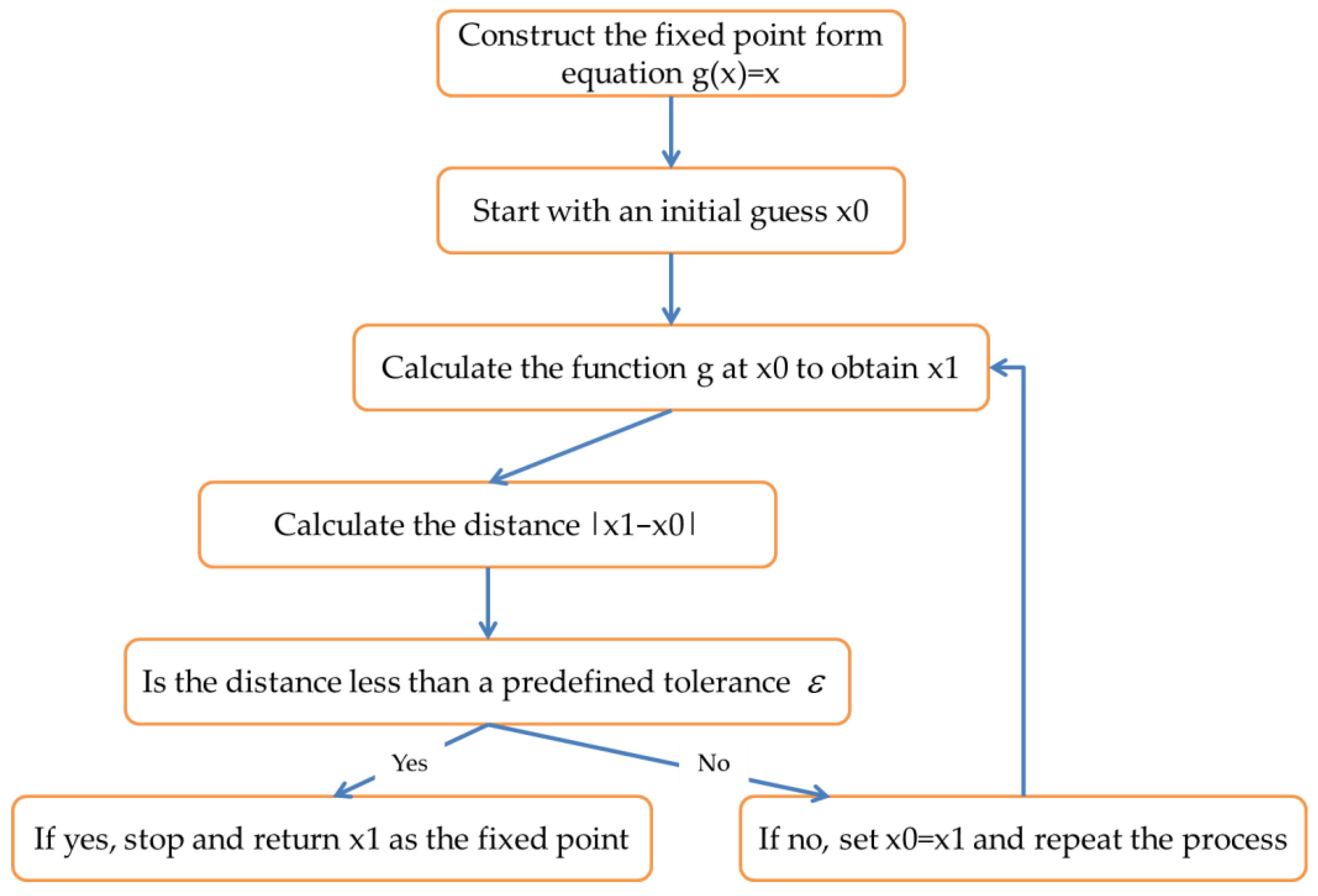
2.2. Unbiased IF Estimation Based Fixed Point of FEO

We consider a special category of signals: linear chirp signals of $f(t)=A{e}^{i\varphi (t)}$, where $\varphi (t)=a_2+b_{2}t+\frac{1}{2}{c}_2{t}^2 and A>0, a_2,b_2,c_2$ are real numbers. For each $\eta$ and $t$,

$$f(\eta +t)=f(t)e^{i[{\varphi }^{\prime }(t)\eta +\frac{1}{2}{\varphi }^{″}(t){\eta }^2]}$$

(11)

According to Equation (3), the STFT of $f(t)$ is derived as [40]

$$\begin{array}{ll}\hfill S_f^g(\omega ,t)& ={\displaystyle {\int }_{ℝ}f}(\xi )\cdot g(\xi -t)\cdot e^{-i\omega (\xi -t)}d\xi \hfill \\ & ={\displaystyle {\int }_{ℝ}f}(\eta +t)\cdot g(\eta )\cdot e^{-i\omega \eta }d\eta \hfill \\ & ={\displaystyle {\int }_{ℝ}f}(t)e^{i[{\varphi }^{\prime }(t)\eta +\frac{{\varphi }^{\prime \prime }(t){\eta }^2}{2}]}\cdot a{e}^{-\frac{{\eta }^2}{b}}\cdot e^{-i\omega \eta }d\eta \hfill \\ & =a\cdot f(t){\displaystyle {\int }_{ℝ}{e}^{(i\frac{{\varphi }^{\prime \prime }(t)}{2}-\frac{1}{b}){\eta }^2}}{e}^{-i\eta (\omega -{\varphi }^{\prime }(t))}d\eta \hfill \\ & =a\cdot f(t){\displaystyle {\int }_{ℝ}{e}^{-u{(\eta +\frac{iv}{2u})}^2}}d\eta \cdot e^{-\frac{v^2}{4u}}\hfill \\ & =a\cdot f(t)\cdot \sqrt{\frac{\pi }{u}}\cdot e^{-\frac{v^2}{4u}}\hfill \end{array}$$

(12)

where $\eta =\xi -t$, $u=\frac{1}{b}-i\frac{{\varphi }^{″}(t)}{2}$, and $v=\omega -{\varphi }^{\prime }(t)$.

Then, the IF estimation of signal $f$ is obtained as

$${\widehat{\omega }}_f(\omega ,t)=\Re \left(\frac{{\partial }_t{S}_f^g}{i{S}_f^g}\right)={\varphi }^{\prime }(t)+\frac{{\left({\varphi }^{″}(t)\right)}^2}{4/b^2+{\left({\varphi }^{″}(t)\right)}^2}\left(\omega -{\varphi }^{\prime }(t)\right)$$

(13)

Therefore,

$$\left|{\widehat{\omega }}_f(\omega ,t)-{\varphi }^{\prime }(t)\right|=\frac{{\left({\varphi }^{″}(t)\right)}^2}{4/b^2+{\left({\varphi }^{″}(t)\right)}^2}\left|\omega -{\varphi }^{\prime }(t)\right|$$

(14)

which clearly shows that the IF estimation ${\widehat{\omega }}_f(\omega ,t)\ne {\varphi }^{\prime }(t)$ as soon as ${\varphi }^{″}(t)\ne 0$, i.e., $c\ne 0$. Furthermore, the deviation between the IF estimation and the true one is positively related to $|{\varphi }^{″}(t)|$. Therefore, ${\widehat{\omega }}_f(\omega ,t)$ cannot be regarded as a good estimation of the IF [41]. To achieve a more accurate IF estimation, the operator defined in Equation (9) has been improved [42]. However, when substituting ${\varphi }^{\prime }(t)$ for the variable $\omega$ in Equation (14), we can obtain ${\widehat{\omega }}_f\left({\varphi }^{\prime }(t),t\right)={\varphi }^{\prime }(t)$. That is to say that the IF of ${\varphi }^{\prime }(t)$ is the fixed point of ${\widehat{\omega }}_f(\omega ,t)$ with respect to frequency $\omega$, which motivates us to use a novel method to represent the IF by combining the fixed-point algorithm with the frequency reassignment operator. Furthermore, the proposed algorithm can mitigate the impact of signal amplitude variations on frequency estimation. Thus, it will also present the IFs of weak components.

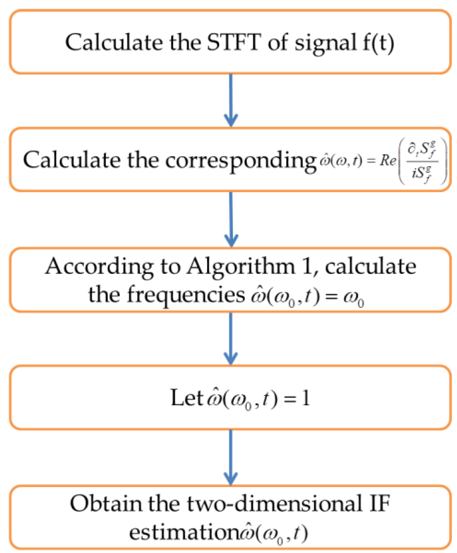
3. The Proposed Algorithm

Based on the above analysis, we can propose a novel method to extract the IF of a chirp signal. It solves a fixed-point equation with the form $F(\omega )=\omega$, where $F(\omega )={\widehat{\omega }}_f(\omega ,t)$ at each time ($t$). This problem is considered as follows: for a given time ($t_0$), find $\omega$ such that ${\widehat{\omega }}_f(\omega ,t_0)=\omega$.

To solve the equation of the extraction of a constant-amplitude linear chirp, we can naturally use the classical fixed-point algorithm, which is as follows: let ${\omega }_0(t_0)$ be an “arbitrary” initial value; ${\omega }_{k+1}(t_0)={\widehat{\omega }}_f({\omega }_k(t_0),t_0)$; the convergence criterion is $\left|{\omega }_{k+1}-{\omega }_k\right|<t_o$; and $t_0$ is fixed, arbitrary, and small.

In order to ensure the convergence of the algorithm, we need to check that for any two consecutive iterations ($k$ and $k+1$), $\left|F({\omega }_{k+1})-F({\omega }_k)\right|<\left|{\omega }_{k+1}-{\omega }_k\right|$. Based on Equation (12), the derivative of $F(\omega )$ with respect to $\omega$ is given by

$$\frac{\partial F(\omega )}{\partial \omega }=\frac{{\left({\varphi }^{″}(t)\right)}^2}{4/b^2+{\left({\varphi }^{″}(t)\right)}^2}$$

(15)

whose absolute value is obviously smaller than $L$ given that $0<L<1$. Since $\frac{\partial F(\omega )}{\partial \omega }$ is independent of $\omega$, $F$ is contractive on $\omega \in \left[{\varphi }^{\prime }(t)-\Delta ,{\varphi }^{\prime }(t)+\Delta \right]$. The corresponding flowcharts of algorithms are displayed in Figure 1 and Figure 2.

4. Experimental Results and Analysis

We use the FSST-based methods [42,43] for comparison. One may give an estimation of the IF as

$${\tilde{\omega }}_i=\underset{j}{\max }FSST({\omega }_j,t_i),0⩽i⩽N-1$$

(16)

The curve $({\tilde{\omega }}_i,t_i),0⩽i⩽N-1$ gives an IF estimation based on the FSST.

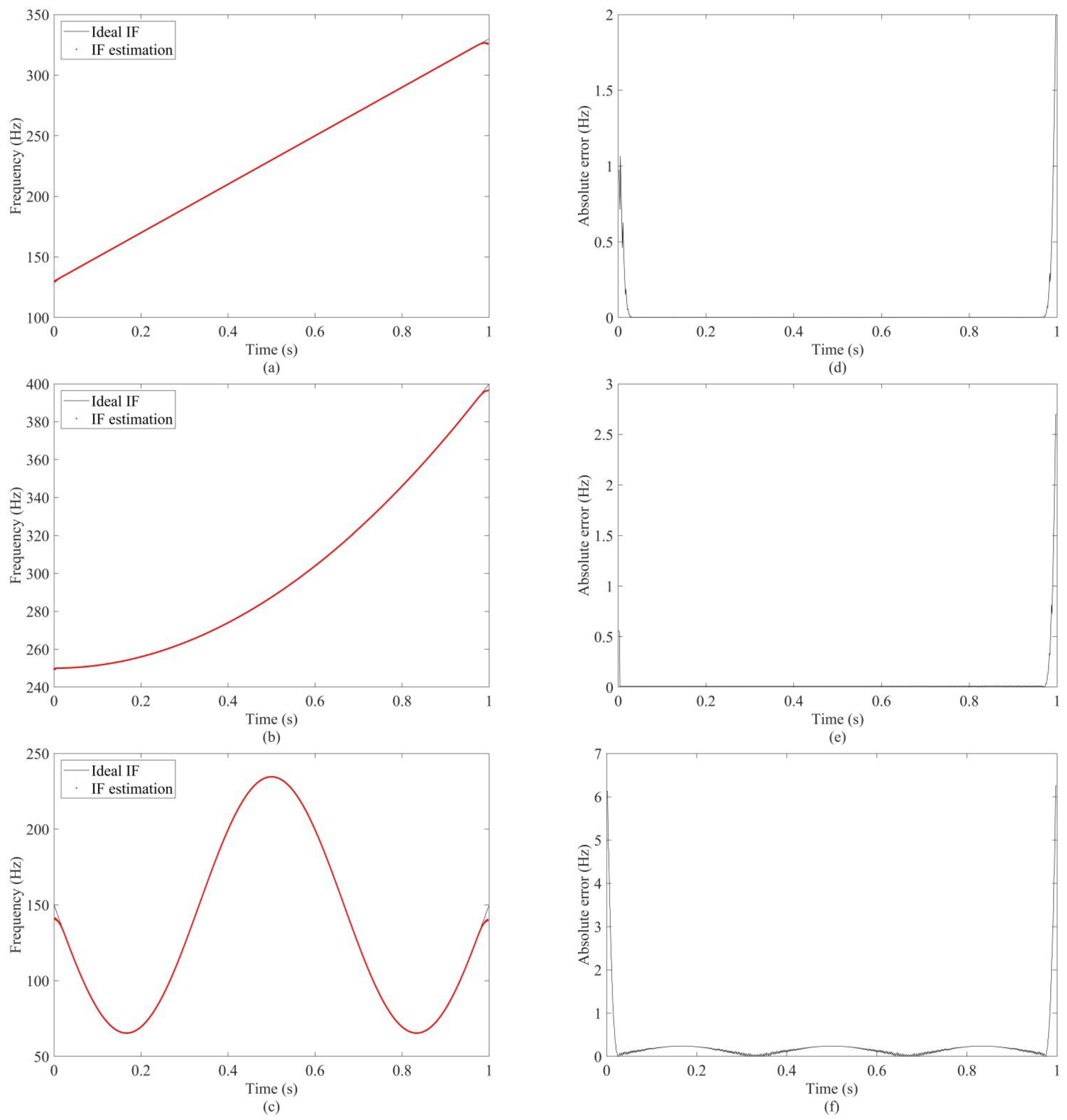
4.1. Single-Component Signal

In order to verify the performance of the proposed method for the extraction of the IF, we employ three mono-component signals with different frequency characters. The three test signals are a linear frequency modulation signal, a three-order polynomial phase signal, and a non-linear phase signal. The corresponding number forms are

$$f_1(t)=e^{i(130t+100t^2)},f_2(t)=e^{i(250t+50t^3)},f_3(t)=e^{i(150t+9cos(3\pi t))}$$

(17)

and the sample interval is $1/1024$ s. Figure 3a–c represent the results of IF estimations using the proposed method. The corresponding absolute errors between the estimations and the ideal IF are shown in Figure 3d–f, and their mean absolute errors are 0.0276, 0.0364, and 0.2411, respectively. From these three noise-free experiments, we directly draw the conclusion that the estimation error obtained using the proposed approach can almost be controlled under the limit value. Furthermore, it is interesting to examine the effectiveness and robustness of the proposed algorithm under noisy circumstances. Herein, we will compare the obtained result and the ideal one using the mean absolute error. We apply different signal-to-noise ratio (SNR) values ranging from 0 to 20 dB. Figure 4a–c display the results achieved using the two methods. The results show the benefits of taking the fixed-point operator into account. It can be observed that the new method is always lower than the FSST, which means that the new algorithm is more accurate and robust than the FSST-based method.

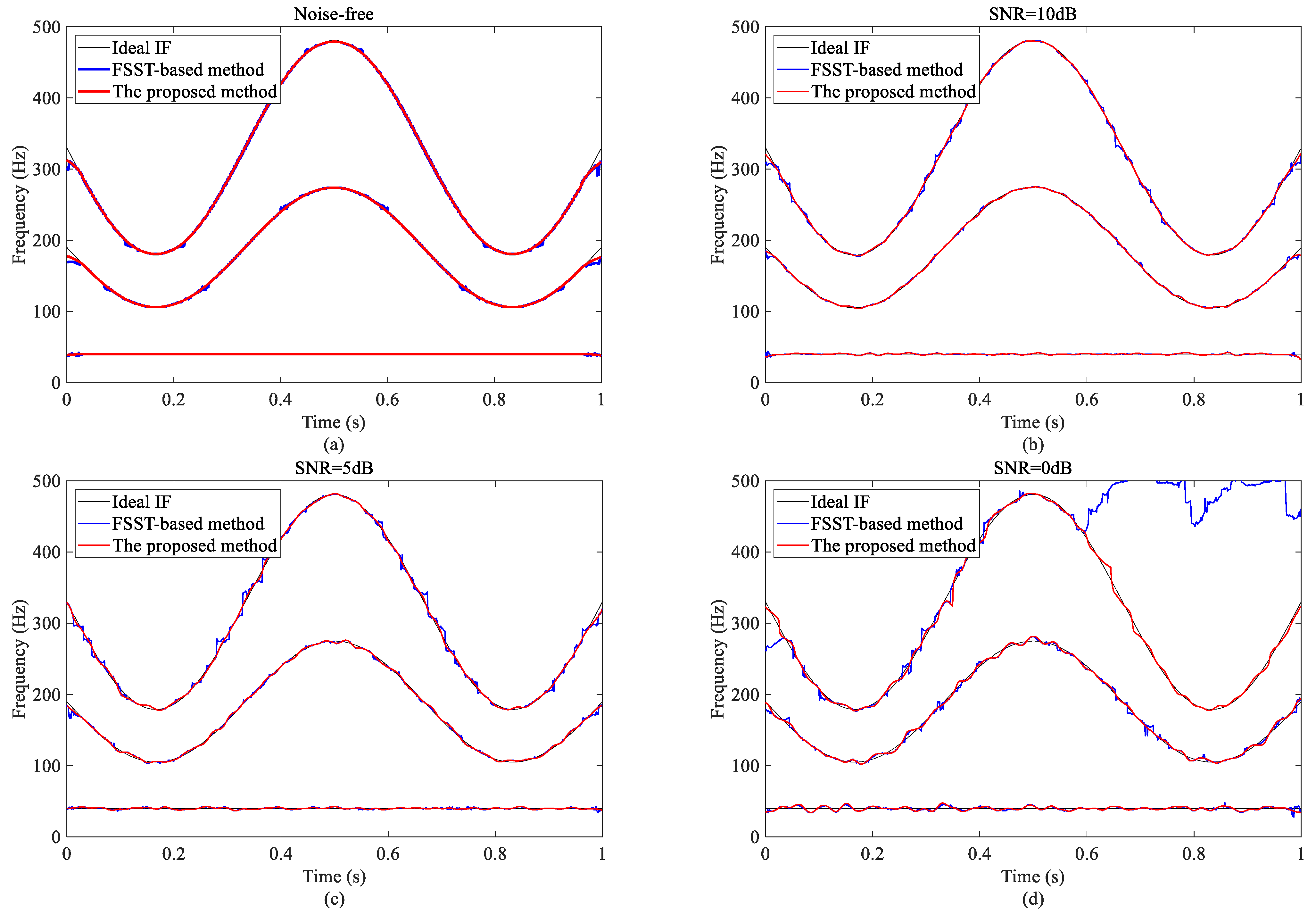
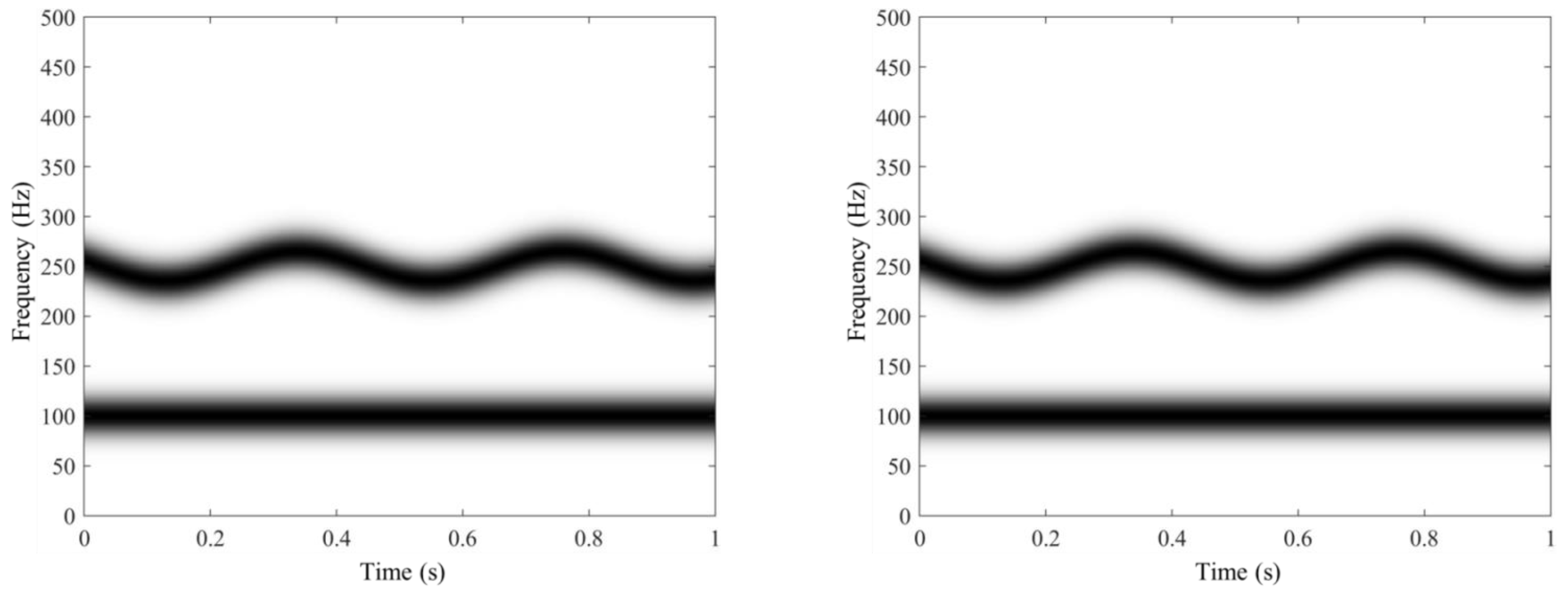
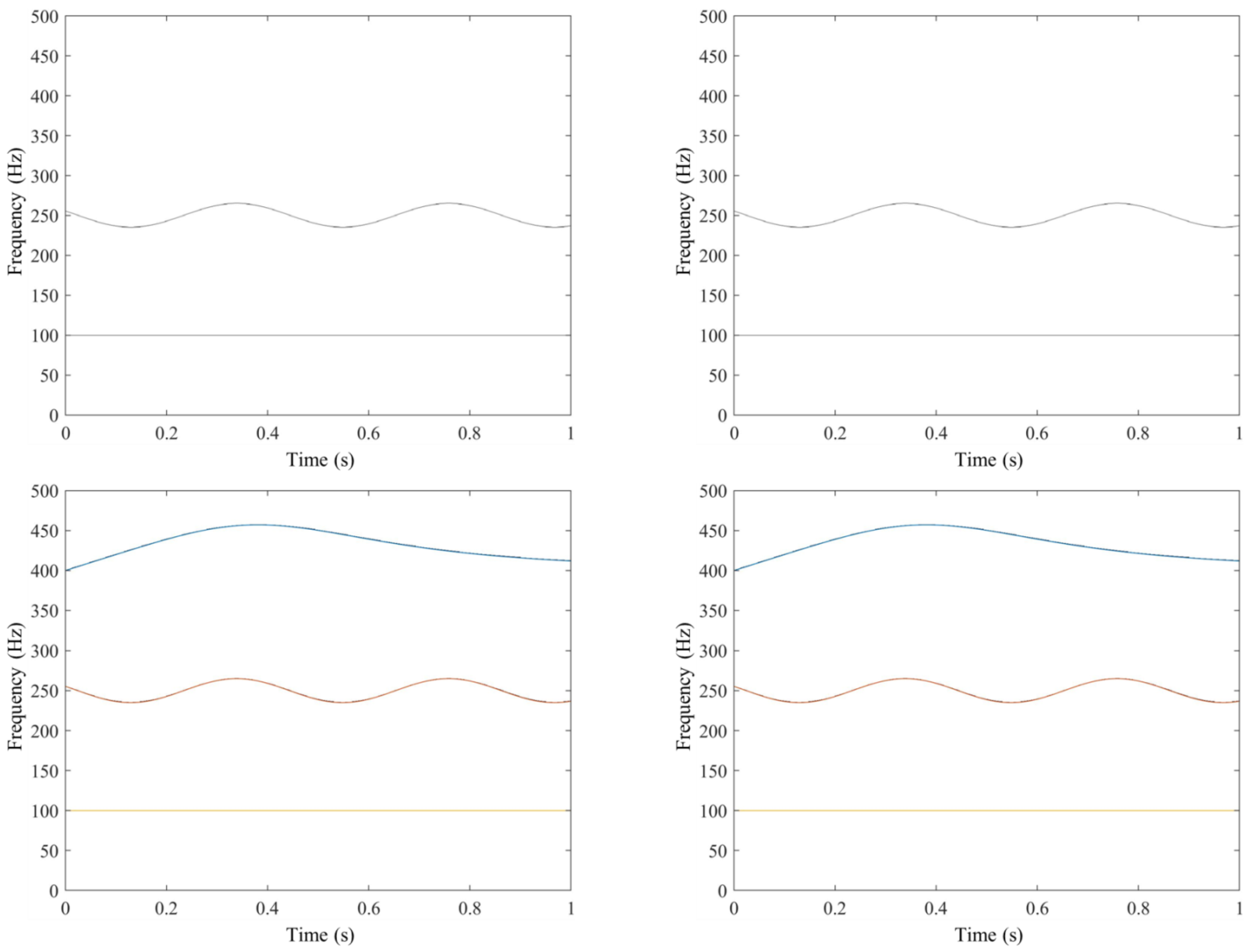
4.2. Multicomponent Signal

Regardless of whether it is for the FSST or for the proposed method, to decompose a multi-component signal into the mono-component modes, the first step is to estimate the IF trajectories corresponding to each mode. Next, the proposed algorithm and the FSST-based method are applied to a multicomponent synthetic signal ($f_4\left(t\right)$) with different levels of noises. Figure 5 illustrates the estimated IF trajectories based on the FSST and the proposed method. It can be seen that, for the high SNR level (Figure 5a), both methods can present correct IF trajectories. However, for the low SNR level (Figure 5c,d), the estimated IF trajectories based on the FSST are untrusted. Although the proposed method results are affected by noise, the IF trajectories of the three modes are still well estimated. Thus, it can be concluded that the IF estimations obtained using the proposed method (the red lines) are smoother and more robust than the FSST (the blue lines). Notably, different from the FSST-based method, the new algorithm is completely adaptive and detects the number of modes in the signal.

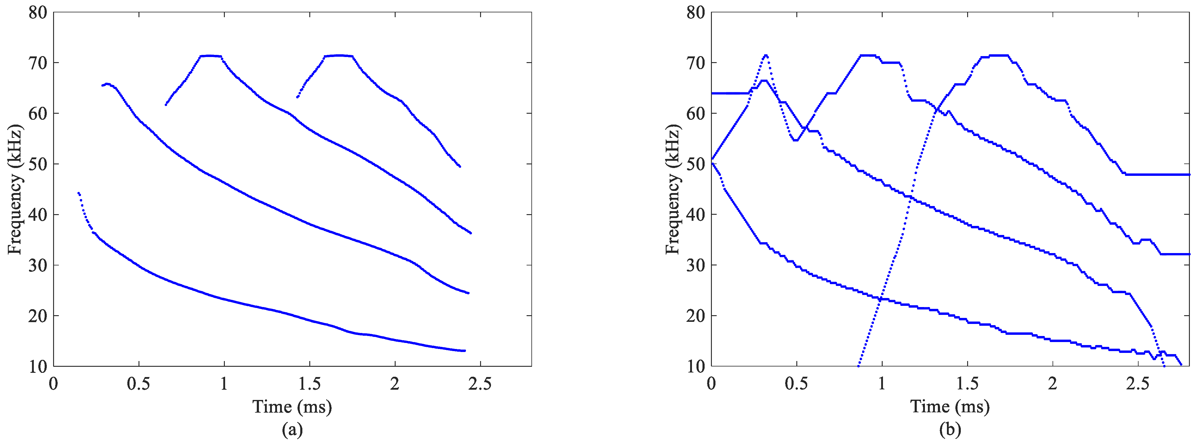
4.3. Bat Echolocation

Finally, we consider a bat echolocation call, which is available at Supplementary Materials. Figure 6 shows the estimated IF trajectories based on the proposed algorithm and the FSST. From Figure 6a, it can be seen that the result based on the proposed method gives a better description of IF trajectories. In Figure 6b, the estimated IF trajectories obtained by the FSST partially overlap with each other. Utilizing the IF trajectories estimated using the result of the proposed method, the mono-component modes are decomposed effectively. Figure 7 displays the four decomposed components. Figure 7e lists the summation of the four modes (the red line) and the original bat signal (the black line). The reconstruction errors are shown in Figure 7f. From the result, it can be observed that the reconstruction errors are small, which means that the estimated TF is comparatively accurate.

4.4. Weak Component Detection

In this section, we utilize two simulated signals to test the performance of the proposed method in weak signal detection and IF extraction. The two signals can be expressed as $s(t)={\displaystyle \sum _{i=1}^3{s}_i}(t)$, where

$$\begin{array}{l}{s}_1=a\cdot sin(2\pi (400t+25\arctan {(2t-1)}^2)),\\ s_2=sin(2\pi (250t+sin(15t))),\\ s_3=sin(2\pi (100t)).\end{array}$$

(18)

The sampling frequency is 1 kHz, and the number of samples is 1000. Herein, we have chosen the STFT and FSST, two representative tools, as the compared methods. The corresponding results are presented in Figure 8. For the two cases where $\mathrm{a}=0.05 \mathrm{o}\mathrm{r} \mathrm{a}=0.001$, the STFT and FSST can show the TF features of $s_2$ and $s_3$ but not $s_1$. The bottom of Figure 8 shows the detected IFs (colored lines) by the proposed algorithm and the theoretical values (black lines). Even though each case has a weak mode with much lower amplitude than the two other modes, the proposed method always has an approximated result. These results verify that the proposed method can be used as an effective tool for IF extraction from the weak components within a signal.

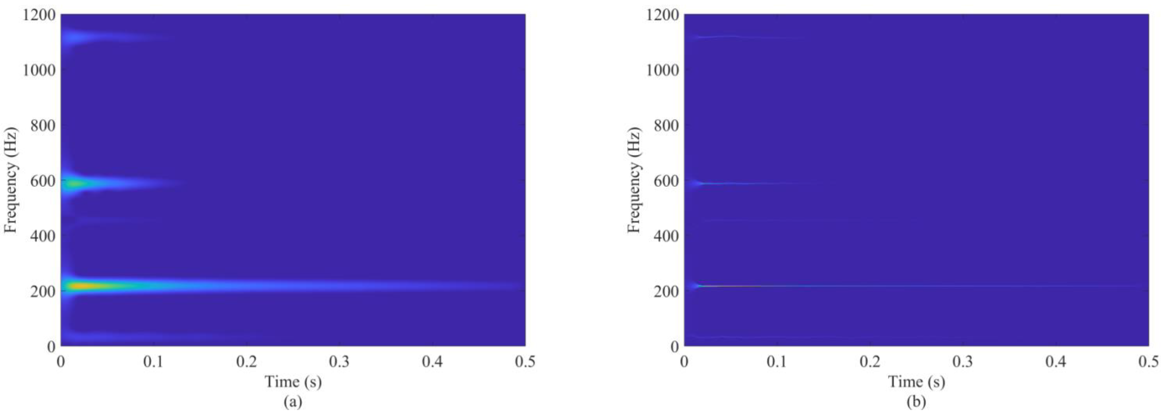
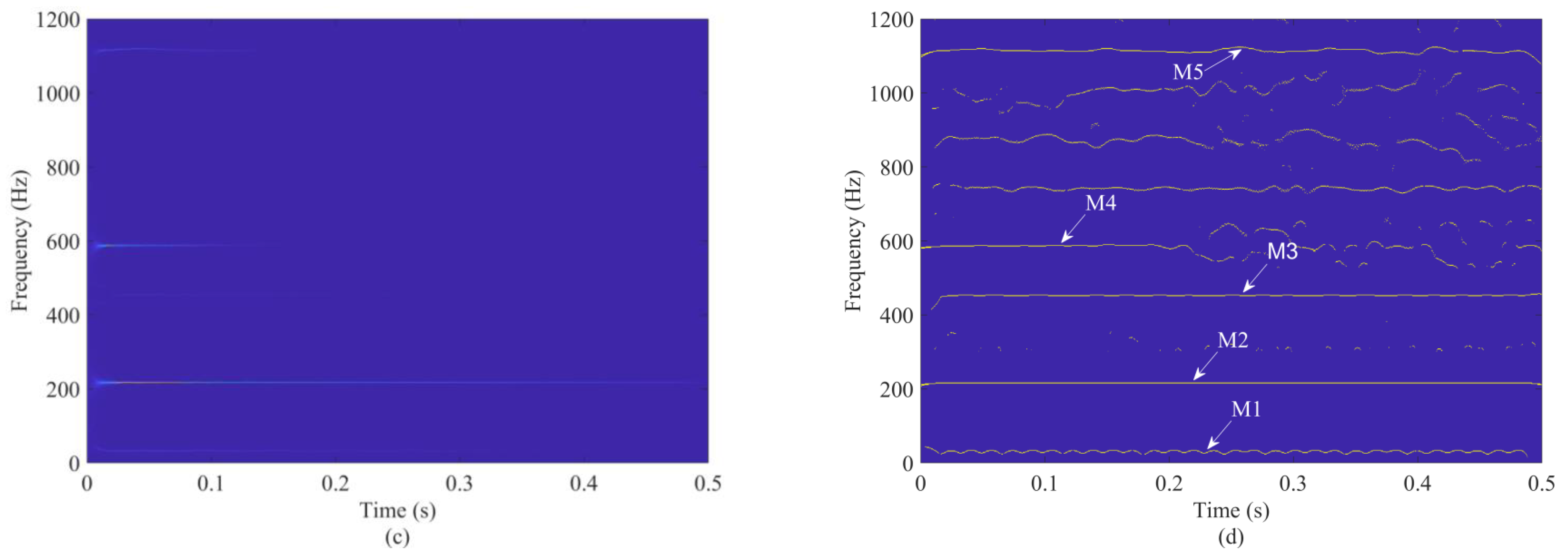
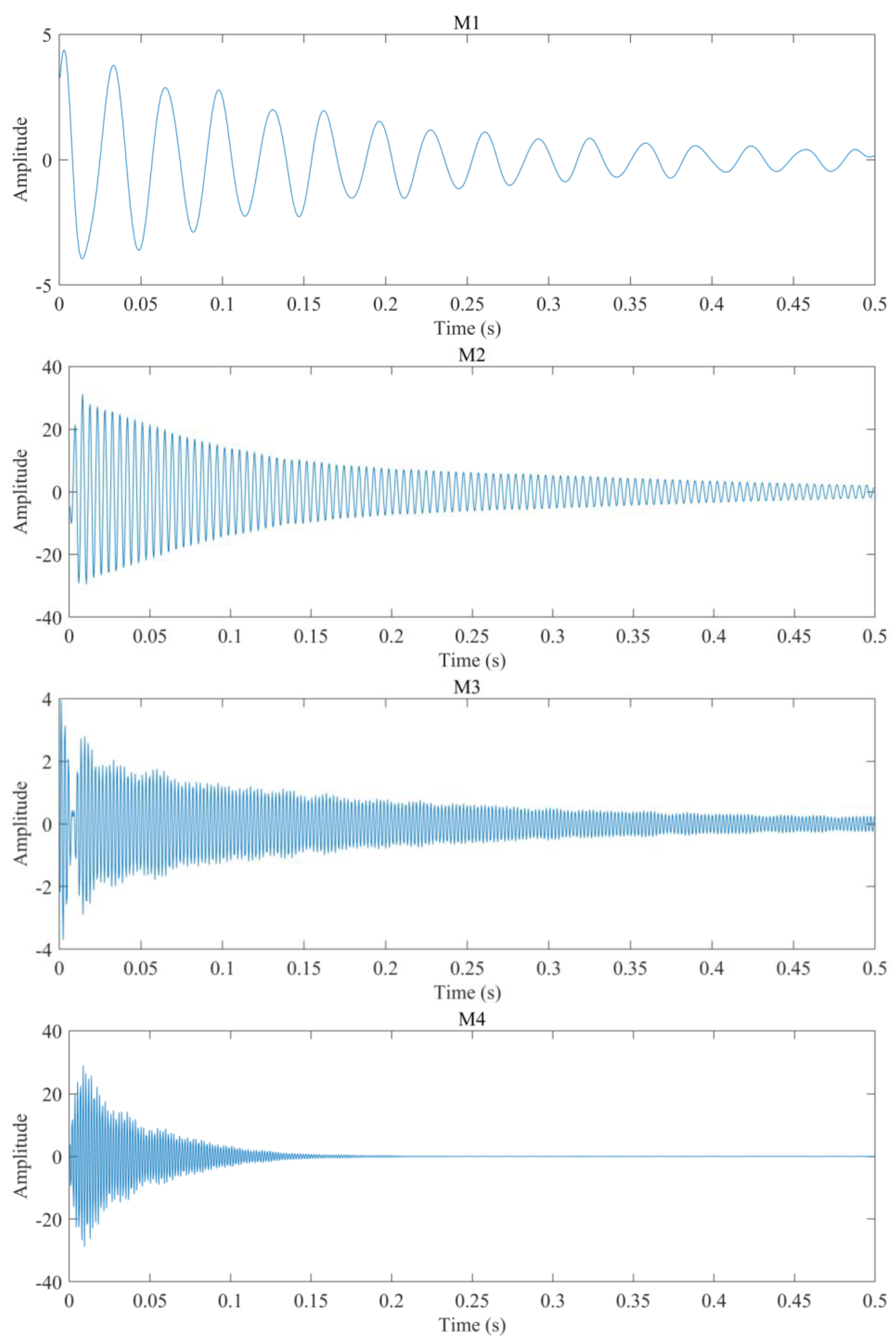
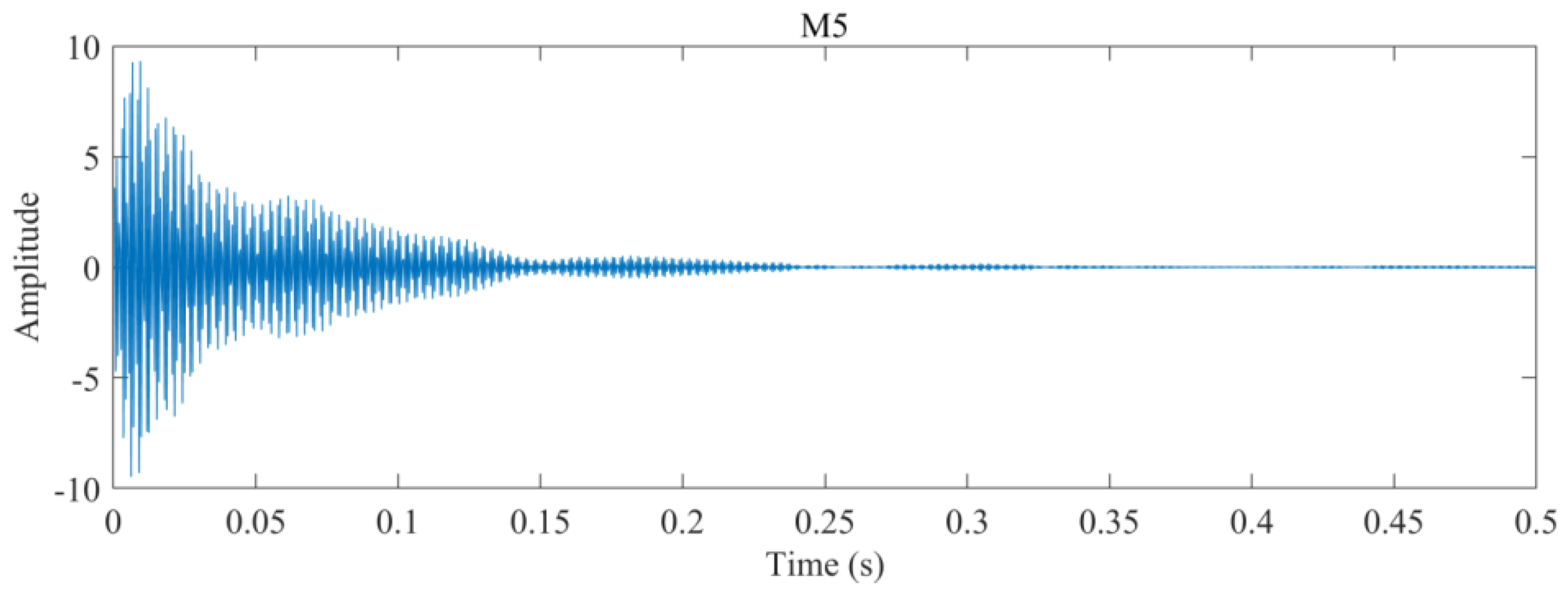
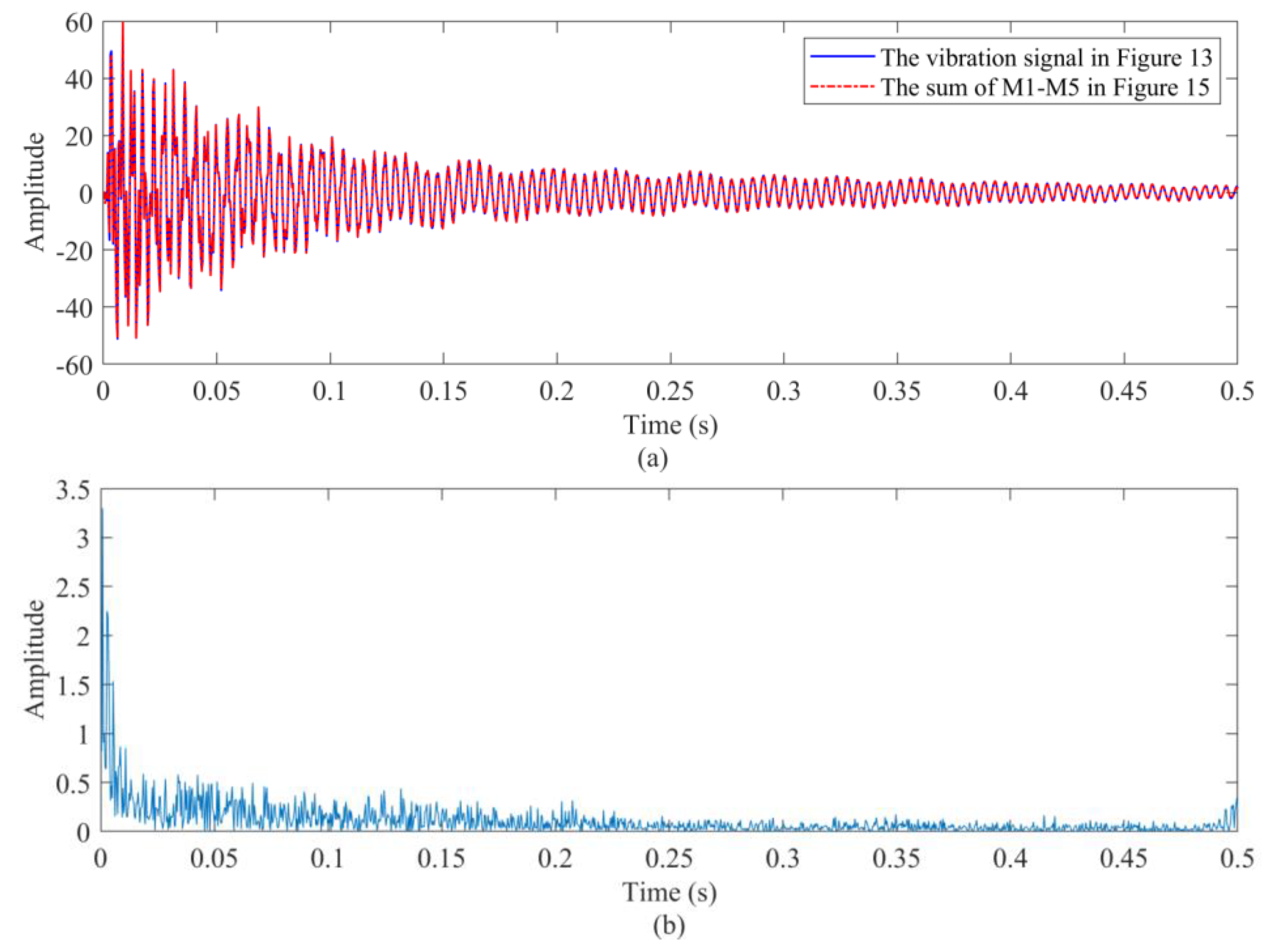
4.5. Vibration Signal

In this section, a vibration signal recorded from a beam excited using a hammer is employed, as shown in Figure 9a. As we know, identifying the parameters of modes is important in structural engineering. In Figure 9b, we can see that the features of the modal signals have some transient properties, and the accurate parameters for each mode are difficult to determine based only on this spectrum. Herein, we use the TFR for the frequency and damping extraction of each mode of the structure.

The corresponding results are shown in Figure 10. In Figure 10a–c, the TF features of weak modes are displayed incompletely and are thus not suitable for retrieving all modes to study the corresponding modal parameters. However, from the result obtained using the proposed method, the IF features of each mode are revealed clearly, as shown in Figure 10d. Therefore, we can obtain the TF localizations to reconstruct each mono-component individually. Figure 11 presents modes M1–M5, which can be used to estimate the frequency and damping parameters conveniently. Based on the proposed method, the amplitudes of the reconstructed results are consistent with Figure 9. From Figure 9b, it can be seen that modes M1 and M3 are with weak energies, which are also well retrieved. Based on the absolute errors (Figure 12b) between the vibration signal and the reconstructed signal (Figure 12a), it can be seen that the proposed method retrieves almost all the components within the vibration signal. In fact, in Figure 10d, there are some frequency features that are not revealed in Figure 9b, which may include a desired signal with weak amplitude. This practical example fully demonstrates the potential of the proposed method.

5. Conclusions

In this paper, we showed that the IF can be extracted using the fixed points of the frequency reassignment operator $\widehat{\omega }(\omega ,t)$ with respect to the variable ω. A novel method based on the fixed-point iteration algorithm was used to adaptively obtain the IF for the chirp-like signals. The numerical experiments verified that the proposed technique has good robustness and high estimation accuracy; does not need the number of modes; and can adaptively detect IFs, even for weak components. It is worth mentioning that the proposed method uses a simple mathematical theory based on the original frequency estimation operator, and it can easily be generalized to other higher-order methods. IFs and other parameters of targets are determined using each mode of a structure. Therefore, how to better extract the IF of each mode and retrieve the corresponding structure needs to be studied more deeply in the future.

References

1. Boashash, B. Estimating and interpreting the instantaneous frequency of a signal. I. Fundamentals. IEEE Proc. 1992, 80, 510–538. [Google Scholar] [CrossRef]
2. Boashash, B. Estimating and interpreting the instantaneous frequency of a signal-Part 2: Algorithms and applications. IEEE Proc. 1992, 80, 540–568. [Google Scholar] [CrossRef]
3. Borovkova, E.I.; Ponomarenko, V.I.; Karavaev, A.S.; Dubinkina, E.S.; Prokhorov, M.D. Method of Extracting the Instantaneous Phases and Frequencies of Respiration from the Signal of a Photoplethysmogram. Mathematics 2023, 11, 4903. [Google Scholar] [CrossRef]
4. Guharaya, S.K.; Thakura, G.S.; Goodmana, F.J.; Rosena, S.L.; Houser, D. Analysis of non-stationary dynamics in the financial system. Econ. Lett. 2013, 121, 454–457. [Google Scholar] [CrossRef]
5. Huang, Y.; Zhang, Q.; Zhong, J.; Chen, Z.; Zhong, S. Parameterized Instantaneous Frequency Estimation Method for Vibration Signal with Nonlinear Frequency Modulation. Machines 2022, 10, 777. [Google Scholar] [CrossRef]
6. Razzaq, H.S.; Hussain, Z.M. Instantaneous Frequency Estimation of FM Signals under Gaussian and Symmetric α-Stable Noise: Deep Learning versus Time–Frequency Analysis. Information 2023, 14, 18. [Google Scholar] [CrossRef]
7. Cohen, L.; Lee, C. Instantaneous frequency and timefrequency distributions. Proc. IEEE Int. Symp. Circuits Syst. 1989, 2, 1231–1234. [Google Scholar]
8. Stankovic, L.; Katkovnik, V. Algorithm for the instantaneous frequency estimation using time-frequency distributions with adaptive window width. IEEE Signal Process. Lett. 1998, 5, 224–227. [Google Scholar] [CrossRef] [PubMed]
9. Iatsenko, D.; McClintock, P.V.E.; Stefanovska, A. Extraction of instantaneous frequencies from ridges in time-frequency representations of signals. Signal Process. 2016, 125, 290–303. [Google Scholar] [CrossRef]
10. Lovell, B.C.; Williamson, R.C. The statistical performance of some instantaneous frequency estimators. IEEE Trans. Signal Process. 1992, 40, 1708–1724. [Google Scholar] [CrossRef]
11. Huang, N.E.; Shen, Z.; Long, S.R.; Wu, M.L.; Shi, H.H.; Zheng, Q.; Yen, N.C.; Tung, C.C.; Liu, H.H. The empirical mode decomposition and hilbert spectrum for nonlinear and nonstationary time series analysis. Proc. R. Soc. Lond. A 1998, 454, 903–995. [Google Scholar] [CrossRef]
12. Huang, N.E.; Wu, Z. A review on Hilbert-Huang transform: Method and its applications to geophysical studies. Rev. Geophys. 2008, 46. [Google Scholar] [CrossRef]
13. Tary, J.B.; Herrera, R.H.; Han, J.J.; van der Baan, M. Spectral estimation–what is new? What is next? Rev. Geophys. 2014, 52, 723–749. [Google Scholar] [CrossRef]
14. Gabor, D. Theory of communication. J. Inst. Electr. Eng. 1946, 93, 429–457. [Google Scholar] [CrossRef]
15. Morlet, J.; Arens, G.; Fourgeau, E.; Glard, D. Wave propagation and sampling theory-Part II: Sampling theory and complex waves. Geophysics 1982, 47, 222–236. [Google Scholar] [CrossRef]
16. Grossmann, A.; Morlet, J. Decomposition of Hardy functions into square integrable wavelets of constant shape. SIAM J. Math. Anal. 1984, 15, 723–736. [Google Scholar] [CrossRef]
17. Stockwell, R.G.; Mansinha, L.; Lowe, R. Localization of the complex spectrum: The S transform. IEEE Trans. Signal Process. 1996, 44, 998–1001. [Google Scholar] [CrossRef]
18. Wignaer, E. On the quantum correction for the rmodynamic equilibrium. Phys. Rev. 1932, 40, 749–759. [Google Scholar] [CrossRef]
19. Ville, J. Theorie et applications de la notion de signal analytique. Cables Trans. 1948, 2A, 61–67. [Google Scholar]
20. Swiercz, E.; Janczak, D.; Konopko, K. Estimation and Classification of NLFM Signals Based on the Time–Chirp Representation. Sensors 2022, 22, 8104. [Google Scholar] [CrossRef]
21. Jurdana, V.; Vrankic, M.; Lopac, N.; Jadav, G.M. Method for Automatic Estimation of Instantaneous Frequency and Group Delay in Time–Frequency Distributions with Application in EEG Seizure Signals Analysis. Sensors 2023, 23, 4680. [Google Scholar] [CrossRef] [PubMed]
22. Delprat, N.; Escudie, B.; Guillemain, P.; Kronland-Martinet, R.; Tchamitchian, P.; Torresani, B. Asymptotic wavelet and Gabor analysis: Extraction of instantaneous frequencies. IEEE Trans. Inf. Theory 1992, 38, 644–664. [Google Scholar] [CrossRef]
23. Wu, H.T.; Chan, Y.H.; Lin, Y.T.; Yeh, Y.H. Using synchrosqueezing transform to discover breathing dynamics from ECG signals. Appl. Comput. Harmon. Anal. 2014, 36, 354–459. [Google Scholar] [CrossRef]
24. Sandoval, S.; De Leon, P.L. Recasting the (Synchrosqueezed) Short-Time Fourier Transform as an Instantaneous Spectrum. Entropy 2022, 24, 518. [Google Scholar] [CrossRef] [PubMed]
25. Auger, F.; Flandrin, P. Improving the readability of time-frequency and time-scale representations by the reassignment method. IEEE Trans. Signal Process. 1995, 43, 1068–1089. [Google Scholar] [CrossRef]
26. Daubechies, I.; Lu, J.; Wu, H. Synchrosqueezed wavelet transforms: An empirical mode decomposition-like tool. Appl. Comput. Harmon. Anal. 2011, 30, 243–261. [Google Scholar] [CrossRef]
27. Oberlin, T.; Meignen, S.; Perrier, V. Second-order synchrosqueezing transform or invertible reassignment? Towards ideal time-frequency representations. IEEE Trans. Signal Process. 2015, 63, 1335–1344. [Google Scholar] [CrossRef]
28. Behera, R.; Meignen, S.; Oberlin, T. Theoretical analysis of the second-order synchrosqueezing transform. Appl. Comput. Harmon. Anal. 2018, 45, 379–404. [Google Scholar] [CrossRef]
29. Oberlin, T.; Meignen, S. The second-order wavelet synchrosqueezing transform. In Proceedings of the 2017 IEEE International Conference on Acoustics, Speech and Signal Processing (ICASSP), New Orleans, LA, USA, 5–9 March 2017. [Google Scholar]
30. Han, B.; Zhou, Y.; Yu, G. Second-order synchroextracting wavelet transform for nonstationary signal analysis of rotating machinery. Signal Process. 2021, 186, 108123. [Google Scholar] [CrossRef]
31. Yu, G.; Lin, T. Second-order transient-extracting transform for the analysis of impulsive-like signals. Mech. Syst. Signal Process. 2021, 147, 107069. [Google Scholar] [CrossRef]
32. Pham, D.; Meignen, S. High-order synchrosqueezing transform for multicomponent signals analysis—With an application to gravitational-wave signal. IEEE Trans. Signal Process. 2017, 65, 3168–3178. [Google Scholar] [CrossRef]
33. Lv, S.; Lv, Y.; Yuan, R.; Li, H. High-order synchroextracting transform for characterizing signals with strong AM-FM features and its application in mechanical fault diagnosis. Mech. Syst. Signal Process. 2022, 172, 108959. [Google Scholar] [CrossRef]
34. Wang, S.; Chen, X.; Cai, G.; Chen, B.; Li, X.; He, Z. Matching demodulation transform and synchrosqueezing in time-frequency analysis. IEEE Trans. Signal Process. 2014, 62, 69–84. [Google Scholar] [CrossRef]
35. Miao, Y.; Sun, H.; Qi, J. Synchro-Compensating Chirplet Transform. IEEE Signal Process. Lett. 2018, 25, 1413–1417. [Google Scholar] [CrossRef]
36. Miao, Y.C.; Qasem, Z.A.H.; Li, Y.S. Adaptive directional ridge prediction tracker for instantaneous frequency estimation. Signal Process. 2023, 209, 109035. [Google Scholar] [CrossRef]
37. Mandel, L. Interpretation of instantaneous frequency. Am. J. Phys. 1974, 42, 840–846. [Google Scholar] [CrossRef]
38. Stanković, L.; Djurović, I.; Stanković, S.; Simeunović, M.; Djukanović, S.; Daković, M. Instantaneous frequency in time–frequency analysis: Enhanced concepts and performance of estimation algorithms. Digit. Signal Process. 2014, 35, 1–13. [Google Scholar] [CrossRef]
39. Fitz, K.R.; Fulop, S.A. A unified theory of time-frequency reassignment. arXiv 2009, arXiv:0903.3080. [Google Scholar]
40. Li, Z.; Gao, J.; Li, H.; Zhang, Z.; Liu, N.; Zhu, X. Synchroextracting transform: The theory analysis and comparisons with the synchrosqueezing transform. Signal Process. 2020, 166, 107243. [Google Scholar] [CrossRef]
41. Auger, F.; Chassande-Mottin, E.; Flandrin, P. On phasemagnitude relationships in the short-time Fourier transform. IEEE Signal Process. Lett. 2012, 19, 267–270. [Google Scholar] [CrossRef]
42. Meignen, S.; Pham, D.; Mclaughlin, S. On demodulation, ridge detection and synchrosqueezing for multicomponent signals. IEEE Trans. Signal Process. 2017, 65, 2093–2103. [Google Scholar] [CrossRef]
43. Oberlin, T.; Meignen, S.; Perrier, V. The Fourier-based synchrosqueezing transform. In Proceedings of the 2014 IEEE International Conference on Acoustics, Speech and Signal Processing, Florence, Italy, 4–9 May 2014; pp. 315–319. [Google Scholar]
Figure 1. The flowchart of algorithm 1.
Remotesensing 16 01412 g001
Figure 2. The flowchart of algorithm 2.
Remotesensing 16 01412 g002
Figure 3. The estimation of the IF using the proposed algorithm for the (a) f 1 ( t ) , (b) f 2 ( t ) , and (c) f 3 ( t ) . The corresponding absolute errors of (d) f 1 ( t ) , (e) f 2 ( t ) , and (f) f 3 ( t ) , respectively.
Remotesensing 16 01412 g003
Figure 4. A comparison of the FSST-based method and the proposed method using signals with different noise levels: (a) f 1 ( t ) , (b) f 2 ( t ) , and (c) f 3 ( t ) .
Remotesensing 16 01412 g004
Figure 5. A multi-component example. The comparisons of IF estimation obtained by the proposed method and FSST-based method under different noise levels: (a) noise-free, (b) 10 dB, (c) 5 dB, and (d) 0 dB.
Remotesensing 16 01412 g005
Figure 6. Extracted IFs of a bat echolocation call calculated using (a) the proposed method and (b) the FSST-based method.
Remotesensing 16 01412 g006
Figure 7. The reconstruction of the bat echolocation call. (ad) The four corresponding modes, (e) the original signal (black) and the reconstructed signal (red), and (f) the error between the reconstructed signal and the original signal.
Remotesensing 16 01412 g007aRemotesensing 16 01412 g007b
Figure 8. The comparison results of case 1 where a = 0.05 (top) and case 2 where a = 0.001 . From (top) to (bottom): STFT, FSST, and the proposed algorithm.
Remotesensing 16 01412 g008aRemotesensing 16 01412 g008b
Figure 9. The tested vibration signal (a) and its spectrum (b).
Remotesensing 16 01412 g009aRemotesensing 16 01412 g009b
Figure 10. The TFRs obtained using the (a) STFT, (b) FSST, and (c) SET, and the detection result obtained using the proposed method (d).
Remotesensing 16 01412 g010aRemotesensing 16 01412 g010b
Figure 11. The reconstructed modes M1—M5.
Remotesensing 16 01412 g011aRemotesensing 16 01412 g011b
Figure 12. (a) The sum of M1—M5 and (b) the absolute errors.
Remotesensing 16 01412 g012
Disclaimer/Publisher’s Note: The statements, opinions and data contained in all publications are solely those of the individual author(s) and contributor(s) and not of MDPI and/or the editor(s). MDPI and/or the editor(s) disclaim responsibility for any injury to people or property resulting from any ideas, methods, instructions or products referred to in the content.