Abstract
Integrated crop–livestock systems (ICLS) are among the main viable strategies for sustainable agricultural production. Mapping these systems is crucial for monitoring land use changes in Brazil, playing a significant role in promoting sustainable agricultural production. Due to the highly dynamic nature of ICLS management, mapping them is a challenging task. The main objective of this research was to develop a method for mapping ICLS using deep learning algorithms applied on Satellite Image Time Series (SITS) data cubes, which consist of Sentinel-2 (S2) and PlanetScope (PS) satellite images, as well as data fused (DF) from both sensors. This study focused on two Brazilian states with varying landscapes and field sizes. Targeting ICLS, field data were combined with S2 and PS data to build land use and land cover classification models for three sequential agricultural years (2018/2019, 2019/2020, and 2020/2021). We tested three experimental settings to assess the classification performance using S2, PS, and DF data cubes. The test classification algorithms included Random Forest (RF), Temporal Convolutional Neural Network (TempCNN), Residual Network (ResNet), and a Lightweight Temporal Attention Encoder (L-TAE), with the latter incorporating an attention-based model, fusing S2 and PS within the temporal encoders. Experimental results did not show statistically significant differences between the three data sources for both study areas. Nevertheless, the TempCNN outperformed the other classifiers with an overall accuracy above 90% and an F1-Score of 86.6% for the ICLS class. By selecting the best models, we generated annual ICLS maps, including their surrounding landscapes. This study demonstrated the potential of deep learning algorithms and SITS to successfully map dynamic agricultural systems.
1. Introduction
Integrated crop–livestock systems (ICLS) are designed in a way that the integration between crop and animal components results in a synergistic relationship that increases diversity within an agroecosystem [1]. The main components of an ICLS are arranged in space and time in a way that they can be managed simultaneously or separately, in rotation or succession. These systems employ sustainable practices to increase productivity and diversify land use, thereby contributing to meeting the food demand of a growing global population. Consequently, they are aligned with the United Nation Sustainable Development Goals (SDGs) [2] related to food security [3], climate change mitigation [4,5], and land conservation [6]. ICLS promote several environmental and agricultural benefits, including efficient nutrient cycling, enhanced soil fertility and structure, recovery of degraded pastures, reduced plant diseases and pest incidents, reduced weeds, accumulation of biomass and organic matter in the soil, and reduction of marketing risks [3,7]. ICLS worldwide adopt a diverse array of crops and livestock species. Their selection depends upon regional factors, such as the animal species, farmers’ goals, available technology, economic and market aspects, and climatic characteristics of the region [7]. Garrett et al. [8] listed several countries that adopt commercial integrated systems on a larger scale. Over the last decade, Brazil has been developing a national policy of incentives to implement integrated production systems, driven mainly by the Plan for Low Carbon Emissions in Agriculture [9]. To assess the successful implementation of these systems, it is essential to develop efficient methods for mapping and monitoring ICLS. This will enable the generation of detailed and timely information on the progress and spatial distribution of integrated systems required by organizations related to the sector or governments.
Dense satellite image time series (SITS) has already been successfully used to map dynamic agricultural areas [10,11,12]. Manabe et al. [13] used Moderate Resolution Imaging Spectroradiometer (MODIS)-based Enhanced Vegetation Index (EVI) time series and Time-Weighted Dynamic Time Warping (TWDWT) to map ICLS in Mato Grosso, one of the most important agricultural producers among the Brazilian states. In that study, the authors encouraged future studies to integrate images with higher spatial resolution to more accurately match the size of crop fields. Similarly, Kuchler et al. [14] used the Random Forest (RF) classifier and MODIS products for the same classification purpose and recommended using images with higher spatial resolution obtained by multi-sensor fusion. Kuchler et al. [14] also suggested testing new machine learning algorithms that can better account for the temporal information required for detecting patterns in highly dynamic targets such as ICLS. In addition, Toro et al. [15] investigated the application of deep learning algorithms on Sentinel-1 (S1) and Sentinel-2 (S2) time series to map ICLS early in the season. Despite S2 data generating the best mapping results, Toro et al. [15] suggested analyses over multiple years and the use of other deep learning networks more specialized in learning spectro-temporal patterns. All previous works emphasized the difficulty of mapping ICLS due to their complexity and heterogeneity.
The improved spatial and temporal resolution of SITS, such as the S2 satellites from the ESA’s Copernicus program or the CubeSats PlanetScope (PS) nanosatellite constellation [16], allows mapping land use and land cover (LULC) with higher details at a low cost. Important research efforts have been dedicated to developing methods to fuse data obtained by several sensors with different characteristics [17]. Sadeh et al. [18] introduced a new method for fusing time series of cloud-free images from S2 and PS to overcome radiometric inconsistencies of the PS images. To successfully estimate the leaf area index in wheat fields, the authors created a consistent series of daily 3 m images (red, green, blue (RGB), and near-infrared (NIR) bands) through data interpolating, resampling S2 images to 3 m and fusing the images by averaging each pair of bands coming from S2 and PS. The reported PS radiometric inconsistencies refer to variations in cross-sensor values of the PlanetScope constellations and the overlapping of their RGB bands, which may interfere with the calculation of spectral indices and classification accuracy results [19]. Recently, Ofori-Ampofo et al. [20] and Garnot et al. [21] demonstrated the advantages of fusing S1 and S2 using deep learning and four fusion strategies.
Motivated by the need to map sustainable agricultural production areas with ICLS and enhance their monitoring, this research aims to demonstrate an end-to-end workflow for mapping ICLS using existing state-of-the-art techniques for data fusion and deep learning algorithms applied to SITS. The RF classifier was used as a baseline for this research since it was tested in previous works for ICLS mapping [14,15]. In addition, we used three deep learning architectures designed to work with SITS; namely, 1D convolutional neural networks, represented in this research by Temporal Convolutional Neural Network (TempCNN) [22], Residual Network (ResNet) [23], and an attention-based model, called Lightweight Temporal Attention Encoder (L-TAE) [24]. We tested two methods for the fusion of S2 and PS data. The main idea behind fusing S2 and PS data was to leverage their distinct characteristics and obtain advantages in terms of spectral, temporal, and spatial resolutions. The first method adapted the fusion methodology developed by Sadeh et al. [18], and generated a regular time series with a 10-day interval and 3 m of spatial resolution. The second method involved fusing the same pre-processed images from S2 and PS inside the temporal encoders of the L-TAE architecture.
The main objective of this research was to develop a method for mapping ICLS fields using deep learning applied to data cubes obtained from the fusion of S2 and PS time series. The proposed method was tested in two different regions of Brazil in three agricultural years (2018/2019, 2019/2020, and 2020/2021). To investigate the benefits of data fusion, we assessed three scenarios considering different sources of data: S2, PS, and data fusion (DF) from both sources. For each scenario, we generated data cubes designed to be free of gaps or missing data, and we compared their performance using four different classification algorithms.
2. Materials and Methods
2.1. Study Area
The study area covers two regions of Brazil that present ICLS and other land uses with different management practices (Figure 1). Study Area 1 (SA1) is located in the municipality of Caiuá, west of the São Paulo State, covering approximately 7300 hectares. Study Area 2 (SA2) is located in the municipalities of Santa Carmem and Sinop, in the north-central region of the Mato Grosso State, covering approximately 49,200 hectares. The study areas are located in different biomes since SA1 belongs to the Atlantic Forest biome and SA2 to the Cerrado biome (Brazilian savannah).
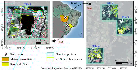
Figure 1.
Location of Study Area 1 (SA1) and Study Area 2 (SA2) in different Brazilian states and the four tiles from the Planet Scope image grid used in this research.
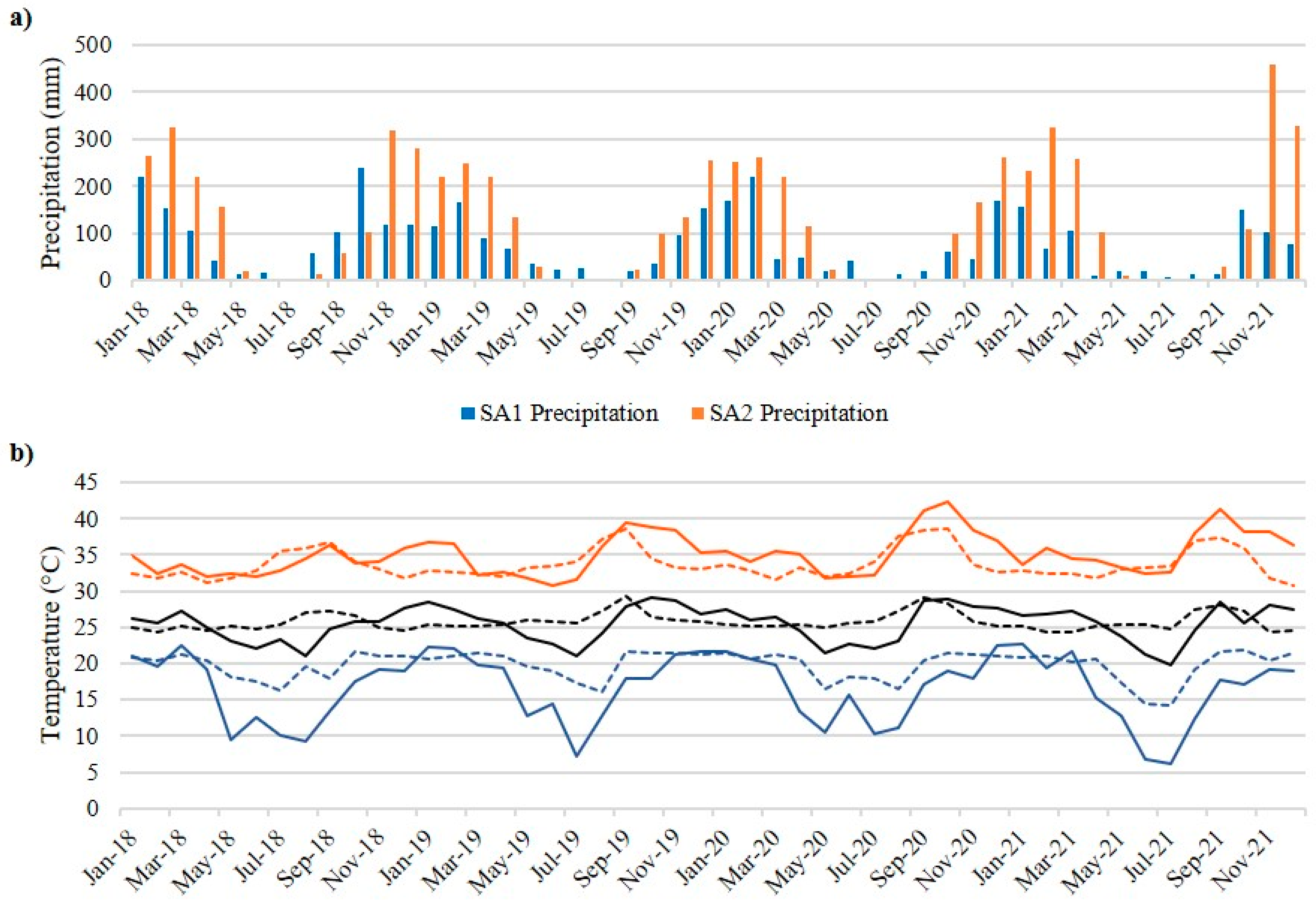
SA1 has fields with small to medium parcels (mean size of 1.45 hectares), with a diversity of crops and a predominance of smallholders. According to the Köppen classification [25], SA1 is under a tropical savanna climate with a rainy summer and dry winter (i.e., June–August). Mean annual precipitation varies between 1200 mm and 1400 mm, and the mean daily temperature is equal to 24.1 °C (Figure 2).
The landscape of SA2 is composed of large-scale parcels (mean size of 11.30 hectares). SA2 is widely known for its high grain production, composed mainly of soybean and corn, where there is also an intensification of land use with the adoption of double crops [26] and improvement in the condition of pastures [27]. SA2 is situated in a tropical wet climate (short dry season) [25], with an average annual precipitation between 1800 and 2300 mm, while the mean daily temperature is equal to 26.2 °C (Figure 2).
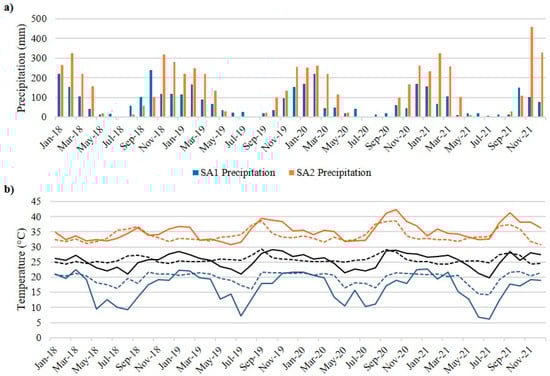
Figure 2.
Monthly precipitation (a) and temperature (b) data obtained from the ECMWF (European Center for Medium-Range Weather Forecasts)/Copernicus Climate Change Service [28], considering the years investigated (2018 to 2021) for SA1 and SA2.
Figure 2.
Monthly precipitation (a) and temperature (b) data obtained from the ECMWF (European Center for Medium-Range Weather Forecasts)/Copernicus Climate Change Service [28], considering the years investigated (2018 to 2021) for SA1 and SA2.
2.2. ICLS Ground Reference Data
We conducted field campaigns for the three agricultural years under study (2018/2019, 2019/2020, 2020/2021). The agricultural year for the study areas starts in September and ends in August of the following year [29]. During the field campaigns, we used a random sampling strategy to collect ground-level data. Additionally, we interviewed farmers to gather insights into the implemented agricultural management and crop rotation practices. These data were fundamental for building our dataset (see Section 2.5), which was later used for training and validating the classification models.
Two main types of ICLS management strategies were observed, namely annual and multi-annual systems. Similar management strategies have been reported by Gil et al. [30], Manabe et al. [13], and Kuchler et al. [14]. The selection of the management strategy depends mainly on the agricultural practices adopted by the farmers and fluctuations in input and output prices in the market [30].
Two main crop seasons exist in Brazil: the summer season and the winter season. The ICLS follow an annual system strategy that is based on crop–pasture succession. All crop management activities within a field are carried out in the same agricultural year and reiterated annually. Soybeans are typically grown as the first crop in the summer, followed by pastures in the winter. Depending on the region’s rainfall pattern, pastures can be cultivated together with mixed species of grasses, leading to land use and other resources optimization throughout the year (e.g., sunlight, biomass production, fertilizers, machinery). Grasses of the genus Urochloa (Brachiaria) are preferentially sown simultaneously with other grass species with a faster vegetative development (corn, millet, or sorghum). The grasses with slower vegetative growth will become established after harvesting or grazing fast-growing grasses. Multi-annual integrated systems are based on crop and livestock succession or rotation, where the fields are managed for more than a year. For a single field, a crop season will be followed by more than two seasons with pastures. The farmers decide to rotate the fields with crop and livestock within the farm considering the spatial and temporal distribution of the fields within the management time interval adopted by the farmer (e.g., 2 years). This type of system is desired mainly for the recovery of pastures since the introduction of crops will provide fertility to the soil.
Based on data collected in the field campaigns and reports from previous studies [13,14], our method for mapping ICLS considers the time interval of one agricultural year. Since our analysis comprises three agricultural years and considering that transitions between crops and pastures inside a single field always occur within an agricultural year, both the annual and multi-annual ICLS management strategies could be identified by the annual mappings.
SA1 has a high diversity in the following LULC classes: Cultivated pasture, Eucalyptus, Forest, ICLS (soybean/millet + brachiaria, soybean/sorghum + brachiaria, and soybean/corn + brachiaria), Pasture consortium (mix of corn + brachiaria, millet + brachiaria, or sorghum + brachiaria), Natural vegetation and wet areas, Perennial crops (annatto, coconut, mango, citrus, acerola, and papaya), Semi-perennial crops (cassava, sugarcane, and Napier grass to make silage), and Others (buildings, roads, and bare soil).
SA2 has a rather homogeneous agricultural pattern and LULC classes: Cultivated pasture, Double crop (soybean/corn, soybean/millet, and soybean/crotalaria), Forest, ICLS (soybean/brachiaria, soybean/cowpeas + brachiaria, soybean/corn + brachiaria, and soybean/millet + brachiaria), Water, and Others (buildings, roads, and bare soil).
2.3. Description of Satellite Data
We used multitemporal images from S2 and PS for the same period of three agricultural years (2018/2019, 2019/2020, 2020/2021) corresponding to the ground reference data timeline. Since our approach uses SITS, data download and some pre-processing steps of S2 were automated through the sen2r package [31]. Using this package, we first downloaded all Level-1C (top of atmosphere (TOA) reflectance) products with a cloud cover of up to 60% and applied the Sen2Cor algorithm for atmospheric correction, converting all products to Level-2A (bottom of atmosphere (BOA) reflectance) resampled to 10 m. Additionally, we applied a cloud and cloud shadow mask to the images using the Scene Classification product of the Sen2Cor algorithm. The atmospheric bands were discarded from the analysis. A total number of 311 S2 images was used for SA1 and 497 for SA2.
Multispectral PS images were acquired from the Planet Labs PBC (Public Benefit Corporation)’s commercial representative platform in Brazil. We selected cloud-free images from the Planet Surface Reflectance product [32]. For SA2, we accounted for dense clouds during the cloudiest months (November to March) and utilized the Usable Data Mask product to mask out clouds and cloud shadows. For PS images, a total number of 900 images were used for SA1 and 2324 for SA2.
2.4. Pre-Processing Satellite Images and Data Fusion
Data pre-processing aimed at obtaining Earth Observation (EO) data cubes which represents multidimensional arrays [33]. The use of EO data cubes, regular in time and space and without missing values, makes operations involving machine learning algorithms easier since they improve multi-data comparability by following a consistent data pattern [34].
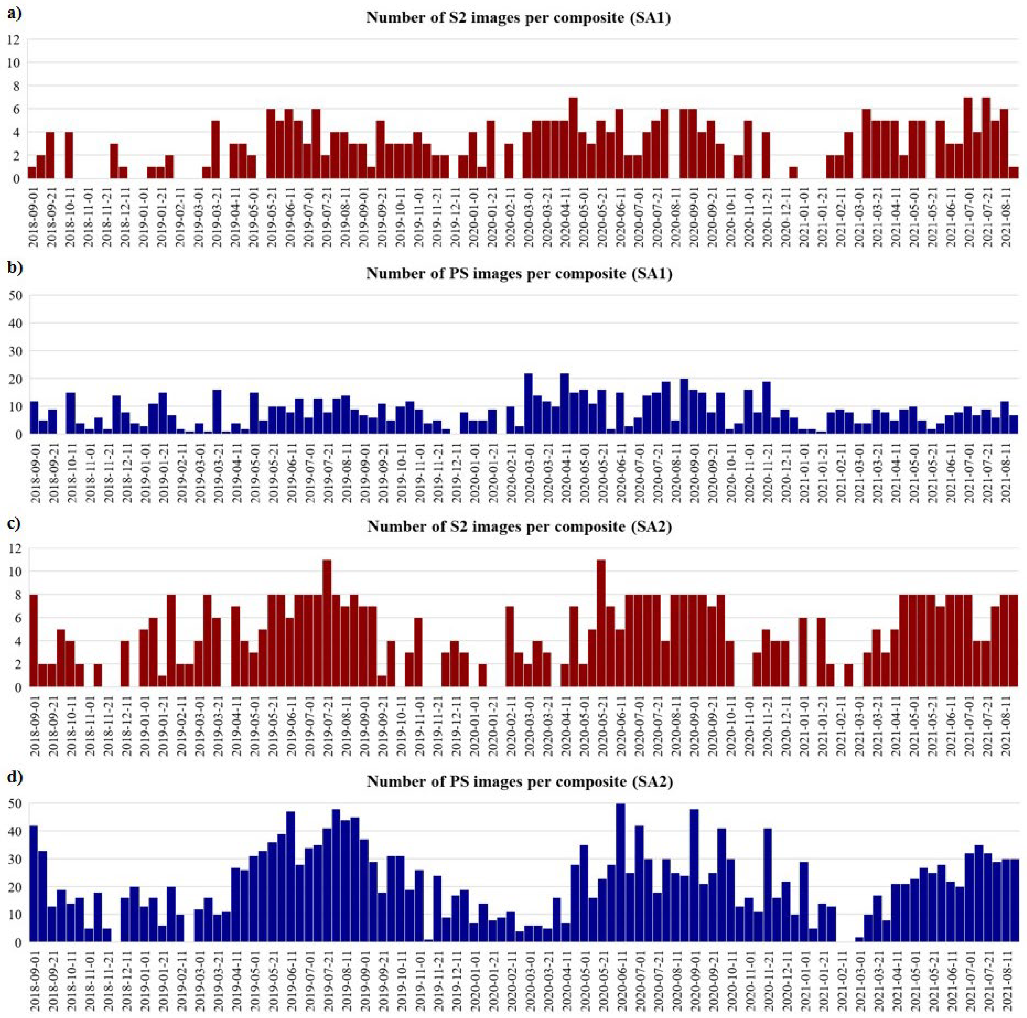
For data fusion, we adapted the method developed by Sadeh et al. [18], which processed S2 and PS images to obtain a consistent time series of fused images with temporal resolution of 10 days and 3 m of spatial resolution. Thus, we clipped both image sets considering the boundaries of each study area. We computed 10-day median compositions for the entire S2 and PS time series separately, making them consistent in interval and length. This procedure resulted in 36 images for each agricultural year from the corresponding data. The number of images used to calculate each composite in the study areas varied depending on image availability and the temporal resolution of the S2 and PS data (Figure 3). The median composition has already proven its applicability to form multi-sensor compositions in consistent time series [35]. In addition, the 10-day interval better corresponds to the dynamics in highly managed land uses. In the next step, the spectral bands of both data sources were separated, and then we applied linear interpolation to fill in the gaps in the SITS caused by cloud cover.

Figure 3.
Image frequency over the time series to generate the 10-day median composites, considering S2 data in SA1 (a) and SA2 (c), and PS data in SA1 (b) and SA2 (d).
Subsequently, the data fusion steps described by Sadeh et al. [18] (for additional information, see Section 2.3 on that study) were performed. These steps involved initially resampling the S2 data pixels using cubic interpolation from 10 m to 3 m. Later, we separated the RGB-NIR bands from S2 (resampled) and PS to fuse the data by averaging the pixel values from each pair of bands. We represented all steps of the fusion process in a workflow, Figure 4.
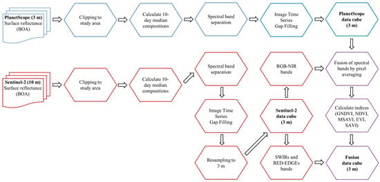
Figure 4.
Workflow for obtaining the three data cubes formed by S2, PS, and DF (in bold).
The described data fusion process resulted in three data cubes from different data sources (Table 1), built from S2, PS, and DF data, with a temporal resolution of 10 days and a spatial resolution of 3 m. In addition, we calculated five spectral indices related to the state and vigor of the crops and soil properties, incorporating them into each data cube. The spectral indices were: Enhanced Vegetation Index (EVI) [36], Normalized Difference Vegetation Index (NDVI) [37], Green Normalized Difference Vegetation Index (GNDVI) [38], Modified Soil-Adjusted Vegetation Index (MSAVI) [39], and Soil-Adjusted Vegetation Index (SAVI) [40]. The time series of all spectral bands and indices were used for developing the classification models. Specifically, the PS data cube consisted of nine layers, while the S2 and DF data cubes each contained 14 layers, as detailed in Table 1.

Table 1.
Spectral bands and spectral indices contained in the data cubes.
2.5. Dataset Partition
Although this research was based on a pixel-based approach, we used a multitemporal image segmentation method for splitting the training and testing data. This process was performed to ensure that the samples were spatially disjoint and that samples inserted in the same polygon were not simultaneously in the training and test set. We applied the Simple Non-Iterative Clustering (SNIC) algorithm [41], a variation of the superpixel algorithm available on the Google Earth Engine platform [42]. We provided the time series of fused NDVI images for each agricultural year (36 images) in both study areas as input to the algorithm. The generated polygons considered the spectro-temporal dynamics of areas with agricultural intensification [43]. We adjusted the following parameters: compactness (0.5), connectivity (4), neighborhoodSize (256) and seed grid equal to 50 and 140 for SA1 and SA2, respectively. The parameters were fine-tuned based on visual assessment aiming at the most suitable output.
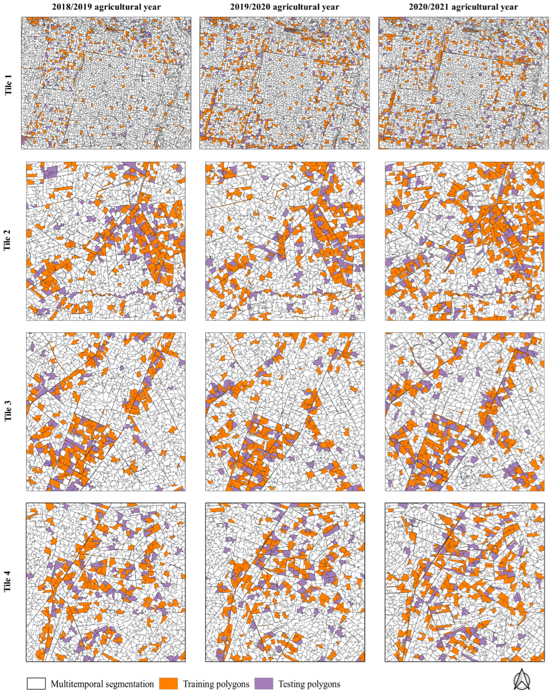
Using the resulting multitemporal segmentation polygons (Figure 5), we divided the labeled samples into 70% for training and 30% for testing through a random and stratified process, considering each agricultural year. Thus, we overlapped the field data with the polygons to generate the entire dataset (Table 2).
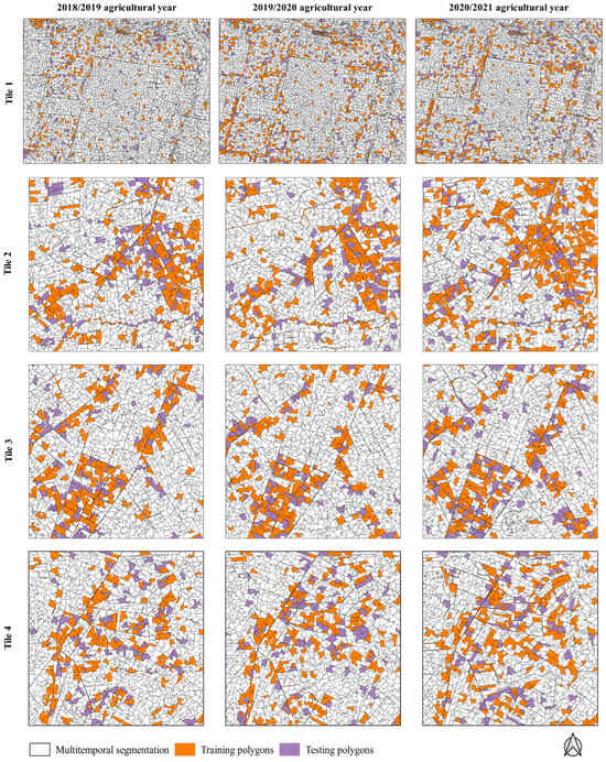
Figure 5.
Multitemporal segmentations generated for SA1 (Tile 1) and SA2 (Tiles 2, 3 and 4) by agricultural year and its polygons, which were used for splitting the training (70%) and test (30%) datasets.
Table 2.
The distribution of samples, partitioned into training and testing sets from multitemporal segmentation polygons, considering each class and agricultural year in both study areas, where CPA: Cultivated Pasture, DCP: Double Crop, EUC: Eucalyptus, FOR: Forest, NVW: Natural vegetation and wet areas, OTH: Others, PCS: Pasture consortium, PRC: Perennial crops, SPC: Semi-perennial crops, WAT: Water.
All classifications, result evaluations, and prediction workflows were performed in “sits: Satellite Image Time Series Analysis on EO Data Cubes”, an R package [34]. To handle the time series data in this package, we used the ground reference data points to extract the corresponding values of each composition and its spectral bands and store them within a tibble data structure, as described in Simoes et al. [34]. The tibble time series contained spatial and temporal information, as well as the labels assigned to the samples. For each data cube representing the three scenarios (S2, PS, and DF), we created their respective training and testing tibbles. These structured data was used to compare scenarios and evaluate the performance of the classification algorithms.
2.6. Machine and Deep Learning Algorithms for ICLS Classification
We tested four algorithms for ICLS classification using the three data cubes. RF [44] is used as a baseline classifier in our study. RF is an ensemble method based on decision trees, which uses a randomly selected subset of training samples and variables in building each tree. Thus, to build the trees, the two most important parameters are needed, namely the number of trees (ntree) and the number of variables used to split the internal nodes of the decision trees (mtry). When choosing these parameters, we followed the suggestion of previous works [45], defining ntree as equal to 1000 and mtry as equal to the square root of the total number of features.
We assessed the performance of the TempCNN [22] and the ResNet [23] due to the ability of these networks to account for the temporal ordering of samples in SITS [34]. In addition, the convolution layers play an important role in feature extraction by applying one-dimensional filters to detect temporal patterns in time series classification [46]. Thus, we followed Pelletier et al. [22] who proposed the TempCNN architecture (Figure 6a) with three consecutive 1D convolutional layers (64 units), followed by a dense layer (256 units) and a softmax layer. The ResNet architecture (Figure 6b) is deeper, being composed of nine convolutional layers equally distributed in 3 blocks, the first with 64 units and the others with 128. This structure is followed by a global pooling layer that averages the time series along the temporal dimension and, finally, a softmax layer. The advantage of ResNet is the residual shortcut connection between consecutive convolutional layers. Wang et al. [23] proposed combining the input layer of each block with its output layer through a linear shortcut, thus allowing the flow of the gradient directly through these connections and avoiding the so-called vanishing gradient problem.
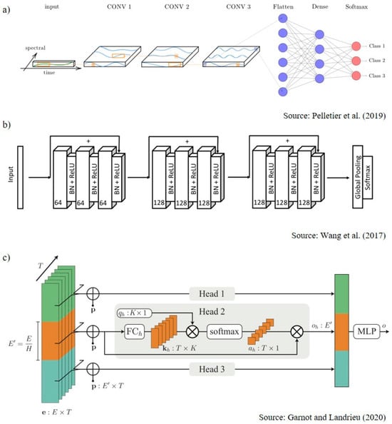
Figure 6.
The architectures of the deep learning neural networks used in our research: (a) TempCNN [22], (b) ResNet [23], and (c) L-TAE [24].
Lastly, we used the state-of-the-art L-TAE [24]. This architecture (Figure 6c) employs self-attention and positional encoding mechanisms. The self-attention mechanism can identify relevant observations and learn contextual information in a time series for classification [47]. Positional coding ensures that the sequential ordering of the elements of a time series is maintained throughout the learning of the neural network [47]. Another advantage of this architecture comes from the concept of multi-heads, which allows different sets of parameters to be trained in parallel on the network independently, so-called attention heads. In this way, each head becomes specialized in detecting different patterns, and its output is then concatenated with the other heads. Thus, for the application of L-TAE, we tested the fusion of data cubes coming from S2 and PS within the temporal encoder from the concatenation of all bands, following the early fusion strategy presented by Ofori-Ampofo et al. [20] and Garnot et al. [21]. Ofori-Ampofo et al. [20] stated that this type of strategy is recommended when the target classes are underrepresented as it is the case with ICLS. In this case, we tested the early fusion strategy in L-TAE architecture as a second method to fuse data and classify ICLS fields. This step aimed to verify which fusion approach would be the most suitable for ICLS mapping.
Deep learning networks employ stochastic gradient descent methods to achieve optimal performance. These methods accelerate predictions and convergence compared to exhaustive testing of all parameter combinations. For this purpose, some optimization algorithms select hyperparameters randomly, resulting in the best combination of them [48]. The main hyperparameters include the learning rate, which controls the numerical step of the gradient descent function; epsilon (ε), which controls numerical stability; and weight decay, which controls overfitting. In our research, the three deep learning algorithms were trained with the AdamW optimizer [49], using standard parameter values obtained from the sits_tuning function in the sits package [34]. Thus, the coefficients used for computing running averages of the gradient and its square were β1 = 0.9 and β2 = 0.999, ϵ = 1 × 10⁻⁸, the weight decay was equal to 1 × 10⁻⁶, the learning rate was equal to 0.001, and the validation set was corresponding to 20% of the training set. We set a batch size of 64 (number of samples per gradient update) and the maximum number of epochs to 150 with a patience of 20.
2.7. ICLS Classification and Mapping Performance Evaluation
We assessed the performance of RF and the deep learning architectures (TempCNN, ResNet, and L-TAE) across the three input data source scenarios. From the dataset separated for training (70%), we evaluated the performance of scenarios and algorithms using the k-fold cross-validation method (5 folds), repeated five times. Thus, we used the average accuracies in a t-test (assuming equal variances) to compare the performance of the models obtained from the three scenarios (S2, PS, and DF). Subsequently, we used the testing set (30%) to compare the performance of the algorithms and choose the best model considering an independent data set.
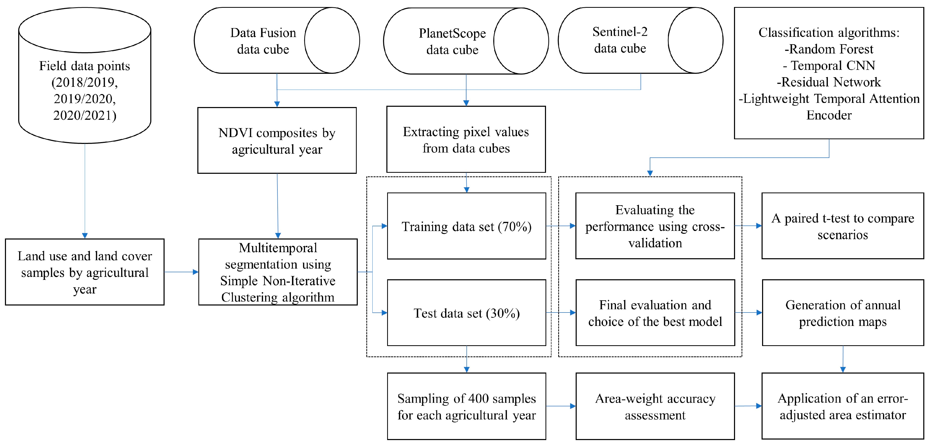
To generate the annual prediction maps for both study areas, we classified the data cubes using the best model through parallel processing to speed up the performance, as described by Simoes et al. [34]. As a result of the classification, an output data cube was generated containing probability layers, one for each output class, which brings information about the probability of each pixel belonging to the related class. In this case, we assigned the pixel to the highest probability class. Furthermore, we applied a smoothing method based on Bayesian probability that uses information from the pixel neighborhood to decrease the uncertainty about its label and reduce salt-and-pepper effects [34]. In this case, we defined the main parameters for performing Bayesian smoothing in the sits package: window size (9), neighborhood fraction (0.5) and smoothness (20). Figure 7 illustrates the steps of the method proposed to map ICLS.
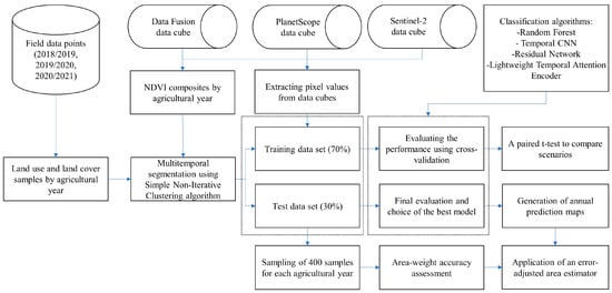
Figure 7.
Workflow with the main steps of the proposed method, considering the three data cubes from different sources and machine and deep learning algorithms for mapping ICLS.
To measure the accuracy of the resulting prediction maps, we applied the area-weighted accuracy assessment technique, following the best practices proposed by Olofsson et al. [50] and the practical guide from FAO [51]. For this purpose, we used the polygons extracted by the multitemporal segmentation for testing (30%) and sampled about 400 samples for each agricultural year through a random and stratified process. The size of the sample set considers the proportion of mapped area for each class, providing an expected standard error of global precision of 0.05 [50]. In addition, we applied an error-adjusted estimator of area along with confidence intervals to eliminate the bias attributable to the classification of the final maps, as described by Olofsson et al. [52].
Thus, for each annual classification map, we obtained confusion matrices to calculate the following performance metrics: Overall Accuracy (OA), User (UA) and Producer accuracy (PA), and F1-Score for the ICLS class.
3. Results
3.1. ICLS Spectro-Temporal Patterns Computation Using Different Data Sources
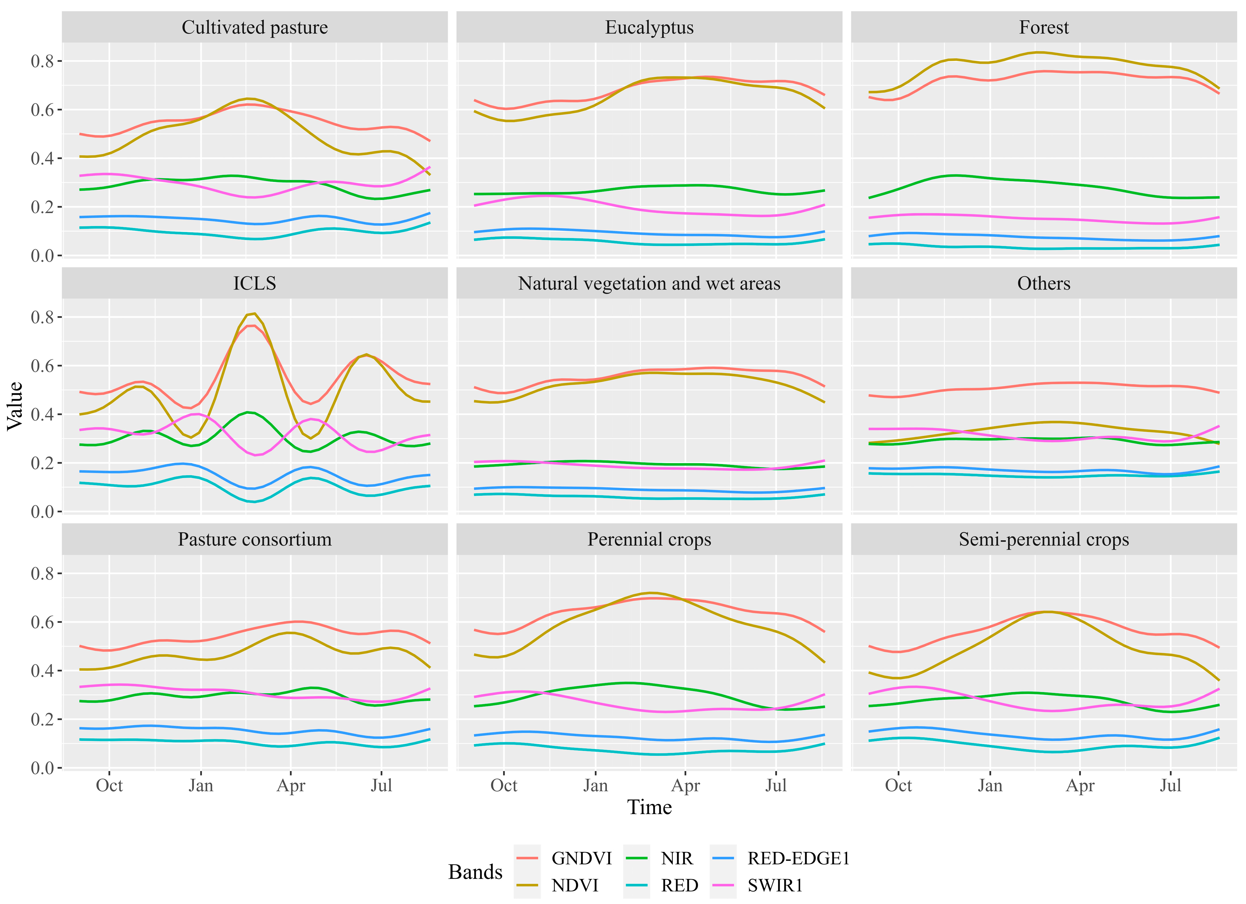
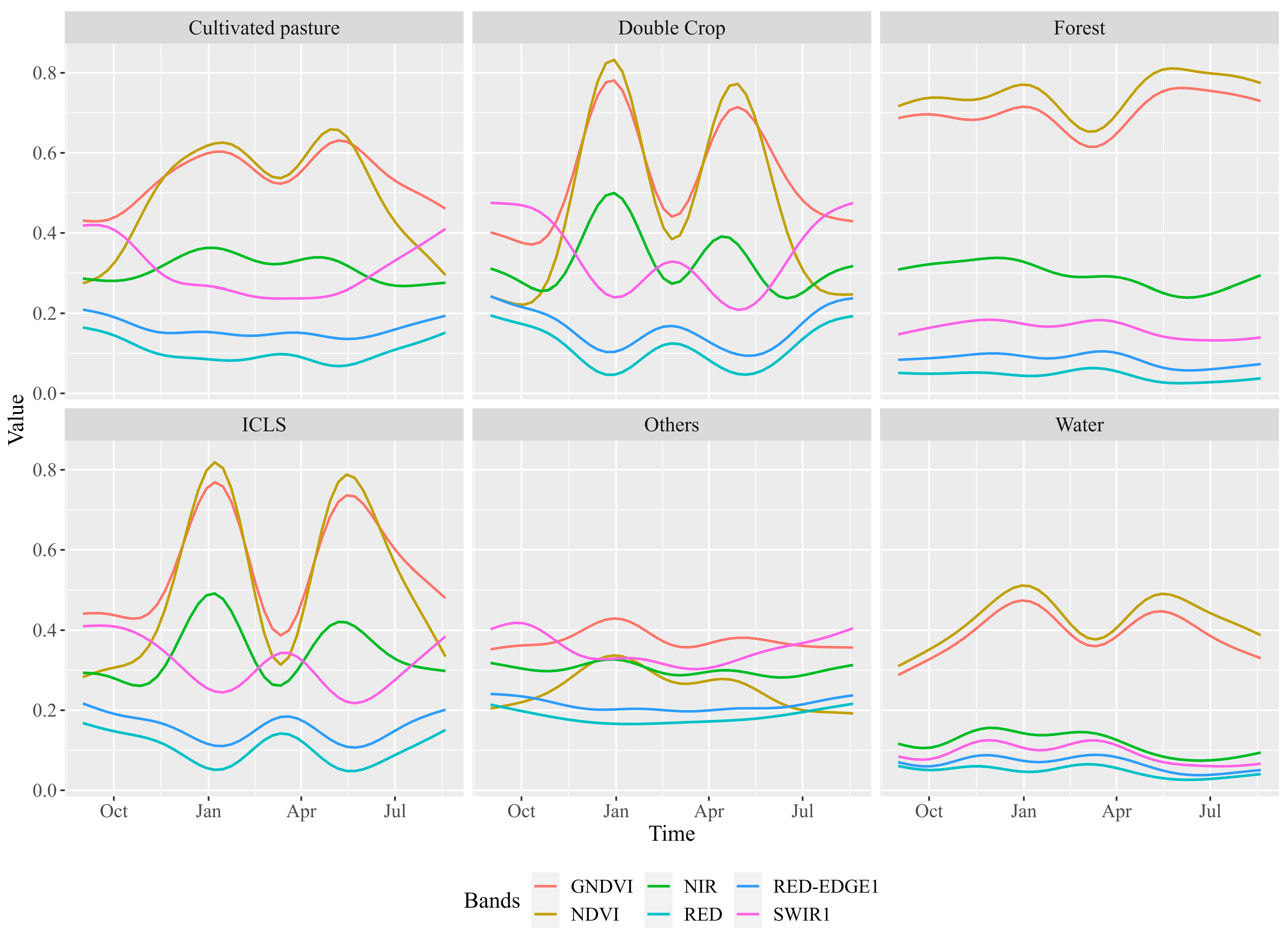
Figure 8 and Figure 9 show the spectro-temporal patterns for each target class present in SA1 and SA2, respectively. The patterns were produced using a generalized additive model to estimate a statistical approximation to an idealized pattern per class [53]. We highlight the similarity of the patterns observed among Cultivated pasture, Perennial crops, and Semi-perennial crops in SA1, as well as the similar patterns between Double crop and ICLS in SA2.
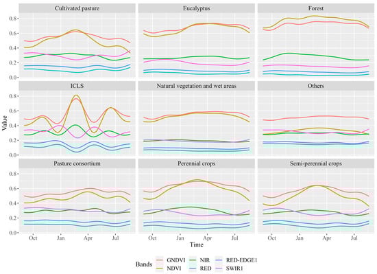
Figure 8.
Estimated temporal patterns of the GNDVI, NDVI, NIR, Red, Red-edge 1, and SWIR 1 bands extracted from the data fusion cube for the LULC classes in SA1.
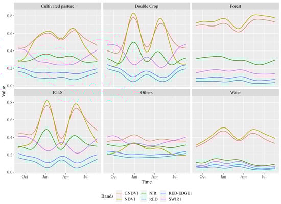
Figure 9.
Estimated temporal patterns of the GNDVI, NDVI, NIR, Red, Red-edge 1, and SWIR 1 bands extracted from the data fusion cube for the LULC classes in SA2.
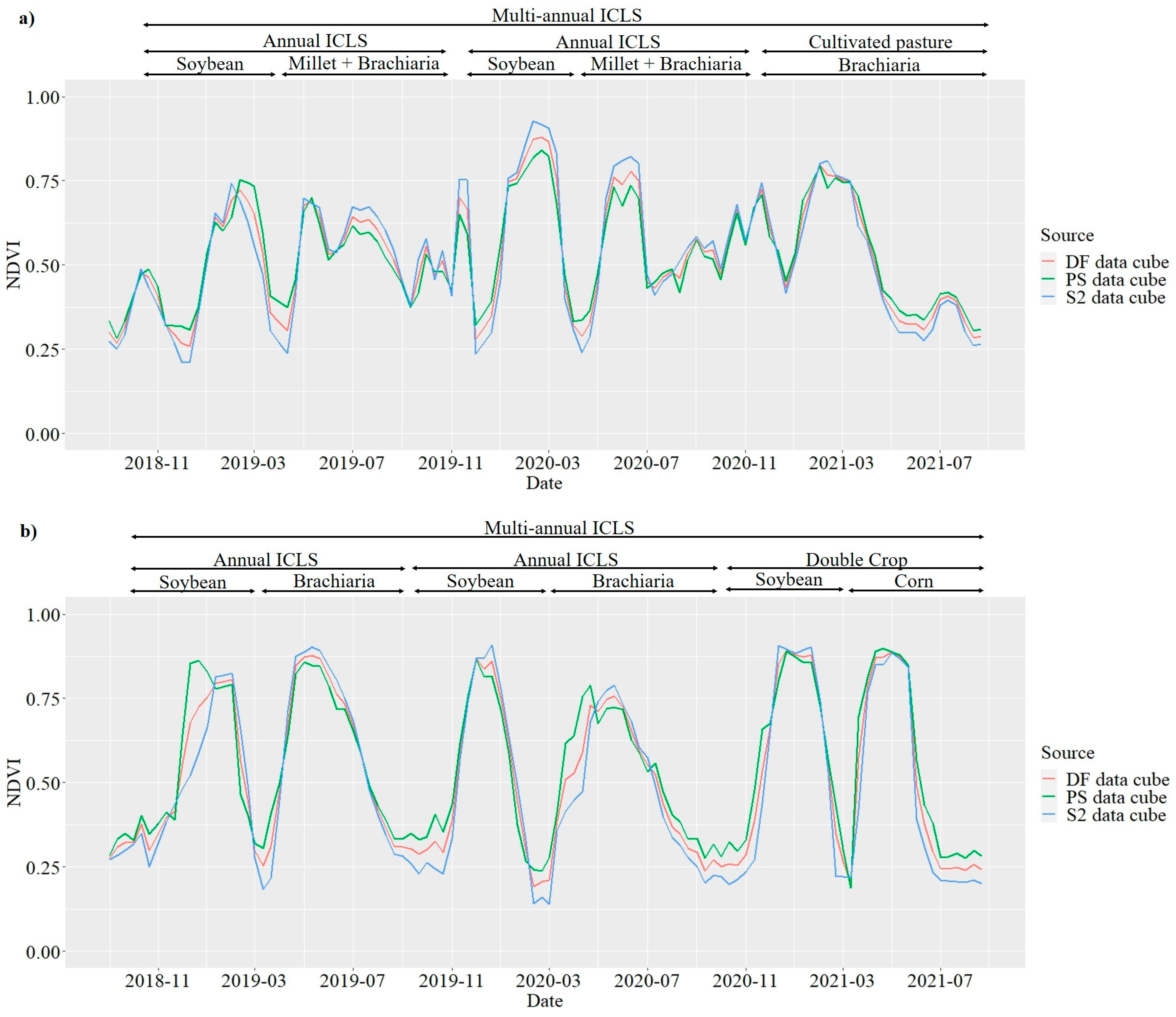
Figure 10 represents the three-year average spectro-temporal NDVI profile obtained from the data cubes in two fields with ICLS for SA1 (Figure 10a) and SA2 (Figure 10b), with field sizes of 19 and 63 hectares, respectively. Based on the NDVI temporal patterns, we observed that the different data sources have similar patterns along the time series and represent well the land use dynamics in fields of ICLS. However, in general, vegetation indices based on S2 data were more sensitive to high and low values, which are related to crop phenological stages and green biomass. PS temporal patterns showed more variation and less sensitivity to high and low NDVI values than S2 data. On the other hand, the DF data showed average values between the two sources, as expected. We also identified distinct patterns indicative of specific management strategies in ICLS, where a combination of crop and pasture cultivation occurs in succession or rotation. Rotation practices were represented by the management of soybeans alternated with pastures. In contrast, succession was represented by managing two agricultural years as annual ICLS followed by a year of Cultivated pasture (Figure 10a) or Double crop (Figure 10b).
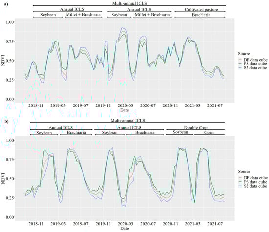
Figure 10.
Average NDVI temporal patterns of ICLS present in SA1 (a) and SA2 (b), demonstrating annual and multi-annual ICLS management strategies.
By defining an annual ICLS classification method, we use information from the first and second crop seasons within an agricultural year, when the crops are followed by simple pastures (Figure 10b) or mixed pastures (Figure 10a). On the other hand, when using information from all years, the multi-annual analysis considers the sequence of crop types over the years. The importance of the multi-year analysis can be demonstrated when considering a scenario where the analysis is restricted to one agricultural year, specifically the most recent year (2020/2021). In this scenario, the land use in the two fields featuring ICLS would probably be classified as Cultivated pasture (as shown in Figure 10a) and Double crop (as shown in Figure 10b).
3.2. Assessment of the Classification Results
The results obtained from the five cross-validations showed a slight superiority, no more than 0.5% of OA, when using DF (92.1%—SA1, 96.1%—SA2) compared to other scenarios that used S2 (91.7%—SA1, 95.8%—SA2) and PS (91.8%—SA1, 95.9%—SA2), considering both study areas. However, the t-test results indicate that there are no significant differences (p-value > 0.05) between the scenarios coming from the different data cubes for both areas.
When the classification results were assessed based on the testing set, the performance of the classifiers was maintained (Table 3), which demonstrated the generalization capacity of the previously trained models. In SA1, TempCNN (OA = 90.0%) was again the best classifier, while in SA2, TempCNN (OA = 95.6%) and RF (OA = 95.5%) also showed the best OA results, with DF being the best scenario for LULC classification in both study areas. PA and UA for the ICLS class were equal to or better than 94.4% and 89.7% in SA1 and 78.5% and 82.2% in SA2, respectively. ResNet had the worst performance for both study areas (79.7% and 94.4%, respectively) using non-fused data, since this algorithm is more difficult to parameterize. The highest F1-score values for the ICLS class were obtained by TempCNN (100.0%) and L-TAE (100.0%) in SA1 and by RF in SA2 (89.3%).
Table 3.
Classification results of the test data, in percentages, obtained by the four classifiers using data cubes from three different scenarios in classifying the study areas.
The agreement results of the prediction achieved by the best classifier (TempCNN) show the confusion between classes in both areas (Figure 11). For instance, for the ICLS, the confusion occurred only with Cultivated pasture (2.8%) in SA1 (Figure 11a), even with a low proportion, while in SA2 (Figure 11b), the most significant confusion of ICLS was with Double crop (6.2%), followed by Cultivated pasture (1.7%). The F1-score results for ICLS (Table 3) indicate greater difficulty in identifying ICLS in SA2 (86.6%) than SA1 (98.6%). The highest misclassification rate was found between Pasture consortium (37.0%) and Semi-perennial crops (23.0%) in SA1 (Figure 11a) to Cultivated pasture due to their inherent similarity regarding spectral characteristics and management practices.
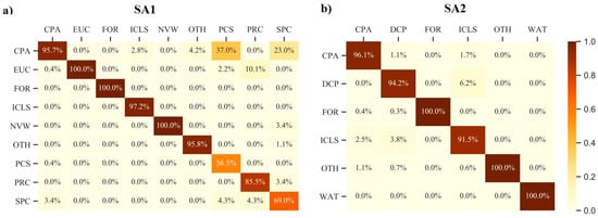
Figure 11.
Agreement percentage results between the values predicted by the TempCNN model and the reference values, considering SA1 (a) and SA2 (b), where CPA: Cultivated Pasture, DCP: Double Crop, EUC: Eucalyptus, FOR: Forest, NVW: Natural vegetation and wet areas, OTH: Others, PCS: Pasture consortium, PRC: Perennial crops, SPC: Semi-perennial crops, WAT: Water.
3.3. Spatial Representation of the Classification Results
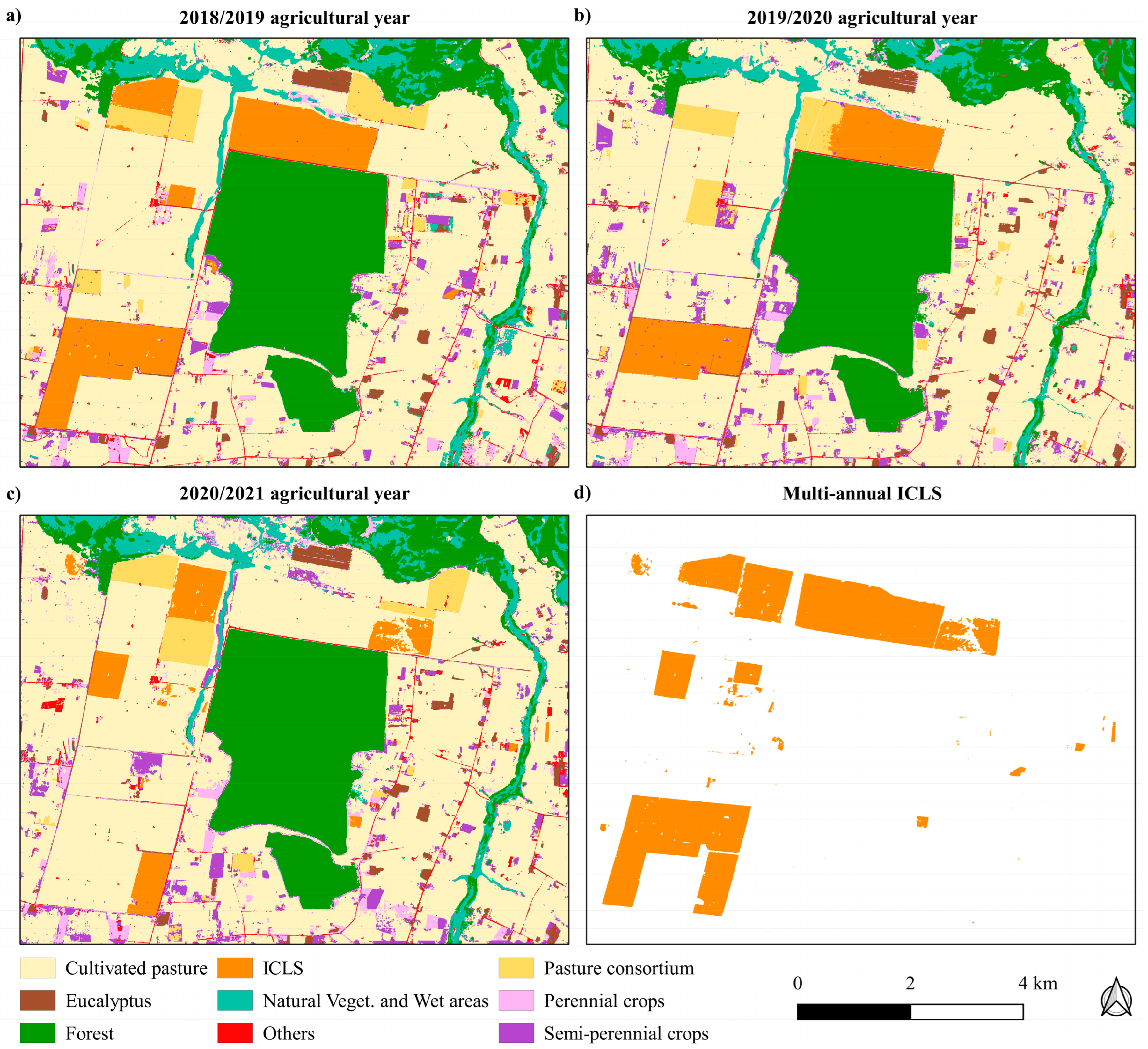
To generate the annual LULC maps for SA1 (Figure 12) and SA2 (Figure 13), TempCNN models were used to classify the DF data cubes by agricultural year, based on their superior prediction performance on the testing set and their enhanced generalization capacity. In both study areas, spatio-temporal changes in the ICLS areas were the result of their management practices. To address multi-annual ICLS mapping, we overlapped the information from the annual prediction maps to obtain the final classification for ICLS in both study areas.
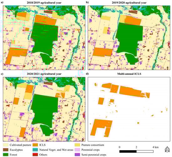
Figure 12.
Prediction maps for SA1 by agricultural year (a–c) and the final map (d) of fields with ICLS considering the multi-annual approach.
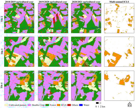
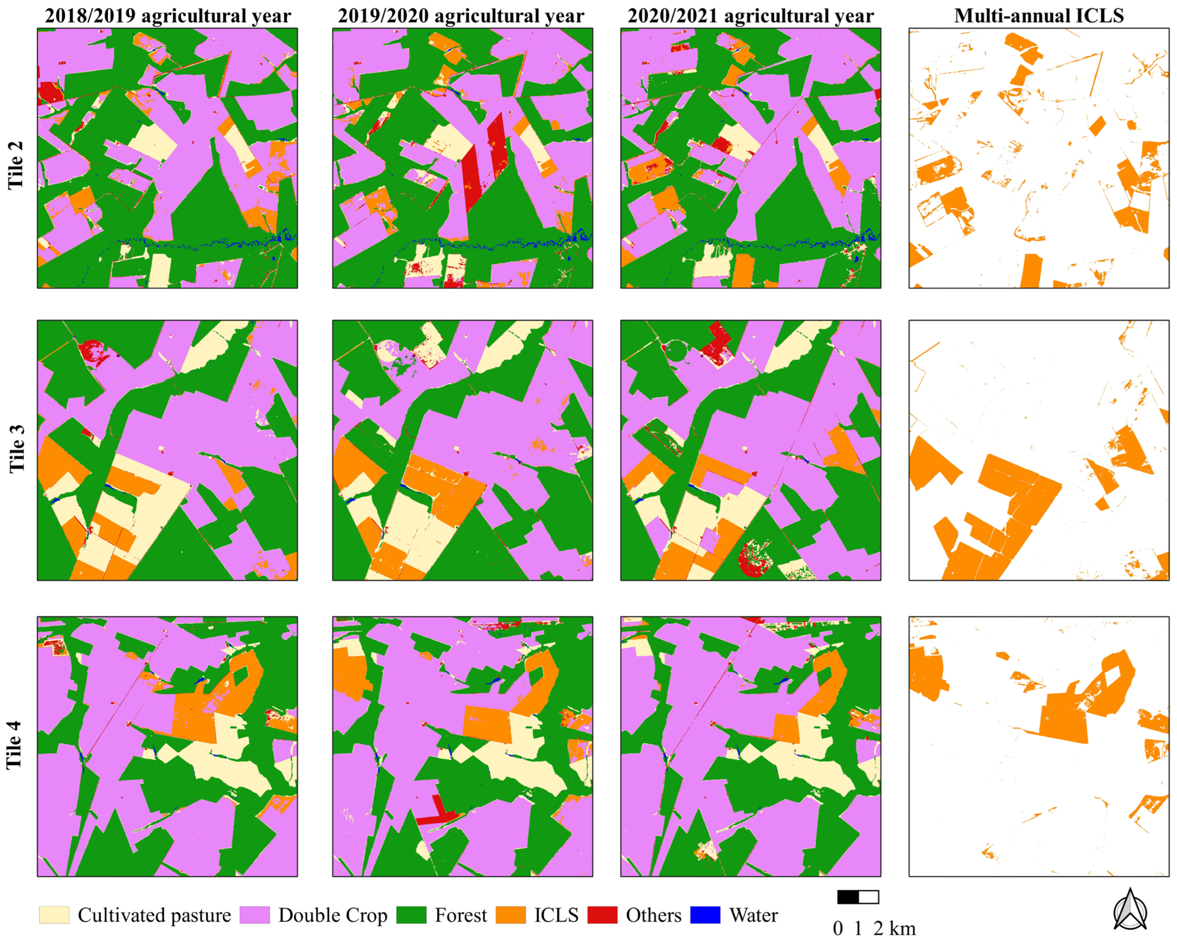
Figure 13.
Prediction maps for each tile in the SA2 by agricultural year and their final map of ICLS considering the multi-annual approach.
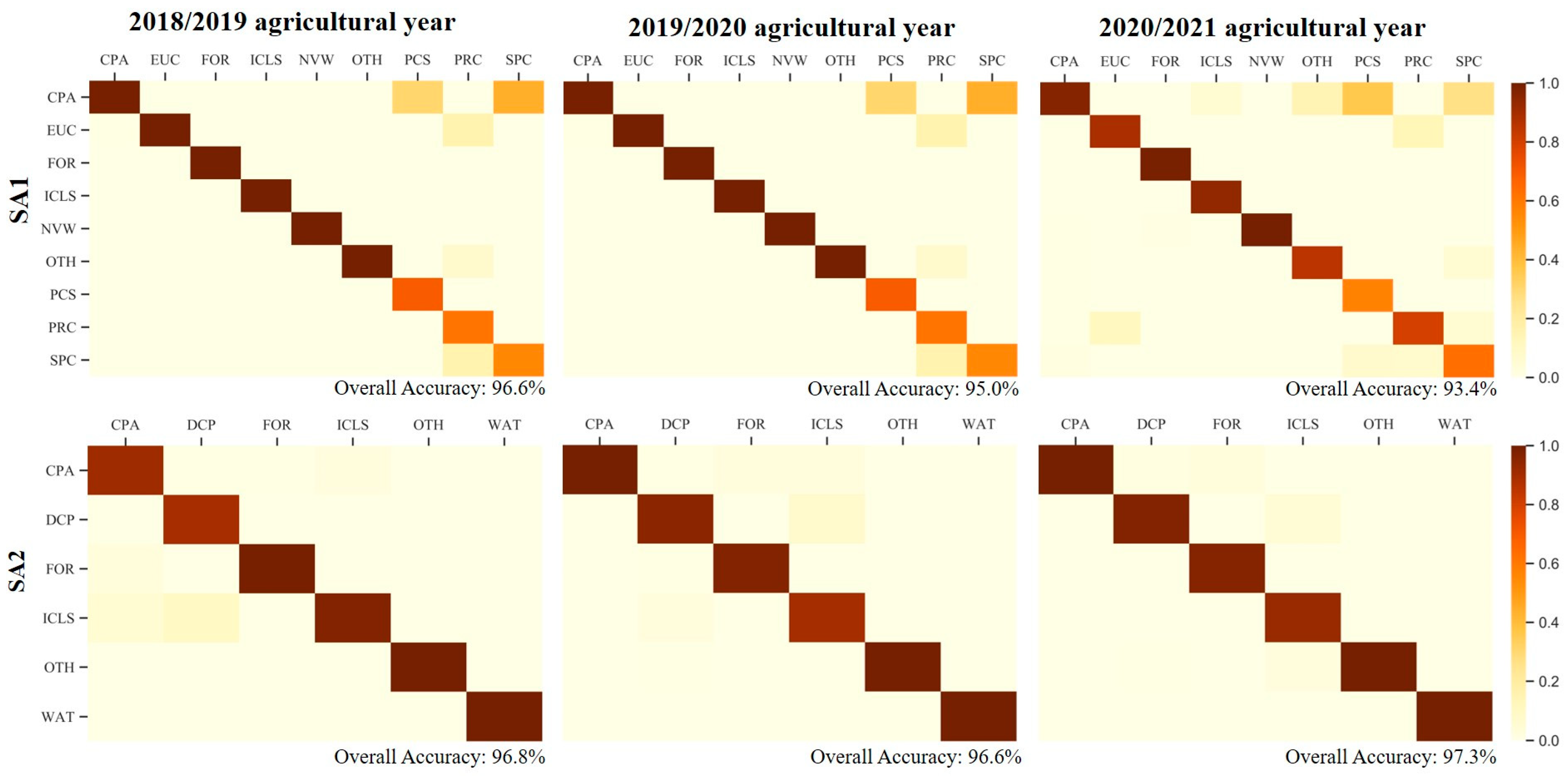
Table 4 presents the results of PA and UA by agricultural year for SA1 and SA2 considering the 95.0% confidence interval. For SA1, the classes Cultivated pasture, Natural vegetation and Wet areas, and ICLS reached the highest PA and UA values, all higher than 90.0%. In contrast, Semi-perennial crops, Pasture consortium, and Others had lower PA and UA values, which were close to or greater than 60.0% in SA1. These results can be explained by the fact that less frequent classes are more prone to errors than other classes prevalent in an unbalanced dataset. In terms of OA of the prediction maps obtained for SA1, all annual maps resulted in high OA values (Figure 14), with the agricultural year 2020/2021 having the lowest accuracy (93.4%) and the agricultural year 2018/2019 having the highest accuracy (96.6%).
Table 4.
The unbiased estimate of UA and PA for each class by agricultural year in SA1 and SA2, considering 95.0% confidence interval, where CPA: Cultivated pasture, DCP: Double crop, EUC: Eucalyptus, FOR: Forest, NVW: Natural vegetation and wet areas, OTH: Others, PCS: Pasture consortium, PRC: Perennial crops, SPC: Semi-perennial crops, WAT: Water.
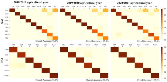
Figure 14.
Error matrices obtained in the evaluation of prediction maps using the sample set that considers the proportion of mapped areas for each class, considering SA1 and SA2, where CPA: Cultivated pasture, DCP: Double crop, EUC: Eucalyptus, FOR: Forest, NVW: Natural vegetation and wet areas, OTH: Others, PCS: Pasture consortium, PRC: Perennial crops, SPC: Semi-perennial crops, WAT: Water.
For SA2, Water, Forest, and Double crop classes had the highest PA and UA values, all greater than 97.0%. However, the Cultivated pasture, Others, and ICLS classes were predicted less accurately, showing PA and UA values close to or greater than 70.0% (Figure 14). We highlight the confusion between the target class of ICLS and Double crop due to the spectro-temporal similarity between these classes. In the 2018/2019 agricultural year, there were more commission errors for the ICLS class. When considering the two last agricultural years, the UA values for ICLS were above 90.0%. The OA results of the SA2 prediction maps were superior to those obtained in SA1, with the highest OA value in the 2020/2021 agricultural year (97.3%) and the lowest OA value in the 2018/2019 agricultural year (96.8%).
We adjusted the areas estimated by the best-performing classifiers using an area error-adjusted estimator, described by Olofsson et al. [52] (Figure 14).
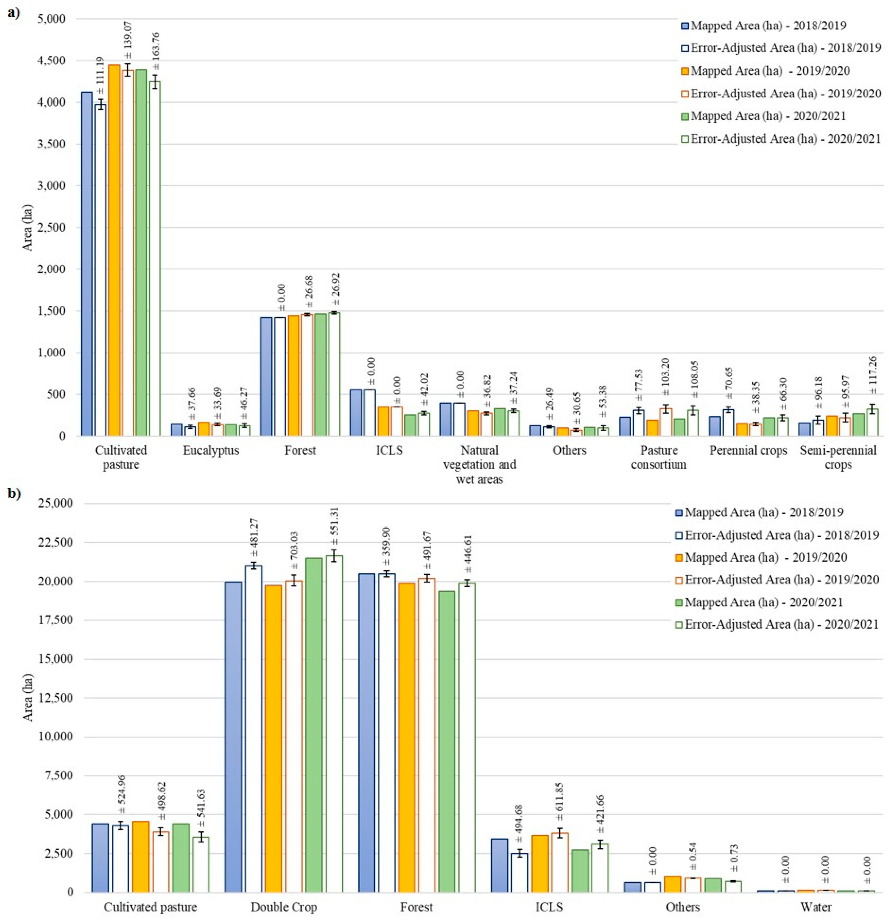
For SA1, these adjustments for the Forest and ICLS classes were almost null over the mapped area (Figure 15a), indicating good classification results. However, Cultivated pasture class returned a greater adjustment in area size, while the Pasture consortium, Perennial crops, and Semi-perennial crops classes were proportionally more adjusted concerning their total area.
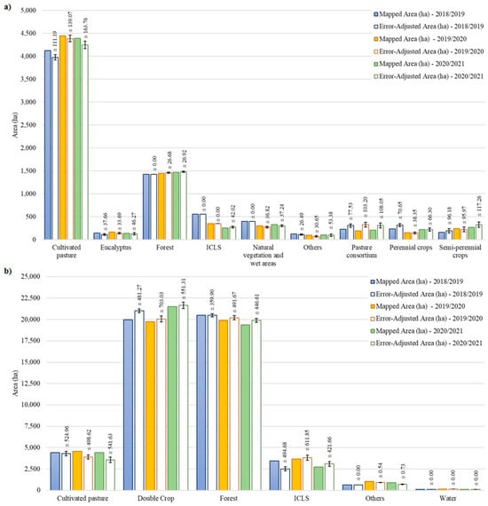
Figure 15.
Mapped area and adjusted area using the information from the error matrix (at 95.0% confidence interval) of each class for the three agricultural years, considering SA1 (a) and SA2 (b).
For SA2, there were no significant differences between the error-adjusted areas (Figure 15b) and the mapped area for the Other and Water classes because they have different spectro-temporal patterns compared to other non-vegetated classes. The total area of annual ICLS over the evaluated agricultural years is lower than the Cultivated pasture and Double Crop classes.
4. Discussion
4.1. Data Cubes and Their Spectro-Temporal Patterns for ICLS
The three data cubes (S2, PS, and DF) produced in this research have shown high capability to capture the phenological development of crops and pastures in fields managed as ICLS. Similar to the findings of Sadeh et al. [18], our spectro-temporal profiles based on PS data (Figure 10) had more signal variations than those generated by S2 or DF data. This phenomenon has already been reported and may be related to cross-sensor variations in surface reflectance values of images from the CubeSat PlanetScope constellations [19]. In this context, combining data from different sources provided a consistent time series of fused data. These results align with those obtained by Griffiths et al. [35], who reported the importance of the applicability of multi-sensor image composition to monitor dynamic targets on the Earth’s surface.
4.2. ICLS Classification Results Using Different Data Cubes and Deep Learning Algorithms
Although there were no significant statistical differences between the three scenarios, the classification results using DF data cube were slightly better in all experiments compared to other data cubes (Table 3). Furthermore, the results derived from the fusion method employing L-TAE algorithm indicate that early fusion of data cubes within the temporal encoder offers advantages in terms of classification performance and processing time. Further research should explore decision-level fusion approaches [20]. The classification results obtained using only the S2 data cube showed that this dataset was suitable for identifying ICLS and other dynamic land uses in our study areas, highlighting the potential of S2 data cubes for large-scale mapping approaches. On the other hand, a greater gain in using DF and PS data cubes could occur in regions where agricultural fields are smaller. It is worth mentioning that pre-processing steps required to build the data cubes, such as computing the 10-day median compositions and filling in gaps, were essential to reduce the noise caused by clouds, especially in rainy months (November to March in our study areas). However, in rainy years or regions with very high cloud coverage, we expect a decrease in the performance of the classification models.
Regarding the performance of the evaluated algorithms (presented in Table 3), the studies of Pelletier et al. [22] and Zhong et al. [54] also revealed that 1D-CNN models obtained the highest accuracy for crop classification. This high performance may be attributed to their ability to take into account the temporal information and capture seasonal patterns of SITS. The performance achieved by RF in SA2 (95.4%) was close to the best-performing model based on deep learning (TempCNN—95.5%). This result may be related to the greater homogeneity and larger size of agricultural fields in SA2 than in SA1, which is further evident by the representation of SA2 in fewer classes. The slightly lower performance of the ResNet algorithm (88.5%—SA1, 94.6%—SA2) may potentially be improved through further experimentation with different filter sizes. Similar to Ofori-Ampofo et al. [20], who obtained an OA of 92.2% in crop classification, our study also obtained high accuracy when applying L-TAE to classify target classes in the two areas (88.4%—SA1, 94.7%—SA2), demonstrating the importance of data fusion by this architecture. The success of deep learning neural networks in achieving high accuracies may be attributed to the quality of the training samples [55] and their geographic distribution [56]. In our study, we ensured high-quality training samples and an optimal geographic distribution through the implemented multitemporal segmentation process.
4.3. ICLS Mapping in the Study Areas
The highest OA for SA2 may be related to a more homogeneous landscape compared to SA1, mainly represented by a lower number of land use classes and a larger area. In contrast, we had higher F1-Score results for ICLS in SA1 (0.99) than SA2 (0.87), mainly due to the misclassification between ICLS and Double crop in SA2. These two classes have similar spectro-temporal patterns (Figure 9) due to the implemented agricultural management practices during the agricultural year. Double crop and ICLS encompass soybean that is primarily cultivated as a summer crop subsequently followed by either another crop (e.g., corn, millet, or crotalaria) in Double crop or pasture in ICLS. Previous studies have also emphasized the challenge of discriminating Double crop and ICLS [13,14,15]. Our results showed an accuracy improvement compared to previous works focused on mapping ICLS that used data from MODIS sensor [13,14] and very close accuracy obtained in the study of Toro et al. [15], which used S1 and S2 SITS. The quality of the prediction maps obtained from the fused time series was high for SA1, where the field size is smaller. This accuracy gain is explained by using high spatial resolution PS data, which allows classifying ICLS in small fields compared to previous works that used coarser resolution images in the same region [15]. The imbalanced sample distribution across the target classes increased the accuracy of the major classes at the expense of the accuracy of the minor classes. To address this challenge, balancing methods such as those presented in Waldner et al. [57] should be considered.
Our study revealed a reduction in the total area occupied by ICLS over the agricultural years in SA1 (Figure 15a). The multi-annual dynamics of these areas necessarily can be caused by the price fluctuations in the market and by the farmers’ decision-making on the management of their lands [30].
While our research focused on only two study areas, it is important to highlight that they are located in a widespread ICLS region in Brazil. In light of the necessity for more robust mapping techniques to support sustainable and dynamic agricultural production systems, the developed method could be tested in other regions with ICLS. Nevertheless, the trained deep learning models may have limited transferability to areas with different agricultural management practices and climatic conditions. In this context, including samples encompassing site-specific ICLS characteristics could increase the transferability of pre-trained models.
To summarize, this research contributes to generating total area estimates and identifying the spatial distribution of ICLS by proposing an end-to-end workflow using state-of-the-art techniques. This workflow is useful for sectors interested in monitoring this type of agricultural production system.
5. Conclusions
Our study proposed a method that combines SITS data cubes and deep learning to effectively map annual ICLS under different agricultural management practices in two diverse landscapes in Brazil.
This study showed that the S2 data cubes were suitable for classifying ICLS successfully in the investigated study areas, whereas high spatial resolution PS data improved only slightly the classification accuracy results obtained by the PS and DF data cubes. Among the classifiers, wTempCNN outperformed the other investigated classifiers, indicating its superior ability to learn the spectro-temporal patterns associated with the target class. RF performed similarly to TempCNN in the SA2, where the landscape is more homogeneous and composed of larger agricultural fields than the SA1. Further, the L-TAE demonstrated the possibility to fuse data from different sources within temporal encoders, eliminating the need to generate synthetic images. Finally, ResNet performed was the least effective among the tested classifiers. The ICLS mapping results presented in this study open up the possibility of extending the analysis to broader regions within Brazil and other countries that adopt integrated systems. This expansion holds promise for fostering more sustainable agricultural production practices on a larger scale, thereby contributing to the advancement of environmentally responsible farming methodologies worldwide.
Author Contributions
Conceptualization, J.P.S.W., M.B., J.C.D.M.E. and G.K.D.A.F.; methodology, J.P.S.W., M.B., I.T.B., A.A.D.R., A.P.S.G.D.T., J.F.G.A., A.S., R.A.C.L., A.C.C., J.C.D.M.E. and G.K.D.A.F.; software, J.P.S.W. and J.C.D.M.E.; validation, J.P.S.W., M.B., J.C.D.M.E. and G.K.D.A.F.; formal analysis, J.P.S.W., M.B., J.C.D.M.E. and G.K.D.A.F.; investigation, J.P.S.W., M.B., J.C.D.M.E. and G.K.D.A.F.; resources, J.P.S.W., M.B., J.F.G.A., A.S., R.A.C.L., P.S.G.M., A.C.C., J.C.D.M.E. and G.K.D.A.F.; data curation, J.P.S.W. and A.A.D.R.; writing—original draft preparation, J.P.S.W. and M.B.; writing—review and editing, J.P.S.W., M.B., I.T.B., A.A.D.R., A.P.S.G.D.T., J.F.G.A., A.S., R.A.C.L., P.S.G.M., A.C.C., J.C.D.M.E. and G.K.D.A.F.; visualization, J.P.S.W., M.B., I.T.B. and G.K.D.A.F.; supervision, M.B., A.S., J.C.D.M.E. and G.K.D.A.F.; project administration, J.F.G.A., R.A.C.L., P.S.G.M. and G.K.D.A.F.; funding acquisition, J.F.G.A., P.S.G.M. and G.K.D.A.F. All authors have read and agreed to the published version of the manuscript.
Funding
This research was funded by the São Paulo Research Foundation (FAPESP), grant number: 2017/50205-9. The authors are thankful to the São Paulo Research Foundation (FAPESP) (Grants: 2018/24985-0 and 2021/15001-9), the National Council for Scientific and Technological Development (CNPq) (Grant: 305271/2020-2), and the Coordination for the Improvement of Higher Education Personnel (CAPES, Finance code 001).
Data Availability Statement
The raw data supporting the conclusions of this article will be made available by the authors on request.
Acknowledgments
The authors are grateful to FEAGRI/Unicamp and ITC/University of Twente for the infrastructure support provided for this project’s development.
Conflicts of Interest
The authors J.F.G.A., A.C.C. and J.C.D.M.E are employed by the Brazilian Agricultural Research Corporation (Embrapa). The remaining authors declare that the research was conducted in the absence of any commercial or financial relationships that could be construed as a potential conflict of interest.
References
- Cortner, O.; Garrett, R.D.; Valentim, J.F.; Ferreira, J.; Niles, M.T.; Reis, J.; Gil, J. Perceptions of Integrated Crop-Livestock Systems for Sustainable Intensification in the Brazilian Amazon. Land Use Policy 2019, 82, 841–853. [Google Scholar] [CrossRef]
- United Nations. Transforming Our World: The 2030 Agenda for Sustainable Development. Available online: https://www.un.org/sustainabledevelopment/news/communications-material/ (accessed on 7 February 2023).
- Sekaran, U.; Lai, L.; Ussiri, D.A.N.; Kumar, S.; Clay, S. Role of Integrated Crop-Livestock Systems in Improving Agriculture Production and Addressing Food Security—A Review. J. Agric. Food Res. 2021, 5, 100190. [Google Scholar] [CrossRef]
- Delandmeter, M.; de Faccio Carvalho, P.C.; Bremm, C.; dos Santos Cargnelutti, C.; Bindelle, J.; Dumont, B. Integrated Crop and Livestock Systems Increase Both Climate Change Adaptation and Mitigation Capacities. Sci. Total Environ. 2024, 912, 169061. [Google Scholar] [CrossRef] [PubMed]
- Monteiro, A.; Barreto-Mendes, L.; Fanchone, A.; Morgavi, D.P.; Pedreira, B.C.; Magalhães, C.A.S.; Abdalla, A.L.; Eugène, M. Crop-Livestock-Forestry Systems as a Strategy for Mitigating Greenhouse Gas Emissions and Enhancing the Sustainability of Forage-Based Livestock Systems in the Amazon Biome. Sci. Total Environ. 2024, 906, 167396. [Google Scholar] [CrossRef] [PubMed]
- Liebig, M.A.; Ryschawy, J.; Kronberg, S.L.; Archer, D.W.; Scholljegerdes, E.J.; Hendrickson, J.R.; Tanaka, D.L. Integrated Crop-Livestock System Effects on Soil N, P, and pH in a Semiarid Region. Geoderma 2017, 289, 178–184. [Google Scholar] [CrossRef]
- Bonaudo, T.; Bendahan, A.B.; Sabatier, R.; Ryschawy, J.; Bellon, S.; Leger, F.; Magda, D.; Tichit, M. Agroecological Principles for the Redesign of Integrated Crop–Livestock Systems. Eur. J. Agron. 2014, 57, 43–51. [Google Scholar] [CrossRef]
- Garrett, R.D.; Niles, M.; Gil, J.; Dy, P.; Reis, J.; Valentim, J. Policies for Reintegrating Crop and Livestock Systems: A Comparative Analysis. Sustainability 2017, 9, 473. [Google Scholar] [CrossRef]
- Ministry of Agriculture, Livestock and Food Supply. Plan for Adaptaion and Low Carbon Emission in Agriculture: Strategic Vision for a New Cycle. Available online: https://www.gov.br/agricultura/pt-br/assuntos/sustentabilidade/plano-abc/arquivo-publicacoes-plano-abc/abc-english.pdf/@@download/file/ABC+%20English.pdf (accessed on 6 February 2023).
- Chen, Y.; Lin, Z.; Zhao, X.; Wang, G.; Gu, Y. Deep Learning-Based Classification of Hyperspectral Data. IEEE J. Sel. Top. Appl. Earth Obs. Remote Sens. 2014, 7, 2094–2107. [Google Scholar] [CrossRef]
- do Nascimento Bendini, H.; Fonseca, L.M.G.; Schwieder, M.; Körting, T.S.; Rufin, P.; Sanches, I.D.A.; Leitão, P.J.; Hostert, P. Detailed Agricultural Land Classification in the Brazilian Cerrado Based on Phenological Information from Dense Satellite Image Time Series. Int. J. Appl. Earth Obs. Geoinf. 2019, 82, 101872. [Google Scholar] [CrossRef]
- Ajadi, O.A.; Barr, J.; Liang, S.-Z.; Ferreira, R.; Kumpatla, S.P.; Patel, R.; Swatantran, A. Large-Scale Crop Type and Crop Area Mapping across Brazil Using Synthetic Aperture Radar and Optical Imagery. Int. J. Appl. Earth Obs. Geoinf. 2021, 97, 102294. [Google Scholar] [CrossRef]
- Manabe, V.D.; Melo, M.R.S.; Rocha, J.V. Framework for Mapping Integrated Crop-Livestock Systems in Mato Grosso, Brazil. Remote Sens. 2018, 10, 1322. [Google Scholar] [CrossRef]
- Kuchler, P.C.; Simões, M.; Ferraz, R.; Arvor, D.; de Almeida Machado, P.L.O.; Rosa, M.; Gaetano, R.; Bégué, A. Monitoring Complex Integrated Crop–Livestock Systems at Regional Scale in Brazil: A Big Earth Observation Data Approach. Remote Sens. 2022, 14, 1648. [Google Scholar] [CrossRef]
- Toro, A.P.S.G.D.D.; Bueno, I.T.; Werner, J.P.S.; Antunes, J.F.G.; Lamparelli, R.A.C.; Coutinho, A.C.; Esquerdo, J.C.D.M.; Magalhães, P.S.G.; Figueiredo, G.K.D.A. SAR and Optical Data Applied to Early-Season Mapping of Integrated Crop–Livestock Systems Using Deep and Machine Learning Algorithms. Remote Sens. 2023, 15, 1130. [Google Scholar] [CrossRef]
- Planet Labs. Planet Imagery Product Specifications. Available online: https://assets.planet.com/docs/Planet_Combined_Imagery_Product_Specs_letter_screen.pdf (accessed on 10 August 2020).
- Belgiu, M.; Stein, A. Spatiotemporal Image Fusion in Remote Sensing. Remote Sens. 2019, 11, 818. [Google Scholar] [CrossRef]
- Sadeh, Y.; Zhu, X.; Dunkerley, D.; Walker, J.P.; Zhang, Y.; Rozenstein, O.; Manivasagam, V.S.; Chenu, K. Fusion of Sentinel-2 and PlanetScope Time-Series Data into Daily 3 m Surface Reflectance and Wheat LAI Monitoring. Int. J. Appl. Earth Obs. Geoinf. 2021, 96, 102260. [Google Scholar] [CrossRef]
- Houborg, R.; McCabe, M.F. A Cubesat Enabled Spatio-Temporal Enhancement Method (CESTEM) Utilizing Planet, Landsat and MODIS Data. Remote Sens. Environ. 2018, 209, 211–226. [Google Scholar] [CrossRef]
- Ofori-Ampofo, S.; Pelletier, C.; Lang, S. Crop Type Mapping from Optical and Radar Time Series Using Attention-Based Deep Learning. Remote Sens. 2021, 13, 4668. [Google Scholar] [CrossRef]
- Garnot, V.S.F.; Landrieu, L.; Chehata, N. Multi-Modal Temporal Attention Models for Crop Mapping from Satellite Time Series. ISPRS J. Photogramm. Remote Sens. 2022, 187, 294–305. [Google Scholar] [CrossRef]
- Pelletier, C.; Webb, G.I.; Petitjean, F. Temporal Convolutional Neural Network for the Classification of Satellite Image Time Series. Remote Sens. 2019, 11, 523. [Google Scholar] [CrossRef]
- Wang, Z.; Yan, W.; Oates, T. Time Series Classification from Scratch with Deep Neural Networks: A Strong Baseline. arXiv 2016, arXiv:1611.06455. [Google Scholar]
- Garnot, V.S.F.; Landrieu, L. Lightweight Temporal Self-Attention for Classifying Satellite Images Time Series. In Proceedings of the Advanced Analytics and Learning on Temporal Data; Lemaire, V., Malinowski, S., Bagnall, A., Guyet, T., Tavenard, R., Ifrim, G., Eds.; Springer International Publishing: Cham, Switzerland, 2020; pp. 171–181. [Google Scholar]
- Alvares, C.A.; Stape, J.L.; Sentelhas, P.C.; Gonçalves, J.L.; de Moraes Gonçalves, J.L.; Sparovek, G. Köppen’s Climate Classification Map for Brazil. Meteorol. Z. 2013, 22, 711–728. [Google Scholar] [CrossRef]
- Kuchler, P.C.; Bégué, A.; Simões, M.; Gaetano, R.; Arvor, D.; Ferraz, R.P.D. Assessing the Optimal Preprocessing Steps of MODIS Time Series to Map Cropping Systems in Mato Grosso, Brazil. Int. J. Appl. Earth Obs. Geoinf. 2020, 92, 102150. [Google Scholar] [CrossRef]
- Parente, L.; Ferreira, L.; Faria, A.; Nogueira, S.; Araújo, F.; Teixeira, L.; Hagen, S. Monitoring the Brazilian Pasturelands: A New Mapping Approach Based on the Landsat 8 Spectral and Temporal Domains. Int. J. Appl. Earth Obs. Geoinf. 2017, 62, 135–143. [Google Scholar] [CrossRef]
- Muñoz-Sabater, J. ERA5-Land Monthly Averaged Data from 1950 to Present. In Copernicus Climate Change Service (C3S) Climate Data Store (CDS). 2019. Available online: https://cds.climate.copernicus.eu/cdsapp#!/dataset/reanalysis-era5-land-monthly-means?tab=overview (accessed on 16 March 2024).
- CONAB. Calendário de Plantio e Colheita de Grãos No Brasil. Available online: https://www.conab.gov.br/institucional/publicacoes/outras-publicacoes/item/15406-calendario-agricola-plantio-e-colheita (accessed on 7 February 2023). (In Portuguese)
- Gil, J.; Siebold, M.; Berger, T. Adoption and Development of Integrated Crop–Livestock–Forestry Systems in Mato Grosso, Brazil. Agric. Ecosyst. Environ. 2015, 199, 394–406. [Google Scholar] [CrossRef]
- Ranghetti, L.; Boschetti, M.; Nutini, F.; Busetto, L. “Sen2r”: An R Toolbox for Automatically Downloading and Preprocessing Sentinel-2 Satellite Data. Comput. Geosci. 2020, 139, 104473. [Google Scholar] [CrossRef]
- Planet Labs. Planet Surface Reflectance Version 2.0. Available online: https://assets.planet.com/marketing/PDF/Planet_Surface_Reflectance_Technical_White_Paper.pdf (accessed on 10 August 2020).
- Appel, M.; Pebesma, E. On-Demand Processing of Data Cubes from Satellite Image Collections with the Gdalcubes Library. Data 2019, 4, 92. [Google Scholar] [CrossRef]
- Simoes, R.; Camara, G.; Queiroz, G.; Souza, F.; Andrade, P.R.; Santos, L.; Carvalho, A.; Ferreira, K. Satellite Image Time Series Analysis for Big Earth Observation Data. Remote Sens. 2021, 13, 2428. [Google Scholar] [CrossRef]
- Griffiths, P.; Nendel, C.; Hostert, P. Intra-Annual Reflectance Composites from Sentinel-2 and Landsat for National-Scale Crop and Land Cover Mapping. Remote Sens. Environ. 2019, 220, 135–151. [Google Scholar] [CrossRef]
- Huete, A.; Didan, K.; Miura, T.; Rodriguez, E.P.; Gao, X.; Ferreira, L.G. Overview of the Radiometric and Biophysical Performance of the MODIS Vegetation Indices. Remote Sens. Environ. 2002, 83, 195–213. [Google Scholar] [CrossRef]
- Rouse, W.; Haas, R.H.; Schell, J.A.; Deering, D.W. Monitoring Vegetation Systems in the Great Plains with ERTS. In Proceedings of the Third Earth Resources Technology Satellite-1 Symposium, Washington, DC, USA, 10–14 December 1973; Volume 1, pp. 309–317. [Google Scholar]
- Gitelson, A.A.; Kaufman, Y.J.; Merzlyak, M.N. Use of a Green Channel in Remote Sensing of Global Vegetation from EOS-MODIS. Remote Sens. Environ. 1996, 58, 289–298. [Google Scholar] [CrossRef]
- Qi, J.; Chehbouni, A.; Huete, A.R.; Kerr, Y.H.; Sorooshian, S. A Modified Soil Adjusted Vegetation Index. Remote Sens. Environ. 1994, 48, 119–126. [Google Scholar] [CrossRef]
- Huete, A.R. A Soil-Adjusted Vegetation Index (SAVI). Remote Sens. Environ. 1988, 25, 295–309. [Google Scholar] [CrossRef]
- Achanta, R.; Susstrunk, S. Superpixels and Polygons Using Simple Non-Iterative Clustering. In Proceedings of the 2017 IEEE Conference on Computer Vision and Pattern Recognition (CVPR), Honolulu, HI, USA, 21–26 July 2017; IEEE: Honolulu, HI, USA, 2017; pp. 4895–4904. [Google Scholar]
- Gorelick, N.; Hancher, M.; Dixon, M.; Ilyushchenko, S.; Thau, D.; Moore, R. Google Earth Engine: Planetary-Scale Geospatial Analysis for Everyone. Remote Sens. Environ. 2017, 202, 18–27. [Google Scholar] [CrossRef]
- Dos Santos, L.T.; Werner, J.P.S.; Dos Reis, A.A.; Toro, A.P.G.; Antunes, J.F.G.; Coutinho, A.C.; Lamparelli, R.A.C.; Magalhães, P.S.G.; Esquerdo, J.C.D.M.; Figueiredo, G.K.D.A. Multitemporal segmentation of Sentinel-2 images in an agricultural intensification region in Brazil. ISPRS Ann. Photogramm. Remote Sens. Spatial Inf. Sci. 2022, V-3-2022, 389–395. [Google Scholar] [CrossRef]
- Breiman, L. Random Forests. Mach. Learn. 2001, 45, 5–32. [Google Scholar] [CrossRef]
- Belgiu, M.; Drăguţ, L. Random Forest in Remote Sensing: A Review of Applications and Future Directions. ISPRS J. Photogramm. Remote Sens. 2016, 114, 24–31. [Google Scholar] [CrossRef]
- Ismail Fawaz, H.; Forestier, G.; Weber, J.; Idoumghar, L.; Muller, P.-A. Deep Learning for Time Series Classification: A Review. Data Min. Knowl. Disc. 2019, 33, 917–963. [Google Scholar] [CrossRef]
- Rußwurm, M.; Körner, M. Self-Attention for Raw Optical Satellite Time Series Classification. ISPRS J. Photogramm. Remote Sens. 2020, 169, 421–435. [Google Scholar] [CrossRef]
- Kingma, D.P.; Ba, J. Adam: A Method for Stochastic Optimization. In Proceedings of the 3rd International Conference for Learning Representations, San Diego, CA, USA, 7–9 May 2015. [Google Scholar]
- Loshchilov, I.; Hutter, F. Decoupled Weight Decay Regularization. arXiv 2019, arXiv:1711.05101. [Google Scholar]
- Olofsson, P.; Foody, G.M.; Herold, M.; Stehman, S.V.; Woodcock, C.E.; Wulder, M.A. Good Practices for Estimating Area and Assessing Accuracy of Land Change. Remote Sens. Environ. 2014, 148, 42–57. [Google Scholar] [CrossRef]
- FAO. Map Accuracy Assessment and Area Estimation: A Practical Guide. Available online: https://www.fao.org/3/i5601e/i5601e.pdf (accessed on 14 February 2023).
- Olofsson, P.; Foody, G.M.; Stehman, S.V.; Woodcock, C.E. Making Better Use of Accuracy Data in Land Change Studies: Estimating Accuracy and Area and Quantifying Uncertainty Using Stratified Estimation. Remote Sens. Environ. 2013, 129, 122–131. [Google Scholar] [CrossRef]
- Maus, V.; Câmara, G.; Cartaxo, R.; Sanchez, A.; Ramos, F.M.; de Queiroz, G.R. A Time-Weighted Dynamic Time Warping Method for Land-Use and Land-Cover Mapping. IEEE J. Sel. Top. Appl. Earth Obs. Remote Sens. 2016, 9, 3729–3739. [Google Scholar] [CrossRef]
- Zhong, L.; Hu, L.; Zhou, H. Deep Learning Based Multi-Temporal Crop Classification. Remote Sens. Environ. 2019, 221, 430–443. [Google Scholar] [CrossRef]
- Maxwell, A.E.; Warner, T.A.; Fang, F. Implementation of Machine-Learning Classification in Remote Sensing: An Applied Review. Int. J. Remote Sens. 2018, 39, 2784–2817. [Google Scholar] [CrossRef]
- Meyer, H.; Pebesma, E. Machine Learning-Based Global Maps of Ecological Variables and the Challenge of Assessing Them. Nat. Commun. 2022, 13, 2208. [Google Scholar] [CrossRef]
- Waldner, F.; Chen, Y.; Lawes, R.; Hochman, Z. Needle in a haystack: Mapping rare and infrequent crops using satellite imagery and data balancing methods. Remote Sens. Environ. 2019, 233, 111375. [Google Scholar] [CrossRef]


Disclaimer/Publisher’s Note: The statements, opinions and data contained in all publications are solely those of the individual author(s) and contributor(s) and not of MDPI and/or the editor(s). MDPI and/or the editor(s) disclaim responsibility for any injury to people or property resulting from any ideas, methods, instructions or products referred to in the content. |
© 2024 by the authors. Licensee MDPI, Basel, Switzerland. This article is an open access article distributed under the terms and conditions of the Creative Commons Attribution (CC BY) license (https://creativecommons.org/licenses/by/4.0/).