Transfer-Aware Graph U-Net with Cross-Level Interactions for PolSAR Image Semantic Segmentation

Abstract

Although graph convolutional networks have found application in polarimetric synthetic aperture radar (PolSAR) image classification tasks, the available approaches cannot operate on multiple graphs, which hinders their potential to generalize effective feature representations across different datasets. To overcome this limitation and achieve robust PolSAR image classification, this paper proposes a novel end-to-end cross-level interaction graph U-Net (CLIGUNet), where weighted max-relative spatial convolution is proposed to enable simultaneous learning of latent features from batch input. Moreover, it integrates weighted adjacency matrices, derived from the symmetric revised Wishart distance, to encode polarimetric similarity into weighted max-relative spatial graph convolution. Employing end-to-end trainable residual transformers with multi-head attention, our proposed cross-level interactions enable the decoder to fuse multi-scale graph feature representations, enhancing effective features from various scales through a deep supervision strategy. Additionally, multi-scale dynamic graphs are introduced to expand the receptive field, enabling trainable adjacency matrices with refined connectivity relationships and edge weights within each resolution. Experiments undertaken on real PolSAR datasets show the superiority of our CLIGUNet with respect to state-of-the-art networks in classification accuracy and robustness in handling unknown imagery with similar land covers.

1. Introduction

Polarimetric synthetic aperture radar (PolSAR) exhibits the potential to capture back-scattering information of land covers, which enables richer feature extraction and better image interpretation beyond the limitations of single-channel SAR. As a result, PolSAR has found broader applications, including topographic mapping, resource exploration, disaster monitoring, change detection, and land cover classification [1,2,3,4,5,6,7]. Meanwhile, the rapid advancement of deep learning has significantly expanded the possibilities for discoveries and advancements in PolSAR image classification.

Traditional approaches to PolSAR image classification primarily exploit the polarimetric scattering characteristics [8,9,10,11,12,13,14] and statistical distributions [15,16,17,18] of PolSAR data. These methods include the Complex Wishart classifier [19,20,21,22,23,24,25], statistical techniques such as k-nearest neighbors [26], and kernel methods, like support vector machine (SVM) [27,28,29]. By incorporating additional feature information, such as regional information [30,31], anisotropy, and total polarimetric power (SPAN) [23], these approaches achieve enhanced performance in characterizing land covers from various perspectives. Moreover, iterative Bayesian approaches based on matrix variate distribution assumptions [15,16,18,20,21,32], such as Markov random field (MRF) [20,21] and expectation maximization (EM), can accurately model PolSAR scattering characteristics, while addressing the duplication and degradation of feature representations due to polarimetric decomposition.

Over the last decade, there has been a significant increase in literature published on PolSAR image classification with deep learning approaches. Early works include deep belief networks (DBN) [33,34] and restricted Boltzmann machines (RBM) [35]. For instance, Liu et al. [33] suggest stacking Wishart–Bernoulli RBM among the hidden layers of DBN. Guo et al. [35] propose a Wishart Restricted Boltzmann Machine (WRBM), demonstrating superior performance compared to the Gaussian RBM. Moreover, autoencoders (AEs) [36,37,38] have shown remarkable effectiveness in PolSAR image classification. The performance of convolutional neural networks (CNNs) in PolSAR image classification tasks was first verified in [39,40,41]. Additionally, generative adversarial networks (GANs) [42] and long short-term memory (LSTM) [43] have also found applications in PolSAR image classification tasks.

For pixel-level image segmentation, U-Net [44,45,46,47] is an architecture that makes it possible to encode and decode high-level features while preserving local spatial information via a contracting path with pooling layers and an expansive path with unpooling layers. Traditional U-Nets utilize skip connections between encoders and decoders at the same semantic level to construct an image in the decoder part with fine-grained details learned in the encoder part. However, their potential is heavily constrained due to the inability to fuse latent features from multiple resolutions.

Nevertheless, the convolution layers in CNNs often exhibit a limited receptive field, which hinders their capability to model the global relationships within an image, especially in deeper architectures. Furthermore, CNNs are designed for Euclidean data, such as regular images in a grid structure, where each pixel undergoes the same convolutional operation, which may fail to fully capture the intricate relationships between pixels in complex scenes. To overcome these limitations, there have been several attempts reported in the literature to perform PolSAR image classification in the graph domain.

Early research includes spectral graph partitioning and fuzzy clustering techniques that work on undirected symmetric graphs and construct the graph topology with numerous similarity metrics [7,48,49,50,51,52,53]. For instance, Wei et al. [51] propose representing the complex relationship among land covers with hypergraphs. Shi et al. [52] propose a supervised graph embedding (SGE) to learn a low-dimensional manifold and map the PolSAR data into the graph domain. Yang et al. [54] present a kernel low-rank representation graph for SAR image classification, which projects samples onto a feature space using a kernel function and constructs the graph with a low-rank encoding sparse matrix. Hou et al. [55] enhance the classification performance of multilayer autoencoders through a novel probabilistic metric in k-nearest neighbors, which fully utilizes the spatial relations between pixels and superpixels.

Recently, graph neural networks have exhibited considerable potential in the realm of PolSAR image classification tasks [56,57,58]. Using a sparse reconstruction function, Liu et al. [56] propose the processing of PolSAR data with spatial-anchor graphs. This method clusters the PolSAR image with weighted feature vectors and defines the representative centers as anchors. Later work [57] utilizes neighboring relations within superpixels to introduce feature weighting and mitigates the limitations of large-scale matrix decomposition. By preselecting cluster centers as anchors, this approach facilitates refined segmentation and rapid graph construction through border reassignment. Bi et al. [58] propose a pixel-wise graph CNN that employs a label smoothness term, a CNN for feature extraction, and a semi-supervision term to enforce label constraints in its energy function. These studies use the Euclidean distance to model the dissimilarity of pair-wise nodes; thus, the graph structure is not accurate enough. Ren et al. [7] propose a graph convolutional network (GCN) that applies Wishart similarity to model the weighted graph edges in multiple scales, thus obtaining better performance. However, the graph nodes are the superpixels presegmented by spectral clustering, so pixel-wise PolSAR image segmentation with GCNs remains to be exploited.

The above literature shows that graph methods must focus on constructing an accurate graph structure and deriving appropriate similarity measures for PolSAR data. Kersten et al. [50] use EM clustering and fuzzy clustering for PolSAR image classification with five distance measures, where the distance measures derived from the Wishart distribution outperform the others. To make the non-symmetric Wishart distance work on undirected graphs, Anfinsen et al. [59] derive the symmetric revised Wishart distance to initialize the Wishart classifier for classification. Previous work on PolSAR image classification with GCNs [7,53] proposed building adjacency matrices by pre-segmenting Pauli RGB images into superpixels (SP) with simple linear iterative clustering (SLIC), and refining the inaccurate graph structure via graph evolving modules, which associate learnable hidden representation with kernel diffusion. However, the shallow networks together with the first-order approximation of Chebyshev polynomials make it hard to incorporate information from higher-order neighbors with the constant adjacency relationship throughout the training process. Another problem is that previous GCN approaches reduce the computational burden brought by spectral convolution by operating on superpixels with mean feature vectors, which also makes it impossible to conduct training with batch-wise processing and to fully utilize the features across different PolSAR images.

Due to the limitations of constant graph topology and edge weights, the generalization capacity of traditional GCNs [7,53,60] is greatly hindered since they only aggregate node embeddings within the same neighborhood at each training step. To address this deficiency, dynamic graph convolution [61,62,63] has recently been proposed to allow graph structure refinement in each layer, thus enabling better graph representations compared to traditional GCNs. More notably, dynamic neighbors can effectively enlarge the receptive field and greatly help alleviate the over-smoothing problem of deep GCNs. On the other hand, most GCNs conduct node classification tasks with binary adjacency matrices, which means that each neighboring node plays the same role in propagation. Recent studies [7,53] have witnessed the improvement in classification performance brought by weighted graphs, where the edge weights are more competitive in exploring effective feature representations than binary adjacency matrices.

Combining the advantages of the methods above, the proposed CLIGUNet leverages a k-NN (k-nearest neighbors) approach [64] to find the nearest neighbors for each node in the latent feature space of each layer, where each patch is a unique graph with pixel-wise features. Afterwards, our CLIGUNet encodes the symmetric revised Wishart distance in weighted adjacency matrices, capturing essential polarimetric scattering information in multiple resolutions. Compared to spectral GCNs [7,53], our CLIGUNet performs weighted max-relative spatial graph convolution in multiple scales and across dynamic graph patches, which greatly enhances its capacity to generalize across PolSAR images. To address the weakness of U-Nets, this paper proposes cross-level interactions to enhance feature discrimination by integrating multi-scale latent features with the help of residual transformers. Moreover, it utilizes a deep supervision strategy to refine the feature maps at higher resolutions and address the vanishing gradient problem. Compared with the graph self-attention integration module in [7,53], the cross-level interactions presented in this paper can better utilize graph representations across multiple resolutions and various PolSAR image patches through the residual transformers with multi-head attention. Finally, by leveraging the benefits of the U-Net architecture, residual transformers, weighted spatial graph convolution, and dynamic graphs, this paper develops a cross-level interaction graph U-Net (CLIGUNet) to achieve robust pixel-wise PolSAR image segmentation within and across PolSAR image datasets. To the best of our knowledge, application of spatial GCNs in PolSAR image classification has not been fully explored, making our proposed CLIGUNet a pioneering effort in this field. In contrast to existing deep learning methodologies for PolSAR image classification, our paper introduces several key innovations, including the following:

(1) Compared with U-Net [47,65], which applies skip connections between encoders and decoders only on the same level, our cross-level interactions take into account both the inter-connections between encoder and decoder blocks and the intra-connections among the stacked feature maps within the decoder at each scale. Moreover, our cross-level interactions utilize trainable residual transformers with multi-head attention to integrate multi-scale graph feature representations and select effective features from various scales. Afterwards, the refined latent features in previous layers of different resolutions serve as the input to their next graph convolution module to achieve multi-scale graph representation learning.

(2) To bridge the gap between GCNs and multi-graph inputs, we propose a weighted max-relative spatial convolution, which makes it possible to learn the latent feature maps of different graphs at the same time. Moreover, traditional GCNs operate on undirected graphs where all neighboring nodes have equal importance. However, the contribution of each neighbor can vary significantly in the graph learning progress. Therefore, weighted adjacency matrices derived from the revised Wishart distance are incorporated to encode polarimetric similarity in the graph topology. Compared to previous GCN approaches that operate on superpixels, our weighted max-relative spatial convolution also enables more accurate pixel-wise image segmentation and better generalization capability across PolSAR image datasets.

(3) Given that most GCNs have not considered the interaction between the feature representation and graph structure, their adjacency matrices remain constant throughout the training process. To address this deficiency, multi-scale dynamic graphs are defined to make appropriate adjacency matrix refinements on the connectivity relationships and edge weights within the neighborhoods of each resolution, which also enlarge the receptive field of each node by reaching out for higher-order neighbors when each scale updates its latent feature maps, thus providing significant boosts in classification performance and generalization capacity with limited training samples.

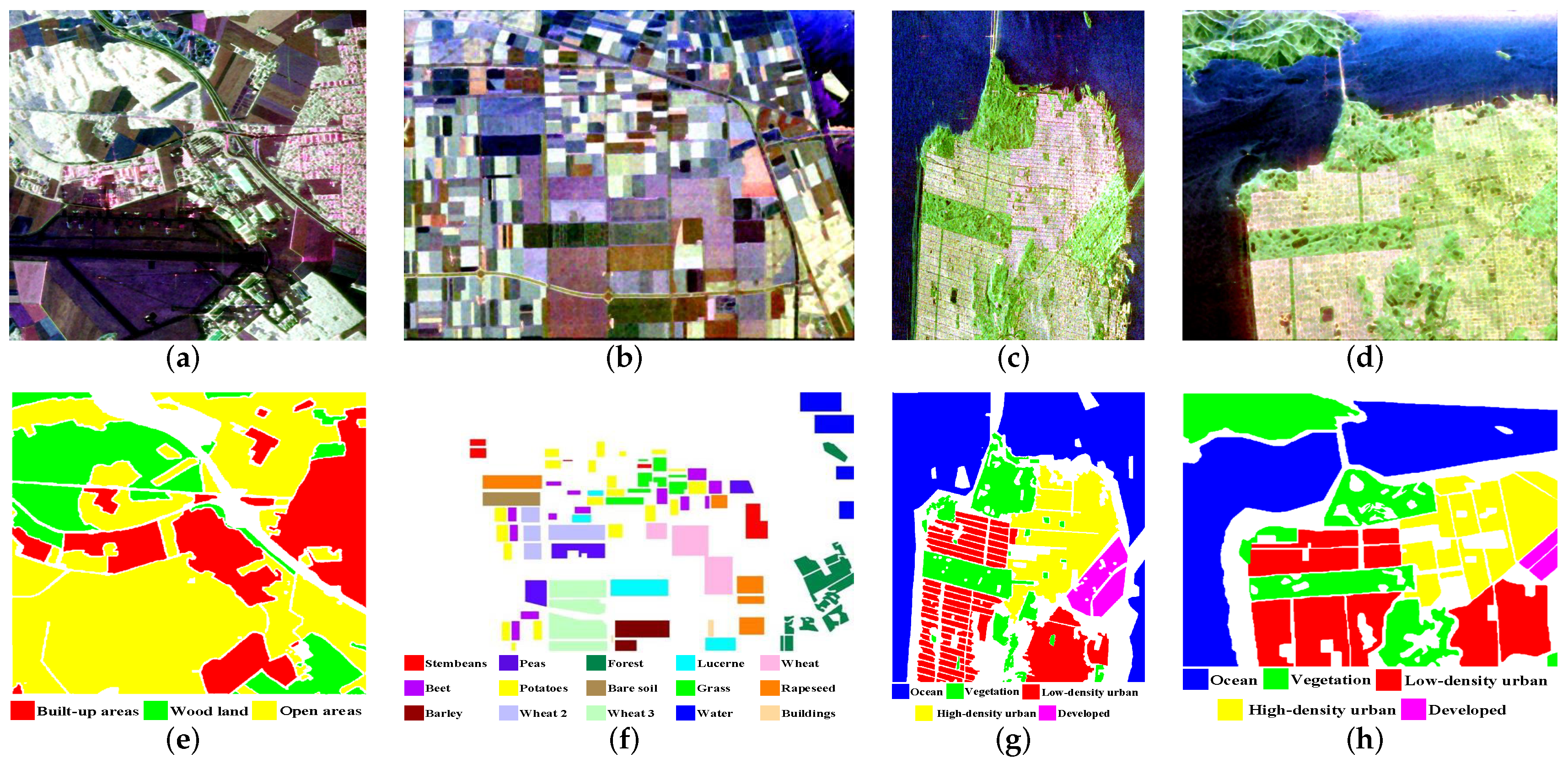
The rest of this paper is organized as follows: Section 2 provides a comprehensive overview of the methodologies employed in our proposed cross-level interaction graph U-Net (CLIGUNet). Section 3 presents the experiments and analyses conducted on four real PolSAR datasets. Finally, Section 4 summarizes the paper and provides insights into our future work.

2. Theory and Methodology

This paper proposes a PolSAR image segmentation model based on the cross-level interaction graph U-Net (CLIGUNet). First, Section 2.1 introduces PolSAR data preparation, where a coherency matrix is adopted as the input features. Next, Section 2.2 gives an overview of the network architecture and implementation of CLIGUNet. Then, Section 2.3 illustrates the motivation to propose the weighted max-relative spatial graph convolution inspired by deep GCNs [64], which incorporates the advantages of both image features in Euclidean space and polarimetric scattering similarity in the non-Euclidean graph domain, and thus enables the network parameters to generalize well on unseen graphs. Section 2.4 provides insight into the theoretical derivation of multi-scale dynamic graphs using k-NN and symmetric revised Wishart similarity, which is performed each iteration to map the image patches into the graph domain. Afterwards, in Section 2.5, a residual transformer with multi-head attention is proposed to interact between the bottleneck features and the graph structure across multiple resolutions. Finally, in Section 2.6, a deep supervision strategy is designated to fully utilize multi-scale information from neighbors in various scales, thus obtaining better segmentation results.

2.1. PolSAR Data Preparation

PolSAR platforms, by virtue of their ability to transmit and receive various polarimetric electromagnetic waves, can capture abundant scattering information from observed land covers, with each resolution cell in the fundamental SLC format being represented by a $2\times 2$ complex scattering matrix. Here, H and V represent the horizontal and vertical polarization modes, respectively. Subsequently, a $2\times 2$ complex polarimetric scattering matrix can be expressed as

$$S=\left[\begin{array}{cc}{S}_{HH}\hfill & S_{HV}\hfill \\ S_{VH}\hfill & S_{VV}\hfill \end{array}\right],$$

(1)

where the first and second subscripts denote the polarization modes of the received and transmitted electromagnetic waves, respectively.

According to the reciprocity theorem, $S_{HV}$ equals $S_{VH}$ in monostatic SAR systems. Consequently, the scattering vector in the Pauli basis can be written as

$$k=\frac{1}{\sqrt{2}}{\left[S_{HH}+S_{VV},S_{HH}-S_{VV},2S_{HV}\right]}^T$$

(2)

Therefore, the polarimetric coherence matrix T can be obtained by

$$T=〈k·k^H〉=\left[\begin{array}{ccc}{T}_{11}\hfill & T_{12}\hfill & T_{13}\hfill \\ T_{21}\hfill & T_{22}\hfill & T_{23}\hfill \\ T_{31}\hfill & T_{32}\hfill & T_{33}\hfill \end{array}\right]$$

(3)

2.2. Overall Network Architecture

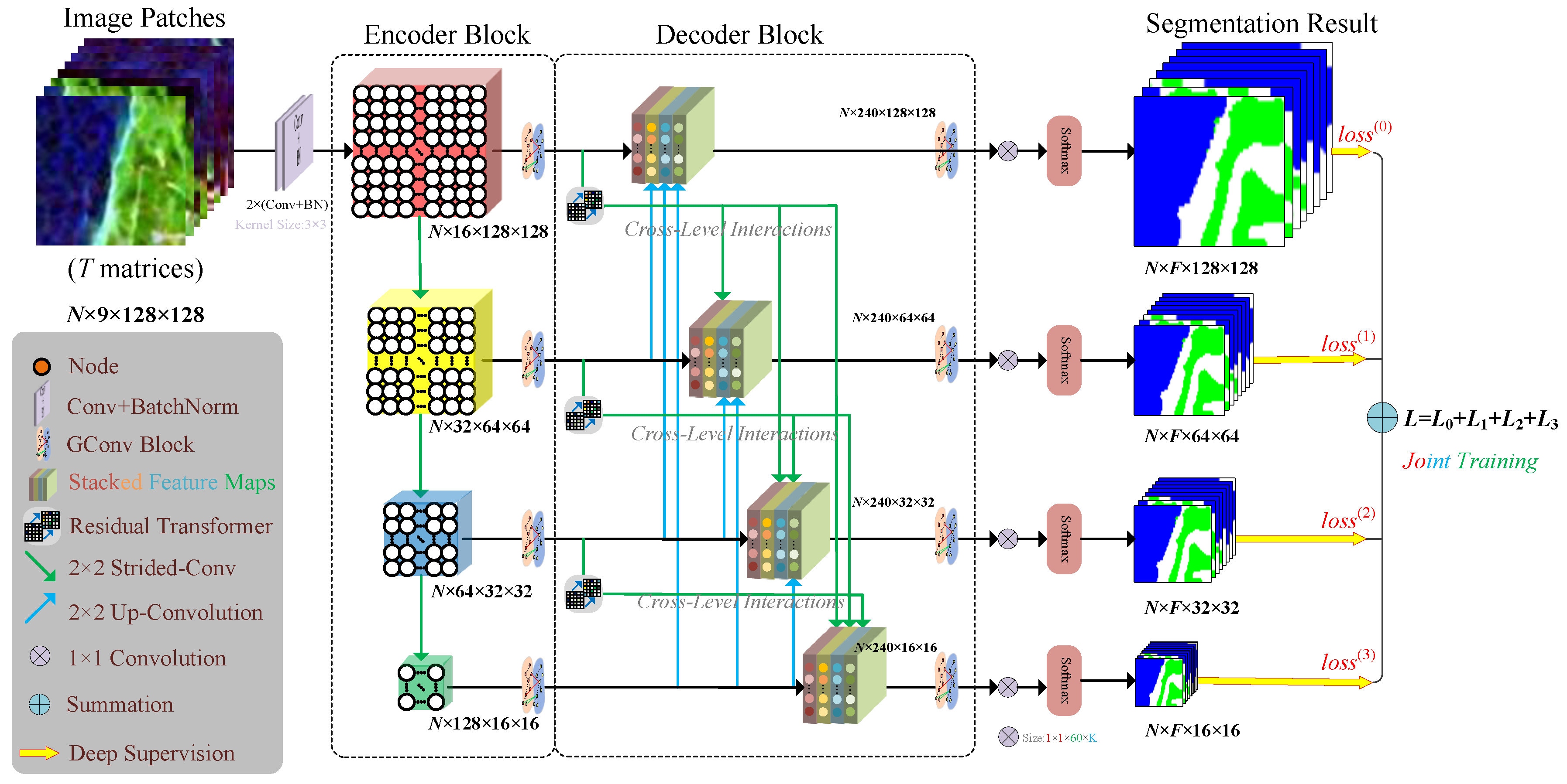
Figure 1 illustrates the hierarchical structure of the proposed CLiGUNet, which starts with an encoder backbone followed by a decoder sub-network. The detailed settings of the encoder block and decoder block are shown in

Table 1. Detailed settings of encoder block.

Encoder Components	Output Size	Layer (s)
Stem	$N_B\times L\times H/2\times W/2$	2 × (Conv + BatchNorm)
GConv + FFN	$N_B\times L\times H/2\times W/2$	$D=L,E=2,K=10$
Downsample	$N_B\times 2L\times H/4\times W/4$	$2\times 2$ Strided-Conv
GConv + FFN	$N_B\times 2L\times H/4\times W/4$	$D=2L,E=2,K=10$
Downsample	$N_B\times 4L\times H/8\times W/8$	$2\times 2$ Strided-Conv
GConv + FFN	$N_B\times 4L\times H/8\times W/8$	$D=4L,E=2,K=10$
Downsample	$N_B\times 8L\times H/16\times W/16$	$2\times 2$ Strided-Conv
GConv + FFN	$N_B\times 8L\times H/16\times W/16$	$D=8L,E=2,K=10$

and

Table 2. Detailed settings of decoder block.

Decoder Components	Output Size	Layer (s)
GConv + FFN	$N_B\times 15L\times H/16\times W/16$	$D=15L,E=2,K=10$
Upsample	$N_B\times 15L\times H/16\times W/16$	$2\times 2$ Up-Conv
GConv + FFN	$N_B\times 15L\times H/16\times W/16$	$D=15L,E=2,K=10$
Upsample	$N_B\times 15L\times H/8\times W/8$	$2\times 2$ Up-Conv
GConv + FFN	$N_B\times 15L\times H/8\times W/8$	$D=15L,E=2,K=10$
Upsample	$N_B\times 15L\times H/4\times W/4$	$2\times 2$ Up-Conv
GConv + FFN	$N_B\times 15L\times H/4\times W/4$	$D=15L,E=2,K=10$
Final Output	$N_B\times F\times H\times W$	$1\times 1$ Conv + Softmax

, respectively, where $N_B$ denotes the batch size, $H\times W$ denotes the input image size, D denotes the feature dimension, and L is the latent dimension (set to 16 in the experiments) of the stem component. E denotes the hidden dimension ratio, which means the convolutional layer number in FFN. K denotes the number of neighbors in the GC layer. The nine elements of the coherence matrix are used as the initial feature vector of each node in the input graph. Using two convolution layers with batch normalization, the input feature vectors are first mapped into a high-dimensional representation. To bridge the gap between image patches in the Euclidean grid structure and node feature representations in the graph domain, our CLIGUNet uses a k-NN approach [62] to recompute and generate the graph topology with learnable features in latent space in each iteration. To fully utilize the polarimetric scattering information of the PolSAR data, the edge weights of each graph are obtained based on the symmetric revised Wishart distance [50] and the thresholded weighting function.

The encoder section on the left comprises four stacked graph convolution (GC) blocks. Each GC block consists of a multi-layer neural network, including a weighted max-relative spatial graph convolutional layer with batch normalization and ReLU activation, as well as a feed-forward network (FFN) module. The FFN module serves to enhance the feature transformation capacity and alleviate the over-smoothing issue in the deeper graph convolutional layers. Then, a strided convolutional layer is applied to encode higher-level graph representations and reduce the input graph size. Afterwards, residual transformers are integrated to enhance the skip connections among the encoder features and decoder features. With the exception of the last convolution block, the feature representations from the preceding block are sub-sampled by a strided convolutional layer (depicted in green) before being passed to the next block. The input image size is set to $128\times 128$, where F denotes the number of land cover types and N represents the batch size.

The decoder section on the right consists of four decoder blocks. Each decoder block has a weighted max-relative spatial graph convolutional layer and a deconvolution layer, which aggregate information from neighbors and restore the graph to a higher resolution structure. The intra-connections among the stacked feature maps within the decoder sub-network are designed to facilitate the flow of information across different resolutions, enabling the network to capture both coarse-grained semantics and fine-grained details. Meanwhile, the interconnections between the encoder and decoder blocks help to establish skip connections, allowing the decoder to access and integrate multi-scale feature representations from the encoder, which helps in preserving spatial information and enhancing the performance of feature reconstruction. As a result, the skip connections above integrate feature maps from both lower- and same-scale layers of the encoder, as well as larger-scale feature maps from the decoder. Subsequently, softmax normalization is applied after the last GC block at each resolution to produce the segmentation result for each concatenated feature map, which comes in the form of multi-class probabilities for each image patch. After that, the dice loss and cross-entropy (CE) at each scale are summed up to perform deep supervision. Finally, PolSAR image segmentation is performed by taking the column number with the highest probability value and merging the results of all image patches.

2.3. Weighted Max-Relative Spatial Graph Convolution

Compared with CNNs, GCNs are capable of extracting more extensive features by aggregating node features from their neighborhood. The recent literature has witnessed the application of spectral GCNs in PolSAR image classification tasks [7,53]. However, spectral GCNs are often designed to operate on a specific graph structure with a fixed adjacency matrix, which makes it struggle to generalize well on unseen graphs with a different topology. This limitation arises because the feature representation in the spectral domain is closely related to the graph Laplacian [66]. Thus, any change in the adjacency matrix can substantially impact the spectral characteristics. Spatial GCN exhibits better adaptability to varying graph structures and is exceptionally well-suited to deal with this issue. This is because spatial convolutional operations depend on the local neighborhood, making the model more robust to changes in the graph topology.

Suppose the PolSAR dataset is divided into N patches, and each patch is flattened into a feature vector. Then, the graph nodes can be described as $X=\left[x_1,x_2,\cdots ,x_N\right]$. Then, the k-NN [64] is utilized to establish connections between nodes. Therefore, the graph representation of each image patch can be denoted as $\mathcal{G}=(\mathcal{V},\mathcal{E})$, where $\mathcal{V}$ denotes the graph nodes and $\mathcal{E}$ denotes the graph edges.

For the graph representation $\mathcal{G}=G\left(X\right)$ and the input features X, a spatial graph convolutional layer can be applied to aggregate node features from its neighbor nodes, as follows:

$$\begin{array}{cc}\hfill {\mathcal{G}}^{\prime }& =F(\mathcal{G},\mathcal{W})\hfill \\ \hfill & =\mathrm{Update}\left(\mathrm{Aggregate}\left(\mathcal{G},W_{\mathrm{agg}}\right),W_{\mathrm{update}}\right),\hfill \end{array}$$

(4)

where $W_{\mathrm{update}}$ and $W_{\mathrm{agg}}$ are the learnable weights of the update and aggregation operations, respectively. The Aggregate operator aggregates the neighboring node features, and the Update operator merges the aggregated feature representation as follows:

$$x_i^{\prime }=h\left(x_i,g\left(x_i,\mathcal{N}\left(x_i\right),W_{\mathrm{agg}}\right),W_{\mathrm{update}}\right),$$

(5)

where $\mathcal{N}\left(x_i\right)$ are the neighboring nodes of $x_i$.

Inspired by [64], weighted max-relative graph convolution $X^{\prime }=$$\mathrm{GraphConv}\left(X\right)$ is proposed to fully leverage the edge weights derived from the PolSAR scattering characteristics, which can be written as:

$$\begin{array}{cc}\hfill & g(·)=x_i^{″}=\left[x_i,max\left(\left\{{\omega }_{i,j}{x}_j-x_i\mid j\in \mathcal{N}\left(x_i\right)\right\}\right],\right.\hfill \\ \hfill & h(·)=x_i^{\prime }=x_i^{″}{W}_{\mathrm{update}}+b,\hfill \end{array}$$

(6)

where ${\omega }_{i,j}$ is the edge weight between node i and node j and b is the bias term.

To enrich the feature diversity of spatial graph convolution, the multi-head update operation is adopted in multiple feature subspaces by splitting the aggregated feature ${\mathbf{x}}_i^{″}$ into H heads, which is set to 4 by default. Then, these heads are updated with different weights and concatenated to obtain the final representation, as follows:

$$x_i^{\prime }=\left[\mathrm{head}{ }^1{W}_{\mathrm{update}}^1+b^1,\mathrm{head}{ }^2{W}_{\mathrm{update}}^2+b^2,\cdots ,\mathrm{head}{ }^h{W}_{\mathrm{update}}^h+b^H\right],$$

(7)

where $b^i$ denotes the bias term of the ith attention head ($i=1,2,\cdots ,H$).

To alleviate over-fitting and thus enhance the generalization ability, a DropPath layer [67] has been applied to stochastically deactivate some of the skip connections during training. Thus, the final expression of the graph convolution module can be written as:

$$Y=DropPath\left(GELU\left(\mathrm{GraphConv}\left(X{W}_{\mathrm{in}}\right)\right)W_{\mathrm{out}}+b_{\mathrm{out}}\right)+X,$$

(8)

where GELU is the Gaussian error linear unit [68], which is differentiable in all ranges and allows to have gradients in the negative range to prevent vanishing gradients. X denotes the input features, $b_{\mathrm{out}}$ is the bias term, and $W_{\mathrm{in}}$ and $W_{\mathrm{out}}$ are the fully connected (FC) layer weights for input and output, respectively.

To further boost the feature transformation capability and relieve the over-smoothing in deeper layers, a feed-forward module (FFN) is applied after graph convolution. It consists of a multi-layer structure with two FC layers, i.e.,

$$Z=GELU\left(Y{W}_1+b_1\right)W_2+b_2+Y,$$

(9)

where Z is the output of the graph convolution module, $W_1$ and $W_2$ are FC layer weights, and $b_1$ and $b_2$ are the bias terms.

2.4. Multi-Scale Dynamic Graphs

After the application of a sliding window to slice the PolSAR dataset into image patches, our CLIGUNet utilizes a k-NN approach [64] to generate the graph topology at each scale. This strategy constructs a graph from an image patch by first representing each pixel in the patch as a node in the graph. Then, the k-nearest neighbors of each node in the feature space are selected to form the edges between the central pixel and its k-nearest neighbors. Based on the Euclidean distance, this graph representation captures the local spatial relationships within the image patch, thus facilitating effective feature extraction and contextual information modeling in each iteration.

Afterwards, the k-NN approach encodes connected pixel groups in the ith PolSAR image patch into an adjacency matrix $A_i(i=1,\dots ,N)$, with N denoting the batch size of CLIGUNet. To evaluate the relative importance of neighboring nodes, the symmetric revised Wishart distance is applied to derive multi-scale weighted adjacency matrices $W_i(i=1,\dots ,N)$, as described below.

2.4.1. Weighted Adjacency Matrix

Our CLIGUNet focuses on weighted, connected, undirected graphs $\mathcal{G}=\left\{\mathcal{V},\mathcal{E},W\right\}$, which are made up of node sets $\mathcal{V}$, edge sets $\mathcal{E}$, and a weighted adjacency matrix W. The difference between the binary adjacency matrix A and W lies in their edge weights, which can help the graph convolutional layers to address the neighbors with stronger relevance.

To alleviate the computational cost, sliding windows are utilized to slice the Pauli RGB images into patches, where each pixel serves as a graph node. However, the revised symmetric Wishart distance can take both negative and positive values, which cannot be directly applied for graph construction. To cope with this problem, a thresholded Gaussian kernel weighting function [69] normalizes the distance to a similarity value between 0 and 1. The pair-wise similarity, which indicates the edge weight of the neighboring node i and node j, can be derived as:

$$\begin{array}{c}\begin{array}{c}\hfill W_{i,j}=\left\{\begin{array}{cc}\exp \left(-d^2\left(i,j\right)/\phantom{d^2\left(i,j\right)2{\sigma }^2}2{\sigma }^2\right)& whene\left(i,j\right)=1\\ 0& whene\left(i,j\right)=0,\end{array}\right.\end{array}\end{array}$$

(10)

where $e(i,j)$ denotes the connectivity between node i and node j ($i\ne j$), which is equal to 1 for neighboring pixels, $d\left(i,j\right)$ represents the Euclidean distance between the neighboring nodes, and $\sigma$ represents the Gaussian kernel standard deviation.

Recent research has validated the effectiveness of the symmetric revised Wishart distance [7,49,53,59,70] in assessing the dissimilarity among complex coherency matrices. It is defined as:

$$d_{SRW}\left(T_i,T_j\right)=\frac{1}{2}tr\left(T_i{T}_j^{-1}+T_j{T}_i^{-1}\right)-3,$$

(11)

where $T_i$ and $T_j$ represent the coherence matrices for pixel i and pixel j, respectively.

Derived from the weighting function in (10) and the distance measure in (11), our paper constructs the weighted adjacency matrix as:

$$W_{ij}^{\mathrm{SRW}}=\left\{\begin{array}{cc}\exp \left(\frac{-d_{\mathrm{SRW}}^2\left(T_i,T_j\right)}{2{\sigma }_i{\sigma }_j}\right)& whene(i,j)=1\\ 0& whene(i,j)=0,\end{array}\right.$$

(12)

where $e\left(i,j\right)$ indicates the node pair connectivity, ${\sigma }_i$ denotes the local scaling parameter [48] defined as the median distance between the current node i and its neighborhood, and $d_{\mathrm{SRW}}$ denotes the symmetric revised Wishart distance between two mean coherence matrices.

2.4.2. Graph Connectivity Augmentation via Graph Power

The kth power of graph ${\mathbb{G}}^k$ is applied to avoid possible isolated nodes and increase graph connectivity, where k indicates that the neighbors are within k hops from the current node. To sample the augmented graph with better connectivity, a self-loop is applied to renormalize the adjacency matrix $\widehat{W}=W+I$. Since our proposed network deploys a graph convolutional layer before strided convolution to aggregate the features of first-order neighbors, it is safe to assume the graph order k as 2, thus obtaining the second power of the graph, as follows:

$$\begin{array}{cc}\hfill & A^{\mathcal{l}+1}=A_l^2(\mathrm{idx},\mathrm{idx})\hfill \\ \hfill & A_l^2=A^{\mathcal{l}}{A}^{\mathcal{l}},\hfill \end{array}$$

(13)

where $A^2\in {\mathbb{R}}^{N\times N}$ denotes the second power of the adjacency matrix $A^{\mathcal{l}}$ on layer ℓ, $idx$ ranges from 1 to N, and N denotes the batch number in graph $\mathbb{G}$.

Considering that the feature vector of the current node itself should play a more important role, a self-loop is applied to renormalize the adjacency matrix A, thus obtaining an augmented graph $\widehat{A}=A+I$ with better connectivity.

2.4.3. Weighted Graphs and Ground Truth in Multiple Scales

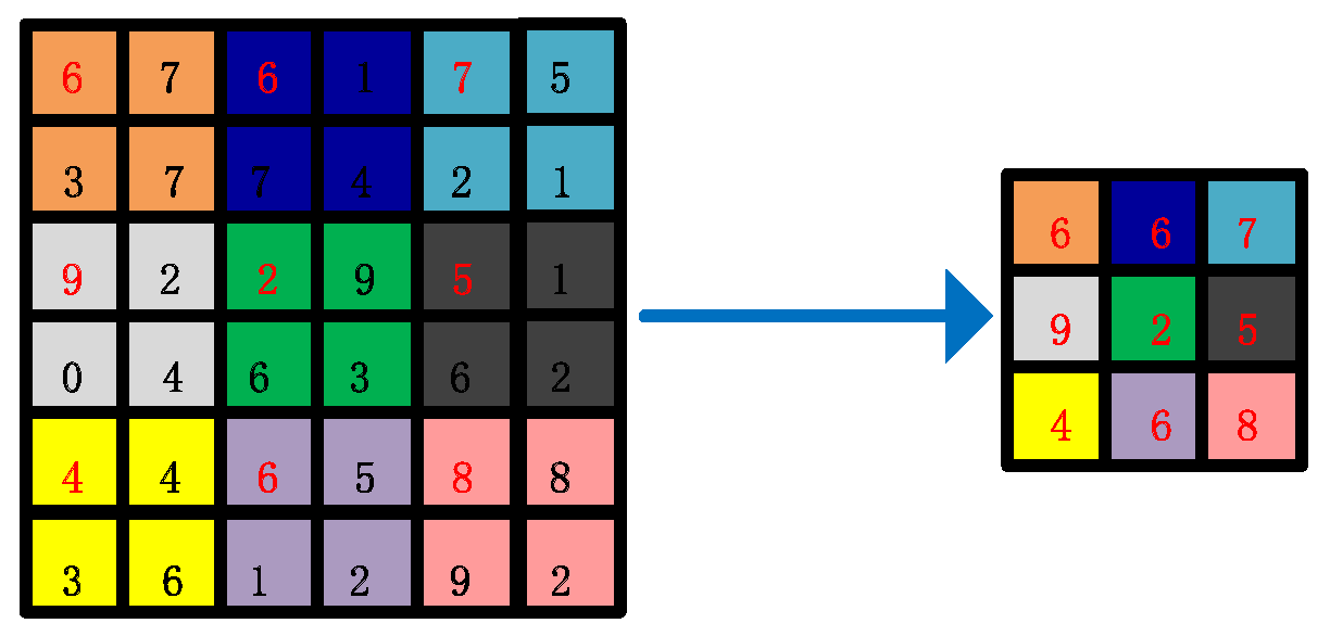
The main advantage of our CLIGUNet lies in its ability to learn node features from multiple scales weighted graphs. In the data preparation stage, the dense weighted adjacency matrices ${\widehat{W}}_n^l$ are saved in advance, assuming that all nodes are interconnected with each other, where n ($n=1,2,\cdots ,N$) is the patch number and l ($l=1,2,\cdots ,L$) denotes the lth scale. The multi-scale labels of each image patch are obtained by taking the first value in the upper left corner every $2^i\times 2^i(i=0,1,2,3)$ pixels, as shown in Figure 2, where the label map with 36 pixels is coarsened to 9 pixels. During the training process, the binary adjacency matrices $A_n^l$ are obtained by searching the k-nearest neighbors of each node. Afterwards, the weighted adjacency matrices $W_n^l$ can be calculated by taking the dot products of ${\widehat{W}}_n^l$ and $A_n^l$.

2.5. Cross-Level Interactions with Residual Transformer

We introduce a novel approach to the integrated multi-scale features by leveraging the concept of cross-level interactions with residual transformers to address the relative importance of node features at different scales. Drawing inspiration from the graph integration module [7,53] and the bottleneck attention module [71,72], a weighted max-relative spatial graph convolution module is constructed at each resolution, facilitating the extraction of features at the local scale. Then, pooling and unpooling layers are employed to align feature vectors across scales. Afterwards, node feature representations in the decoder are obtained by concatenating deep features from all scales, utilizing residual connections between encoders and corresponding decoder blocks to transfer spatial information for better performance. Finally, in each resolution, the feature maps from multiple scales are concatenated together and fed into a graph convolution layer to generate the segmentation result for the corresponding scale and calculate the total loss in this batch.

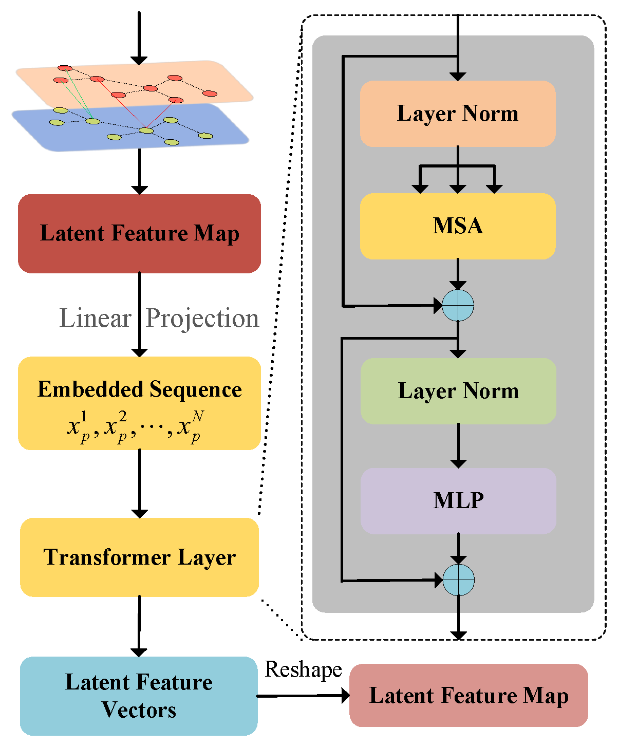
The residual transformer module is a key component in our architecture, leveraging self-attention to capture the global relationships between the encoder and decoder, as shown in Figure 3. This mechanism, crucial for learning the relative importance of each channel, is enhanced by residual connections across resolutions. Similar to other transformer modules, our residual transformer incorporates multi-head self-attention (MSA), multi-layer perceptron (MLP), and layer normalization (LN). Compared with CNNs, which rely on convolutional and pooling layers for feature extraction from local information, the transformer excels in extracting global features. By employing the attention mechanism, the model learns long-range dependencies, enabling the encoding of patches with global contextual information. This capability enables to capture relationships between ordered patches, ultimately enhancing the segmentation performance at each resolution.

To preserve spatial location information among input patches, the latent feature map X is flattened into a patch sequence $\left\{x_p^i\in {\mathbb{R}}^{P^2·C}\mid i=1,\dots ,N_s\right\}$, where $N_s=\frac{HW}{P^2}$ is the input sequence length, which equals the number of image patches in a single batch, P is the patch size, C is the number of channels, and H and W are the height and width of the input image patch, respectively. Using a trainable linear projection, these vectorized patches ${\mathbf{x}}_p$ are then projected into a latent feature embedding subspace, which can be written as:

$$z_0=\left[x_p^{1}E;x_p^{2}E;\cdots ;x_p^{N}E\right]+E_{pos},$$

(14)

where $E_{pos}\in {\mathbb{R}}^{N\times D}$ represents the position embedding and E denotes the patch embedding projection.

Let us assume that each residual transformer module consists of L layers of MSA and MLP. The output of the ℓ-th layer can be obtained as:

$$\begin{array}{c}{z}_l^{\prime }=\mathrm{MSA}\left(\mathrm{LN}\left(z_{l-1}\right)\right)+z_{l-1},l=1,2\dots ,L\end{array}$$

(15)

$$\begin{array}{c}{z}_l=\mathrm{MLP}\left(\mathrm{LN}\left(z_l^{\prime }\right)\right)+z_l^{\prime },l=1,2\dots ,L\end{array}$$

(16)

where the MLP in (16) consists of two FC layers and a GELU activation function, and ${\mathbf{z}}_l$ denotes the latent feature representation in the ℓ-th layer.

Then, the three learnable weight matrices composed of query $Q\in {\mathbb{R}}^{D_q}$, key $K\in {\mathbb{R}}^{D_k}$, and value $V\in {\mathbb{R}}^{D_v}$, are introduced to perform multiplication with the input image representation sequence ${\mathbf{z}}_l$, written as $[Q,K,V]=Z·WQKV$, where $W_{QKV}\in {\mathbb{R}}^{d\times 3D_k}$, $D_q$, $D_k$, and $D_v$ denote the feature dimension of query, key, and value, respectively.

The relative importance of each patch in the input image representation sequence ${\mathbf{z}}_l$ can be obtained by computing the dot product between the Q-vector and the K-vectors. After that, a softmax function is applied to calculate the V values. Finally, each patch embedding vector is multiplied by the V values to address the effective representations with a higher attention score, as

$$\mathrm{Attention}(Q,K,V)=\mathrm{softmax}\left(\frac{Q{K}^T}{\sqrt{D_k}}\right)V$$

(17)

During the MSA phase, multiple dot-product attention is performed by iterating (17) h times. Afterwards, each parallel attention map ${\mathrm{Head}}_i$ is concatenated as follows:

$$\mathrm{MultiHead}(Q,K,V)=\mathrm{concat}\left({\mathrm{Head}}_1,\cdots ,{\mathrm{Head}}_H\right)W^O$$

(18)

$${\mathrm{Head}}_i=\mathrm{Attention}\left(Q{W}_i^Q,K{W}_i^K,V{W}_i^V\right),i=1,\dots ,H$$

(19)

where $W^O\in {\mathbb{R}}^{h\times D_v\times \mathrm{d}}$ denotes the relative importance of each attention head, and $W_i^Q\in {\mathbb{R}}^{\mathrm{d}\times D_q},W_i^K\in {\mathbb{R}}^{\mathrm{d}\times D_k},W_i^V\in {\mathbb{R}}^{\mathrm{d}\times D_v}$ are the three learnable attention weights for the ith head.

As illustrated in Figure 3, both MSA and MLP utilize LN layers for normalization and skip-connections for better gradient flow and alleviate the vanishing gradient problem in the transformer module. The MSA block extracts rich semantic features from a patch sequence by capturing data correlations and establishing dependencies among various features. Then, the weights derived from MSA are directed to the MLP layer. Layer normalization [73] is applied before the MLP layer to accelerate training and mitigate the challenges posed by a vanishing gradient. The MLP layer consists of two FC layers, with the nonlinearity between the layers being activated by the GELU function.

2.6. Joint Training of Multi-Scale Graphs

Taking inspiration from deeply supervised networks (DeepSup) [74], this paper leverages multi-scale side outputs, multi-scale labels, and deep supervision to enhance the discriminative capability of feature maps across multiple resolutions and alleviate potential issues with gradient vanishing.

In contrast to conventional U-Nets and graph U-Nets, our CLIGUNet not only incorporates feature maps from different hierarchical levels via strided convolution and transposed convolution, but also produces the segmentation map at each resolution. Figure 1 depicts the process of collecting effective representations at all resolutions using a deep supervision training strategy, employing side outputs across multiple scales. This technique facilitates model pruning and yields improved or comparable performance, as opposed to relying solely on the top layer’s output to calculate the loss function.

By integrating multi-scale residual connections in the decoder, our CLIGUNet produces feature maps and segmentation results across each semantic level, which are the foundational conditions for implementing deep supervision.

The total loss function is composed of four parts, where each part is a combination of both the dice loss and CE loss, as follows:

$$\mathcal{L}=\sum _{l=0}^{L=3}{\mathcal{L}}^{\left(l\right)}$$

(20)

$${\mathcal{L}}^{\left(l\right)}(y^{\left(l\right)},{\widehat{y}}^{\left(l\right)})=-\frac{1}{N_B}\sum _{i=1}^N\left\{\frac{2y_i^{\left(l\right)}{\widehat{y}}_i^{\left(l\right)}}{y_i^{\left(l\right)}+{\widehat{y}}_i^{\left(l\right)}}+y_i^{\left(l\right)}\ln {\widehat{y}}_i^{\left(l\right)}\right\}+\lambda {∥w∥}^2,$$

(21)

where ${\mathcal{L}}^{\left(l\right)}$ represents the loss value of the lth side output, $N_B$ indicates the batch size, and $y_i^{\left(l\right)}$ and ${\widehat{y}}_i^{\left(l\right)}$ denote the flattened ground truth (class labels) and probability output (predictions) of the ith image patch at the lth scale, respectively. ${∥w∥}^2$ denotes the $L_2$-norm regularization term, with the regularization strength $\lambda$ being a hyperparameter that adjusts the tradeoff between having a low training loss and having low weights.

3. Experimental Results and Discussion

In this section, four PolSAR datasets are used to evaluate the performance of our proposed CLIGUNet in PolSAR image segmentation tasks within the same dataset and across datasets with similar land covers. Section 3.1 gives a brief introduction to the PolSAR datasets and parameter settings. Section 3.2 presents the ablation studies to investigate the effectiveness of weighted max-relative spatial graph convolution, multi-scale dynamic graphs, cross-level interactions with residual transformers, and the deep supervision training strategy. Section 3.3 and Section 3.4 demonstrate the effectiveness of our CLIGUNet by comparing its segmentation results with other state-of-the-art networks, including SVM [27], UNet [41], WDBN [33], WCAE [38], CV-CNN [40], MDPL-SAE [37], GraphCNN [75], and MEWGCN [7], where GraphCNN and MEWGCN are semi-supervised methods with graph convolution, while the others are supervised methods.

3.1. Dataset Description and Experiment Settings

Figure 4 illustrates the four PolSAR datasets used to evaluate the classification performance of our CLIGUNet. These datasets include different types of terrains and land covers, including ocean, forest, agriculture areas, and buildings. To eliminate the negative impact of imbalanced datasets on the experiments, the number of training samples is set the same for each class. In the pre-processing stage, a refined Lee filter [76] is applied on all these datasets to reduce speckle noise, with the window size set to $7\times 7$ for all the comparative tests. Detailed information about these PolSAR datasets can be found in

Table 3. Information about PolSAR datasets used in the experiments.

Dataset Name	Radar	Band	Year	Resolution	Polarimetric Type	Size	Classes
Oberpfaffenhofen	E-SAR	L	1991	3 m × 2.2 m	Full polarimetric	1300 × 1200	3
Flevoland	AIRSAR	L	2010	12.1 m × 6.7 m	Full polarimetric	750 × 1024	15
San Francisco RS-2	RADARSAT-2	C	2008	10 m × 5 m	Full polarimetric	1800 × 1380	5
San Francisco AIRSAR	AIRSAR	L	1989	12.1 m × 6.7 m	Full polarimetric	900 × 1024	5

.

3.1.1. Oberpfaffenhofen Dataset

The Oberpfaffenhofen dataset was recorded by ESAR L-band radar over Oberpfaffenhofen in Germany in 1991. The image has a size of $1300\times 1200$. Its Pauli RGB composition is shown in Figure 4a. Figure 4e shows the ground truth of this dataset, which consists of woodland, open areas, and built-up areas.

3.1.2. Flevoland Dataset

This multi-look benchmark dataset has been widely employed in evaluating the performance of PolSAR image classification approaches. It was acquired by NASA/JPL AIRSAR L-band radar over the agriculture area of the Dutch province of Flevoland in 2010. The Pauli RGB image has a size of $750\times 1024$, and consists of 15 different classes, including forests, crops, buildings, and water, with its ground truth illustrated in Figure 4f.

3.1.3. San Francisco Datasets

The RADARSAT-2 San Francisco (SF-RS2) dataset was acquired by RADARSAT-2 C-band radar over San Francisco in 2008. This dataset has a size of $1800\times 1380$, which consists of five classes, including ocean, vegetation, low-density urban, high-density urban, and developed. The Pauli RGB image and ground truth are shown in Figure 4c and Figure 4g, respectively.

The AIRSAR San Francisco (SF-AIRSAR) dataset was recorded by AIRSAR L-band radar in 1989. This dataset has a size of $900\times 1024$, with its Pauli RGB image and ground truth shown in Figure 4d and Figure 4h, respectively.

As these two San Francisco datasets share similar land covers, they are used together to assess the capability to generalize across PolSAR datasets with similar scenes.

3.1.4. Experimental Settings

In order to strike a balance between better representation learning and less computational cost, the sliding window size and step size are set as $128\times 128$ and 25 for both CLIUNet and UNet [41], respectively. For the overlapping regions of the image patches, the final classification result is determined by majority voting. After the PolSAR image is split into patches, the coherence matrix vectors in each patch are rescaled using z-score normalization. Finally, rotation and flips are applied to each image patch to augment the datasets.

As a matter of experience, the initial neighboring pixel number for k-NN is set to 10 in the experiments. This is because a too few number of neighbors is insufficient for developing an effective graph representation, thus resulting in inadequate feature learning, slow convergence, and coarse segmentation results. On the contrary, larger neighbor numbers provide more refined texture details at the cost of decreased computational efficiency. Moreover, the performance of k-NN is also affected by the symmetry of the adjacency matrix, which, in turn, is associated with the graph structure and significantly impacts the classification results. As a solution, the weighted adjacency matrix W is constructed and flipped. This can be achieved by taking the maximum elements of W and $W^{\prime }$ in the final procedure.

Our CLIGUNet is implemented with PyTorch 1.10.0. The experiments are conducted using a GeForce RTX 3090 GPU and an AMD Ryzen 9 5900X CPU. A Xavier uniform initializer [77] is used to initialize the layer weights and biases. Early stopping is implemented as a preventive measure against overfitting, which stops the training process if the validation loss fails to decrease for a consecutive span of 20 epochs. The suggested learning rates and droppath rates for CLIGUNet are $2\times {10}^{-3}$∼$5\times {10}^{-2}$ and 0.1∼0.25, respectively. The Adam SGD optimizer is applied to minimize the total loss, with the $L_2$-norm regularization strength $\lambda$ fixed at $1\times {10}^{-4}$.

Table 4. Training+validation data used for the different methods in the experiments.

Method	Flevoland	SF-RS2	SF-AIRSAR	SF-AIRSAR→SF-RS2
SVM [27]	9%	2%	2%	2%
UNet [41]	9% + 1%	2% + 1%	2% + 1%	2% + 1%
WCAE [38]	5% + 1%	10% + 1%	—	—
CV-CNN [40]	9% + 1%	2% + 1%	2%+1%	2% + 1%
MDPL-SAE [37]	9%	2%	—	—
WDBN [33,38]	5%	10%	2%	2%
GraphCNN [75]	5%	—	—	—
MWGCN [7]	4% + 1%	1.5% + 0.5%	1.5% + 0.5%	1.5% + 0.5%
CLIGUNet	4% + 1%	1.5% + 0.5%	1.5% + 0.5%	1.5% + 0.5%

shows the percentage of ground truth samples used for the training and validation of the comparative methods. Note that our CLIGUNet uses the smallest number of ground truth samples, as bolded in the last row of Table 4. The em dashes indicate the experiments not implemented by the original reference works.

The experiments described in Section 3.3, Section 3.4 and Section 3.5 show that our CLIGUNet outperforms other PolSAR image classification approaches on the Flevoland dataset, the SF-RS2 dataset, and the SF-AIRSAR dataset. SVM is selected as the representative for traditional methods, while UNet is used as the baseline for deep learning approaches. WCAE and MDPL-SAE are chosen as the variants of AE. CV-CNN, WDBN, and MWGCN are used as the representatives of CNNs, DBNs, and GCNs, respectively.

3.2. Ablation Studies

In this section, the ablation studies carried out on the Oberpfaffenhofen dataset to analyze the benefits of our mechanisms are described, which are proposed in Section 2.3, Section 2.4, Section 2.5 and Section 2.6. These mechanisms are evaluated with four variants of our CLIGUNet, namely, ${\mathrm{CLIGUNet}}_{ws}$, ${\mathrm{CLIGUNet}}_{dg}$, ${\mathrm{CLIGUNet}}_{rt}$, and ${\mathrm{CLIGUNet}}_{ds}$, that one at a time introduce weighted spatial graph convolution ($ws$), dynamic graphs ($dg$), residual transformer modules ($rt$), and deep supervision ($ds$). The overall accuracy and class-by-class accuracies are chosen to validate the effectiveness of the different variants, with the best segmentation maps obtained by conducting five repeated experiments on each training set and validation set (10 random splits in each case). Figure 5 shows the best segmentation results provided by the six variants.

Table 5. Classification accuracies and running time of CLIGUNet variants in the ablation study (provided by % and s).

Class	No Mechanism	${\mathrm{CLIGUNet}}_{\mathit{wm}}$	${\mathrm{CLIGUNet}}_{\mathit{dg}}$	${\mathrm{CLIGUNet}}_{\mathit{rt}}$	${\mathrm{CLIGUNet}}_{\mathit{ds}}$	CLIGUNet
Built-up	82.36 ± 5.57	85.39 ± 4.24	85.73 ± 4.36	84.36 ± 3.28	88.62 ± 2.85	88.93 ± 1.78
Wood	83.27 ± 5.72	86.94 ± 4.85	92.56 ± 4.51	92.48 ± 2.72	91.31 ± 2.63	95.98 ± 1.53
Open	90.82 ± 4.31	93.83 ± 3.88	91.71 ± 4.14	96.87 ± 2.53	96.93 ± 2.14	96.95 ± 1.95
OA	87.63 ± 5.16	89.32 ± 4.47	91.06 ± 4.28	92.72 ± 2.85	93.04 ± 2.48	93.92 ± 1.84
$T_{train}$	161.55 ± 17.86	181.74 ± 12.43	217.63 ± 18.05	195.72 ± 18.49	183.17 ± 15.57	286.74 ± 16.82
$T_{pred}$	46.54 ± 1.81	48.27 ± 1.63	53.16 ± 1.16	58.74 ± 1.95	55.62 ± 1.79	67.03 ± 2.14

reports the mean values and standard deviation values of both the overall accuracy and class-specific accuracy of each CLIGUNet variant.

Figure 5a shows the segmentation map of CLIGUNet with no mechanism, which is used as the baseline to analyze the improvements. Figure 5b,c illustrate the best results with ${\mathrm{CLIGUNet}}_{ws}$ and ${\mathrm{CLIGUNet}}_{dg}$. Their improvements are not easy to identify, since the segmentation maps are rough with a large number of misclassified pixel groups in the maps obtained. Employing residual transformer modules and graph deep-supervision, Figure 5d,e present smoother classification results. The removed misclassified spots, together with the average accuracy values in Table 5, indicate that both the residual transformer modules and deep-supervision contribute more to learning effective feature representations than the weighted max-relative spatial graph convolution and dynamic graphs. Figure 5f presents the best segmentation result of complete CLIGUNet, which considers all the above methods at the same time.

From the accuracy mean values and standard deviation values in Table 5, one can observe that each mechanism helps in improving and stabilizing the classification performance. The mean accuracy values of ${\mathrm{CLIGUNet}}_{ws}$ and ${\mathrm{CLIGUNet}}_{dg}$ in the third and fourth columns indicate that initializing the weighted graph edges and revising inaccurate graph representations can make a significant impact on the classification results. The standard deviation values of ${\mathrm{CLIGUNet}}_{rt}$ and ${\mathrm{CLIGUNet}}_{ds}$ in the fifth and sixth columns are smaller than those of ${\mathrm{CLIGUNet}}_{wm}$ and ${\mathrm{CLIGUNet}}_{dg}$, thanks to the higher-order adjacency matrices and multi-scale labels with larger receptive fields, which not only boosts the classification accuracy, but also helps in obtaining more stable segmentation results. Furthermore, one can also observe the additional training and prediction time brought by each component in the last two rows of Table 5. Considering the significant improvement in segmentation performance, it is worth paying the price for these mechanisms.

3.3. Results on Flevoland Dataset

On the Flevoland dataset, the effectiveness of our CLIGUNet is demonstrated against SVM and seven other deep learning methods. Figure 6b shows that SVM fails to properly interpret the PolSAR image well, especially in the red squares. This is mainly due to the incapacity of SVM to capture regional information, which can help to learn more effective feature representations. The classification map in Figure 6c shows the poor performance of U-Net on this PolSAR dataset. As highlighted in the red squares, UNet struggles to discriminate land covers such as stembean, rapeseed, wheat 1, wheat 2, peas, and buildings. This challenge arises due to the over-smoothing effect in classical UNets. The classification map of WCAE in Figure 6d shows a large number of misclassified regions. Figure 6e,f illustrate that CV-CNN and WDBN can produce much better maps than previous methods. Figure 6g shows that MDPL-SAE generally performs well, except for the speckle noise in the red rectangles. Figure 6h,i illustrates that GraphCNN and MWGCN demonstrates better performance in the vast majority of regions. Finally, Figure 6j presents the best classification map of our CLIGUNet, where few misclassified areas can be observed. While our proposed CLUGUNet outperforms other approaches, the misclassified land covers in the gray rectangles suggest potential improvements for our future research.

Table 6. Classification accuracies and running time of different methods on Flevoland dataset (provided by % and s).

Class	SVM	U-Net	WCAE	CV-CNN	WDBN	MDPL-SAE	GCNN	MWGCN	CLIGUNet
Stem beans	90.71	93.33	88.09	99.62	96.71	98.45	98.76	99.07	99.85
Peas	85.23	99.37	96.11	98.38	98.68	98.46	99.62	96.58	99.78
Forest	96.05	99.10	97.89	95.93	96.45	99.37	99.93	96.31	99.89
Lucerne	94.89	97.55	97.42	99.34	98.47	97.95	97.66	99.88	99.94
Wheat	82.87	88.74	89.71	94.84	97.67	99.22	99.82	99.81	99.65
Beet	95.48	97.46	98.30	98.09	98.14	97.51	99.60	96.55	99.88
Potatoes	93.88	100.00	95.62	99.18	98.28	97.69	99.83	96.34	99.85
Bare soil	82.83	98.13	97.42	94.57	97.34	99.65	100.00	99.92	99.93
Grass	87.07	96.65	88.62	92.95	95.39	92.75	98.35	99.90	99.92
Rapeseed	90.02	99.72	77.83	95.69	95.90	97.66	98.21	97.89	99.26
Barley	73.30	92.91	99.27	91.80	99.49	98.84	97.44	99.80	99.88
Wheat2	81.38	86.08	88.11	96.30	94.79	98.56	92.52	96.14	99.56
Wheat3	88.07	59.86	98.05	96.60	98.55	99.04	97.93	98.70	99.39
Water	49.92	89.62	93.46	99.40	99.90	99.77	100.00	100.00	100.00
Buildings	82.04	98.26	75.25	83.20	88.56	94.83	85.14	97.96	97.14
OA	82.74	94.76	93.31	96.16	97.57	98.39	98.32	98.16	99.51
$T_{train}$	529.4 ± 32.41	21.89 ± 1.45	1.22k ± 61.49	77.85 ± 4.04	97.61 ± 14.37	1.01k ± 66.53	—	86.96 ± 1.47	165.58 ± 9.23
$T_{pred}$	285.9 ± 8.33	6.37 ± 0.79	138.84 ± 9.16	22.66 ± 1.32	89.15 ± 2.84	284.13 ± 7.83	—	0.15 ± 0.02	38.95 ± 1.46

presents the accuracy of each method, highlighting the best results in bold text. The result of our CLUGUNet is shown in the last column, where one can find the majority of the highest accuracy values. The training set and validation set ratios in Table 4 indicate that our proposed CLUGUNet utilizes the smallest number of samples for training. The training and prediction times in the last two rows indicate that our proposed CLIGUNet is also competitive in time efficiency. Therefore, we can conclude that our proposed CLUGUNet outperforms current state-of-the-art methods on the Flevoland dataset.

3.4. Results on RADARSAT-2 San Francisco Dataset

This section assesses the effectiveness of our CLIGUNet on the SF-RS2 dataset. Figure 7 shows the best classification maps obtained with SVM [27], UNet [41], WCAE [38], MDPL-SAE [37], CV-CNN [40], MWGCN [7], and our proposed CLIGUNet—one can observe that our CLIGUNet generally outperforms the others. Figure 7b–d illustrate that SVM, UNet, and WCAE tend to misclassify low-density urban (red) and high-density urban (yellow). Figure 7e,f show that both MDPL-SAE and CV-CNN suffer from the presence of serve speckles, especially in the urban areas on the right. Figure 7g shows that GCNs obtain better classification results, especially in vegetation and sea areas. However, it still misclassifies some of the vegetation areas into low-density urban dots (see black circles). This is mainly due to the restrictions of spectral GCNs, which rely on message passing between neighboring superpixels to update their feature representations. Due to the over-smoothing issues of deeper spectral GCNs, MWGCN cannot enlarge its receptive field by stacking multiple layers. Thus, it is not possible to address this limitation by adjusting the network structure into a deeper network. This drawback is more obvious for isolated nodes, when superpixels of the same class are too distant from the current node. Compared to MWGCN, the segmentation map of our CLIGUNet is further improved, especially in the vegetation areas.

Table 7. Classification accuracies and running time of different methods on SF-RS2 dataset (provided by % and s).

Class	SVM	U-Net	WCAE	MDPL-SAE	CV-CNN	MWGCN	CLIGUNet
Ocean	99.94	99.94	99.57	99.98	99.89	99.93	99.98
Vegetation	90.78	90.18	93.84	93.83	92.88	93.31	96.94
Low-density urban	88.66	89.77	91.70	92.01	94.13	98.34	98.28
High-density urban	79.65	80.93	92.89	89.70	92.16	99.02	99.17
Developed	84.07	83.96	86.29	90.61	86.27	97.28	99.36
OA	92.65	92.85	95.78	95.59	95.99	98.49	99.14
$T_{train}$	662.9 ± 40.55	27.42 ± 1.82	2.08k ± 167.31	2.14k ± 95.34	262.56 ± 13.05	93.46 ± 1.97	287.43 ± 14.40
$T_{pred}$	358.1 ± 9.43	8.98 ± 0.93	236.71 ± 16.23	579.82 ± 8.43	76.59 ± 3.04	0.17 ± 0.03	104.99 ± 3.18

reports the classification performance of all the methods, highlighting the best results in bold text. The accuracy values show that our proposed CLIGUNet outperforms the others in most classes. For instance, our CLIGUNet achieves 0.65% higher overall accuracy than CV-CNN, and 3.15% higher overall accuracy than the suboptimal MWGCN. The last two rows indicate that our proposed CLIGUNet also performs better than traditional methods and AE methods in time efficiency on this dataset.

3.5. Generalization Studies across Datasets

The last decade has witnessed extensive research in PolSAR image classification with deep learning. However, these networks are commonly trained and tested within the same scene, which makes it difficult to assess their performance on other datasets in real applications. In response to this situation, this section analyzes the generalization capacity of our CLIGUNet, together with four comparative deep learning approaches. The training and validation rates are set as 2% and 1%, respectively.

In this section, experiments in the source scene, namely the SF-AIRSAR dataset, are described with WDBN, U-Net, CV-CNN, MWGCN, and our CLIGUNet. Then, the trained models are tested on the target domain, namely the SF-RS2 dataset, to test their generalization performance. Considering that the ground truth in the target domain is not available, a z-score is applied to normalize the unseen data before the generalization tests. To ensure a fair comparison, repeated experiments with random splits are conducted to fully assess the potential of WDBN, U-Net, CV-CNN, MWGCN, and our CLIGUNet.

Figure 8b–f illustrate the best maps obtained on the SF-AIRSAR dataset using WDBN, U-Net, CV-CNN, MWGCN, and our CLIGUNet. One can observe that our CLIGUNet generally outperforms the others. Figure 8b shows that WDBN fails to discriminate between high-density urban (yellow) and low-density urban (red), and between developed (purple) and vegetation (green). This is because DBNs typically have a substantial number of parameters in deep architectures, which increases the risk of overfitting. Figure 8c,d illustrate that both U-Net and CV-CNN generally perform better than WDBN, except for the misclassified speckles. Figure 8e,f present smoother classification maps than U-Net and CV-CNN. This demonstrates the superiority of GCNs over CNNs on this dataset. The vegetation area on the bottom indicates that our CLIGUNet outperforms MWGCN.

Table 8. Classification accuracies and running time of different methods on SF-AIRSAR dataset (provided by % and s).

Class	WDBN	U-Net	CV-CNN	MWGCN	CLIGUNet
Ocean	96.87	98.73	99.88	99.98	99.98
Vegetation	78.46	95.59	97.52	96.43	97.91
Low-density urban	71.45	95.16	96.48	98.47	98.84
High-density urban	66.10	91.87	94.13	97.05	97.26
Developed	56.14	92.91	94.55	99.74	99.12
OA	81.75	96.27	97.65	98.76	99.02
$T_{train}$	129.32 ± 14.09	29.10 ± 1.92	103.19 ± 2.48	72.76 ± 1.51	159.36 ± 8.92
$T_{pred}$	118.16 ± 3.67	8.45 ± 1.05	29.88 ± 1.42	0.19 ± 0.02	53.86 ± 2.49

reports the classification accuracies that demonstrate that our CLIGUNet outperforms the other techniques on this dataset, where the best accuracy of each class has been highlighted in bold.

Figure 9b–f illustrate the best results for the generalization analysis. In Figure 9b,c, one can observe that WDBN, CV-CNN, and MWGCN tend to misclassify high-density urban into low-density urban. While U-Net tends to misclassify high-density urban into developed. For WDBN, this is partially due to the fact that WDBN fails to learn an effective representation in the source domain. Furthermore, Figure 9b shows that WDBN cannot discriminate between sea (blue) and vegetation. Another possible reason for this behavior may be that WDBN directly operates on raw PolSAR data, where z-score normalization in U-Net, CV-CNN, MWGCN, and CLIGUNet alleviates the magnitude and data distribution variations on different platforms. Figure 9c,d show that U-Net and CV-CNN cannot differentiate between vegetation and developed. Figure 9f indicates that our CLIGUNet achieves the best performance compared to others, which suggests its superiority in terms of generalization capability.

Table 9. Best generalization results of different methods on SF-RS2 dataset (provided by %).

Class	WDBN	U-Net	CV-CNN	MWGCN	CLIGUNet
Ocean	49.48	76.98	98.11	98.54	97.93
Vegetation	56.64	83.26	82.19	92.36	91.56
Low-density urban	85.57	79.63	79.71	91.38	96.14
High-density urban	2.96	1.08	10.71	5.49	72.69
Developed	71.06	33.02	17.40	98.37	80.85
OA	51.11	65.86	74.82	81.73	92.02

summarizes the classification performance on the target domain, with the highest accuracy values emphasized in bold, indicating that our CLIGUNet outperforms the other techniques in the literature. Thus, we can conclude that the proposed CLIGUNet not only captures more effective features within the same dataset, but also generalizes better than DBNs, CNNs, and spectral GCNs.

4. Conclusions and Future Work

To achieve robust pixel-wise PolSAR image semantic segmentation, this paper has proposed a novel cross-level interaction graph U-Net, which exploits the rich multi-scale features on both Euclidean domains and irregular graphs by combining the advantages of both graph convolution and the U-Net structure. Our proposed architecture derives a weighted max-relative graph convolution module to address the challenge of multi-graph inputs. This innovation facilitates the simultaneous learning of latent feature maps from different graphs. Furthermore, it incorporates the symmetric revised Wishart distance to derive weighted adjacency matrices and encode polarimetric similarity into the graph learning progress. By employing end-to-end trainable residual transformers with multi-head attention, the proposed cross-level interactions enable the decoder to integrate multi-scale graph feature representations and enhance effective features from various scales via a deep supervision strategy. Additionally, this paper proposes multi-scale dynamic graphs to enlarge the receptive field and allows for trainable adjacency matrices with appropriate refinements in connectivity relationships and edge weights within each resolution. The experiments on four real PolSAR datasets highlight the superiority of our CLIGUNet towards many state-of-the-art networks in classification performance and robustness to unseen datasets with similar land cover types. The observations on training and prediction time shed light on the practical implications and real-world applicability of the comparative methods. Future research endeavors could further explore optimization strategies to enhance computational efficiency, thereby facilitating the deployment of these methods in real-time applications.

Considering that the recording conditions of PolSAR platforms can have a significant impact on scattering mechanisms and image characteristics, future work will focus on developing methodologies capable of accommodating PolSAR data to address the challenges posed by diverse hyperparameters across different platforms and unseen scenarios, such as frequency bands, resolution, radar incidence angles, weather conditions, and certain types of terrain. One potential research direction is the application of transfer learning or domain adaptation techniques, e.g., adversarial training or domain-specific regularization, to enhance model adaptability and improve the generalization capacity across datasets. Another possible direction is to minimize or eliminate the need for speckle noise reduction, which can be performed by accommodating robust frameworks capable of handling PolSAR data that follow non-Gaussian distributions, thus enhancing the generalization and scalability of pre-trained models.

References

1. Hütt, C.; Koppe, W.; Miao, Y.; Bareth, G. Best accuracy land use/land cover (LULC) classification to derive crop types using multitemporal, multisensor, and multi-polarization SAR satellite images. Remote Sens. 2016, 8, 684. [Google Scholar] [CrossRef]
2. Duguay, Y.; Bernier, M.; Lévesque, E.; Domine, F. Land cover classification in subarctic regions using fully polarimetric RADARSAT-2 data. Remote Sens. 2016, 8, 697. [Google Scholar] [CrossRef]
3. Yonezawa, C.; Watanabe, M.; Saito, G. Polarimetric decomposition analysis of ALOS PALSAR observation data before and after a landslide event. Remote Sens. 2012, 4, 2314–2328. [Google Scholar] [CrossRef]
4. Vanani, A.G.; Eslami, M.; Ghiasi, Y.; Keyvani, F. Statistical analysis of the landslides triggered by the 2021 SW Chelgard earthquake (ML = 6) using an automatic linear regression (LINEAR) and artificial neural network (ANN) model based on controlling parameters. Nat. Hazards 2024, 120, 1041–1069. [Google Scholar] [CrossRef]
5. Mugunthan, J.S.; Duguay, C.R.; Zakharova, E. Machine learning based classification of lake ice and open water from Sentinel-3 SAR altimetry waveforms. Remote Sens. Environ. 2023, 299, 113891. [Google Scholar] [CrossRef]
6. Pirrone, D.; Bovolo, F.; Bruzzone, L. A Novel Framework Based on Polarimetric Change Vectors for Unsupervised Multiclass Change Detection in Dual-Pol Intensity SAR Images. IEEE Trans. Geosci. Remote Sens. 2020, 58, 4780–4795. [Google Scholar] [CrossRef]
7. Ren, S.; Zhou, F. Semi-Supervised Classification for PolSAR Data with Multi-Scale Evolving Weighted Graph Convolutional Network. IEEE J. Sel. Top. Appl. Earth Observ. Remote Sens. 2021, 14, 2911–2927. [Google Scholar] [CrossRef]
8. Jafari, M.; Maghsoudi, Y.; Zoej, M.J.V. A new method for land cover characterization and classification of polarimetric SAR data using polarimetric signatures. IEEE J. Sel. Top. Appl. Earth Obs. Remote Sens. 2015, 8, 3595–3607. [Google Scholar] [CrossRef]
9. Cameron, W.L.; Leung, L.K. Feature motivated polarization scattering matrix decomposition. In Proceedings of the IEEE International Conference on Radar, Arlington, VA, USA, 7–10 May 1990; pp. 549–557. [Google Scholar]
10. Krogager, E. New decomposition of the radar target scattering matrix. Electron. Lett. 1990, 18, 1525–1527. [Google Scholar] [CrossRef]
11. Freeman, A.; Durden, S.L. A three-component scattering model for polarimetric SAR data. IEEE Trans. Geosci. Remote Sens. 1998, 36, 963–973. [Google Scholar] [CrossRef]
12. Cloude, S.R.; Pottier, E. A review of target decomposition theorems in radar polarimetry. IEEE Trans. Geosci. Remote Sens. 1996, 34, 498–518. [Google Scholar] [CrossRef]
13. Yamaguchi, Y.; Moriyama, T.; Ishido, M.; Yamada, H. Four-component scattering model for polarimetric SAR image decomposition. IEEE Trans. Geosci. Remote Sens. 2005, 43, 1699–1706. [Google Scholar] [CrossRef]
14. van Zyl, J.J.; Arii, M.; Kim, Y. Model-based decomposition of polarimetric SAR covariance matrices constrained for nonnegative eigenvalues. IEEE Trans. Geosci. Remote Sens. 2011, 49, 3452–3459. [Google Scholar] [CrossRef]
15. Goodman, N.R. Statistical analysis based on a certain multivariate complex Gaussian distribution (an introduction). Ann. Math. Stat. 1963, 34, 152–177. [Google Scholar] [CrossRef]
16. Lee, J.; Schuler, D.; Lang, R.; Ranson, K. K-distribution for multi-look processed polarimetric SAR imagery. In Proceedings of the IGARSS’94—1994 IEEE International Geoscience and Remote Sensing Symposium, Pasadena, CA, USA, 8–12 August 1994; Volume 4, pp. 2179–2181. [Google Scholar]
17. Bombrun, L.; Beaulieu, J.M. Fisher distribution for texture modeling of polarimetric SAR data. IEEE Geosci. Remote Sens. Lett. 2008, 5, 512–516. [Google Scholar] [CrossRef]
18. Frery, A.C.; Muller, H.J.; Yanasse, C.d.C.F.; Sant’Anna, S.J.S. A model for extremely heterogeneous clutter. IEEE Trans. Geosci. Remote Sens. 1997, 35, 648–659. [Google Scholar] [CrossRef]
19. Dargahi, A.; Maghsoudi, Y.; Abkar, A. Supervised Classification of Polarimetric SAR Imagery Using Temporal and Contextual Information. In Remote Sensing and Spatial Information Sciences; International Society of Photogrammetry and Remote Sensing (ISPRS): Bethesda, MD, USA, 2013; pp. 107–110. [Google Scholar]
20. Doulgeris, A.P.; Anfinsen, S.N.; Eltoft, T. Automated non-Gaussian clustering of polarimetric synthetic aperture radar images. IEEE Trans. Geosci. Remote Sens. 2011, 49, 3665–3676. [Google Scholar] [CrossRef]
21. Doulgeris, A.P. An Automatic U-Distribution and Markov Random Field Segmentation Algorithm for PolSAR Images. IEEE Trans. Geosci. Remote Sens. 2014, 53, 1819–1827. [Google Scholar] [CrossRef]
22. Lee, J.S.; Grunes, M.R.; Ainsworth, T.L.; Du, L.J.; Schuler, D.L.; Cloude, S.R. Unsupervised classification using polarimetric decomposition and the complex Wishart classifier. IEEE Trans. Geosci. Remote Sens. 1999, 37, 2249–2258. [Google Scholar]
23. Cao, F.; Hong, W.; Wu, Y.; Pottier, E. An Unsupervised Segmentation With an Adaptive Number of Clusters Using the SPAN/H/α/A Space and the Complex Wishart Clustering for Fully Polarimetric SAR Data Analysis. IEEE Trans. Geosci. Remote Sens. 2007, 45, 3454–3467. [Google Scholar] [CrossRef]
24. Du, L.; Lee, J. Fuzzy classification of earth terrain covers using complex polarimetric SAR data. Int. J. Remote Sens. 1996, 17, 809–826. [Google Scholar] [CrossRef]
25. Dabboor, M.; Collins, M.J.; Karathanassi, V.; Braun, A. An unsupervised classification approach for polarimetric SAR data based on the Chernoff distance for complex Wishart distribution. IEEE Trans. Geosci. Remote Sens. 2013, 51, 4200–4213. [Google Scholar] [CrossRef]
26. Xie, W.; Jiao, L.; Zhao, J. PolSAR image classification via D-KSVD and NSCT-domain features extraction. IEEE Geosci. Remote Sens. Lett. 2016, 13, 227–231. [Google Scholar] [CrossRef]
27. Lardeux, C.; Frison, P.L.; Tison, C.; Souyris, J.C.; Stoll, B.; Fruneau, B.; Rudant, J.P. Support vector machine for multifrequency SAR polarimetric data classification. IEEE Trans. Geosci. Remote Sens. 2009, 47, 4143–4152. [Google Scholar] [CrossRef]
28. Fukuda, S.; Hirosawa, H. Support vector machine classification of land cover: Application to polarimetric SAR data. In Proceedings of the International Geoscience and Remote Sensing Symposium (IGARSS), Sydney, NSW, Australia, 9–13 July 2001; Volume 1, pp. 187–189. [Google Scholar]
29. Zhang, L.; Zou, B.; Zhang, J.; Zhang, Y. Classification of polarimetric SAR image based on support vector machine using multiple-component scattering model and texture features. EURASIP J. Adv. Signal Process. 2009, 2010, 960831. [Google Scholar] [CrossRef]
30. Du, P.; Samat, A.; Gamba, P.; Xie, X. Polarimetric SAR image classification by boosted multiple-kernel extreme learning machines with polarimetric and spatial features. Int. J. Remote Sens. 2014, 35, 7978–7990. [Google Scholar] [CrossRef]
31. Song, H.; Yang, W.; Bai, Y.; Xu, X. Unsupervised classification of polarimetric SAR imagery using large-scale spectral clustering with spatial constraints. Int. J. Remote Sens. 2015, 36, 2816–2830. [Google Scholar] [CrossRef]
32. Harant, O.; Bombrun, L.; Gay, M.; Fallourd, R.; Trouvé, E.; Tupin, F. Segmentation and classification of polarimetric SAR data based on the KummerU distribution. In Proceedings of the POLinSAR 2009—4th International Workshop on Science and Applications of SAR Polarimetry and Polarimetric Interferometry, Frascati, Italy, 26–30 January 2009; p. 6. [Google Scholar]
33. Liu, F.; Jiao, L.; Hou, B.; Yang, S. POL-SAR image classification based on Wishart DBN and local spatial information. IEEE Trans. Geosci. Remote Sens. 2016, 54, 3292–3308. [Google Scholar] [CrossRef]
34. Jiao, L.; Liu, F. Wishart deep stacking network for fast POLSAR image classification. IEEE Trans. Image Process. 2016, 25, 3273–3286. [Google Scholar] [CrossRef] [PubMed]
35. Guo, Y.; Wang, S.; Gao, C.; Shi, D.; Zhang, D.; Hou, B. Wishart RBM based DBN for polarimetric synthetic radar data classification. In Proceedings of the 2015 IEEE International Geoscience and Remote Sensing Symposium (IGARSS), Milan, Italy, 26–31 July 2015; pp. 1841–1844. [Google Scholar]
36. Zhang, L.; Ma, W.; Zhang, D. Stacked sparse autoencoder in PolSAR data classification using local spatial information. IEEE Geosci. Remote Sens. Lett. 2016, 13, 1359–1363. [Google Scholar] [CrossRef]
37. Chen, Y.; Jiao, L.; Li, Y.; Zhao, J. Multilayer projective dictionary pair learning and sparse autoencoder for PolSAR image classification. IEEE Trans. Geosci. Remote Sens. 2017, 55, 6683–6694. [Google Scholar] [CrossRef]
38. Xie, W.; Jiao, L.; Hou, B.; Ma, W.; Zhao, J.; Zhang, S.; Liu, F. POLSAR image classification via Wishart-AE model or Wishart-CAE model. IEEE J. Sel. Top. Appl. Earth Obs. Remote Sens. 2017, 10, 3604–3615. [Google Scholar] [CrossRef]
39. Zhou, Y.; Wang, H.; Xu, F.; Jin, Y.Q. Polarimetric SAR image classification using deep convolutional neural networks. IEEE Geosci. Remote Sens. Lett. 2016, 13, 1935–1939. [Google Scholar] [CrossRef]
40. Zhang, Z.; Wang, H.; Xu, F.; Jin, Y.Q. Complex-valued convolutional neural network and its application in polarimetric SAR image classification. IEEE Trans. Geosci. Remote Sens. 2017, 55, 7177–7188. [Google Scholar] [CrossRef]
41. Ren, S.; Zhou, F. Polsar Image Classification with Complex-Valued Residual Attention Enhanced U-NET. In Proceedings of the IEEE International Geoscience and Remote Sensing Symposium (IGARSS), Brussels, Belgium, 11–16 July 2021; pp. 3045–3048. [Google Scholar] [CrossRef]
42. Liu, F.; Jiao, L.; Tang, X. Task-oriented GAN for PolSAR image classification and clustering. IEEE Trans. Neural Netw. Learn. Syst. 2019, 30, 2707–2719. [Google Scholar] [CrossRef] [PubMed]
43. Wang, L.; Xu, X.; Dong, H.; Gui, R.; Yang, R.; Pu, F. Exploring Convolutional Lstm for Polsar Image Classification. In Proceedings of the IEEE International Geoscience and Remote Sensing Symposium (IGARSS), Valencia, Spain, 22–27 July 2018; pp. 8452–8455. [Google Scholar]
44. Ronneberger, O.; Fischer, P.; Brox, T. U-net: Convolutional networks for biomedical image segmentation. In Proceedings of the Medical Image Computing and Computer-Assisted Intervention–MICCAI 2015, Munich, Germany, 5–9 October 2015; pp. 234–241. [Google Scholar]
45. Zhou, Z.; Siddiquee, M.M.R.; Tajbakhsh, N.; Liang, J. Unet++: A nested u-net architecture for medical image segmentation. In Proceedings of the 4th International Workshop on Deep Learning in Medical Image Analysis, Granada, Spain, 20 September 2018; pp. 3–11. [Google Scholar]
46. Huang, H.; Lin, L.; Tong, R.; Hu, H.; Zhang, Q.; Iwamoto, Y.; Han, X.; Chen, Y.W.; Wu, J. UNet 3+: A Full-Scale Connected UNet for Medical Image Segmentation. In Proceedings of the IEEE International Conference on Acoustics, Speech and Signal Processing, Barcelona, Spain, 4–8 May 2020; pp. 1055–1059. [Google Scholar]
47. Yu, L.; Shao, Q.; Guo, Y.; Xie, X.; Liang, M.; Hong, W. Complex-Valued U-Net with Capsule Embedded for Semantic Segmentation of PolSAR Image. Remote Sens. 2023, 15, 1371. [Google Scholar] [CrossRef]
48. Ersahin, K.; Cumming, I.G.; Ward, R.K. Segmentation and classification of polarimetric SAR data using spectral graph partitioning. IEEE Trans. Geosci. Remote Sens. 2010, 48, 164–174. [Google Scholar] [CrossRef]
49. Ersahin, K.; Cumming, I.G.; Ward, R.K. Segmentation of polarimetric SAR data using contour information via spectral graph partitioning. In Proceedings of the IEEE International Geoscience and Remote Sensing Symposium, Barcelona, Spain, 23–28 July 2007; pp. 2240–2243. [Google Scholar]
50. Kersten, P.R.; Lee, J.S.; Ainsworth, T.L. Unsupervised classification of polarimetric synthetic aperture radar images using fuzzy clustering and EM clustering. IEEE Trans. Geosci. Remote Sens. 2005, 43, 519–527. [Google Scholar] [CrossRef]
51. Wei, B.; Yu, J.; Wang, C.; Wu, H.; Li, J. PolSAR image classification using a semi-supervised classifier based on hypergraph learning. Remote Sens. Lett. 2014, 5, 386–395. [Google Scholar] [CrossRef]
52. Shi, L.; Zhang, L.; Yang, J.; Zhang, L.; Li, P. Supervised graph embedding for polarimetric SAR image classification. IEEE Geosci. Remote Sens. Lett. 2012, 10, 216–220. [Google Scholar] [CrossRef]
53. Ren, S.; Zhou, F. Semi-Supervised Classification of PolSAR Data with Multi-Scale Weighted Graph Convolutional Network. In Proceedings of the IEEE International Geoscience and Remote Sensing Symposium (IGARSS), Waikoloa, HI, USA, 26 September–2 October 2020; pp. 1715–1718. [Google Scholar] [CrossRef]
54. Yang, S.; Feng, Z.; Ren, Y.; Liu, H.; Jiao, L. Semi-supervised classification via kernel low-rank representation graph. Knowl.-Based Syst. 2014, 69, 150–158. [Google Scholar] [CrossRef]
55. Hou, B.; Kou, H.; Jiao, L. Classification of polarimetric SAR images using multilayer autoencoders and superpixels. IEEE J. Sel. Top. Appl. Earth Observ. Remote Sens. 2016, 9, 3072–3081. [Google Scholar] [CrossRef]
56. Liu, H.; Wang, Y.; Yang, S.; Wang, S.; Feng, J.; Jiao, L. Large polarimetric SAR data semi-supervised classification with spatial-anchor graph. IEEE J. Sel. Top. Appl. Earth Obs. Remote Sens. 2016, 9, 1439–1458. [Google Scholar] [CrossRef]
57. Liu, H.; Yang, S.; Gou, S.; Chen, P.; Wang, Y.; Jiao, L. Fast classification for large polarimetric SAR data based on refined spatial-anchor graph. IEEE Geosci. Remote Sens. Lett. 2017, 14, 1589–1593. [Google Scholar] [CrossRef]
58. Bi, H.; Sun, J.; Xu, Z. A graph-based semisupervised deep learning model for PolSAR image classification. IEEE Trans. Geosci. Remote Sens. 2018, 57, 2116–2132. [Google Scholar] [CrossRef]
59. Anfinsen, S.N.; Jenssen, R.; Eltoft, T. Spectral clustering of polarimetric SAR data with Wishart-derived distance measures. In Proceedings of the POLinSAR, Frascati, Italy, 22–26 January 2007; Volume 7, pp. 1–9. [Google Scholar]
60. Kipf, T.N.; Welling, M. Semi-supervised classification with graph convolutional networks. In Proceedings of the 5th International Conference on Learning Representations, Toulon, France, 24–26 April 2017. [Google Scholar]
61. Simonovsky, M.; Komodakis, N. Dynamic edge-conditioned filters in convolutional neural networks on graphs. In Proceedings of the IEEE Conference on Computer Vision and Pattern Recognition, Honolulu, HI, USA, 21–26 July 2017; pp. 3693–3702. [Google Scholar]
62. Wang, Y.; Sun, Y.; Liu, Z.; Sarma, S.E.; Bronstein, M.M.; Solomon, J.M. Dynamic Graph CNN for Learning on Point Clouds. ACM Trans. Graph. 2019, 38, 1–12. [Google Scholar] [CrossRef]
63. Valsesia, D.; Fracastoro, G.; Magli, E. Learning localized generative models for 3d point clouds via graph convolution. In Proceedings of the International Conference on Learning Representations, Vancouver, BC, Canada, 30 April–3 May 2018. [Google Scholar]
64. Li, G.; Muller, M.; Thabet, A.; Ghanem, B. DeepGCNs: Can GCNs Go As Deep As CNNs? In Proceedings of the International Conference on Computer Vision (ICCV), Seoul, Republic of Korea, 27 October–2 November 2019. [Google Scholar]
65. Gao, H.; Ji, S. Graph u-nets. In Proceedings of the International Conference on Machine Learning, Long Beach, CA, USA, 9–15 June 2019; pp. 2083–2092. [Google Scholar]
66. Zhu, X.; Ghahramani, Z.; Lafferty, J.D. Semi-supervised learning using gaussian fields and harmonic functions. In Proceedings of the 20th International Conference on Machine Learning (ICML-03), Washington, DC, USA, 21–24 August 2003; pp. 912–919. [Google Scholar]
67. Larsson, G.; Maire, M.; Shakhnarovich, G. Fractalnet: Ultra-deep neural networks without residuals. arXiv 2016, arXiv:1605.07648. [Google Scholar]
68. Hendrycks, D.; Gimpel, K. Gaussian error linear units (gelus). arXiv 2016, arXiv:1606.08415. [Google Scholar]
69. Shuman, D.I.; Narang, S.K.; Frossard, P.; Ortega, A.; Vandergheynst, P. The emerging field of signal processing on graphs: Extending high-dimensional data analysis to networks and other irregular domains. IEEE Signal Process. Mag. 2013, 30, 83–98. [Google Scholar] [CrossRef]
70. Zhang, Y.; Zou, H.; Luo, T.; Qin, X.; Zhou, S.; Ji, K. A fast superpixel segmentation algorithm for PolSAR images based on edge refinement and revised Wishart distance. Sensors 2016, 16, 1687. [Google Scholar] [CrossRef] [PubMed]
71. Park, J.; Woo, S.; Lee, J.Y.; Kweon, I.S. Bam: Bottleneck attention module. arXiv 2018, arXiv:1807.06514. [Google Scholar]
72. Woo, S.; Park, J.; Lee, J.Y.; Kweon, I.S. Cbam: Convolutional block attention module. In Proceedings of the European Conference on Computer Vision (ECCV), Munich, Germany, 8–14 September 2018; pp. 3–19. [Google Scholar]
73. Ba, J.L.; Kiros, J.R.; Hinton, G.E. Layer normalization. arXiv 2016, arXiv:1607.06450. [Google Scholar]
74. Lee, C.Y.; Xie, S.; Gallagher, P.; Zhang, Z.; Tu, Z. Deeply-supervised nets. In Proceedings of the International Conference on Artificial Intelligence and Statistics, San Diego, CA, USA, 9–12 May 2015; pp. 562–570. [Google Scholar]
75. Defferrard, M.; Bresson, X.; Vandergheynst, P. Convolutional neural networks on graphs with fast localized spectral filtering. In Proceedings of the Advances in Neural Information Processing Systems, Barcelona, Spain, 5–10 December 2016; pp. 3844–3852. [Google Scholar]
76. Lee, J.S.; Grunes, M.R.; De Grandi, G. Polarimetric SAR speckle filtering and its implication for classification. IEEE Trans. Geosci. Remote Sens. 1999, 37, 2363–2373. [Google Scholar]
77. Glorot, X.; Bengio, Y. Understanding the difficulty of training deep feedforward neural networks. In Proceedings of the Thirteenth International Conference on Artificial Intelligence and Statistics, Sardinia, Italy, 13–15 May 2010; Volume 9, pp. 249–256. [Google Scholar]
Figure 1. Architecture of the proposed CLIGUNet.
Remotesensing 16 01428 g001
Figure 2. Illustration of the multi-scale label subsampling process.
Remotesensing 16 01428 g002
Figure 3. Architecture of the residual transformer module.
Remotesensing 16 01428 g003
Figure 4. Datasets used in the experiments. Pauli RGB image of (a) Oberpfaffenhofen, (b) Flevoland, (c) SF-RS2, and (d) SF-AIRSAR. Ground truth and legend of (e) Oberpfaffenhofen, (f) Flevoland, (g) SF-RS2, and (h) SF-AIRSAR.
Remotesensing 16 01428 g004
Figure 5. Best segmentation results obtained on Oberpfaffenhofen dataset with (a) CLIGUNet n o , (b) CLIGUNet w s , (c) CLIGUNet d g , (d) CLIGUNet r t , (e) CLIGUNet d s , and (f) CLIGUNet.
Remotesensing 16 01428 g005
Figure 6. Classification maps obtained on the Flevoland dataset. (a) Ground truth, (b) SVM [27], (c) U-Net, (d) WCAE [38], (e) CV-CNN [40], (f) WDBN [33], (g) MDPL-SAE [37], (h) GraphCNN [75], (i) MWGCN, and (j) CLIGUNet.
Remotesensing 16 01428 g006
Figure 7. Classification maps obtained on the SF-RS2 dataset. (a) Ground truth, (b) SVM [27], (c) U-Net [41], (d) WCAE [38], (e) MDPL-SAE [37], (f) CV-CNN [40], (g) MWGCN [53], and (h) CLIGUNet.
Remotesensing 16 01428 g007
Figure 8. Classification maps obtained on SF-AIRSAR dataset. (a) Ground truth, (b) WDBN [33], (c) U-Net [41], (d) CV-CNN [40], (e) MWGCN [53], and (f) CLIGUNet.
Remotesensing 16 01428 g008
Figure 9. Best generalization results obtained on SF-RS2 dataset. (a) Ground truth, (b) WDBN [33], (c) U-Net [41], (d) CV-CNN [40], (e) MWGCN [53], and (f) CLIGUNet.
Remotesensing 16 01428 g009