R-LRBPNet: A Lightweight SAR Image Oriented Ship Detection and Classification Method

Abstract

Synthetic Aperture Radar (SAR) has the advantage of continuous observation throughout the day and in all weather conditions, and is used in a wide range of military and civil applications. Among these, the detection of ships at sea is an important research topic. Ships in SAR images are characterized by dense alignment, an arbitrary orientation and multiple scales. The existing detection algorithms are unable to solve these problems effectively. To address these issues, A YOLOV8-based oriented ship detection and classification method using SAR imaging with lightweight receptor field feature convolution, bottleneck transformers and a probabilistic intersection-over-union network (R-LRBPNet) is proposed in this paper. First, a CSP bottleneck with two bottleneck transformer (C2fBT) modules based on bottleneck transformers is proposed; this is an improved feature fusion module that integrates the global spatial features of bottleneck transformers and the rich channel features of C2f. This effectively reduces the negative impact of densely arranged scenarios. Second, we propose an angle decoupling module. This module uses probabilistic intersection-over-union (ProbIoU) and distribution focal loss (DFL) methods to compute the rotated intersection-over-union (RIoU), which effectively alleviates the problem of angle regression and the imbalance between angle regression and other regression tasks. Third, the lightweight receptive field feature convolution (LRFConv) is designed to replace the conventional convolution in the neck. This module can dynamically adjust the receptive field according to the target scale and calculate the feature pixel weights based on the input feature map. Through this module, the network can efficiently extract details and important information about ships to improve the classification performance of the ship. We conducted extensive experiments on the complex scene SAR dataset SRSDD and SSDD+. The experimental results show that R-LRBPNet has only 6.8 MB of model memory, which can achieve 78.2% detection accuracy, 64.2% recall, a 70.51 F1-Score and 71.85% mAP on the SRSDD dataset.

1. Introduction

Synthetic Aperture Radar (SAR) is an active remote sensing imaging technology that uses radar signals and signal processing techniques to acquire surface images [1,2]. SAR has the characteristics of being influenced little by the weather and light conditions, being able to strongly penetrate hidden targets and being able to perform all-weather work. As a result, the detection of ships at sea using SAR imagery has been widely studied.

In maritime monitoring, ship detection and classification are very important tasks. Accurate positioning and identification make it easier for relevant departments to carry out proper planning and resource allocation in terms of the military, transportation and maintenance of order. However, the cloudy and rainy weather at sea and the characteristics of SAR imagery make the detection and classification of ships using SAR images a major challenge. At present, there are many methods of ship detection for SAR imagery that aim to meet this challenge. Traditional ship detection methods mainly include CFAR [3], template matching, and trailing edge detection. These methods are based on manually designed features for ship detection in SAR images with limited robustness. For example, the Constant False Alarm Rate (CFAR) estimates the statistical data of background clutter, adaptively calculates the detection threshold and maintains a constant false alarm probability. However, its disadvantage is that the determination of the detection threshold depends on the distribution of sea clutter. The template matching and trailing edge detection [4,5] algorithm is too complex and has poor stability, which is not suitable for wide application.

Convolutional Neural Network (CNN)-based methods have shown great potential in computer vision tasks in recent years [6,7,8,9,10,11,12,13]. Therefore, in order to improve the stability of SAR ship detection methods in complex scenes, deep learning methods have gradually become the focus of SAR image detection research. The YOLO [6,11] series of one-stage detection algorithms are widely used in SAR image detection due to their high speed and accuracy. For example, Sun et al. [14] proposed a YOLO framework that fuses a new bi-directional feature fusion module (bi-DFM) for detecting ships in high-resolution SAR imagery. A SAR ship detector called DB-YOLO [15] was proposed by Zhu et al. The network enhances information fusion by improving the cross-stage submodule to achieve the accurate detection of small targets. Guo et al. [16] proposed a SAR ship detection method based on YOLOX, which was verified by a large number of experimental results in order to effectively and accurately detect ships in cruise. In summary, since most of the objects in SAR images are characterized by a dense arrangement, an arbitrary angle and multiple scales, this brings three major challenges to SAR image ship detection and classification based on the YOLO method. Although there has been much research on CNN-based SAR ship detection and classification, we still need to solve the following challenges.

(1) The first challenge is the difficulty of detecting densely arranged ship targets. The distribution of ships in complex scenarios, especially in-shore scenarios, is not random and they tend to be highly concentrated in certain areas. Vaswani et al. [17] confirmed that multi-head self-attention (MHSA) captures relationships between targets. Naseer et al. [18] demonstrated that MHSA is also effective in reducing the interference of background noise and some occlusions. Therefore, modelling each part of the image and the relationships between them using attentional mechanisms is crucial for ship detection. Zhu et al. [19] introduced MHSA into the backbone network and detection head of YOLO. Li et al. [20] designed an MHSA that makes full use of contextual information. Aravind et al. [21] proposed a new bottleneck module by replacing the 3 × 3 convolution with an MHSA module. The cross-stage partial (CSP) bottleneck transformer module was proposed by Feng et al. [22] to model the relationships between vehicles in UAV images. Yu et al. [23] proposed a transformer module in the backbone network to improve the performance of detectors in sonar images. However, most of these detectors do not take into account the spatial distribution characteristics of ships.

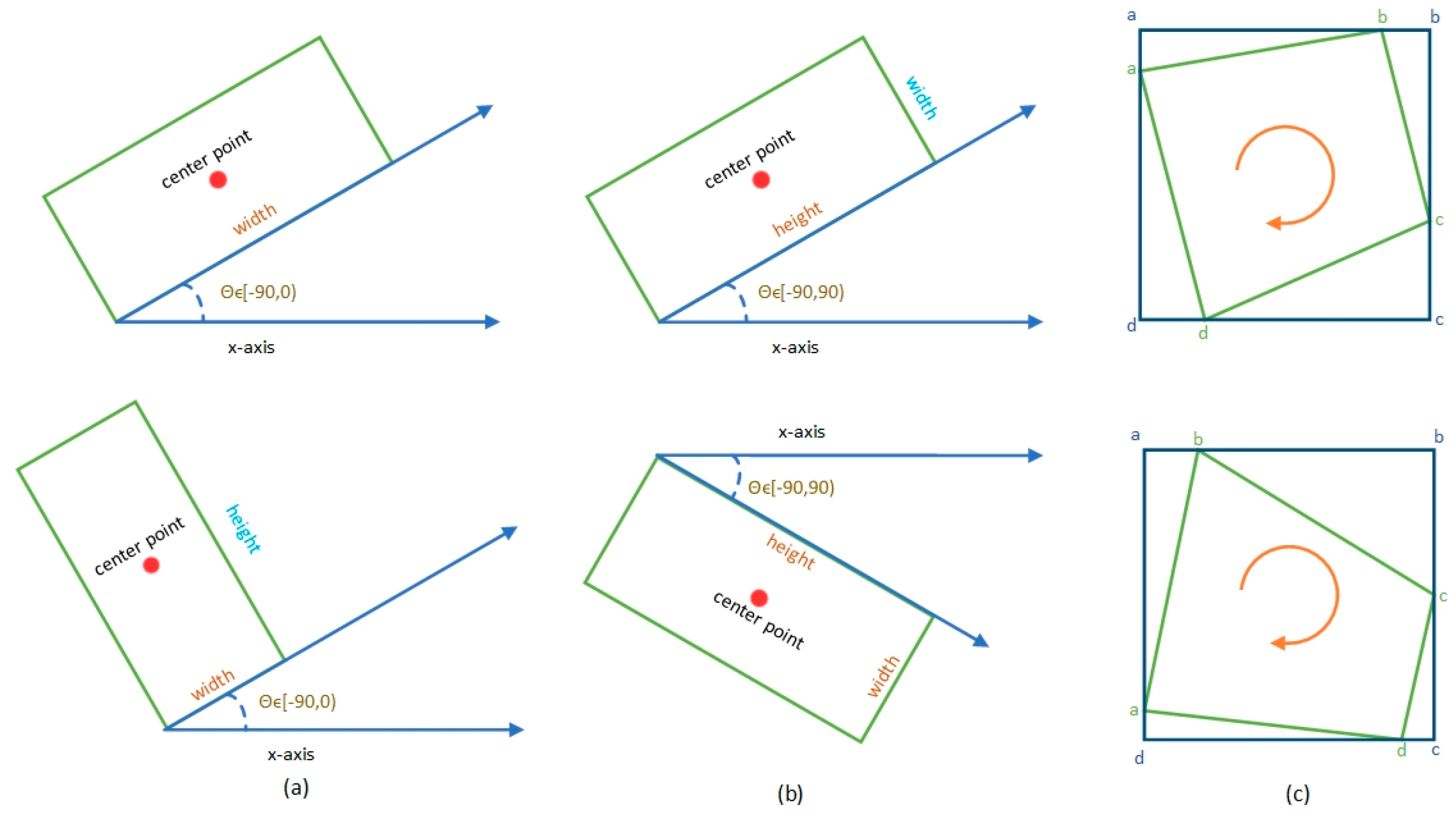
(2) The second challenge is the rotated bounding box. The orientation of the ship leads us to the need to predict angle information. There are three methods commonly used to define a rotated bounding box, namely the opencv definition method, the long-edge definition method and the ordered quadrilateral definition method. Figure 1 illustrates the definition details. The opencv method and the long-edge method are both five-parameter $(x,y,w,h,\theta )$ definition methods, where $(x,y)$ are the coordinates of the centre and $(w,h)$ are the length and width of the rotated bounding box. The difference is that the angle $\theta$ in the opencv method is the acute angle made by the box with the x-axis, and this side of the box is denoted as $w$, and the other side is denoted as $h$, so that the angle is expressed in the range $[-90, 0)$. The angle $\theta$ in the long-side method is the angle made by the long side $h$ of the box with the x-axis, so the angle is expressed in the range $[-90, 90)$. The ordered quadrilateral definition method $(x_1,y_1,x_2,y_2,x_3,y_3,x_4,y_4)$ takes the leftmost point as the starting point and orders the other points counterclockwise. The periodicity of angular (PoA) and the exchangeability of edges (EoE) can lead to angle predictions outside of our defined range. As a result, a large loss value is generated, triggering the boundary discontinuity problem, which affects training. These different methods share the same boundary problem. Since targets with large aspect ratios, such as ships, are very sensitive to changes in angle, it is of great interest to study the boundary problem. Figure 2 shows the boundary problem for the opencv method and the long-edge method. The ideal angle regression path in the opencv method is a counter-clockwise rotation from the blue box to the red box. However, there are two problems with PoA and EoE in the opencv-based approach due to the definition of $w,h ,$ and $\theta$. These two problems can lead to very high losses following this regression. Therefore, the model is only regressed in a clockwise direction. This regression method definitely increases the difficulty of the regression. The long-edge method can also be affected by PoA, resulting in a sudden increase in the loss value. To solve these problems, Yang et al. [24] proposed the Circular Label Smoothing (CSL) method, which turns angles into 180 categories for training. CSL was then further developed into the Densely Coded Label (DCL) method [25]. The DCL method mainly improves the number of prediction layers and the performance in square-like target detection. However, at the same time, the authors also point out that converting angles to classifications leads to an increase in theoretical errors and the number of model parameters. Subsequently, the Gaussian Wasserstein Distance (GWD) method was proposed by Yang et al. [26]. This method converts the rotating bounding box into a two-dimensional Gaussian distribution and uses the GWD to calculate the distance between the two Gaussian distributions. The authors use this distance value to reflect the similarity between two rotating bounding boxes, thus solving the problem of the Rotating Intersection-over-Unions (RIoU) not being differentiable. Yang et al. [26] proposed the use of Kullback–Leibler Divergence (KLD) instead of GWD to calculate the distance. Unlike Smooth L1 Loss and GWD Loss, KLD Loss is scale invariant and its center is not slightly displaced, allowing high-precision rotation detection. M. Llerena et al. [27] proposed a new loss function, the Probabilistic Intersection-over-Union (ProbIoU) loss function, which uses the Hellinger distance to measure the similarity of targets. Yang et al. [28] proposed the Kalman Filtering Intersection-over-Unions (KFIoU), which uses the idea of Gaussian multiplication to solve the problem of inconsistency between the metric and the loss function. Calculating the RIoU between two rotating bounding boxes has become the most important problem in rotation ship detection.

(3) The third challenge is that there are still few methods to solve the problem of simultaneous SAR ship detection and SAR ship classification. Zhang et al. [29] proposed a polarization fusion network with geometric feature embedding (PFGFE-Net) to alleviate the problem of polarization, insufficient utilization and traditional feature abandonment. Zhang et al. [30] proposed a multitask learning framework. The framework achieves better deep-feature extraction by integrating the dense convolutional networks. Zhang et al. [31] proposed a pyramid network with dual-polarization feature fusion for ship classification in SAR images. The network uses the attention mechanism to balance the features and performs dual-polarization feature fusion to effectively improve the ship classification performance. Zhang et al. [32] incorporated the traditional histogram of oriented gradient (HOG) feature into the ship classification network. The method fully exploits the potential of mature handcrafted features and global self-attention mechanisms, and achieves excellent results on the OpenSARShip dataset. All of these networks achieve the classification of SAR ships, but do not enable SAR ship detection. Part of the reason for this phenomenon is that SAR images contain a large amount of complex background information and multi-scale feature targets, making ship detection and classification extremely difficult. Another reason is the lack of a suitable dataset. Most of the existing research methods are based on ship detection datasets such as SSDD [33], AirSARship [34], HRSID [35] and LS-SSDD-v1.0 [36]. These datasets have limitations in terms of data quality and target labelling. The development of ship detection and classification is hampered by these conditions. Lei et al. [37] published a high-resolution SAR ship detection dataset (SRSDD). The dataset contains six categories of ships in complex scenarios and can be used for rotating target detection and category detection. Jiang et al. [38] proposed a feature extraction module, a feature context aggregation module, and a multi-scale feature fusion module. These modules improve the detection of small objects in complex backgrounds via the fusion of multi-scale features and contextual information mining, and have achieved good performance on the SRSDD. Zhang et al. [39] proposed a YOLOV5s-based ship detection method for SAR images. This network attempts to incorporate frequency domain information into the channel attention mechanism to improve the detection and classification performance. Shao et al. [40] proposed RBFA-Net for the rotational detection and classification of ships in SAR images. Although the above methods have made some progress in integrating ship detection and classification research, there is still room for improvement in terms of model performance and model size.

In order to address the above problems, a YOLOV8-based oriented ship detection and classification method for SAR images is proposed with lightweight receptor field feature convolution, bottleneck transformers and probabilistic intersection-over-union network (R-LRBPNet). The main objective of the network is to achieve the accurate detection and classification of ships while keeping the network lightweight. Firstly, our proposed C2fBT module is able to better extract integrated channel and global spatial features. Secondly, the R-LRBPNet presents an angle-decoupling module. In R-LRBPNet, the input feature maps are tuned for regression and classification tasks, respectively. The fast and accurate regression of angles is achieved using the ProbIoU + Distribution Focal Loss (DFL) [41] approach at the decoupling head. Finally, in the feature fusion stage, our proposed lightweight receptor field feature convolution (LRFConv) is used to improve the sensitivity of the network to multi-scale targets and its ability to discriminate between complex and detailed information, thus improving the network’s ability to classify ships.

The main contributions are as follows:

• A feature fusion module C2FBT is proposed. The module uses global spatial information to alleviate the problem of difficult detection due to the high density of ships. R-LRBPNet is proposed for SAR ship detection and classification.
• A separate angle-decoupling head and ProbIoU + DFL angle loss function are proposed. The model is effective in achieving accurate angle regression and reducing the imbalance between the angle regression task and other tasks.
• The LRFConv is proposed in R-LRBPNet. This module improves the network’s sensitivity to multi-scale targets and its ability to extract important detailed information.
• A large number of experiments on the SRSDD dataset show that our R-LRBPNet is able to accurately detect and classify ships compared to 13 other networks.

The remainder of this paper is organized as follows. In Section 2, we propose the overall framework of the model and introduce the methodology. The experiments are described in Section 3. In Section 4, we analyze the results of the comparison experiment and ablation experiment. Finally, Section 5 summarizes the paper.

2. Proposed Methods

2.1. Overview of the Proposed Model

2.1.1. Model Structure

The R-LRBPNet is designed on the basis of YOLOV8n. Its network structure is shown in Figure 3. The model structure is mainly divided into three parts: the backbone, neck and decoupling head.

• Backbone

The original backbone consisted of five convolutional modules, four C2f modules and a Spatial Pyramid Pooling—Fast (SPPF) module. The C2f block adopts a multi-gradient path strategy to diversify the depth of the model and improve its ability to perceive and learn from different features. In our network, in order to enhance the feature extraction capability of the backbone network, we have designed a new C2fBT module based on a transformer to replace the original C2f module. There have been relevant experiments proving [42] that the encoder part of the transformer only needs to handle high-level semantic features. The last layer of the backbone network has a feature map with a smaller size. Therefore, we add C2fBT to the last layer of the backbone. The following ablation experiments with C2fBT demonstrate that the module improves performance while reducing the number of model parameters.

• Neck

A path aggregation network (PAN) and feature pyramid network (FPN) constitute the neck. The original neck consists of four C2f modules, two convolutional modules, two upsampling and four Concat modules. The first C2f module in the neck is replaced with C2fBT and the first two convolution modules are replaced with our LRFConv. LRFConv is used to enhance the ability of the feature fusion phase network to extract the complex and detailed information contained in the feature maps and to adaptively extract the focal features of multi-scale targets. The reason for designing this structure will be given in the ablation experiments.

• Head

The R-LRBPNet proposes an angle prediction branch in order to solve the multi-angle problem of ship detection. Most current rotating frame detection models predict $(x,y,w,h,\theta )$ directly in a regression branch. There is experimental [43] evidence that the features required to predict $\theta$ are different from those required to predict $(x,y,w,h)$. Therefore, we design a decoupled angle prediction head to predict $\theta$. The decoupled head consists of two convolution layers and is very light. The structure of the decoupling head is shown in Figure 3.

2.1.2. Algorithmic Process

We first feed the image into the backbone network and extract the main features through the backbone network. The neck structure then uses the PAN to deliver the high-level semantic information to the low-level feature map and uses the FPN module to transfer the low-level feature information to the high-level feature map. The feature maps are then fed into the detection head to provide the required information for the different stages of the classification and regression tasks. Multi-task loss is calculated in the training phase. For angle branching, the loss is calculated using ProbIoU + DFL. During testing, non-maximization suppression (NMS) is used to build the detection predictions.

2.2. C2fBT

It is well known that the distribution of ships in SAR images is not regular, especially in in-shore contexts where ships are often densely arranged. In its high-level semantic feature map, some feature pixels represent ship location and category information, some represent important environmental information related to these ships, and some are irrelevant. The MHSA is a deep learning model based on a self-attention mechanism. It is able to automatically capture the dependencies between sequences when processing input sequences, leading to a better understanding of the contextual information and improved model performance. By applying MHSA to high-level semantic feature maps, the potential spatial relationships between different pixel features can be efficiently computed.

The self-attention mechanism is a core component of MHSA. The self-attention mechanism assigns weights to each element in an input sequence by computing the relevance of a query, key and value. Specifically, given an input sequence, it is mapped to the query, key and value vector space, then the associativity distribution is obtained by calculating the inner product of the query with all the keys, and then the associativity is multiplied and summed with the value vector to obtain the final self-attentive representation.

In order to improve the network’s spatial feature extraction capability in high-resolution SAR images of complex scenes, in this paper, a new global spatial information attention module (C2fBT) is designed; this is inspired by the C2f structure and MHSA in BotNet [BOT], and is obtained by integrating the MHSA into C2f. The C2fBT structure and the BoT structure are shown in Figure 4a and Figure 4b, respectively.

C2fBT is a hybrid model that uses convolution and MHSA. The structure computes queries $Q$, keys $K$, values $V$ and their positional parameters by three 1 × 1 convolutions. The formulae are as follows:

$$Q_h=X{W}_h^q,K_h=X{W}_h^k,V_h=X{W}_h^v$$

(1)

where $W_h^q,W_h^k,$ and $W_h^v$ are linear transformations of the input matrix $X$ to $Q,K,$ and $V$. The output of the head $O_h$ can be expressed as follows:

$$O_h=\mathrm{S}\mathrm{o}\mathrm{f}\mathrm{t}\mathrm{m}\mathrm{a}\mathrm{x}\left(\frac{Q_h{K}_h^T+S_h^H+S_h^W}{\sqrt{d_k^h}}\right)V_h,$$

(2)

where $S_h^H,S_h^W\in R^{HW\times HW}$ are the logarithmic matrices of the relative positions along the height and width dimensions, and $d_k^h$ is the dimension of keys in head h. The relative position matrix $S_h^H\left[i,j\right]$ and $S_h^W[i,j]$ are defined as follows:

$$S_h^H[i,j]=q_i^T{r}_{j_y-i_y}^H$$

(3)

$$S_h^W[i,j]=q_i^T{r}_{j_x-i_x}^W$$

(4)

where $q_i$ is the i-th row of queries Q, and $r_{j_y-i_y}^H$ and $q_i^T{r}_{j_x-i_x}^W$ are relative positional embeddings for height and width.

Overall, the C2fBT structure we have designed not only enriches the input information of the Concat operation, but also uses the global attention mechanism to process and aggregate the information contained in the convolutionally captured feature maps.

2.3. Decoupled Angle Prediction Head and ProbIoU Loss

There are relevant experiments [44] demonstrating the existence of an imbalance between the two tasks of classification and regression. However, we hypothesize that even in the same regression task, there is still a task imbalance. Therefore, to validate this hypothesis, this module designed two different regression branches to regress $(x,y,w,h)$ and $\theta$, respectively. The ablation experiments proved the effectiveness of the structure we designed.

The main difference between horizontal bounding box (HBB) and oriented bounding box (OBB) detection is that the computation of RIOU in OBB is not microscopic, resulting in the network not being trained. Therefore, achieving the accurate regression of the angle becomes the most important problem in rotation detection. The CSL and DCL method is widely used in current YOLO-based angle prediction methods due to its structural simplicity. However, the disadvantage of CSL and DCL is that it suffers from theoretical errors, as well as an increase in the number of model parameters and computational complexity. To address this current problem, ProbIoU is used to approximate the RioU between two rotated bounding boxes.

The Bhattacharyya Coefficient ($B_C$) is used in ProbIoU to calculate the degree of overlap between the Gaussian distributions of the two rotated bounding boxes, and the $B_C$ between the two probability density functions $p\left(x\right)$ and $q\left(x\right)$ is defined as follows:

$$B_C(p,q)={\int }_{{\mathbb{R}}^2}\sqrt{p\left(x\right)q\left(x\right)}dx$$

(5)

where $B_C\left(p,q\right)\in \left[0,1\right]$. This coefficient measures the degree of overlap between two distributions. The value of $B_C\left(p,q\right)$ is 1 only if the two distributions are identical. The Bhattacharyya distance ($B_D$) is defined to calculate the degree of similarity between two Gaussian distributions:

$$B_D\left(p,q\right)=-ln{B}_C\left(p,q\right)$$

(6)

Equation (6) provides an estimate of the similarity between $p,q$. $B_C$ and $B_D$ are inversely related. We assume that the Gaussian distributions of the two rotated bounding boxes are $p~\mathcal{N}\left({\mu }_1,{\mathsf{\Sigma }}_1\right), q~\mathcal{N}({\mu }_2,{\mathsf{\Sigma }}_2)$:

$${\mu }_1=\left(\genfrac{}{}{0pt}{}{x_1}{y_1}\right),{\mathsf{\Sigma }}_1=\left[\begin{array}{cc}{a}_1& c_1\\ c_1& b_1\end{array}\right], {\mu }_2=\left(\genfrac{}{}{0pt}{}{x_2}{y_2}\right),{\mathsf{\Sigma }}_2=\left[\begin{array}{cc}{a}_2& c_2\\ c_2& b_2\end{array}\right]$$

(7)

We can then obtain a closed-form expression for $B_D$ given by the following:

$$B_D=\frac{1}{8}({\mu }_1-{\mu }_2{)}^T{\mathsf{\Sigma }}^{-1}({\mu }_1-{\mu }_2)+\frac{1}{2}\mathrm{l}\mathrm{n}\left(\frac{det\mathsf{\Sigma }}{\sqrt{det{\mathsf{\Sigma }}_{1}det{\mathsf{\Sigma }}_2}}\right),\mathsf{\Sigma }=\frac{1}{2}\left({\mathsf{\Sigma }}_1+{\mathsf{\Sigma }}_2\right)$$

(8)

Then, ${\mu }_1$ and ${\mu }_2$ are brought into the above equation, and $B_D$ is disassembled to obtain $B_1$ and $B_2$:

$$B_1=\frac{1}{4}\frac{(a_1+a_2)(y_1-y_2{)}^2+(b_1+b_2\left)\right(x_1-x_2{)}^2+2(c_1+c_2)(x_2-x_1)(y_1-y_2)}{\left(a_1+a_2\right)\left(b_1+b_2\right)-(c_1+c_2{)}^2}$$

(9)

$$B_2=\frac{1}{2}\mathrm{l}\mathrm{n}\left(\frac{\left(a_1+a_2\right)\left(b_1+b_2\right)-(c_1+c_2{)}^2}{4\sqrt{(a_1{b}_1-c_1^2)(a_2{b}_2-c_2^2)}}\right)$$

(10)

where $B_D=B_1+B_2$, $B_C=e^{-B_D}$. $B_1$ and $B_2$ can be controlled by different hyperparameters to control their weight sizes. However, $B_D$ does not satisfy the triangle inequality, so it cannot be used to represent the true distance. The Hellinger distance has been used as an alternative to $B_D$ to compute the true distance metric:

$$H_D\left(p,q\right)=\sqrt{1-B_c\left(p,q\right)}$$

(11)

where $0\le H_D\left(p,q\right)\le 1$. This method allows the distance metric to be converted into a function of the Gaussian distribution parameters for ease of calculation. The Gaussian Bounding Boxes (GBBs) regressed by a network are defined as $p=\left({\mathrm{x}}_1,{\mathrm{y}}_1,{\mathrm{a}}_1,{\mathrm{b}}_1,{\mathrm{c}}_1\right)$ and the ground truth bounding box is defined as $q=\left({\mathrm{x}}_2,{\mathrm{y}}_2,{\mathrm{a}}_2,{\mathrm{b}}_2,{\mathrm{c}}_2\right)$. The loss function of ProbIoU should be as follows:

$${\mathcal{L}}_1\left(p,q\right)=H_D\left(p,q\right)=1-\mathrm{P}\mathrm{r}\mathrm{o}\mathrm{b}\mathrm{I}\mathrm{o}\mathrm{U}(p,q)\in [0,1]$$

(12)

$${\mathcal{L}}_2\left(p,q\right)=B_D\left(p,q\right)=-\mathrm{l}\mathrm{n}\left(1-{\mathcal{L}}_1^2(p,q)\right)\in [0,\mathrm{\infty }]$$

(13)

where a large distance between two Gaussian distributions in ${\mathcal{L}}_1\left(p,q\right)$ can lead to the problem of too-slow convergence during network training. ${\mathcal{L}}_2\left(p,q\right)$ is not a good representation of the relationship with the IoU. Therefore, our training pattern is to train first with ${\mathcal{L}}_2\left(p,q\right)$ and then with ${\mathcal{L}}_1\left(p,q\right)$ as the distance gets closer.

But there is another problem with using ProbIoU Loss as the regression loss. To compute ProbIoU Loss, the rotated bounding box is converted to a GBB. If the rotated bounding box is approximately square, the direction of the GBB is inherited from the ellipse, making it impossible to determine the direction of the rotating bounding box. The DFL Loss function is used to solve this problem. Specifically, the DFL discretizes the angle using a predetermined even interval $\delta$, which is subjected to an integration operation to obtain the predicted angle value $\theta$:

$$\theta ={\mathsf{\Sigma }}_{i=0}^{90}{p}_{i}i\delta$$

(14)

where $p_i$ denotes the probability of the angle falling in each interval.

2.4. Lightweight Receptive Field Feature Convolution

The LRFConv module is designed to improve the ability to extract detailed and complex information from SAR images. The module is designed based on RFAConv [45]. The distinguishing feature of traditional convolutional operations is the use of a convolutional kernel with shared parameters to extract features. Shared parameters cause the convolution to process each pixel equally, without taking into account the different importances of each pixel. We therefore replace some of the traditional convolution operations with LRFConv. This structure adjusts the weights of feature pixels within different sensory fields to highlight the details and complex information needed for important ship classification. The LRFConv structure is shown in Figure 5.

In LRFConv, the introduction of Receptive-Field Attention (RFA) allows the network to focus on the importance of features within different receptive fields and prioritize features in the receptive field space. The implementation of this attention mechanism is based on two main parts: the extraction of the receptive field space features and the generation of the attention graph. The first part concerns the generation of the attention map. The process is as follows: first, an average pooling operation is performed on the input feature map to preserve the global information in the feature map and to aggregate the information from all receptive fields. Second, a deep convolution [46] is performed on the feature map to facilitate the interaction of information within each receptive field. Then, the weights of each pixel feature within the receptive fields are adjusted using the SoftMax function to generate its corresponding attention weight map for each receptive field feature map. The second part is the generation of the receptive field spatial feature maps. The receptive field spatial feature is specifically designed for convolutional kernels and is dynamically generated based on the kernel size. The map is obtained by transforming the original feature map through non-overlapping sliding windows. Each sliding window represents a receptive field slider whose size can be dynamically adjusted according to the size of the convolutional kernel. In this way, the network is able to generate receptive field spatial features of the appropriate size according to the size of the convolution kernel. We obtain the receptive field spatial feature map by performing a series of 3 × 3 convolution operations on the input feature map. Finally, the feature maps with rich receptive field information are fused with the obtained weighted feature maps. Different weights are assigned to each receptive field location and feature channel using the receptive field weight matrix to highlight important detailed features. And the size of the output feature map is adjusted to obtain the final output.

In LRFConv, the introduction of Receptive-Field Attention (RFA) allows the network to focus on the importance of features within different receptive fields and prioritize features in the receptive field space. The implementation of this attention mechanism is based on two main parts: the extraction of the receptive field space features and the generation of the attention graph. The first part concerns the generation of the attention map. The process is as follows: first, an average pooling operation is performed on the input feature map to preserve the global information in the feature map and to aggregate the information from all receptive fields. Second, a deep convolution [46] is performed on the feature map to facilitate the interaction of information within each receptive field. Then, the weights of each pixel feature within the receptive fields are adjusted using the SoftMax function to generate its corresponding attention weight map for each receptive field feature map. The second part is the generation of the receptive field spatial feature maps. The receptive field spatial feature is specifically designed for convolutional kernels and is dynamically generated based on the kernel size. The map is obtained by transforming the original feature map through non-overlapping sliding windows. Each sliding window represents a receptive field slider whose size can be dynamically adjusted according to the size of the convolutional kernel. In this way, the network is able to generate receptive field spatial features of the appropriate size according to the size of the convolution kernel. We obtain the receptive field spatial feature map by performing a series of 3 × 3 convolution operations on the input feature map. Finally, the feature maps with rich receptive field information are fused with the obtained weighted feature maps. Different weights are assigned to each receptive field location and feature channel using the receptive field weight matrix to highlight important detailed features. And the size of the output feature map is adjusted to obtain the final output.

The LRFConv calculation can be expressed as follows:

$$F=Softmax\left({DW}^{1\times 1}\left(AvgPool\left(f_x\right)\right)\right)\times ReLU\left(Norm\left(g^{k\times k}\left(f_x\right)\right)\right)=A_{rf}\times F_{rf}$$

(15)

where $g^{x\times x}$ represents a grouping convolution of size $x\times x$, $DW$ represents the DWConv, $k$ represents the convolution kernel size, $f_x$ represents the input feature map, $A_{rf}$ represents the pixel feature weight map, $F_{rf}$ represents a map of spatial features in the receptive field and $F$ represents the final output.

Overall, our LRFconv has two advantages. First, it can dynamically adjust the size of the receptive field according to the size of the convolutional kernel and generate the corresponding spatial feature maps of the receptive field. For example, a large receptive field is generated for large ships such as cargo ships and oil tankers to capture global features, and a small receptive field is generated for small-scale fishing ships to capture local detail information. Second, it can assign different weights to each receptive field location and feature channel, and use this method to obtain the required detailed features. These advantages can help our network to achieve accurate ship classification.

3. Experiments

3.1. Datasets

We chose to perform our ship detection and classification experiments on the SRSDD-v1.0 dataset. All raw SAR images in this dataset are from the GF-3 satellite at 1 m resolution in SL mode, and the original 30 panoramic images are cropped to 666 images containing 2884 ships at 1024 × 1024, with rotated bounding box labels. In the SRSDD, in-shore scenes accounted for 63.1% and off-shore scenes accounted for 36.9%. The number of images containing land was 420, including 2275 ships. The number of images containing only sea is 246, with 609 ships. In total, the dataset contains six different categories, including container ships, fishing ships, bulk cargo ships (cell-container ships), ore–oil ships, dredger ships and law enforcement ships. The dataset also suffers from certain category imbalance problems, which can lead to higher requirements for the detection algorithms. The exact distribution of the data is shown in Figure 6 and Figure 7.

The SSDD+ dataset is composed of 1160 SAR images containing 2456 ship targets, all of which are rotationally labelled in the SSDD+ dataset. The images are derived from multi-scale ship slices from the RADARSAT-2, TerraSAR-X and Sentinel-1 satellites, with image resolutions ranging from 1 m to 15 m. The SSDD+ dataset is divided into training and validation sets according to an 8:2 ratio. We chose the SSDD+ dataset to verify the generalization of R-LRBPNet.

3.2. Experimental Details

The experimental environment was the pytorch 1.8.0 deep learning framework based on python3.9, the test and validation environment was the ubuntu18.04 system, and the model performance evaluation was performed on 8 GB NVIDIA GeForce RTX 3070 GPUs with CUDA11.4 and CUDNN accelerated training. To ensure the fairness of the experiments, the comparison experiments were performed using the MMRotate [47] toolbox.

In this paper, the stochastic gradient descent (SGD) optimizer is used for training. The image input size is set to 1024 × 1024 for the SRSDD dataset and 512 × 512 for the SSDD+ dataset. The network has the same parameters except for the input image resolution. The network batch size is 8, the epoch is 500, the learning rate is 0.01, and the momentum and weight decay rates are 0.0005 and 0.8, respectively. The detection IOU threshold is set to 0.5 for the test, and all other parameters are adopted as default.

3.3. Evaluation Metrics

To validate the model performance, we used Precision, Recall, the mean average precision (mAP), $F1score$ and model size as evaluation metrics to evaluate different models in our experiments. The Recall, Precision and average precision are defined as follows:

$$\mathit{Precision}=\frac{TP}{TP+FP}$$

(16)

$$\mathit{Re}call=\frac{TP}{TP+FN}$$

(17)

$$AP={\int }_0^{1}P\left(R\right)\mathrm{d}R$$

(18)

$$mAP=\frac{1}{k}\sum _{i=1}^{k}A{P}_i$$

(19)

where $TP$ stands for true positives and indicates the number of samples correctly classified as positive samples, $TP$ stands for false positives and indicates the number of samples incorrectly classified as positive samples, $FN$ stands for false negatives and indicates the number of samples incorrectly classified as negative samples and $P\left(R\right)$ is the precision–recall curve. Precision and recall are both reflected in the F1score, with the following equation:

$$F1score=2\times \frac{Precision\times Recall}{Precision+Recall}$$

(20)

Finally, the model size is used to measure the complexity of the algorithm.

4. Results

4.1. Ablation Studies

In this section, we present the results of the ablation experiments carried out on SRSDD-v1.0 and evaluate our improvement.

4.1.1. Effect of C2fBT

Table 1. Detection results of different transformer modules on SRSDD-v1.0.

Module	Precision (%)	Recall (%)	F1Score	mAP (%)	FPS	Module Size (M)
C2f	72.1	56.7	63.47	65.2	140.8	7.1
C2F+VisionTrans	67.6	66.2	66.89	68.7	129.4	7.0
C3+VisionTrans	69.6	53.2	60.30	67.3	138.3	6.8
C2fBT	73.5	57.6	64.59	69.3	113.6	6.5

and

Table 2. Ship detection results of the AP of each category with different transformer modules.

Module	Ore-Oil	Cell-Container	Fishing	Law Enforce	Dredger	Container
C2f	47.9	78.8	43.1	93.8	82.4	56.8
C2F+VisionTrans	60.4	69.0	52.3	83.9	84.4	61.5
C3+VisionTrans	51.0	81.2	38.0	89.8	84.9	59.2
C2fBT	46.7	74.0	48.3	99.5	88.7	58.8

show the ablation study results on C2fBT. We designed four structures for comparison, namely a Vision Transformer [48] integrated on C2f, a Bottleneck Transformer integrated on C2f, and a Vision Transformer integrated on cross-stage partial bottleneck-based YOLOV5 and C2f. We replaced the last C2f module in the backbone network with each of the above modules. Except for the C2f part, the networks used in the experiment were exactly the same. It can be seen that there are some performance improvements in several of the above improvements. Among them, the performance of the C2fBT we designed shows greater improvement in identifying fishing ships, law enforcement ships, and dredger ships, especially law enforcement ships. This is due to the fact that bulk cargo ships, fishing ships and law enforcement ships are mostly distributed along the coastline, with small and densely distributed targets, which poses certain challenges for ship detection and classification. Our designed C2fBT can effectively capture the global spatial information of the distribution of ships, and can effectively identify such densely arranged difficult targets. The C2fBT achieves 4.1%, 1.4%, 0.9% and 1.12 improvements in the mAP, precision, recall and F1 score, respectively, and also reduces the size of module by 0.6 M. However, it should also be noted that as the complexity of the C2f module increases, the FPS (frames per second) of the model decreases. The FPS can be used as one of the indicators to measure the inference speed of the model. As shown in the table, the FPS of the C2fBT module decreased from 140.8 to 113.6 compared to the original C2f module. Overall, our C2fBT achieves a higher model performance at the cost of moderate FPS losses.

In the following visualization results, the white rectangular box represents a miscarriage of justice, the white circular box represents a misdetection, the white elliptical box represents a missed detection, yellow represents ore–oil ships, orange represents cell–container ships, pink represents fishing ships, green represents law enforcement ships, brown represents dredger ships, and red represents container ships. From the comparison of the visualization results in Figure 8, we can find that the C2fBT can accurately detect densely packed ships and achieve accurate category classification for ships whose categories are easily confused in some in-shore scenarios.

4.1.2. Effect of Decoupled Head and ProbIoU Loss

In this section, we perform comparative experiments using CSL based on angle classification methods, KLD and KFIoU based on angular regression methods, and ProbIoU methods that do not use angle decoupling. As can be seen in

Table 3. Detection results of different angle regression methods on SRSDD-v1.0.

Module	Precision (%)	Recall (%)	mAP (%)
CSL	64.2	46.5	46.6
KLD	74.4	63.9	69.7
KFIoU	76.2	64.1	70.7
ProbIoU	76.8	64.9	71.0
ProbIoU+ angle decoupling+ DFL	78.2	64.2	71.8

, the CSL that converts angle predictions to classification problems performs the worst. The angle regression method of modelling the rotating bounding box as a Gaussian distribution performed better overall. Our proposed ProbIoU module performs well in all evaluation metrics. This indicates that ProbIoU+ angle decoupling+ DFL is more suitable for our model structure.

4.1.3. Effect of LRFConv

In this section, we will focus on the comparison between the LRFConv module and the CBAM [49] module, as well as the comparison between our LRFConv+ C2fBT module at different locations in the network. The ablation experiments are shown in

Table 4. Detection validity of LRFConv on SRSDD-v1.0.

Module	Precision (%)	Recall (%)	F1score	mAP (%)	Module Size (M)
LRFConv	66.1	57.7	61.62	63.8	7.0
CBAM	67.7	55.4	60.93	62.5	7.0
LRFConv+ C2fBT (1)	78.2	64.2	70.51	71.8	6.8
LRFConv+ C2fBT (2)	73.5	62.1	67.32	68.5	7.3
LRFConv+ C2fBT (3)	79.9	56.5	66.19	70.8	7.5

and

Table 5. Ship detection results of the AP of each category for several models.

Module	Ore-Oil	Cell-Container	Fishing	Law Enforce	Dredger	Container
LRFConv	52.5	69.4	37.9	87.9	80.3	54.7
CBAM	49.9	72.7	33.0	87.9	80.0	51.6
LRFConv+ C2fBT (1)	52	77.3	54.5	99.5	82.6	60.7
LRFConv+ C2fBT (2)	54.7	76.2	48.4	90	82.2	59.8
LRFConv+ C2fBT (3)	59.5	81.0	42.4	99.5	82.8	59.4

.

From the results in the table, it can be seen that although both CBAM and LRFConv are spatial attention mechanisms, our LRFConv is able to improve the mAP by 1.3% while maintaining its light weight. This is because LRFConv can dynamically adjust the receptive field to the target scale to capture critical information and complex details. As a result, the LRFConv module is well suited to the recognition and detection of difficult multi-scale samples with similar features.

In addition, we have investigated the correct location of the LRFConv and C2fBT module in the network through ablation experiments. The positional design of the LRFConv refers to the positional design of the spatial attention, while the positional design of the C2fBT module refers to the positional design of the transformers. LRFConv+ C2fBT (1) represents replacing C2f with our C2fBT only in the last layer of the backbone network and adding two LRFConv layers in the neck network. The purpose of such a structure is to reduce the computational cost while maximizing the extraction of global spatial and detail information from the feature map. LRFConv+ C2fBT (2) is based on LRFConv+ C2fBT (1) by adding the LRFConv layer in front of the three detection heads. LRFConv+ C2fBT (3) replaces the convolution module of the neck network with LRFConv on top of LRFConv+ C2fBT (1), which is based on the idea of further extracting the spatial feature information on the high-level semantic map.

Figure 9 shows the results of the visualization of these five different structures on the SRSDD dataset. We can find that as the number of layers in the network increases, the classification rate of the network increases linearly for ore–oil ships, bulk cargo ships and fishing ships. Our LRFConv+ C2fBT module is able to efficiently extract the detail information in the images, leading to a gradual increase in the recognition rate in the network for ore–oil ships, which have a high overlap with coastal features, and for small ships with similar characteristics, such as fishing ships and bulk cargo ships. However, for large ships such as dredger ships and container ships, the detection rate decreases, the model recall and mAP decrease, and the model parameters increase. We therefore use the lightest structure, LRFConv+ C2fBT (1), which also has the best overall evaluation metrics. This structure improves precision by 2.1%, recall by 7.5%, mAP by 8%, F1 score by 8.89 and the number of parameters by 0.2 M compared to LRFConv.

4.2. Comparison with Other Methods

In order to verify the overall performance of the proposed network, we have selected some current mainstream single-stage and two-stage rotation detection algorithms, such as O-RCNN, ROI, R-Retina Net and R3Det, and 13 other models for comparative tests. The results are shown in

Table 6. Detection results of different CNN-based methods on SRSDD-v1.0.

Module	Precision (%)	Recall (%)	F1Score	mAP (%)	Module Size (M)
FR-O [50]	49.66	57.12	53.13	53.93	315
ROI [51]	51.22	59.31	54.97	54.38	421
Gliding Vertex [52]	53.95	57.75	55.79	55.79	315
O-RCNN [53]	64.01	57.61	60.64	56.23	315
R-Retina Net [13]	12.55	53.52	20.33	32.73	277
R3Det [54]	15.41	58.06	24.36	39.12	468
BBAVectors [55]	34.56	50.08	40.90	45.33	829
R-FCOS [56]	18.42	60.56	28.25	49.49	244
RTMDet [57]	-	-	-	56.00	-
RBFA-Net [40]	-	-	-	63.42	-
MFCANet [58]	-	-	-	66.28	-
R-YOLOV5 [39]	59.70	62.90	61.26	-	4.52
R-YOLOV8 [59]	73.50	56.70	64.01	65.21	7.11
R-LRBPNet	78.20	64.20	70.51	71.85	6.83

and

Table 7. Ship detection results of the AP of each category with different CNN-based methods.

Module	Ore-Oil	Cell-Container	Fishing	Law Enforce	Dredger	Container
FR-O	55.6	46.7	30.8	27.2	77.8	85.3
ROI	61.4	48.8	32.8	27.2	79.4	76.4
Gliding Vertex	43.4	52.8	34.6	28.2	71.2	79.6
O-RCNN	63.5	57.5	35.3	27.2	77.5	76.1
R-Retina Net	30.3	35.7	11.4	2.1	67.7	48.9
R3Det	44.6	42.9	18.3	1.1	54.3	73.5
BBAVectors	54.3	34.8	21.0	1.1	82.2	78.5
R-FCOS	54.8	47.3	25.1	5.4	83.0	81.1
RTMDet	59.4	76.5	40.0	27.3	80.5	52.3
RBFA-Net	59.4	57.4	41.5	73.5	77.2	71.6
MFCANet	66.2	73.0	31.4	94.8	81.8	50.5
R-YOLOV8	47.9	78.8	43.1	93.8	82.4	56.8
R-LRBPNet	54.0	77.3	54.5	99.5	82.6	63.2

.

The upper part of the table represents the two-stage model and the lower part the one-stage model. Table 6 shows that the two-stage detection method is more consistent. Among the two-stage detection models, O-RCNN has the best detection performance on the SRSDD dataset, with the highest precision, F1score and mAP. The reason for this is that the SRSDD dataset contains many images with complex background clutter, which is not conducive to algorithmic detection. The two-stage detection algorithm mitigates this type of problem by performing some initial filtering in the first stage.

Among the one-stage detection models, our proposed R-LRBPNet and anchor-free R-YOLOV8 are at the highest level in terms of precision, recall, F1 score, mAP and module size. The precision of R-LRBPNet has risen by 4.7% compared to R-yolov8n, which has the highest precision, the recall has risen by 3.64% compared to R-FCOS, which has the highest recall, the F1 scores have risen by 6.5% compared to R-YOLOV8, which has the highest F1 scores, and mAP has risen by 5.57% compared to MFCANet, which has the highest mAP. More importantly, the size of our R-LRBPNet model is drastically reduced compared to mainstream models, with a model size of only 6.8 M.

Table 7 shows that R-LRBPNet performs particularly well in the detection of fishing ships and law enforcement ships, with APs of 54.5% and 99.5% respectively. Cell–container ships have an AP of 77.3%, only slightly lower than R-YOLOv8. R-LRBPNet also achieves a high AP of 82.6% for the detection of dredgers, which is only second to that of R-FCOS. In addition, R-LRBPNet achieves APs of 54.0% and 63.2% for the detection of ore–oil ships and container ships, which are equally good in terms of detection performance for these two categories when compared to the other 13 detection methods. Overall, R-LRBPNet shows a balanced and excellent detection performance in all categories of ships and is undoubtedly the best choice.

Figure 10 illustrates the Precision–Recall Curve (PRC) and the confusion matrix of R-LRBPNet. The confusion matrix can effectively show the accuracy of the network’s classification of ships, where the horizontal coordinate is the actual category and the vertical coordinate is the predicted category. The diagonal line represents the probability of correct classification and the others the probability of misclassification. It can be seen that the network achieves the best detection performance for law enforcement ships, with little misclassification. Container ships, cell–container ships and dredger ships are also detected with relatively high accuracy, with an accuracy only slightly lower than that for law enforcement ships. There are more cases of misclassification for fishing ships compared to the other categories. It can be seen that the model easily identifies fishing ships as container ships or background true negatives, although the R-LRBPNet achieves an AP value of 54.5% for fishing ships, which is the highest value of all compared methods. Compared to recent rotating ship detection and classification methods [41,42,59] based on the SRSDD dataset, R-LRBPNet shows better performance. This is reflected not only in quantitative metrics such as detection accuracy and recall, but also in its ability to accurately detect different classifications of ship targets.

In

Table 8. Detection results of different CNN-based methods on SSDD+.

	Module	Precision (%)	Recall (%)	mAP (%)
Two stage	ReDet [60]	89.36	92.09	88.65
	ROI	90.05	91.31	89.04
	Gliding Vertex	88.00	89.62	87.97
	O-RCNN	85.64	88.12	84.65
One stage	R-Retina Net	76.18	76.53	70.83
	R3Det	85.22	86.00	82.72
	S2Anet [61]	90.38	91.09	88.36
	KLD	91.57	91.63	89.10
	KFIoU	91.68	93.12	90.25
	R-LRBPNet	94.77	94.09	91.67

, all algorithms except R-LRBPNet use ResNet50 as the feature extraction network. The table shows the performance of some classical one-stage and two-stage algorithms on the SSDD+ dataset. Similar to Table 6, the two-stage algorithms have the same stable performance on the SSDD+ dataset. The ROI method has the highest mAP of 89.04%. The precision, recall and mAP values of R-LRBPNet are 94.77%, 94.09% and 91.67%, respectively. The experimental results of R-LRBPNet on the SSDD+ dataset prove that the performance of R-LRBPNet on the other SAR datasets also has excellent robustness.

4.3. Detection and Classification Results on SRSDD

Figure 11 and Figure 12 show the visualization results of partial detection and classification for the different models on the SRSDD dataset for both the in-shore and off-shore scenes.

As we can see from Figure 11 and Figure 12, R-LRBPNet basically detects ships near the shore. This is because R-LRBPNet uses C2fBT and LRFConv to extract rich global spatial information and detail information, which reduces the negative impact of background interference. Therefore, even for small ships and densely clustered ships close to the shore, our network can accurately detect them.

Second, R-LRBPNet achieves accurate angle predictions in both in-shore and off-shore scenarios. This is because our angle-decoupling header can provide more appropriate feature maps for angle regression and because ProbIoU + DFL can provide more accurate losses for angle regression. Finally, our network achieves accurate classification even for difficult samples. For example, the features of fishing ships and bulk cargo ships in an SAR image are similar, and both are small targets. R-LRBPNet uses LRFConv to dynamically adjust the receptive field according to the size of the target, preserving key details. In addition, the decoupling module of the network also adaptively enhances the feature map. As a result, our network is able to correctly classify fishing ships and bulk cargo ships.

5. Conclusions

In this paper, a new lightweight method entitled R-LRBPNet is proposed for simultaneous directional ship classification and detection in SAR images. The network first extracts global spatial features for the detection of densely arranged ships using the modified feature extraction module C2fBT. Second, the network proposes an angle-decoupling head to alleviate the problem of imbalance between angle regression and other tasks. The ProbIoU and DFL methods are used in the decoupling head to compute the loss of the rotated bounding box and achieve accurate angle regression. Finally, LRFConv is used to increase the sensitivity of the network to details and important information in the feature map to achieve accurate ship classification. We conducted a series of comparison and ablation experiments on the SRSDD dataset to demonstrate the ship detection and classification performance of the network. The experimental results show that our network achieves the best performance compared to 13 other methods based on the SRSDD dataset. Also, the experimental results of the model on SSDD+ verify that the model has strong generalization. Our models have also been lightweighted, reducing their size to 6.8 M while maintaining performance.

However, our model also has shortcomings. For example, the angle prediction accuracy of the network still needs to be improved. The transformer structure in C2fBT reduces the model parameters and model size, but at the same time, it inevitably increases the model complexity and training time. The training of the baseline model YOLOv8 took longer, so the introduction of C2fBT would increase the training time of R-LRBPNet. Therefore, our next work will mainly focus on the following aspects: (1) The optimization of the model architecture to reduce time costs. (2) Investigating more suitable loss functions for angle regression. (3) Building a ship detection and recognition dataset with more categories and numbers. (4) Investigating how to quickly perform ship detection and classification in SAR images.

References

1. Zhang, C.; Gao, G.; Liu, J.; Duan, D. Oriented Ship Detection Based on Soft Thresholding and Context Information in SAR Images of Complex Scenes. IEEE Trans. Geosci. Remote Sens. 2024, 62, 5200615. [Google Scholar] [CrossRef]
2. Gao, G.; Zhang, C.; Zhang, L.; Duan, D. Scattering Characteristic-Aware Fully Polarized SAR Ship Detection Network Based on a Four-Component Decomposition Model. IEEE Trans. Geosci. Remote Sens. 2023, 61, 5222722. [Google Scholar] [CrossRef]
3. Liu, T.; Zhang, J.; Gao, G.; Yang, J.; Marino, A. CFAR ship detection in polarimetric synthetic aperture radar images based on whitening filter. IEEE Trans. Geosci. Remote Sens. 2019, 58, 58–81. [Google Scholar] [CrossRef]
4. Huang, X.; Yang, W.; Zhang, H.; Xia, G.-S. Automatic ship detection in SAR images using multi-scale heterogeneities and an a contrario decision. Remote Sens. 2015, 7, 7695–7711. [Google Scholar] [CrossRef]
5. Schwegmann, C.P.; Kleynhans, W.; Salmon, B.P. Synthetic aperture radar ship detection using Haar-like features. IEEE Geosci. Remote Sens. Lett. 2016, 14, 154–158. [Google Scholar] [CrossRef]
6. Redmon, J.; Divvala, S.; Girshick, R.; Farhadi, A. You only look once: Unified, real-time object detection. In Proceedings of the IEEE Conference on Computer Vision and Pattern Recognition, Las Vegas, NV, USA, 27–30 June 2016; pp. 779–788. [Google Scholar]
7. Zhang, T.; Zhang, X.; Shi, J.; Wei, S. Depthwise separable convolution neural network for high-speed SAR ship detection. Remote Sens. 2019, 11, 2483. [Google Scholar] [CrossRef]
8. Wang, J.; Lin, Y.; Guo, J.; Zhuang, L. SSS-YOLO: Towards more accurate detection for small ships in SAR image. Remote Sens. Lett. 2021, 12, 93–102. [Google Scholar] [CrossRef]
9. Liu, W.; Anguelov, D.; Erhan, D.; Szegedy, C.; Reed, S.; Fu, C.-Y.; Berg, A.C. Ssd: Single shot multibox detector. In Proceedings of the Computer Vision–ECCV 2016: 14th European Conference, Amsterdam, The Netherlands, 11–14 October 2016; pp. 21–37. [Google Scholar]
10. Zhang, T.; Zhang, X. High-speed ship detection in SAR images based on a grid convolutional neural network. Remote Sens. 2019, 11, 1206. [Google Scholar] [CrossRef]
11. Redmon, J.; Farhadi, A. YOLO9000: Better, faster, stronger. In Proceedings of the IEEE Conference on Computer Vision and Pattern Recognition, Honolulu, HI, USA, 21–26 July 2017; pp. 7263–7271. [Google Scholar]
12. Zhang, T.; Zhang, X. ShipDeNet-20: An only 20 convolution layers and <1-MB lightweight SAR ship detector. IEEE Geosci. Remote Sens. Lett. 2020, 18, 1234–1238. [Google Scholar]
13. Lin, T.-Y.; Goyal, P.; Girshick, R.; He, K.; Dollár, P. Focal loss for dense object detection. In Proceedings of the IEEE International Conference on Computer Vision, Venice, Italy, 22–29 October 2017; pp. 2980–2988. [Google Scholar]
14. Sun, Z.; Leng, X.; Lei, Y.; Xiong, B.; Ji, K.; Kuang, G. BiFA-YOLO: A novel YOLO-based method for arbitrary-oriented ship detection in high-resolution SAR images. Remote Sens. 2021, 13, 4209. [Google Scholar] [CrossRef]
15. Zhu, H.; Xie, Y.; Huang, H.; Jing, C.; Rong, Y.; Wang, C. DB-YOLO: A duplicate bilateral YOLO network for multi-scale ship detection in SAR images. Sensors 2021, 21, 8146. [Google Scholar] [CrossRef]
16. Guo, Q.; Liu, J.; Kaliuzhnyi, M. YOLOX-SAR: High-precision object detection system based on visible and infrared sensors for SAR remote sensing. IEEE Sens. J. 2022, 22, 17243–17253. [Google Scholar] [CrossRef]
17. Vaswani, A.; Shazeer, N.; Parmar, N.; Uszkoreit, J.; Jones, L.; Gomez, A.N.; Kaiser, Ł.; Polosukhin, I. Attention is all you need. Adv. Neural Inf. Process. Syst. 2017, 30. [Google Scholar] [CrossRef]
18. Naseer, M.M.; Ranasinghe, K.; Khan, S.H.; Hayat, M.; Shahbaz Khan, F.; Yang, M.-H. Intriguing properties of vision transformers. Adv. Neural Inf. Process. Syst. 2021, 34, 23296–23308. [Google Scholar]
19. Zhu, X.; Lyu, S.; Wang, X.; Zhao, Q. TPH-YOLOv5: Improved YOLOv5 based on transformer prediction head for object detection on drone-captured scenarios. In Proceedings of the IEEE/CVF International Conference on Computer Vision, Montreal, BC, Canada, 11–17 October 2021; pp. 2778–2788. [Google Scholar]
20. Li, Y.; Yao, T.; Pan, Y.; Mei, T. Contextual transformer networks for visual recognition. IEEE Trans. Pattern Anal. Mach. Intell. 2022, 45, 1489–1500. [Google Scholar] [CrossRef] [PubMed]
21. Srinivas, A.; Lin, T.-Y.; Parmar, N.; Shlens, J.; Abbeel, P.; Vaswani, A. Bottleneck transformers for visual recognition. In Proceedings of the IEEE/CVF Conference on Computer Vision and Pattern Recognition, Nashville, TN, USA, 20–25 June 2021; pp. 16519–16529. [Google Scholar]
22. Feng, J.; Wang, J.; Qin, R. Lightweight detection network for arbitrary-oriented vehicles in UAV imagery via precise positional information encoding and bidirectional feature fusion. Int. J. Remote Sens. 2023, 44, 4529–4558. [Google Scholar] [CrossRef]
23. Yu, Y.; Zhao, J.; Gong, Q.; Huang, C.; Zheng, G.; Ma, J. Real-time underwater maritime object detection in side-scan sonar images based on transformer-YOLOv5. Remote Sens. 2021, 13, 3555. [Google Scholar] [CrossRef]
24. Yang, X.; Yan, J. Arbitrary-oriented object detection with circular smooth label. In Proceedings of the Computer Vision–ECCV 2020: 16th European Conference, Glasgow, UK, 23–28 August 2020; pp. 677–694. [Google Scholar]
25. Yang, X.; Hou, L.; Zhou, Y.; Wang, W.; Yan, J. Dense label encoding for boundary discontinuity free rotation detection. In Proceedings of the IEEE/CVF Conference on Computer Vision and Pattern Recognition, Nashville, TN, USA, 20–25 June 2021; pp. 15819–15829. [Google Scholar]
26. Yang, X.; Zhang, G.; Yang, X.; Zhou, Y.; Wang, W.; Tang, J.; He, T.; Yan, J. Detecting rotated objects as gaussian distributions and its 3-d generalization. IEEE Trans. Pattern Anal. Mach. Intell. 2022, 45, 4335–4354. [Google Scholar] [CrossRef]
27. Llerena, J.M.; Zeni, L.F.; Kristen, L.N.; Jung, C. Gaussian bounding boxes and probabilistic intersection-over-union for object detection. arXiv 2021, arXiv:2106.06072. [Google Scholar]
28. Yang, X.; Zhou, Y.; Zhang, G.; Yang, J.; Wang, W.; Yan, J.; Zhang, X.; Tian, Q. The KFIoU loss for rotated object detection. arXiv 2022, arXiv:2201.12558. [Google Scholar]
29. Zhang, T.; Zhang, X. A polarization fusion network with geometric feature embedding for SAR ship classification. Pattern Recognit. 2022, 123, 108365. [Google Scholar] [CrossRef]
30. He, J.; Wang, Y.; Liu, H. Ship classification in medium-resolution SAR images via densely connected triplet CNNs integrating Fisher discrimination regularized metric learning. IEEE Trans. Geosci. Remote Sens. 2020, 59, 3022–3039. [Google Scholar] [CrossRef]
31. Zhang, T.; Zhang, X. Squeeze-and-excitation Laplacian pyramid network with dual-polarization feature fusion for ship classification in SAR images. IEEE Geosci. Remote Sens. Lett. 2021, 19, 4019905. [Google Scholar] [CrossRef]
32. Zeng, L.; Zhu, Q.; Lu, D.; Zhang, T.; Wang, H.; Yin, J.; Yang, J. Dual-polarized SAR ship grained classification based on CNN with hybrid channel feature loss. IEEE Geosci. Remote Sens. Lett. 2021, 19, 4011905. [Google Scholar] [CrossRef]
33. Zhang, T.; Zhang, X.; Li, J.; Xu, X.; Wang, B.; Zhan, X.; Xu, Y.; Ke, X.; Zeng, T.; Su, H. SAR ship detection dataset (SSDD): Official release and comprehensive data analysis. Remote Sens. 2021, 13, 3690. [Google Scholar] [CrossRef]
34. Xian, S.; Zhirui, W.; Yuanrui, S.; Wenhui, D.; Yue, Z.; Kun, F. AIR-SARShip-1.0: High-resolution SAR ship detection dataset. J. Radars 2019, 8, 852–863. [Google Scholar]
35. Wei, S.; Zeng, X.; Qu, Q.; Wang, M.; Su, H.; Shi, J. HRSID: A high-resolution SAR images dataset for ship detection and instance segmentation. IEEE Access 2020, 8, 120234–120254. [Google Scholar] [CrossRef]
36. Zhang, T.; Zhang, X.; Ke, X.; Zhan, X.; Shi, J.; Wei, S.; Pan, D.; Li, J.; Su, H.; Zhou, Y. LS-SSDD-v1.0: A deep learning dataset dedicated to small ship detection from large-scale Sentinel-1 SAR images. Remote Sens. 2020, 12, 2997. [Google Scholar] [CrossRef]
37. Lei, S.; Lu, D.; Qiu, X.; Ding, C. SRSDD-v1.0: A high-resolution SAR rotation ship detection dataset. Remote Sens. 2021, 13, 5104. [Google Scholar] [CrossRef]
38. Jiang, H.; Luo, T.; Peng, H.; Zhang, G. MFCANet: Multiscale Feature Context Aggregation Network for Oriented Object Detection in Remote-Sensing Images. IEEE Access 2024, 12, 45986–46001. [Google Scholar] [CrossRef]
39. Wen, X.; Zhang, S.; Wang, J.; Yao, T.; Tang, Y. A CFAR-Enhanced Ship Detector for SAR Images Based on YOLOv5s. Remote Sens. 2024, 16, 733. [Google Scholar] [CrossRef]
40. Shao, Z.; Zhang, X.; Zhang, T.; Xu, X.; Zeng, T. RBFA-net: A rotated balanced feature-aligned network for rotated SAR ship detection and classification. Remote Sens. 2022, 14, 3345. [Google Scholar] [CrossRef]
41. Li, X.; Wang, W.; Wu, L.; Chen, S.; Hu, X.; Li, J.; Tang, J.; Yang, J. Generalized focal loss: Learning qualified and distributed bounding boxes for dense object detection. Adv. Neural Inf. Process. Syst. 2020, 33, 21002–21012. [Google Scholar]
42. Lv, W.; Xu, S.; Zhao, Y.; Wang, G.; Wei, J.; Cui, C.; Du, Y.; Dang, Q.; Liu, Y. Detrs beat yolos on real-time object detection. arXiv 2023, arXiv:2304.08069. [Google Scholar]
43. Wang, X.; Wang, G.; Dang, Q.; Liu, Y.; Hu, X.; Yu, D. PP-YOLOE-R: An Efficient Anchor-Free Rotated Object Detector. arXiv 2022, arXiv:2211.02386. [Google Scholar]
44. Zhuang, J.; Qin, Z.; Yu, H.; Chen, X. Task-Specific Context Decoupling for Object Detection. arXiv 2023, arXiv:2303.01047. [Google Scholar]
45. Zhang, X.; Liu, C.; Yang, D.; Song, T.; Ye, Y.; Li, K.; Song, Y. RFAConv: Innovating Spatital Attention and Standard Convolutional Operation. arXiv 2023, arXiv:2304.03198. [Google Scholar]
46. Fran, C. Deep learning with depth wise separable convolutions. In Proceedings of the IEEE Conference on Computer Vision and Pattern Recognition (CVPR), Honolulu, HI, USA, 21–26 July 2017. [Google Scholar]
47. Zhou, Y.; Yang, X.; Zhang, G.; Wang, J.; Liu, Y.; Hou, L.; Jiang, X.; Liu, X.; Yan, J.; Lyu, C. Mmrotate: A rotated object detection benchmark using pytorch. In Proceedings of the 30th ACM International Conference on Multimedia, Lisboa, Portugal, 10–14 October 2022; pp. 7331–7334. [Google Scholar]
48. Dosovitskiy, A.; Beyer, L.; Kolesnikov, A.; Weissenborn, D.; Zhai, X.; Unterthiner, T.; Dehghani, M.; Minderer, M.; Heigold, G.; Gelly, S. An image is worth 16x16 words: Transformers for image recognition at scale. arXiv 2020, arXiv:2010.11929. [Google Scholar]
49. Woo, S.; Park, J.; Lee, J.-Y.; Kweon, I.S. Cbam: Convolutional block attention module. In Proceedings of the European Conference on Computer Vision (ECCV), Munich, Germany, 8–14 September 2018; pp. 3–19. [Google Scholar]
50. Ren, S.; He, K.; Girshick, R.; Sun, J. Faster r-cnn: Towards real-time object detection with region proposal networks. Adv. Neural Inf. Process. Syst. 2015, 28, 1–9. [Google Scholar] [CrossRef]
51. Ding, J.; Xue, N.; Long, Y.; Xia, G.-S.; Lu, Q. Learning RoI transformer for oriented object detection in aerial images. In Proceedings of the IEEE/CVF Conference on Computer Vision and Pattern Recognition, Long Beach, CA, USA, 15–20 June 2019; pp. 2849–2858. [Google Scholar]
52. Xu, Y.; Fu, M.; Wang, Q.; Wang, Y.; Chen, K.; Xia, G.-S.; Bai, X. Gliding vertex on the horizontal bounding box for multi-oriented object detection. IEEE Trans. Pattern Anal. Mach. Intell. 2020, 43, 1452–1459. [Google Scholar] [CrossRef]
53. Xie, X.; Cheng, G.; Wang, J.; Yao, X.; Han, J. Oriented R-CNN for object detection. In Proceedings of the IEEE/CVF International Conference on Computer Vision, Virtual, 11–17 October 2021; pp. 3520–3529. [Google Scholar]
54. Yang, X.; Yan, J.; Feng, Z.; He, T. R3det: Refined single-stage detector with feature refinement for rotating object. In Proceedings of the AAAI Conference on Artificial Intelligence, Virtual, 2–9 February 2021; pp. 3163–3171. [Google Scholar]
55. Yi, J.; Wu, P.; Liu, B.; Huang, Q.; Qu, H.; Metaxas, D. Oriented object detection in aerial images with box boundary-aware vectors. In Proceedings of the IEEE/CVF Winter Conference on Applications of Computer Vision, Virtual, 5–9 January 2021; pp. 2150–2159. [Google Scholar]
56. Tian, Z.; Shen, C.; Chen, H.; He, T. Fcos: Fully convolutional one-stage object detection. In Proceedings of the IEEE/CVF International Conference on Computer Vision, Seoul, Republic of Korea, 27 October–2 November 2019; pp. 9627–9636. [Google Scholar]
57. Lyu, C.; Zhang, W.; Huang, H.; Zhou, Y.; Wang, Y.; Liu, Y.; Zhang, S.; Chen, K. Rtmdet: An empirical study of designing real-time object detectors. arXiv 2022, arXiv:2212.07784. [Google Scholar]
58. Li, X.; Li, J. MFCA-Net: A deep learning method for semantic segmentation of remote sensing images. Sci. Rep. 2024, 14, 5745. [Google Scholar] [CrossRef] [PubMed]
59. Yasir, M.; Shanwei, L.; Mingming, X.; Jianhua, W.; Hui, S.; Nazir, S.; Zhang, X.; Colak, A.T.I. YOLOv8-BYTE: Ship tracking algorithm using short-time sequence SAR images for disaster response leveraging GeoAI. Int. J. Appl. Earth Obs. Geoinf. 2024, 128, 103771. [Google Scholar] [CrossRef]
60. Han, J.; Ding, J.; Xue, N.; Xia, G.-S. Redet: A rotation-equivariant detector for aerial object detection. In Proceedings of the IEEE/CVF Conference on Computer Vision and Pattern Recognition, Nashville, TN, USA, 20–25 June 2021; pp. 2786–2795. [Google Scholar]
61. Han, J.; Ding, J.; Li, J.; Xia, G.-S. Align Deep Features for Oriented Object Detection. IEEE Trans. Geosci. Remote Sens. 2022, 60, 5602511. [Google Scholar] [CrossRef]
Figure 1. Three methods of defining a rotating bounding box. (a) The opencv definition method; (b) the long–edge definition method; (c) the ordered quadrilateral definition method. where a–d in different colours represent the coordinates of the four corner points of the horizontal and rotating bounding boxes, respectively.
Remotesensing 16 01533 g001
Figure 2. The boundary problem for the opencv method and the long-edge method. (a) The opencv definition method based on 90° regression; (b) the long-edge definition method based on 180° regression. The blue colour represents the proposal box, the green colour represents the ground truth box and the red colour represents the predict box.
Remotesensing 16 01533 g002
Figure 3. The network framework of R-LRBPNet.
Remotesensing 16 01533 g003
Figure 4. Transformer module structure diagram. (a) C2fBT structure diagram. (b) Bottleneck transformers (BoT).
Remotesensing 16 01533 g004
Figure 5. LRFConv structure diagram.
Remotesensing 16 01533 g005
Figure 6. Length and width distribution of rotated bounding boxes in training set and validation set.
Remotesensing 16 01533 g006
Figure 7. Comparison of angle distribution of samples in training set and validation set.
Remotesensing 16 01533 g007
Figure 8. Partial visualization results of different transformer modules on the SRSDD dataset. (a) C2fBT; (b) C2f; (c) C2F+VisionTrans; (d) C3+VisionTrans.
Remotesensing 16 01533 g008
Figure 9. Partial visualization results of different modules on the SRSDD dataset. (a) LRFAConv+ C2fBT (1); (b) LRFAConv+ C2fBT (2); (c) LRFAConv+ C2fBT (3); (d) LRFAConv; (e) CBAM.
Remotesensing 16 01533 g009
Figure 10. On the left is the precision–recall curve, and on the right is the confusion matrix.
Remotesensing 16 01533 g010
Figure 11. Visual results of detection and classification of in-shore scenes by different methods in SRSDD-v1.0 dataset. (A) R-LRBPNet; (B) O-RCNN; (C) R-FCOS; (D) R-YOLOV8.
Remotesensing 16 01533 g011
Figure 12. Visual results of detection and classification of off-shore scenes by different methods in SRSDD-v1.0 dataset. (A) R-LRBPNet; (B) O-RCNN; (C) R-FCOS; (D) R-YOLOV8.
Remotesensing 16 01533 g012