A Hybrid Index for Monitoring Burned Vegetation by Combining Image Texture Features with Vegetation Indices

Abstract

The detection and monitoring of burned areas is crucial for vegetation recovery, loss assessment, and anomaly analysis. Although vegetation indices (VIs) have been widely used, accurate vegetation detection is challenging due to potential confusion in the spectra of different types of land cover and the interference of shadow effects caused by terrain. In this work, a novel Vegetation Anomaly Spectral Texture Index (VASTI) is proposed, which leverages the merits of both spectral and spatial texture features to identify abnormal pixels for extracting burned vegetation areas. The performance of the VASTI and its components, the Global Environmental Monitoring Index (GEMI), the Enhanced Vegetation Index (EVI), and the texture feature Autocorrelation (AC) were assessed based on a global dataset previously established, which contains 1774 pairs of samples from 10 different sites. The results illustrated that, compared with the GEMI and EVI, the VASTI improved the user’s accuracy (UA), producer’s accuracy (PA), and kappa coefficient across the ten study areas by approximately 5% to 10%. Compared to AC, the VASTI improved the accuracy of abnormal vegetation detection by 13% to 25%. The improvements were mainly caused by the fact that the incorporation of texture features can reduce spectral confusion between pixels. The innovation of the VASTI is that it considers the relationship between anomalous pixels and surrounding pixels by explicitly integrating spatial texture features with traditional spectral features.

1. Introduction

Vegetation plays a crucial role in providing essential ecosystem services, including biodiversity, climate regulation, economic development, and human well-being [1,2]. As one of the most common natural catastrophes in the world, wildfires are characterized by rapid spread, high levels of destruction, abrupt onset, and unpredictability [3]. In recent decades, both the frequency and intensity of wildfires have noticeably increased. These events have resulted in the significant destruction of global vegetation, disturbance of local ecosystems, and even inconvenience of daily life for humans [4]. Therefore, timely and accurate wildfire monitoring is necessary to reduce the impact of wildfires on humans and the ecosystem and formulate effective response strategies.

Over the past few decades, researchers have performed thorough investigations of how to detect vegetation areas that have been burned by wildfires. Remote sensing methods were first applied in the 1980s to extract information on burned areas by digitally processing Thematic Mapper (TM) data since there are significant physical changes in land cover after a wildfire [5]. Traditional methods for detecting burned areas from remote sensing images can be categorized as follows: image classification [6,7], image processing [8], integrated methodologies [9,10], and spectral index methods [11,12]. The image classification techniques for distinguishing burned areas before and after a fire based on spectral differences include supervised classification, unsupervised classification [13], regression tree classification [6], and object-oriented classification methods [7]. These methods can yield spatiotemporally consistent results but can also lead to incorrect classification due to spectral overlap or other complex conditions among different land cover types. Image processing methods include the use of specific algorithms such as principal component analysis (PCA) [14] and mixed spectral analysis methods [15] to extract targeted information and improve the accurate detection of burned areas. Integrated methods increase detection accuracy by using multisource data, including temperature [16] and fire point data, as well as ground and remote sensing image data at varying resolutions [17]. The spectral index method is commonly used for detecting forest fire areas based on changes in reflectance characteristics in various spectral bands [18]. One of the most widely used VIs for indicating the degree of burn is the Normalized Difference Vegetation Index (NDVI) [19]. Since the Normalized Burn Ratio (NBR) outperforms the NDVI in evaluating immediate post-fire impacts, it has become increasingly popular [18]. Apart from the NDVI and NBR, the Enhanced Vegetation Index (EVI) has been utilized to assess the severity of fires in pine ecosystems [20], and the Global Environmental Monitoring Index (GEMI) has been employed for the identification of fire disturbances in forests [21]. These techniques mostly rely on sudden variations in spectral indices and reflectance caused by wildfires [22]. However, using threshold-based methods may introduce some false negatives for fire-affected edge areas where the change characteristics are relatively subtle. Moreover, these techniques mainly focus on spectral information and pay less attention to changes in the spatial information that occurs in burned areas, such as texture, dimension, and perimeter information.

Texture features, as spatial information, are widely used in remote sensing image classification. However, the definition of texture is not precise. Several scientists have characterized texture as a measure that enhances satellite classification capabilities, encompassing parameters such as roughness, contrast, orientation, linear similarity, regularity, and coarseness [23]. The following four general categories can be used to classify early texture feature extraction approaches: model-based methods, statistical analysis-based methods, signal processing methods, and geometric feature-based methods [24]. The gray-level co-occurrence matrix (GLCM) is recognized as the most popular and effective method for extracting texture features among the previously mentioned methods, particularly in the category of statistical analysis [25,26]. However, few scientists have applied the GLCM to burned vegetation areas. For example, Smith et al. [27] extracted burned vegetation texture features from radar satellite data using first-order GLCM, and the results showed that GLCM improved the recognition of burned areas in low spatial resolution images. Using Landsat satellite data, Mitri and Gitas [28] proposed a semi-automatic object-oriented model for burnt vegetation; in this method, the inclusion of texture features helped to differentiate regions with similar spectral means, reducing the impact of spectral confusion among different objects. By optimizing the texture window conditions for land cover, it was recently discovered that texture features could lessen errors brought on by surface reflectance that are similar across various types [29]. All of the above studies demonstrated that texture has an advantage in highlighting specific characteristics of burned areas, assisting in the discrimination of complex land cover types.

Currently, the majority of existing studies consider texture features as implicit features for algorithm learning and training, with only a minority of studies incorporating texture features in the explicit construction of detection indices [30,31]. To differentiate between burned and unburned areas, local adaptive algorithms such as the Support Vector Machines (SVM) [32], Maximum Likelihood (ML) [33], and Random Forest (RF) [34] algorithms have been widely employed in mapping burnt areas. These algorithms operate by maximizing interclass variation and minimizing intraclass variation. Multiple investigations have shown that texture information can be beneficial for regional detection and classification, proving that spatial texture features can be used to extract burned areas [35,36]. However, despite the high accuracy of this method, it has several limitations, such as increased computational complexity, intricate procedural steps, and extended computation time, compared to those of explicit index applications. Therefore, constructing an explicit index that incorporates texture features for detecting burned vegetation areas is crucial.

To solve the spectral confusion problem of pure spectral indices in the process of ab-normal vegetation detection, and reduce the computation time of training machine learning models with texture features as invisible indicators, a novel index method that combines spectral indices and texture features for extracting burned vegetation areas was developed in this study. Our main objectives were to (1) explicitly integrate texture features with spectral indices to develop the Vegetation Anomaly Spectral Texture Index (VASTI); (2) evaluate the VASTI on 10 samples from global sites.

2. Dataset and Preprocessing

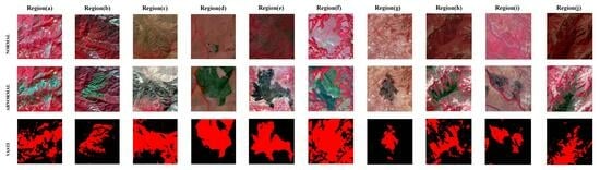
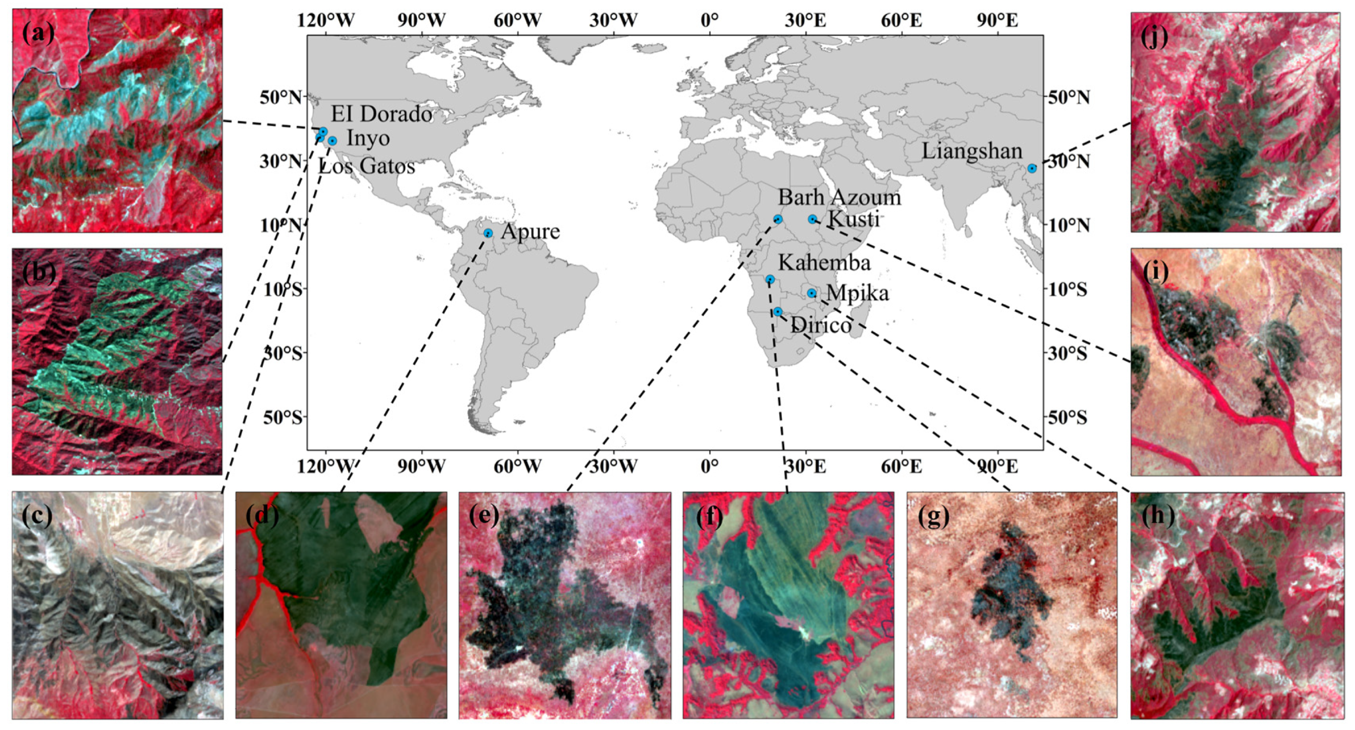
2.1. Abnormal Vegetation Satellite Dataset

The Landsat-8 satellite consists of two sensors, the Thermal Infrared Sensor (TIRS) and the Operational Land Imager (OLI). The OLI captures image data from nine spectral bands, while the TIRS collects image information from two thermal bands [37]. The Landsat-8 OLI images used in this study were downloaded from the U.S. Geological Survey (USGS) website (https://earthexplorer.usgs.gov/, accessed on 6 September 2022). Based on the 2016 fire point information from the Global Fire Atlas (GFA) [38], we chose ten research sites worldwide including six different land cover types to create a burned vegetation dataset. The distribution of these sites is illustrated in Figure 1. We systematically distinguished and identified burned areas at each of the ten sites to produce a comprehensive dataset of 1772 samples. The dataset has 3554 images in total, and each sample pair comprises two Landsat-8 optical images at a spatial resolution of 30 m. These images were captured before and after a fire incident in the same region.

Table 1. Dataset site details.

Site Name	Longitude	Latitude	Land Cover Type	Number of Samples	Sample Size
EI Dorado	120.8235°W	38.9682°N	Mixed forest	163	200 × 200
Los Gatos	121.8273°W	37.1111°N	Evergreen Needleleaf forest	52	200 × 200
Inyo	117.9242°W	36.0431°N	Evergreen Needleleaf forest	147	200 × 200
Apure	69.2507°W	7.2310°N	Grasslands	186	200 × 200
Barh Azoum	21.3424°E	11.5677°N	Savannas	223	200 × 200
Kahemba	18.8686°E	7.2313°S	Woody savannas	217	200 × 200
Dirico	21.2766°E	17.3446°S	Savannas	267	200 × 200
Mpika	31.8310°E	11.5675°S	Woody savannas	236	200 × 200
Kusti	32.0963°E	11.5679°N	Croplands	252	200 × 200
Liangshan	100.7287°E	27.4312°N	Evergreen Needleleaf forest	29	200 × 200

provides detailed information on the ten research sites, including names, coordinates, land cover types, and sample sizes. To find appropriate spectral and textural features for constructing the novel index, this dataset was used to statistically examine the changes in spectral and textural features before and after fires. The accuracy verification and performance assessment of the novel index were conducted by using a representative subset selected from the samples of each site.

2.2. Data Processing

After choosing the study sites based on latitudinal and longitudinal coordinates and along with the start and end times of large-scale fires in the GFA, we visually interpreted the dual-temporal remote sensing images at each site and labeled the burned vegetation areas. Both the images and the labels were then segmented into fixed-size 200 × 200 pixels. These segments underwent an assessment procedure, where regions with more than 80% mask coverage were designated as abnormal vegetation samples, to construct an abnormal vegetation database. Using pre-fire photos, a matching database of normal vegetation samples was concurrently generated for every abnormal vegetation segment. Based on this supplemental dataset, we computed the alterations in texture features after a wildfire and identified those texture features that exhibited outstanding discriminatory capabilities.

The processes of selecting data, analyzing images, identifying anomalies, and creating databases for both normal and abnormal vegetation samples were included the initial phases of the integrated data processing workflow. The dataset was used in further studies, including calculating changes in textural and spectral features before and after fires and identifying highly separable features.

3. Methodology

3.1. Selection of Texture Features

3.1.1. GLCM and Parameter Settings

In this study, we used the GLCM to calculate the texture features of vegetation samples. The GLCM is a statistical tool for elucidating the relationship between pixel gray levels within digital images [39]. The GLCM effectively captures the interplay among pixel pairs within an image, with a specific focus on quantifying the probabilities of gray-level co-occurrences among adjacent pixels along predefined directions. Principally, the GLCM counts the frequency with which certain pixel brightness value combinations appear in an image, serving as a fundamental method for extracting texture features, and has widespread classification applications in satellite images [40,41], computer vision [42,43], and other fields.

The computation of the GLCM involves four critical parameters: the orientation value, the displacement value d, the sliding window size, and the gray level. In practical situations, computational instability occurs from the significant manipulation of these four parameters in the GLCM. To illustrate the principles underlying GLCM computation, we employed a 6 × 6 image with eight gray levels as a demonstrative example. In this study, we outlined the methodology for calculating the GLCM, stipulating parameters such as distance (d = 1) and direction (θ = 0°). As shown in the sample image in Figure 2, pair (2,5), which is highlighted in red, occurred twice within a distance of 1 in the 0° direction. Consequently, the corresponding GLCM results are computed and depicted in Figure 3.

Due to the irregular spatial distribution and unfixed growth orientation of anomalous vegetation, we computed the average GLCM in four directions, 0°, 45°, 90°, and 135°, to mitigate the impact of potential errors stemming from calculating texture features in a single direction. Moreover, we set the window displacement step size of the GLCM to 1 to enable pixel-wise analysis of the relationships between each pixel and its surrounding pixels. This approach facilitates a more precise exploration of texture distinctions between normal and anomalous vegetation. The window size and gray levels for texture features depend on the properties of the terrestrial object and the spatial resolution of the remote sensing images. Hence, we conducted comparative experiments to identify the optimal parameter combinations. Under fixed conditions (average of the GLCM in four directions and step size of 1), we tested the performance of different sliding window sizes (3, 5, 7, 9, 11, 13, and 15) and different gray levels (16, 32, 64, 128, and 256).

Figure 4i presents the classification accuracies and kappa coefficients for normal and abnormal samples under various sliding window sizes. It is evident that the classification accuracy gradually improved as the sliding window size increased from 3 to 7. The classification accuracy decreased as the window size increased from 7 to 15. Similarly, in Figure 4ii, the gray-level setting of 64 yielded the highest classification accuracy and kappa coefficient, with lower values observed for the other four gray-level settings. According to these experimental results, we established the following four parameter settings for GLCM computation: a gray level of 64, a window displacement size of 7, a step size of 1, and the average of the GLCM in four directions.

3.1.2. Separability Analysis of Texture Features

Different texture features reflect different information in the image. Therefore, selecting appropriate texture features in accordance with particular classification requirements is essential. This selection guarantees that during the classification process, the texture features effectively improve the separability between burned and normal vegetation.

Based on the GLCM, it is possible to calculate several attributes. Various GLCM attributes have been developed for detecting certain similarities and differences [39,44]. Those texture features, which are based on the GLCM, can be categorized into three general groups: contrast group, order group, and statistics group. In this study, we ultimately computed 9 common textural features for the normal and abnormal vegetation samples, including the mean, standard deviation, contrast, dissimilarity, homogeneity, energy, correlation, autocorrelation (AC), and entropy.

Table 2. The formulas for the nine textures and their representative meanings.

Texture	Formula	Meaning
Mean	${\displaystyle \sum _{i=0}^{N_{\mathrm{G}}-1}{\displaystyle \sum _{j=0}^{N_G-1}i\cdot f(i,j)}}$	Reflects the degree of texture rules. The more regular the texture is, the larger the mean, and the less clutter there is, the smaller the mean.
Standard Deviation	${\displaystyle \sum _{i=0}^{N_G-1}{\displaystyle \sum _{j=0}^{N_G-1}{(i-\mu )}^{2}f(i,j}})$	Reflects the mean deviation and the value of each pixel in the image.
Contrast	${\displaystyle \sum _{i=0}^{N_G-1}{\displaystyle \sum _{j=0}^{N_G-1}{(i-j)}^{2}f(i,j}})$	Reflects the depth of the textural groove and the image sharpness. The visual impact is more distinct when the texture groove is deeper.
Dissimilarity	${\displaystyle \sum _{i=0}^{N_G-1}{\displaystyle \sum _{j=0}^{N_G-1}\left|i-j\right|f(i,j}})$	Similar to the contrast, a higher local contrast indicates a higher dissimilarity.
Homogeneity	${\displaystyle \sum _{i=0}^{N_G-1}{\displaystyle \sum _{j=0}^{N_G-1}\frac{f(i,j)}{1+{(i-j)}^2}}}$	Reflects the uniformity of the local grayscale of the image. The more uniform the grayscale is, the larger the cooperativity value.
Energy	${\displaystyle \sum _{i=0}^{N_G-1}{\displaystyle \sum _{j=0}^{N_G-1}f(i,j}}{)}^2$	Reflects the uniformity of the image gray distribution. The more uniform the gray distribution of the image is, the larger the energy value.
Correlation	${\displaystyle \sum _{i=0}^{N_G-1}{\displaystyle \sum _{j=0}^{N_G-1}\frac{(i-\mu )(j-\mu )f(i,j{)}^2}{{\delta }^2}}}$	Reflects the local gray image correlation.
Autocorrelation	${\displaystyle \sum _{i=0}^{N_G-1}{\displaystyle \sum _{j=0}^{N_G-1}(ij)f(i,j}})$	Reflects the consistency of the image texture.
Entropy	${\displaystyle \sum _{i=0}^{N_G-1}{\displaystyle \sum _{j=0}^{N_G-1}f(i,j)\lg f(i,j}})$	Reflects the randomness of the image texture. The information entropy is at its maximum if all the values in the symbiosis matrix are equal; if the values are unequal, the information entropy is small.

Note:$N_G$ is the number of gray levels, $f(i,j)$ is the entry (i, j) in the GLCM, $\mu$ is the GLCM mean, and ${\delta }^2$ is the GLCM variance.

displays the precise computation formulas and detailed information.

We mapped the statistical distributions of the different texture features and calculated the Bhattacharyya distance (B-distance) [45] to assess the separability of normal and abnormal vegetation. The B-distance is a metric for measuring the similarity between two probability distributions. Specifically, a larger B-distance indicates greater dissimilarity between two distributions. Figure 5 shows the kernel density of the nine texture features for the normal and anomalous vegetation samples. A higher B-distance indicates a stronger separable capacity for that particular texture feature. It is evident that the results for six texture features—contrast, dissimilarity, homogeneity, energy, correlation, and entropy—exhibit significant overlap between the normal and anomalous vegetation samples. Conversely, the B-distances for the mean, standard deviation, and AC are comparatively larger. Overall, as shown in Figure 5, AC emerges as the strongest discriminative texture feature that can separate abnormal areas from normal vegetation well. The selected AC texture feature is calculated to mitigate the instability arising from individual textures in anomaly detection.

3.2. Vegetation Indices Selection

3.2.1. Vegetation Indices Analysis

VIs are a crucial class of indicators that extract features from spectral reflectance data by combining two or more wavelengths associated with the biophysical characteristics of vegetation. These indices are widely applied in the field of vegetation to assess various aspects of vegetation, including health status, growth patterns, and coverage [46]. Currently, diverse kinds of VIs exist to accommodate distinct research requirements. In the domain of anomaly vegetation detection, hyperspectral imaging techniques, spectral attributes, various vegetation indices, and texture features have been comprehensively applied to enable the early identification of strawberry leaf diseases [47]. Furthermore, Buras et al. [48] quantified drought conditions across Europe in 2018 by specifically employing VIs such as the NDVI and EVI derived from MODIS. Additionally, Tavush et al. [49] used VIs such as the NDVI and MNDVI in conjunction with texture features from the GLCM for flood damage assessment during the Sardoba Dam breach incident.

In this study, we meticulously selected twelve widely employed VIs and computed them for individual research areas within twelve sample points from the dataset. Subsequently, we analyzed the separability of these computed results to identify the VIs that exhibit superior performance in recognizing vegetation anomaly areas. This step serves as a foundation for the subsequent development of a comprehensive spectral and textural vegetation anomaly index. The twelve VIs are calculated in

Table 3. Formulas for the twelve VIs.

VIs	Formula	References
NDVI	$({\rho }_{NIR}-{\rho }_{\mathrm{Re}d})/({\rho }_{NIR}+{\rho }_{\mathrm{Re}d})$	[50]
EVI	$2.5\times ({\rho }_{NIR}-{\rho }_{\mathrm{Re}d})/({\rho }_{NIR}+6\times {\rho }_{\mathrm{Re}d}-7.5\times {\rho }_{Blue}+1)$	[51]
RVI	${\rho }_{NIR}/{\rho }_{\mathrm{Re}d}$	[52]
GNDVI	$({\rho }_{NIR}-{\rho }_{Green})/({\rho }_{NIR}+{\rho }_{Green})$	[53]
TVI	$60\times ({\rho }_{NIR}-{\rho }_{Green})-100\times ({\rho }_{\mathrm{Re}d}-{\rho }_{Green})$	[54]
DVI	${\rho }_{NIR}-{\rho }_{\mathrm{Re}d}$	[55]
DSWI	$({\rho }_{NIR}+{\rho }_{Green})/({\rho }_{\mathrm{Re}d}+{\rho }_{SWIR1})$	[56]
MSAVI	$0.5\times (2\times {\rho }_{NIR}+1-\sqrt{{(2\times {\rho }_{NIR}+1)}^2-8\times ({\rho }_{NIR}-{\rho }_{\mathrm{Re}d})})$	[57]
GCVI	${\rho }_{NIR}/{\rho }_{Green}-1$	[58]
MSR	$({\rho }_{NIR}/{\rho }_{\mathrm{Re}d}-1)/\sqrt{{\rho }_{NIR}/{\rho }_{\mathrm{Re}d}+1}$	[59]
PBI	${\rho }_{NIR}/{\rho }_{Green}$	[60]
GEMI	$\eta \times (1-0.25\times \eta )-({\rho }_{\mathrm{Re}d}-0.125)/(1-{\rho }_{\mathrm{Re}d})$ $\eta =(2\times {\rho }_{NIR}^2-{\rho }_{\mathrm{Re}d}^2+1.5\times {\rho }_{NIR}+0.5\times {\rho }_{\mathrm{Re}d})/({\rho }_{NIR}+{\rho }_{\mathrm{Re}d}+0.5)$	[61]

Note: In these formulas, ${\rho }_{Blue}$, ${\rho }_{Green}$, ${\rho }_{\mathrm{Re}d}$, and ${\rho }_{NIR}$ represent the reflectance of the corresponding bands.

.

The M-index [62] was used to analyze the separability of the 12 VIs. The separability of the VIs depends on the variances of normal and abnormal vegetation areas. When the calculated M value of a vegetation index is greater than 1, the vegetation index is considered to have good separability. Conversely, a computed M-index of less than 1 indicates poor separability. Additionally, a higher M-index indicates better separability of the corresponding vegetation index for burned vegetation. The formula for the M-index is as follows:

$$M=\frac{\left|{\mu }_1-{\mu }_2\right|}{{\sigma }_1+{\sigma }_2}$$

(1)

where ${\mu }_1$ and ${\mu }_2$ represent the mean index values for abnormal vegetation areas and normal vegetation areas, respectively, and ${\sigma }_1$ and ${\sigma }_2$ represent the standard deviations for the two categories in an image.

3.2.2. Separability Analysis of VIs

The exceptional Vegetation Anomaly Spectral Texture Index (VASTI) is anticipated to effectively reduce intraclass variations while maximizing interclass differences. In other words, VASTI aims not only to highlight abnormal vegetation areas but also to significantly enhance the contrast between abnormal vegetation areas and normal vegetation areas. To achieve this objective, we analyzed the results from 12 different VIs calculated for 10 study regions. These ten study regions encompass a diverse range of vegetation cover types, including mixed forest, evergreen needle leaf forest, grasslands, savannas, woody savannas, and croplands. The study regions, which have diverse vegetation cover types, were intentionally chosen to reduce the influence of vegetation types on the extraction results of the VIs. To evaluate the quantitative separability between different VIs for burned vegetation, we employed the M-index to measure the separability between the histograms of two distinct vegetation states for the 10 selected study regions. The outcomes are displayed in Figure 6.

As shown in Figure 6, except for regions (e) and (f), the EVI exhibited the highest M-index values, which were ranked first among the 12 VIs. On the other hand, the M-index values of the GEMI ranked second in regions (a–d), and (j) while surpassing the EVI and ranked first in regions (e) and (f). Although the GEMI ranked third in terms of separability in study area (g) and fourth in areas (h) and (i), the separability of the other VIs relative to that of the GEMI in these regions was not stable and was even worse in some cases. Consequently, considering the comprehensive analysis of the separability results for the 12 VIs, both the EVI and GEMI demonstrated the highest and most stable separability in the 10 study regions. Additionally, the EVI highlighted the abnormal vegetation areas with minimum values, while the GEMI accentuated them with maximum values. Hence, these two VIs, which were selected by utilizing the concept of amplifying differences between normal and anomalous vegetation, were employed in a composite calculation to construct the Vegetation Amplitude Spectral Index (VASI). This index was subsequently incorporated into the construction of the VASTI, thereby amplifying the distinctions between two distinct states of vegetation and significantly enhancing the effectiveness of the VASTI in the identification of anomalous vegetation regions.

3.3. Vegetation Anomaly Spectral Texture Index

Principally, we aimed to develop a novel index for extracting abnormal vegetation areas. The principle behind developing this index is to amplify the differences between normal and anomalous vegetation, thereby highlighting anomalies. We performed a ratio operation between texture features and spectral features, explicitly integrating traditional vegetation indices with spatial texture information.

$$VASTI=\frac{VATI+1}{VASI+1}$$

(2)

The VATSI comprises the VASI and the Vegetation Anomaly Texture Index (VATI). Nine texture features were computed in this study based on the GLCM, and the key feature included in the composite index was determined to be AC. Utilizing AC texture features, the VATI is computed by the following formula:

$$VATI=\frac{A{C}_{NIR}-A{C}_{\mathrm{Re}d}}{A{C}_{NIR}+A{C}_{\mathrm{Re}d}}$$

(3)

where $A{C}_{NIR}$ represents the AC texture feature in the near-infrared band of the sample image and $A{C}_{\mathrm{Re}\mathrm{d}}$ represents the AC texture feature in the red band.

According to Figure 6, we eventually chose the GEMI and the EVI as the basis for constructing the VASI. The computation process involved amplifying the differences observed in the study area images. Notably, the abnormal regions exhibited distinctively high values of the GEMI and low values of the EVI. Thus, we performed computations on these two VIs to enhance the differentiation between normal and abnormal regions, as represented by the following formula:

$$VASI=\frac{GEMI+1}{EVI+1}$$

(4)

The computation revealed that the VASI results exhibited a pronounced maximum in the recognition of anomalous areas, meaning that the pixel values in regions of abnormal vegetation were greater than those in normal vegetation areas. In contrast, the VATI results exhibited a distinct minimum in the image, indicating that the pixel values in regions of abnormal vegetation were much lower than those in normal vegetation areas. Following these results, we employed the concept of accentuating differences and combined the VASI and VATI through comprehensive operations to obtain the VASTI scores.

3.4. Validation Methods

Confusion matrices were used to validate the detection accuracy of the various anomalous vegetation regions, and three metrics—user’s accuracy (UA), producer’s accuracy (PA), and the kappa coefficient—were ultimately selected to comprehensively evaluate the extraction accuracy of the different indices. These metrics are calculated as follows:

$$UA=\frac{TP}{TP+FP}$$

(5)

$$PA=\frac{TP}{TP+FN}$$

(6)

$$Kappa=\frac{p_o-p_e}{1-p_e}$$

(7)

$$p_o=\frac{TP+TN}{TP+TN+FP+FN}$$

(8)

$$p_e=\frac{(TP+FN)\times (TP+FP)+(FN+TN)\times (TN+FP)}{N^2}$$

(9)

In the equations, $TP$ represents the number of pixels where both the image truths (ITs) and predictions are positive. $TN$ refers to the number of pixels where both the ITs and predictions are negative. $FN$ represents the number of pixels where the ITs are positive but are predicted to be negative. $FP$ represents the number of pixels where the ITs are negative but are predicted to be positive.

4. Evaluation of the VASTI

4.1. Mapping of the VASTI and Other Indices

The VATSI model was proposed for abnormal vegetation cover for further validation. Unlike previous approaches that rely solely on spectral or textural information, the VASTI preserves the universality of spectral indices while mitigating their instability when integrated with textural features. To validate the superior performance of the composite index VASTI in detecting anomalous vegetation over individual VIs or texture features, we computed extraction results for ten study areas using the GEMI, EVI, AC, and VASTI, followed by visual evaluation and accuracy comparisons for anomalous vegetation recognition in each study area.

Figure 7i,ii, respectively, present false-color optical images of ten study regions under normal and abnormal conditions. Figure 7iii–vi shows the GEMI, EVI, AC, and VASTI results, with red regions indicating areas of anomalous vegetation. Figure 7ii–iv indicates that two VIs exhibit excessively fragmented detection of anomalous regions, occasionally misclassifying normal vegetation as anomalous vegetation. Moreover, variations or similarities in reflectance across different land cover types may cause VIs to inaccurately identify non-vegetated land surfaces as anomalous vegetation; this phenomenon is particularly noticeable in study areas (a), (b), and (h). In Figure 7v, some minor anomalous vegetation areas were overlooked, while the primary regions of anomaly occurrence were highlighted because we employed a 7 × 7 sliding window instead of a pixelwise window for computation. Using texture features to detect abnormal vegetation may reduce false-positives to some extent but may also result in missed anomalous regions. On the other hand, the VASTI combines both spectral indices and textural features, effectively highlighting the primary anomalous regions while retaining fine-scale details to mitigate the occurrence of misclassification and omission.

4.2. Validation of the VASTI

4.2.1. Comparison with the Components of VASTI

Figure 8 shows the recognition accuracy statistics for study regions (a)–(j) under the four indices. Figure 6 and Figure 8 indicate a notable increase in the recognition accuracy of the VASTI for anomalous regions compared to that of the GEMI, EVI, and AC. The VASTI exhibited a 1.7% to 4.4% increase in UA compared to that of the two spectral indices, with a particularly notable improvement of 22% in the study area (b). Compared to that of the AC, the VASTI demonstrated even more substantial UA improvement. Except for regions (a), (b), (d), and (f), where the improvement was less than 10%, improvements ranging from 13.4% to 27.4% were noted in the remaining six study areas. The VASTI also outperformed the three individual indices in terms of the PA, with most extraction results showing an improvement of 5% to 8%. In study areas (b), (c), and (e), the VASTI achieved improvements of 8% to 11%. Similarly, for most of the VASTI extraction results, the kappa coefficient was 5% to 10% greater than that of individual VIs and up to 13% to 22% greater than that of individual texture feature extraction results.

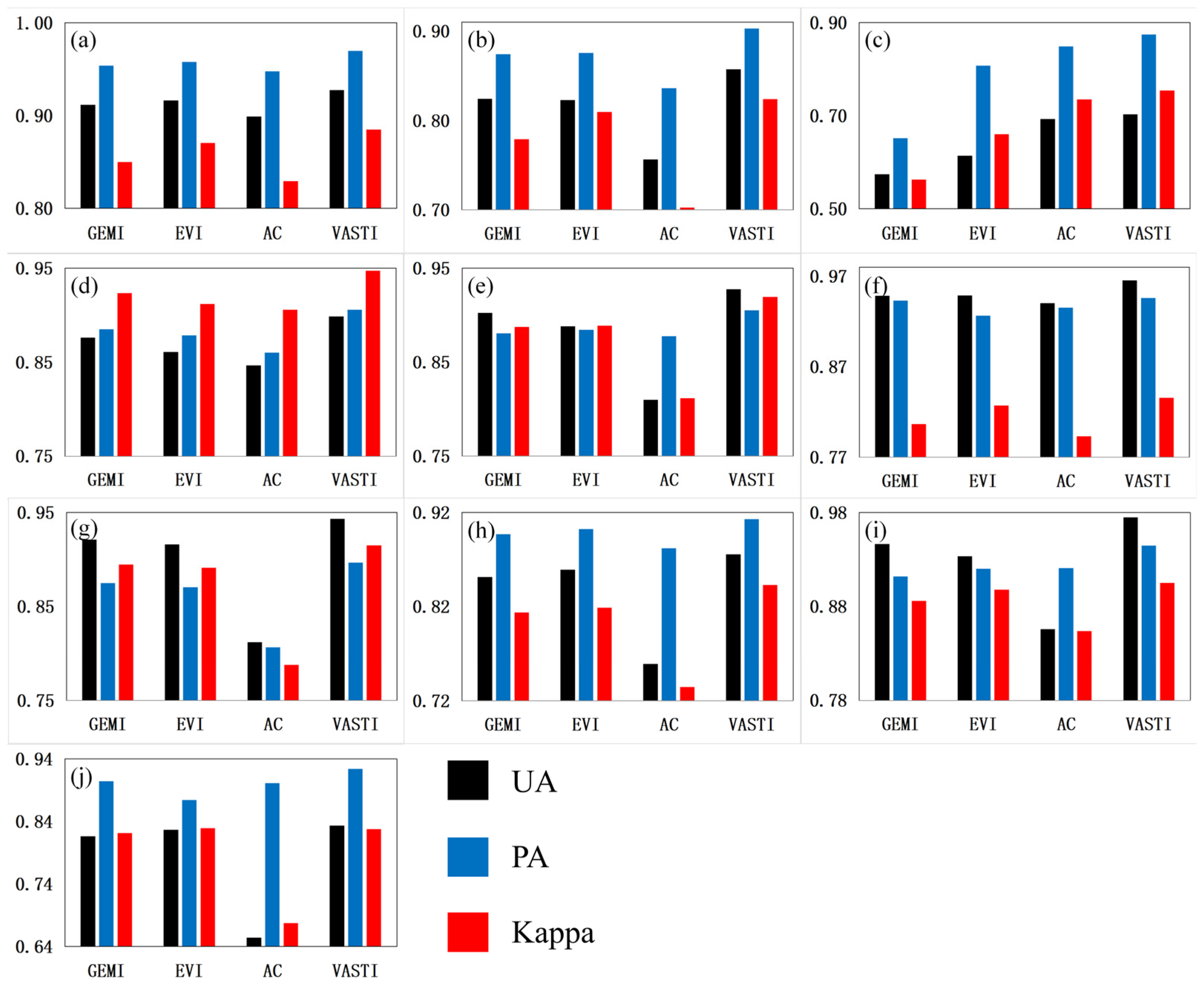
4.2.2. Comparison with Other Spectral and Textural Features

To validate the superior performance of VASTI in identifying fire-affected areas, this study not only contrasted it with three constituent indices but also conducted accuracy comparisons of VASTI with all VIs and texture features mentioned in Table 2 and Table 3. In addition, we considered another spectral index, Normalized Burn Ratio (NBR, (${\rho }_{NIR}$ − ${\rho }_{SWIR}$)/(${\rho }_{NIR}$ + ${\rho }_{SWIR}$)), which is commonly used to extract the burned region. Fornacca [63] has demonstrated that NBR is one of the three best indicators for burn scar detection starting one year after the fire. Therefore, to verify the accuracy and robustness of VASTI constructed in this study, NBR was added to the subsequent accuracy verification and evaluation for comparison.

Figure 9 presents a heatmap of the three accuracy indicators for VASTI and other spectral and textural indices. Accuracy, depicted on the graph from low to high, is reflected in a color bar ranging from red to blue, with deeper shades of blue indicating higher accuracy. The left side of Figure 9 shows the accuracy of VIs for identifying anomalous areas, while on the right side, the texture features are shown. Figure 9 illustrates that the detection capability of VIs for anomalous areas is significantly higher than that of texture features. It can be seen that NBR does show better performance in identifying burned areas than the rest of the other VIs. However, VASTI integrates both types of indices, and apart from a slightly lower PA and Kappa for the region (b) compared to GCVI, VASTI demonstrates superior performance in identifying burned areas compared to single spectral and texture features.

5. Discussion

5.1. Improvement of Combining VIs and Texture Features

The use of VIs for burned area detection and mapping has a long history [64,65,66]. Using spectral information at various wavelengths in images is necessary for the spectral analysis of vegetation [67,68,69]. To improve the accuracy and stability of the VASTI in detecting abnormal vegetation areas, we chose two of the twelve commonly used VIs for construction. Although VIs are still widely used for studying vegetation fires, a single spectral index has a lower accuracy in extracting abnormal areas than does the VASTI, which incorporates textural features in this study. There is a fundamental limitation to the spectral information obtained from remote sensing images [70]. First, VIs rely entirely on spectral information in images; therefore, they are easily affected by spectral confusion between unburned shadow pixels caused by geographical shadow effects and burned non-shadow pixels, particularly in areas with diverse terrains [71]. Second, spectral confusion may arise at the boundaries of abnormal areas when unburned forest canopy vegetation masks the burnt surface area. Texture information can help minimize errors caused by this factor [72].

The addition of texture information served as a complement to the spectral features [73,74,75]. Texture features reflect spatial correlations between a central pixel and other pixels within a defined window and describe the co-occurrence relationships between pixels [76]. As demonstrated in Figure 8, although texture features are primarily focused on spatial information, they are not particularly good at detecting abnormal vegetation areas that have been affected by fires. Compared to those of the single spectral indices and the composite VASTI indices, the AC texture features used in this study exhibited greatly decreased recognition accuracy for burned vegetation areas. Figure 5 shows that while the AC exhibited the best separability for anomalous vegetation among the nine texture features in this study, there was still some overlap in the AC value range between normal and anomalous vegetation. This overlap may be attributed to the similarity in grayscale co-occurrences among pixels. Furthermore, spatial information generally poses greater challenges in quantitatively expressing variability, patterns, shapes, and sizes than spectral information [77].

The purpose of creating the VASTI is to complement spectral features and texture features as explicit parameters in the index construction. The presence of two VIs somewhat lessened the instability of the texture features, and the VASTI guaranteed the accuracy of spectral features in detecting burned vegetation areas. The integration of spectral and textural features in plant species classification studies can increase the accuracy of vegetation species classification by as much as 10% to 15% [78,79]. Based on the accuracy statistics in Figure 8, it is evident that the three evaluation criteria for VASTI extraction results showed an improvement of approximately 5% when compared to single spectral or texture features in the majority of the study areas, with an improvement of up to 22% in a few particular study areas. The results of the quantitative analysis showed that the accuracy of detecting burnt vegetation was effectively increased by the VASTI.

5.2. Uncertainties of the VASTI

The VASTI has merits in terms of abnormal vegetation extraction, but it should be noted that it still has some uncertainties due to the parameter setting of the GLCM and the characteristics of the spectral indices. Different parameter settings of the GLCM can result in different outcomes [42]. For example, any possible permutation or combination of these four parameters could lead to thousands of different results, which then impacts the numerical values and variations in texture features [80]. For this reason, the parameter settings of the GLCM represent a major source of uncertainty in the VASTI. Therefore, we gradually determined specific values for the four parameters to decrease the negative effect. In addition, various land cover types react differently to varying textural features, which means that the textural feature we chose is simply a relative characteristic of abnormal vegetation with significant distinction rather than an absolute characteristic [81].

Spectral information also introduced uncertainties in the VASTI for the extraction of burned areas. Atmospheric interference affects the spectral information obtained from imagery, which can cause errors when spectral indices are subsequently computed from band data [82]. Due to the inherent characteristics of vegetation, spectral indices must consider seasonality and vegetation type, and these two aspects may result in different GEMI and EVI values [83]. Moreover, a change in the VIs does not eliminate background noise, snow cover, aging vegetation, or other factors, so the impact of non-fire factors on the VASTI is impossible to control [84]. Additionally, when a burned region is hidden by an unburned canopy of forest vegetation, spectral confusion may occur at the margins of aberrant areas [72].

5.3. Merits and Limitations of the VASTI

The experimental results indicated that the newly proposed VASTI performed better than did current approaches that use only spectral or textural features. The primary merits of the VASTI can be summarized as follows. First, the development of the VASTI included spectral features together with spatial texture information. This comprehensive approach enabled us to consider the impact of fires on vegetation from various perspectives while reducing errors caused by spectral heterogeneity [85]. Second, the distinctiveness of the VASTI lies in its utilization of both spectral and textural information, which not only enhances the accuracy of identifying anomalous vegetation regions but also makes it more adaptable to varying land covers and topographic conditions. In complex terrain environments, the VASTI has demonstrated increased robustness in reducing the occurrence of commission and omission errors when identifying anomalous features. This comprehensive index added flexibility and diversity to the remote sensing image analysis, providing robust support for the identification of anomalous vegetation in practical applications. Finally, the construction method of the VASTI is relatively intuitive and does not require extensive computations. Compared to that of traditional machine learning methods, VASTI has a lower computational load so that it can be efficient and scalable for anomaly detection [34,86].

Despite the significant merits of the VASTI in the identification of anomalous vegetation areas, several limitations need to be noted. First, it should be acknowledged that the value range of abnormal areas calculated by the VASTI is not fixed. This finding implies that the performance of the VASTI may vary in different geographical contexts, which poses a challenge that requires further research and resolution. Second, this study was subject to specific conditions and time constraints, so the universality of the VASTI has not been extensively validated. Therefore, future research will focus on conducting additional experiments to comprehensively assess and validate the applicability of the VASTI in different scenarios, aiming to improve its robustness and reliability.

6. Conclusions

Wildfire incidence rates have grown rapidly on a global scale. Despite vegetation possessing some degree of self-regenerative capacity, the detection of fire-affected areas and the implementation of appropriate human interventions for restoration are imperative. The main research and conclusions are summarized as follows:

(1)

We systematically investigated the response of different spatial texture features and spectral features to vegetation fires, tested the separability of texture features and spectral features for anomalous vegetation, and ultimately introduced a novel explicit index (VASTI) that incorporates both texture and spectral information. Unlike conventional spectral VIs, the VASTI considers the spatial connections between anomalous pixels and surrounding areas.

(2)

The UA, PA, and kappa coefficient of the VASTI improved by 5–10% compared to those of the GEMI and EVI in terms of the recognition results for the majority of the study areas. In some regions, the recognition accuracy of the VASTI was enhanced by 13–25% compared to that of a single texture feature.

Overall, the VASTI has demonstrated its capacity to detect the distribution of burned vegetation in a timely and reliable manner on an extensive scale, and it presents a wealth of opportunities for mapping and analyzing burned vegetation worldwide.

References

1. Flannigan, M.; Amiro, B.; Logan, K.; Stocks, B.; Wotton, B. Forest fires and climate change in the 21st century. Mitig. Adapt. Strat. Glob. Chang. 2006, 186, 64–87. [Google Scholar] [CrossRef]
2. Chu, T.; Guo, X. Remote Sensing Techniques in Monitoring Post-Fire Effects and Patterns of Forest Recovery in Boreal Forest Regions: A Review. Remote Sens. 2014, 6, 470–520. [Google Scholar] [CrossRef]
3. Liu, S.C.; Zheng, Y.Z.; Dalponte, M.; Tong, X.H. A novel fire index-based burned area change detection approach using Landsat-8 OLI data. Eur. J. Remote Sens. 2020, 53, 104–112. [Google Scholar] [CrossRef]
4. Bowman, D.M.J.S.; Balch, J.K.; Artaxo, P.; Bond, W.J.; Carlson, J.M.; Cochrane, M.A.; D’Antonio, C.M.; DeFries, R.S.; Doyle, J.C.; Harrison, S.P.; et al. Fire in the Earth system. Science 2009, 324, 481–484. [Google Scholar] [CrossRef] [PubMed]
5. Chuvieco, E.; Congalton, R.G. Mapping and inventory of forest fires from digital processing of tm data. Geocarto Int. 1988, 3, 41–53. [Google Scholar] [CrossRef]
6. Pereira, J.M.C.; Sousa, A.M.O.; Sá, A.C.L.; Martín, M.P.; Chuvieco, E. Regional-scale burnt area mapping in Southern Europe using NOAA-AVHRR 1 km data. In Remote Sensing of Large Wildfires; Springer: Berlin/Heidelberg, Germany, 1999; pp. 139–155. [Google Scholar]
7. Mitri, G.H.; Gitas, I.Z. Fire type mapping using object-based classification of Ikonos imagery. Int. J. Wildland Fire 2006, 15, 457–462. [Google Scholar] [CrossRef]
8. Rogan, J.; Franklin, J. Mapping burn severity in southern California using spectral mixture analysis. IEEE Int. Symp. Geosci. Remote Sens. 2001, 4, 1681–1683. [Google Scholar]
9. Hilker, T.; Wulder, M.A.; Coops, N.C.; Linke, J.; McDermid, G.; Masek, J.G.; Gao, F.; White, J.C. A new data fusion model for high spatial-and temporal-resolution mapping of forest disturbance based on Landsat and MODIS. Remote Sens. Environ. 2009, 113, 1613–1627. [Google Scholar] [CrossRef]
10. Mouillot, F.; Schultz, M.G.; Yue, C.; Cadule, P.; Tansey, K.; Ciais, P.; Chuvieco, E. Ten years of global burned area products from spaceborne remote sensing—A review: Analysis of user needs and recommendations for future developments. Int. J. Appl. Earth Obs. Geoinf. 2014, 26, 64–79. [Google Scholar] [CrossRef]
11. Martín, M.P.; Gómez, I.; Chuvieco, E. Burnt Area Index (BAIM) for burned area discrimination at regional scale using MODIS data. For. Ecol. Manag. 2006, 234, S221. [Google Scholar] [CrossRef]
12. Quintano, C.; Fernández-Manso, A.; Stein, A.; Bijker, W. Estimation of area burned by forest fires in Mediterranean countries: A remote sensing data mining perspective. For. Eco. Manag. 2011, 262, 1597–1607. [Google Scholar] [CrossRef]
13. Cahoon, D.R., Jr.; Stocks, B.J.; Levine, J.S.; Cofer, W.R., III; Pierson, J.M. Satellite analysis of the severe 1987 forest fires in northern China and southeastern Siberia. J. Geophys. Res. Atmos. 1994, 99, 18627–18638. [Google Scholar] [CrossRef]
14. Richards, J. Thematic mapping from multitemporal image data using the principal components transformation. Remote Sens. Environ. 1984, 16, 35–46. [Google Scholar] [CrossRef]
15. Smith, A.M.S.; Drake, N.A.; Wooster, M.J.; Hudak, A.T.; Holden, Z.A.; Gibbons, C.J. Production of Landsat ETM+ reference imagery of burned areas within Southern African savannahs: Comparison of methods and application to MODIS. Int. J. Remote Sens. 2007, 28, 2753–2775. [Google Scholar] [CrossRef]
16. Mukherjee, J.; Mukherjee, J.; Chakravarty, D. Detection of coal seam fires in summer seasons from Landsat 8 OLI/TIRS in Dhanbad. In Computer Vision, Pattern Recognition, Image Processing, and Graphics, Proceedings of the 6th National Conference, NCVPRIPG 2017, Mandi, India, 16–19 December 2017; Rameshan, R., Arora, C., Dutta Roy, S., Eds.; Communications in Computer and Information Science; Springer: Berlin/Heidelberg, Germany, 2018; Volume 841, pp. 529–539. [Google Scholar]
17. Quintano, C.; Fernández-Manso, A.; Fernández-Manso, O. Combination of Landsat and Sentinel-2 MSI Data for Initial Assessing of Burn Severity. Int. J. Appl. Earth Obs. Geoinf. 2018, 64, 221–225. [Google Scholar] [CrossRef]
18. Veraverbeke, S.; Verstraeten, W.; Lhermite, S.; Goossens, R. Evaluating Landsat thematic mapper spectral indices for estimating burn severity of the 2007 Peloponnese wildfires in Greece. Int. J. Wildland Fire 2010, 19, 558–569. [Google Scholar] [CrossRef]
19. Lhermitte, S.; Verbesselt, J.; Verstraeten, W.W.; Veraverbeke, S.; Coppin, P. Assessing intra-annual vegetation regrowth after fire using the pixel based regeneration index. J. Photogramm. Remote Sens. 2011, 66, 17–27. [Google Scholar] [CrossRef]
20. Fernández-García, V.; Kull, C.A. Refining historical burned area data from satellite observations. Int. J. Appl. Earth Obs. Geoinf. 2023, 120, 103350. [Google Scholar] [CrossRef]
21. Grigorov, B. GEMI—A Possible Tool for Identification of Disturbances in Confirerous Forests in Pernik Povince (Western Bulgaria). Civ. Environ. Eng. Rep. 2022, 32, 116–122. [Google Scholar] [CrossRef]
22. Veraverbeke, S.; Gitas, I.; Katagis, T.; Polychronaki, A.; Somers, B.; Goossens, R. Assessing post-fire vegetation recovery using red-near infrared vegetation indices: Accounting for background and vegetation variability. ISPRS J. Photogramm. Remote Sens. 2012, 68, 28–39. [Google Scholar] [CrossRef]
23. Laws, K.I. Textured Image Segmentation. Ph.D. Thesis, University of Southern California, Los Angeles, CA, USA, 1980. [Google Scholar]
24. Tuceryan, M.; Iain, A.K. Texture analysis. In Handbook of Pattern Recognition and Computer Vision; World Scientific Publishing: Singapore, 1993; pp. 235–276. [Google Scholar]
25. Hossain, K.; Parekh, R. Extending GLCM to include Color Information for Texture Recognition. AIP Conf. Proc. 2010, 1298, 583–588. [Google Scholar]
26. Tou, J.Y.; Tay, Y.H.; Lau, P.Y. One-dimensional Gray-level Co-occurrence Matrices for texture classification. In Proceedings of the 2008 International Symposium on Information Technology, Kuala Lumpur, Malaysia, 26–28 August 2008; pp. 1–6. [Google Scholar]
27. Smith, J.; Lin, T.; Ranson, K.J. The Lambertian Assumption and Landsat Data. Photogramm. Eng. Remote Sens. 1980, 46, 1183–1189. [Google Scholar]
28. Mitri, G.H.; Gitas, I.Z. A semi-automated object-oriented model for burned area mapping in the Mediterranean region using Landsat-TM imagery. Int. J. Wildland Fire 2004, 13, 367. [Google Scholar] [CrossRef]
29. Liu, L.; Chen, J.; Fieguth, P.; Zhao, G.; Chellappa, R.; Pietikäinen, M. From BoW to CNN: Two decades of texture representation for texture classification. Int. J. Comput. Vis. 2019, 127, 74–109. [Google Scholar] [CrossRef]
30. Seifi Majdar, R.; Ghassemian, H. A Probabilistic SVM Approach for Hyperspectral Image Classification Using Spectral and Texture Features. Int. J. Remote Sens. 2017, 38, 4265–4284. [Google Scholar] [CrossRef]
31. Li, C.; Liu, Q.; Li, B.; Liu, L. Investigation of Recognition and Classification of Forest Fires Based on Fusion Color and Textural Features of Images. Forests 2022, 13, 1719. [Google Scholar] [CrossRef]
32. Cao, X.; Chen, J.; Imura, H.; Higashi, O. An SVM-based method to extract urban areas from DMSP-OLS and SPOT VGT data. Remote Sens. Environ. 2009, 113, 2205–2209. [Google Scholar] [CrossRef]
33. Yankovich, E.P.; Yankovich, K.S.; Baranovskiy, N.V.; Bazarov, A.V.; Sychev, R.S.; Badmaev, N.B. Mapping of vegetation cover using Sentinel-2 to estimate forest fire danger. In Proceedings of the Remote Sensing of Clouds and the Atmosphere XXIV, Strasbourg, France, 9–12 September 2019; Volume 11152. [Google Scholar]
34. Mohammadpour, P.; Viegas, D.X.; Viegas, C. Vegetation mapping with random forest using sentinel 2 and GLCM texture feature—A case study for Lousã region, Portugal. Remote Sens. 2022, 14, 4585. [Google Scholar] [CrossRef]
35. Champion, I.; Dubois-Fernandez, P.; Guyon, D.; Cottrel, M. Radar image texture as a function of forest stand age. Int. J. Remote Sens. 2008, 29, 1795–1800. [Google Scholar] [CrossRef]
36. Niemi, M.T.; Vauhkonen, J. Extracting canopy surface texture from airborne laser scanning data for the supervised and unsupervised prediction of area-based forest characteristics. Remote Sens. 2016, 8, 582. [Google Scholar] [CrossRef]
37. Irons, J.R.; Dwyer, J.L.; Barsi, J.A. The next landsat satellite: The landsat data continuity mission. Remote Sens. Environ. 2012, 122, 11–21. [Google Scholar] [CrossRef]
38. Andela, N.; Morton, D.C.; Giglio, L.; Randerson, J.T. Global Fire Atlas with Characteristics of Individual Fires, 2003–2016; ORNL DAAC: Oak Ridge, TN, USA, 2019. [Google Scholar]
39. Haralick, R.M.; Shanmugam, K.; Dinstein, I. Textural Features for Image Classification. IEEE Trans. Syst. Man Cybern. 1973, 3, 610–621. [Google Scholar] [CrossRef]
40. Franklin, S.E.; Maudie, A.J.; Lavigne, M.B. Using spatial co-occurrence texture to increase forest structure and species composition classification accuracy. Photgrammetric Eng. Remote Sens. 2001, 67, 849–855. [Google Scholar]
41. Bai, Y.K.; Sun, G.M.; Li, Y.; Ma, P.F.; Li, G.; Zhang, Y.Z. Comprehensively analyzing optical and polarimetric SAR features for land-use/land-cover classification and urban vegetation extraction in highly-dense urban area. Int. J. Appl. Earth Obs. Geoinf. 2021, 103, 102496. [Google Scholar] [CrossRef]
42. Hall-Beyer, M. Practical guidelines for choosing GLCM textures to use in landscape classification tasks over a range of moderate spatial scales. Int. J. Remote Sens. 2017, 38, 1312–1338. [Google Scholar] [CrossRef]
43. Warner, T. Kernel-based texture in remote sensing image classification. Geogr. Compass. 2011, 5, 781–798. [Google Scholar] [CrossRef]
44. Conners, R.W.; Trivedi, M.M.; Harlow, C.A. Segmentation of a high-resolution urban scene using texture operators. Comput. Vis. Graph. Image Process. 1984, 25, 273–310. [Google Scholar] [CrossRef]
45. Bhattacharyya, A. On a measure of divergence between two multinomial populations. Indian. J. Stat. 1946, 7, 401–406. [Google Scholar]
46. Moghadam, P.; Ward, D.; Goan, E.; Jayawardena, S.; Sikka, P.; Hernandez, E. Plant Disease Detection Using Hyperspectral Imaging. In Proceedings of the International Conference on Digital Image Computing: Techniques and Applications (DICTA), Sydney, NSW, Australia, 29 November–1 December 2017. [Google Scholar]
47. Wu, G.S.; Fang, Y.L.; Jiang, Q.Y.; Cui, M.; Li, N.; Ou, Y.M.; Diao, Z.H.; Zhang, B.H. Early identification of strawberry leaves disease utilizing hyperspectral imaging combing with spectral features, multiple vegetation indices and textural features. Comput. Electron. Agric. 2023, 204, 107553. [Google Scholar] [CrossRef]
48. Buras, A.; Rammig, A.; Zang, C.S. Quantifying impacts of the 2018 drought on European ecosystems in comparison to 2003. Biogeosciences 2020, 17, 1655–1672. [Google Scholar] [CrossRef]
49. Tavus, B.; Kocaman, S.; Gokceoglu, C. Flood damage assessment with Sentinel-1 and Sentinel-2 data after Sardoba dam break with GLCM features and Random Forest method. Sci. Total Environ. 2022, 816, 151585. [Google Scholar] [CrossRef] [PubMed]
50. Carlson, T.N.; Ripley, D.A. On the Relation between NDVI, Fractional Vegetation Cover, and Leaf Area Index. Remote Sens. Environ. 1997, 62, 241–252. [Google Scholar] [CrossRef]
51. Liu, H.Q.; Huete, A. A feedback based modification of the NDVI to minimize canopy background and atmospheric noise. IEEE Trans. Geosci. Remote Sens. 1995, 33, 457–465. [Google Scholar] [CrossRef]
52. Pearson, R.L.; Miller, L.D. Remote Mapping of Standing Crop Biomass for Estimation of Productivity of the Shortgrass Prairie. In Proceedings of the Eighth International Symposium on Remote Sensing of Environment, Ann Arbor, MI, USA, 2–6 October 1972. [Google Scholar]
53. Gitelson, A.A.; Kaufman, Y.J.; Merzlyak, M.N. Use of a green channel in remote sensing of global vegetation from EOS-MODIS. Remote Sens. Environ. 1996, 58, 289–298. [Google Scholar] [CrossRef]
54. Broge, N.H.; Leblanc, E. Comparing Prediction Power and Stability of Broadband and Hyperspectral Vegetation Indices for Estimation of Green Leaf Area Index and Canopy Chlorophyll Density. Remote Sens. Environ. 2001, 76, 156–172. [Google Scholar] [CrossRef]
55. Jordan, C.F. Derivation of Leaf-Area Index from Quality of Light on the Forest Floor. Ecology 1969, 50, 663–666. [Google Scholar] [CrossRef]
56. Galvão, L.S.; Formaggio, A.R.; Tisot, D.A. Discrimination of sugarcane varieties in Southeastern Brazil with EO-1 Hyperion data. Remote Sens. Environ. 2005, 94, 523–534. [Google Scholar] [CrossRef]
57. Qi, J.; Chehbouni, A.; Huete, A.R.; Kerr, Y.H.; Sorooshian, S. A modified soil adjusted vegetation index. Remote Sens. Environ. 1994, 48, 119–126. [Google Scholar] [CrossRef]
58. Gitelson, A.A.; Viña, A.; Arkebauer, T.J.; Rundquist, D.C.; Keydan, G.; Leavitt, B. Remote estimation of leaf area index and green leaf biomass in maize canopies. Geophys. Res. Lett. 2003, 30, 1248. [Google Scholar] [CrossRef]
59. Pu, R.; Gong, P.; Yu, Q. Comparative Analysis of EO-1 ALI and Hyperion, and Landsat ETM+ Data for Mapping Forest Crown Closure and Leaf Area Index. Sensors 2008, 8, 3744–3766. [Google Scholar] [CrossRef]
60. Nidamanuri, R.; Garg, P.K.; Sanjay, G.; Vinay, D. Estimation of leaf total chlorophyll and nitrogen concentrations using hyperspectral satellite imagery. J. Agric. Sci. 2008, 146, 65–75. [Google Scholar]
61. Pinty, B.; Verstraete, M.M. GEMI: A Non-Linear Index to Monitor Global Vegetation from Satellites. Vegetatio 1992, 101, 15–20. [Google Scholar] [CrossRef]
62. Kaufman, Y.J.; Remer, L.A. Detection of forests using mid-IR reflectance: An application for aerosol studies. IEEE Trans. Geosci. Remote Sens. 1994, 32, 672–683. [Google Scholar] [CrossRef]
63. Fornacca, D.; Ren, G.; Xiao, W. Evaluating the Best Spectral Indices for the Detection of Burn Scars at Several Post-Fire Dates in a Mountainous Region of Northwest Yunnan, China. Remote Sens. 2018, 10, 1196. [Google Scholar] [CrossRef]
64. Barbosa, P.M.; Grégoire, J.-M.; Pereira, J.M.C. An algorithm for extracting burned areas from time series of AVHRR GAC data applied at a continental scale. Remote Sens. Environ. 1990, 69, 253–263. [Google Scholar] [CrossRef]
65. Chafer, C.J.; Noonan, M.; Macnaught, E. The post-fire measurement of fire severity and intensity in the Christmas 2001 Sydney wildfires. Int. J. Wildland Fire 2004, 13, 227–240. [Google Scholar] [CrossRef]
66. French, N.H.F.; Kasischke, E.S.; Hall, R.J.; Murphy, K.A.; Verbyla, D.L.; Hoy, E.E.; Allen, J.L. Using Landsat data to assess fire and burn severity in the North American boreal forest region: An overview and summary of results. Int. J. Wildland Fire 2008, 17, 443–462. [Google Scholar] [CrossRef]
67. Chuvieco, E.; Opazo, S.; Sione, W.; Valle, H.D.; Anaya, J.; Di Bella, C.; Cruz, I.; Manzo, L.; Lopez, G.; Mari, N.; et al. Global burned-land estimation in Latin America using MODIS composite data. Ecol. Appl. 2008, 18, 64–79. [Google Scholar] [CrossRef]
68. Hantson, S.; Padilla, M.; Corti, D.; Chuvieco, E. Strengths and weaknesses of MODIS hotspots to characterize global fire occurrence. Remote Sens. Environ. 2013, 131, 152–159. [Google Scholar] [CrossRef]
69. Chuvieco, E.; Mouillot, F.; van der Werf, G.R.; San Miguel, J.; Tanase, M.; Koutsias, N.; García, M.; Yebra, M.; Padilla, M.; Gitas, I.; et al. Historical background and current developments for mapping burned area from satellite Earth observation. Remote Sens. Environ. 2019, 225, 45–64. [Google Scholar] [CrossRef]
70. Ghasemi, N.; Sahebi, M.R.; Mohammadzadeh, A. Biomass Estimation of a Temperate Deciduous Forest Using Wavelet Analysis. IEEE Trans. Geosci. Remote Sens. 2013, 51, 765–776. [Google Scholar] [CrossRef]
71. Wu, Z.; He, H.; Liang, Y.; Cai, L.; Lewis, B. Determining relative contributions of vegetation and topography to burn severity from LANDSAT imagery. Environ. Manag. 2013, 52, 821–836. [Google Scholar] [CrossRef] [PubMed]
72. Yuan, J.; Wang, D.; Li, R. Remote sensing image segmentation by combining spectral and texture features. IEEE Trans. Geosci. Remote Sens. 2013, 52, 16–24. [Google Scholar] [CrossRef]
73. Soh, L.-K.T.C. Texture analysis of sar sea ice imagery using gray level co-occurrence matrices. IEEE Trans. Geosci. Remote Sens. 1999, 37, 780–795. [Google Scholar] [CrossRef]
74. Ozdemir, I.; Karnieli, A. Predicting Forest Structural Parameters Using the Image Texture Derived from WorldView-2 Multispectral Imagery in a Dryland Forest, Israel. Int. J. Appl. Earth Obs. Geoinf. 2011, 13, 701–710. [Google Scholar] [CrossRef]
75. Fang, G.; He, X.; Weng, Y.; Fang, L. Texture Features Derived from Sentinel-2 Vegetation Indices for Estimating and Mapping Forest Growing Stock Volume. Remote Sens. 2023, 15, 2821. [Google Scholar] [CrossRef]
76. Baraldi, A.; Parmiggiani, F. Investigation of the textural characteristics associated with gray level cooccurrence matrix statistical parameters. IEEE Trans. Geosci. Remote Sens. 1995, 33, 293–304. [Google Scholar] [CrossRef]
77. Duan, M.; Zhang, X. Using remote sensing to identify soil types based on multiscale image texture features. Comput. Electron. Agric. 2021, 187, 106272. [Google Scholar] [CrossRef]
78. Wessel, M.; Brandmeier, M.; Tiede, D. Evaluation of Different Machine Learning Algorithms for Scalable Classification of Tree Types and Tree Species Based on Sentinel-2 Data. Remote Sens. 2018, 10, 1419. [Google Scholar] [CrossRef]
79. Fassnacht, F.E.; Latifi, H.; Stereńczak, K.; Modzelewska, A.; Lefsky, M.; Waser, L.T.; Straub, C.; Ghosh, A. Review of studies on tree species classification from remotely sensed data. Remote Sens. Environ. 2016, 186, 64–87. [Google Scholar] [CrossRef]
80. Armi, L.; Fekri-Ershad, S. Texture image analysis and texture classification methods—A review. arXiv 2019, arXiv:1904.06554. [Google Scholar]
81. Guo, W.; Rees, W.G. Altitudinal forest-tundra ecotone categorisation using texture-based classification. Remote Sens. Environ. 2019, 232, 111312. [Google Scholar] [CrossRef]
82. Mangeon, S.; Field, R.; Fromm, M.; McHugh, C.; Voulgarakis, A. Satellite versus ground-based estimates of burned area: A comparison between MODIS based burned area and fire agency reports over North America in 2007. Anthr. Rev. 2015, 3, 76–92. [Google Scholar] [CrossRef]
83. Hansen, M.C.; Potapov, P.V.; Moore, R.; Hancher, M.; Turubanova, S.A.; Tyukavina, A.; Thau, D.; Stehman, S.V.; Goetz, S.J.; Loveland, T.E.; et al. High-Resolution Global Maps of 21st-Century Forest Cover Change. Science 2013, 342, 850–853. [Google Scholar] [CrossRef] [PubMed]
84. Fraser, R.H.; Li, Z.; Cihlar, J. Hotspot and NDVI Differencing Synergy (HANDS): A New Technique for Burned Area Mapping over Boreal Forest. Remote Sens. Environ. 2000, 74, 362–376. [Google Scholar] [CrossRef]
85. Mondini, C.A. Measures of Spatial Autocorrelation Changes in Multitemporal SAR Images for Event Landslides Detection. Remote Sens. 2017, 9, 554. [Google Scholar] [CrossRef]
86. Wu, D.R.; Linders, J. A new texture approach to discrimination of forest clearcut, canopy, and burned area using airborne C-band SAR. IEEE Trans. Geosci. Remote Sens. 1999, 37, 555–563. [Google Scholar]
Figure 1. Distribution map of the sample sites in the burned vegetation dataset. Region (aj) are the representative study areas, namely, EI Dorado, Los Gatos, Inyo, Apure, Barh Azoum, Kahemba, Dirico, Mpika, Kusti, and Liangshan, respectively, selected to validate the VASTI.
Remotesensing 16 01539 g001
Figure 2. Example image with 8 gray levels.
Remotesensing 16 01539 g002
Figure 3. The GLCM was constructed with an angle of 0° and a distance factor of 1.
Remotesensing 16 01539 g003
Figure 4. Comparison plot of different sliding window sizes and gray-level settings of the GLCM. The left axis of the graph represents the producer accuracy for different sizes of sliding windows or gray levels, while the right axis corresponds to the respective kappa coefficients; (i) shows the trends of the producer’s accuracy (PA) and kappa coefficient for the same texture feature in the same study area with the sliding window size of the GLCM; (ii) shows the trends of the PA and kappa coefficient for the same texture feature in the same study area with the gray level of the GLCM.
Remotesensing 16 01539 g004
Figure 5. Comparison map of nine texture features between normal vegetation and abnormal vegetation samples.
Remotesensing 16 01539 g005
Figure 6. Statistical map of the calculation results for the different VIs in each study area. (aj) is consistent with the study area codes in Figure 1.
Remotesensing 16 01539 g006
Figure 7. Mapping of the study areas in normal and abnormal situations visual results of the GEMI, EVI, AC, and VASTI. (aj) is consistent with the study area codes in Figure 1.
Remotesensing 16 01539 g007
Figure 8. Statistical maps of the UA, PA, and kappa coefficient of the four indices for extracting vegetation anomaly regions. (aj) is consistent with the study area codes in Figure 1.
Remotesensing 16 01539 g008
Figure 9. Heatmap visualization of VASTI compared to three different evaluation indicators of other spectral and textural features; (i) shows the comparison of UA; (ii) shows the comparison of PA; (iii) shows the comparison of the Kappa coefficient. (aj) is consistent with the study area codes in Figure 1.
Remotesensing 16 01539 g009