
Preflight Spectral Calibration of the Ozone Monitoring Suite-Nadir on FengYun 3F Satellite

 , , ,
, , ,  and
and 
Abstract
:1. Introduction
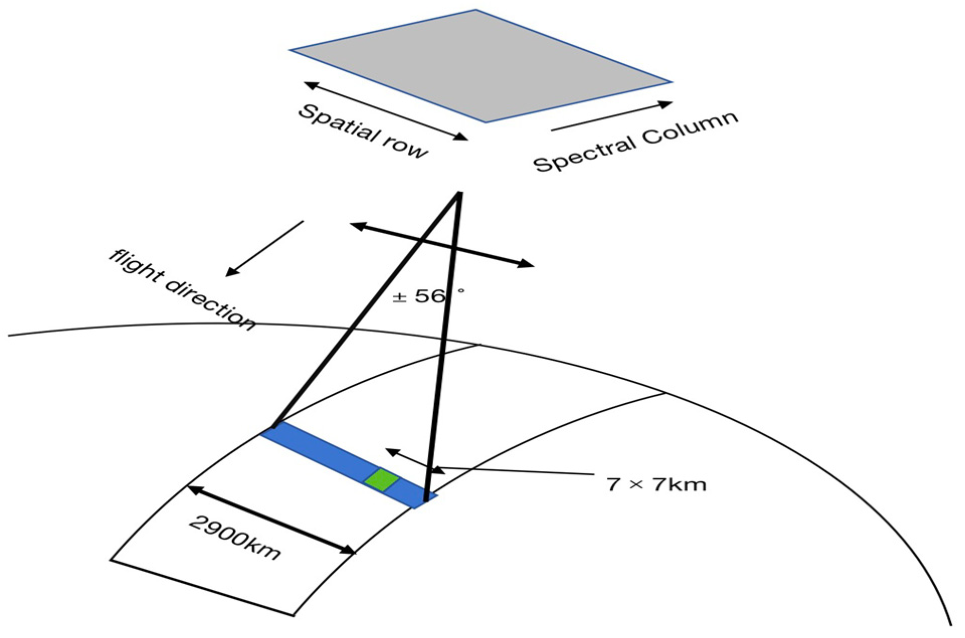
2. OMS-N Overview
3. Spectral Calibration Methodology
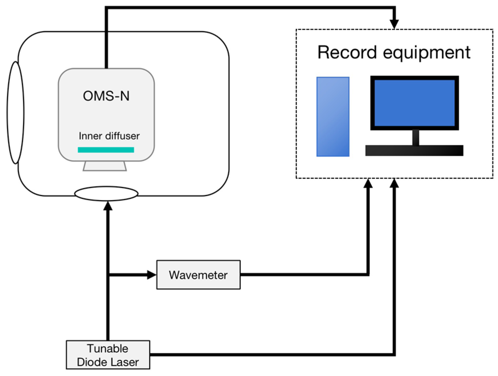
3.1. Method
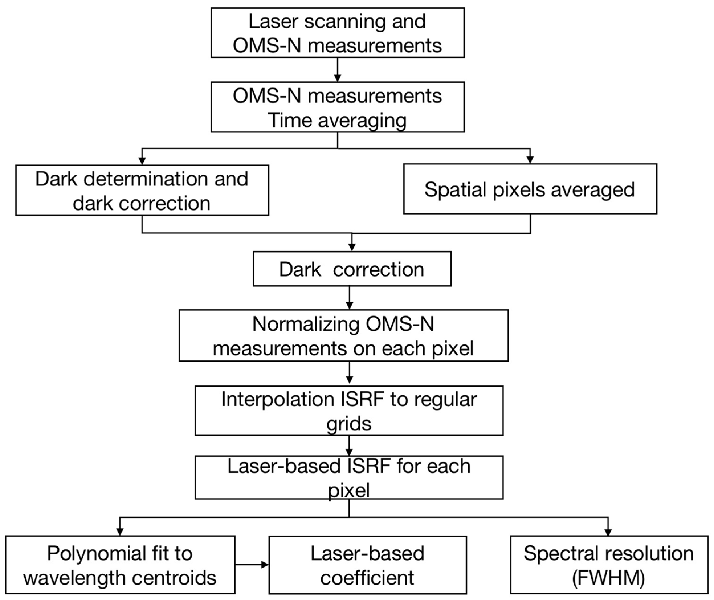
3.2. Data Processing
4. Results and Discussion
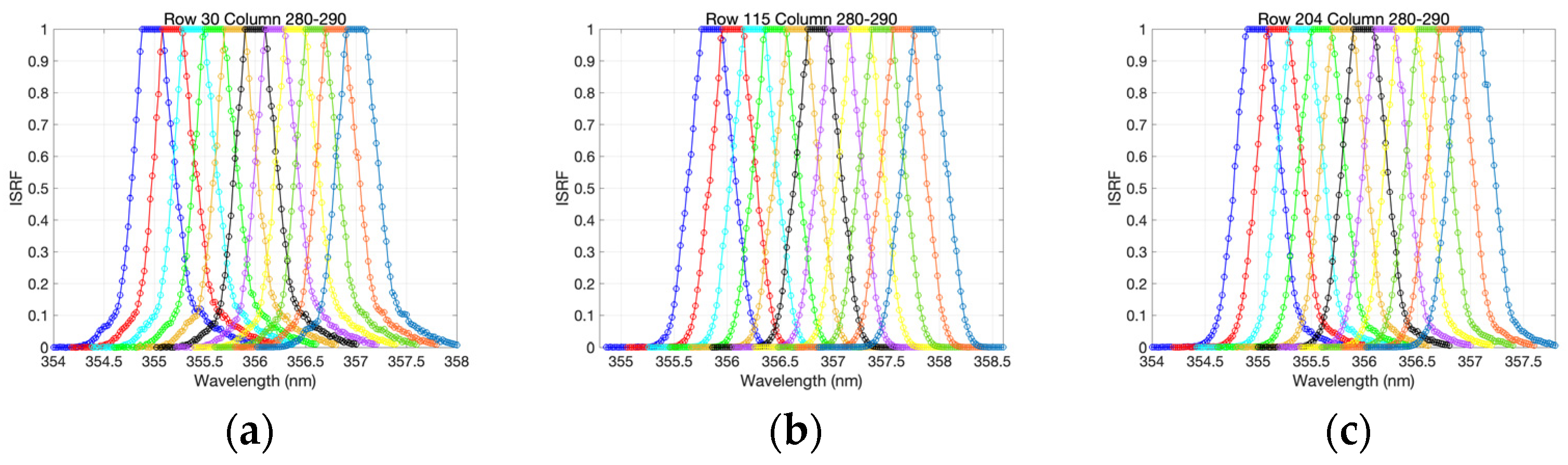
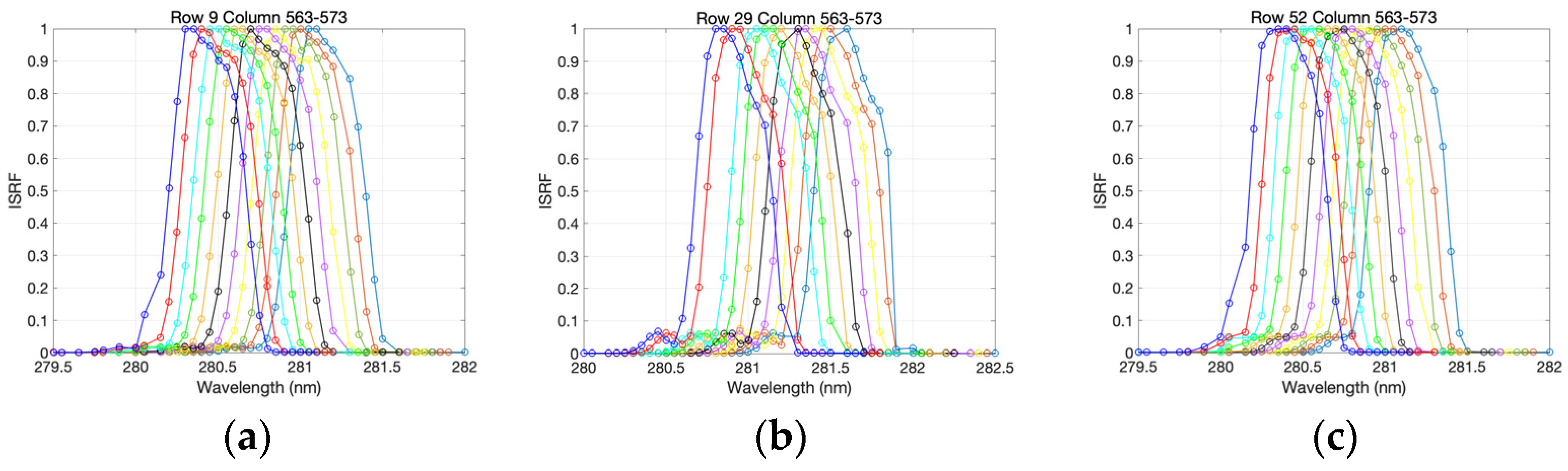
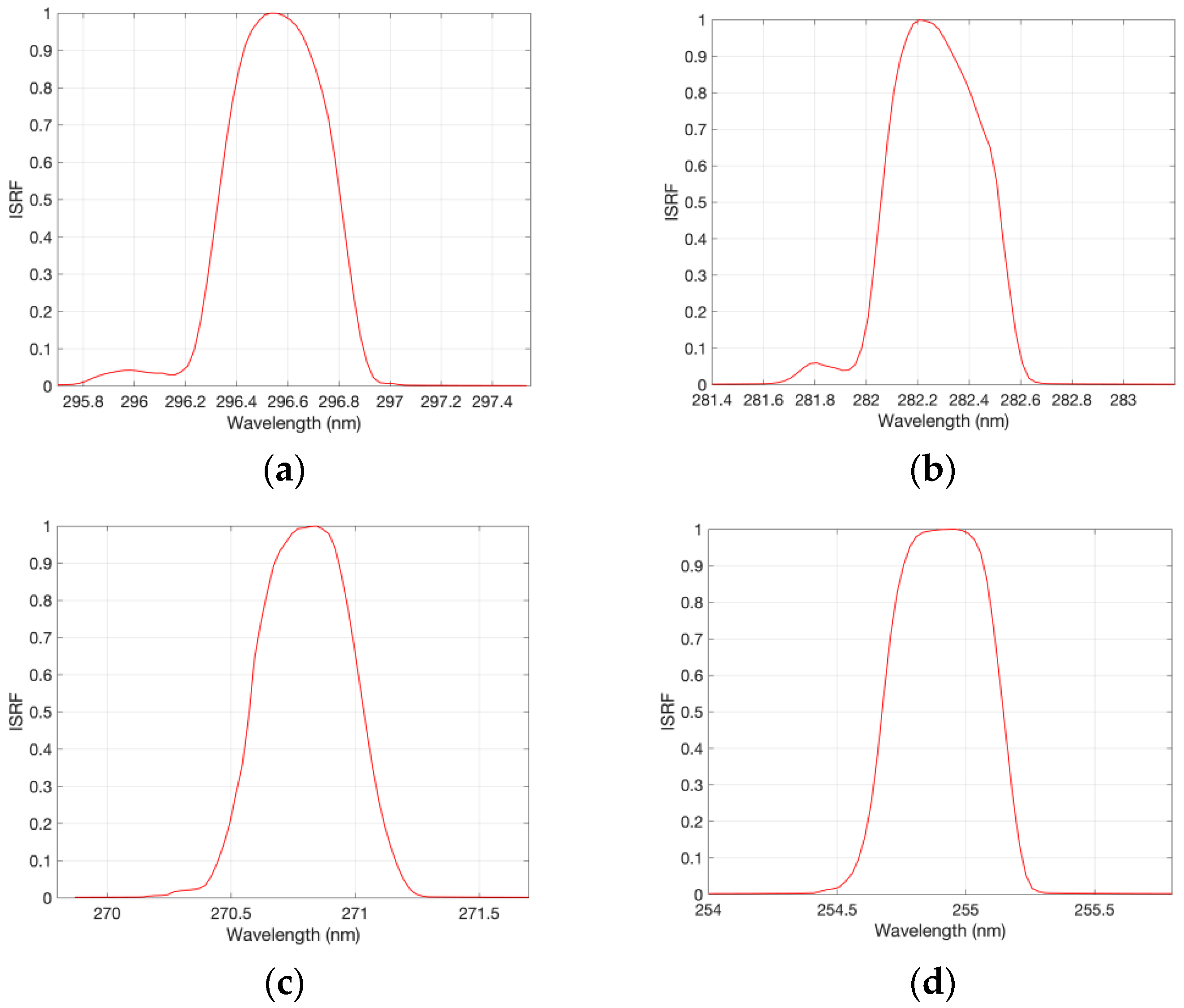
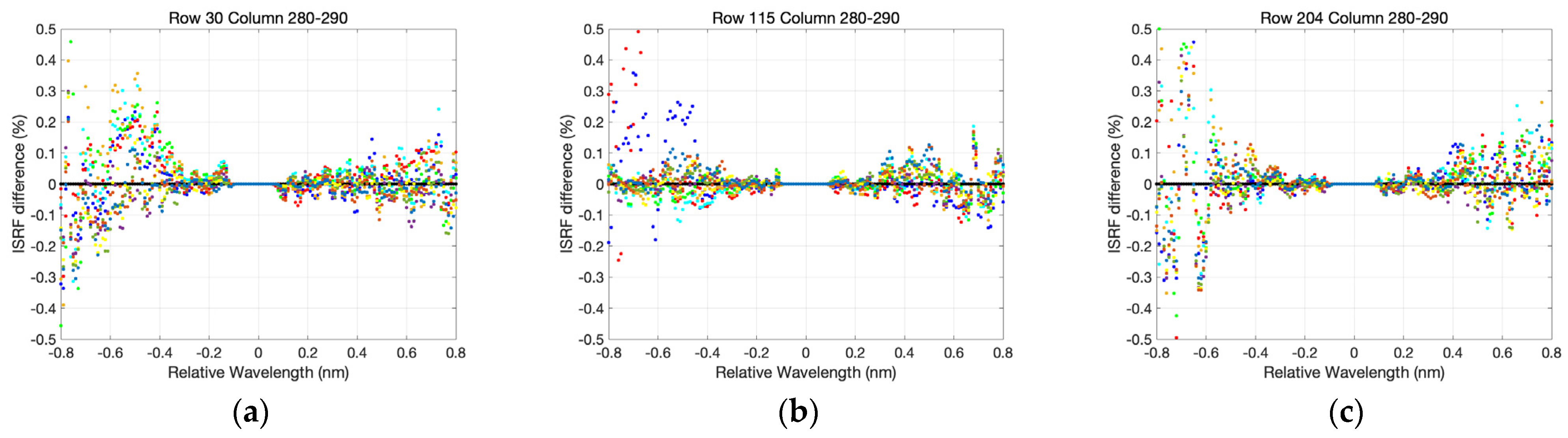
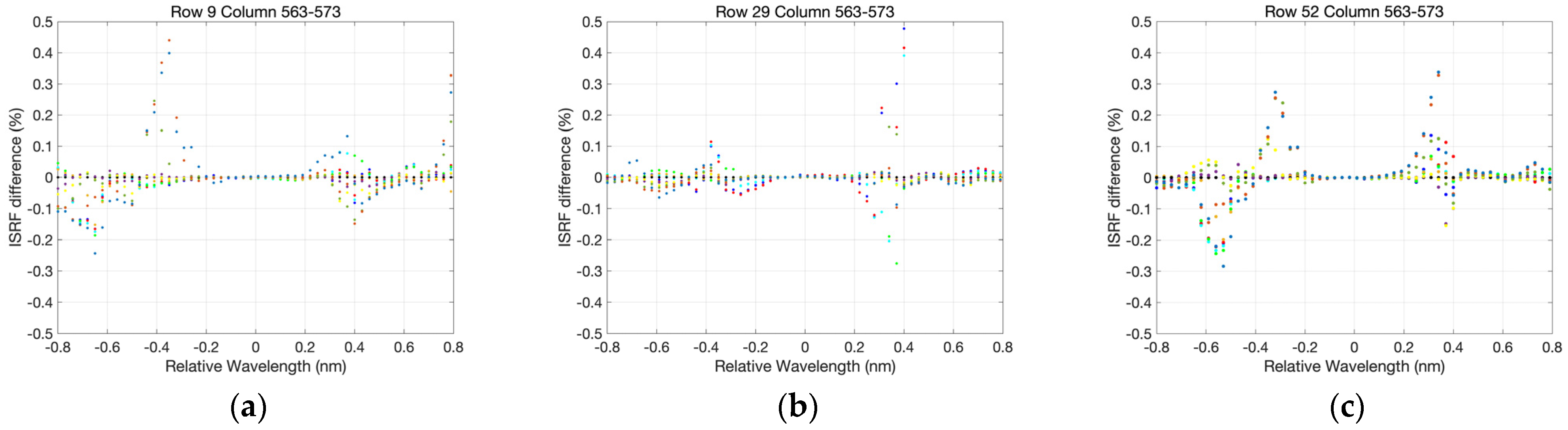
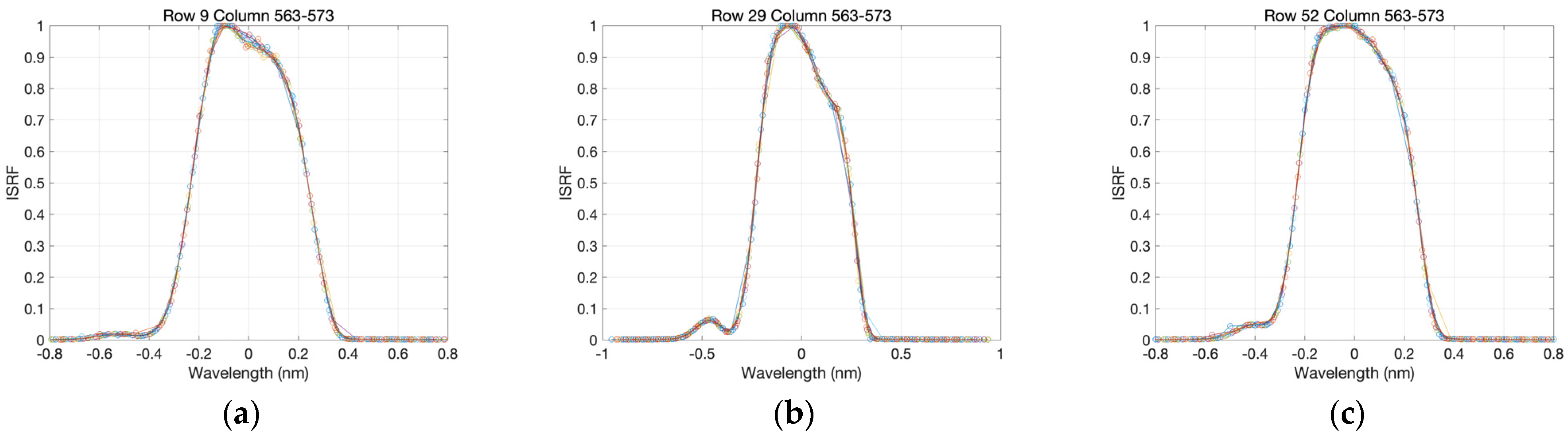
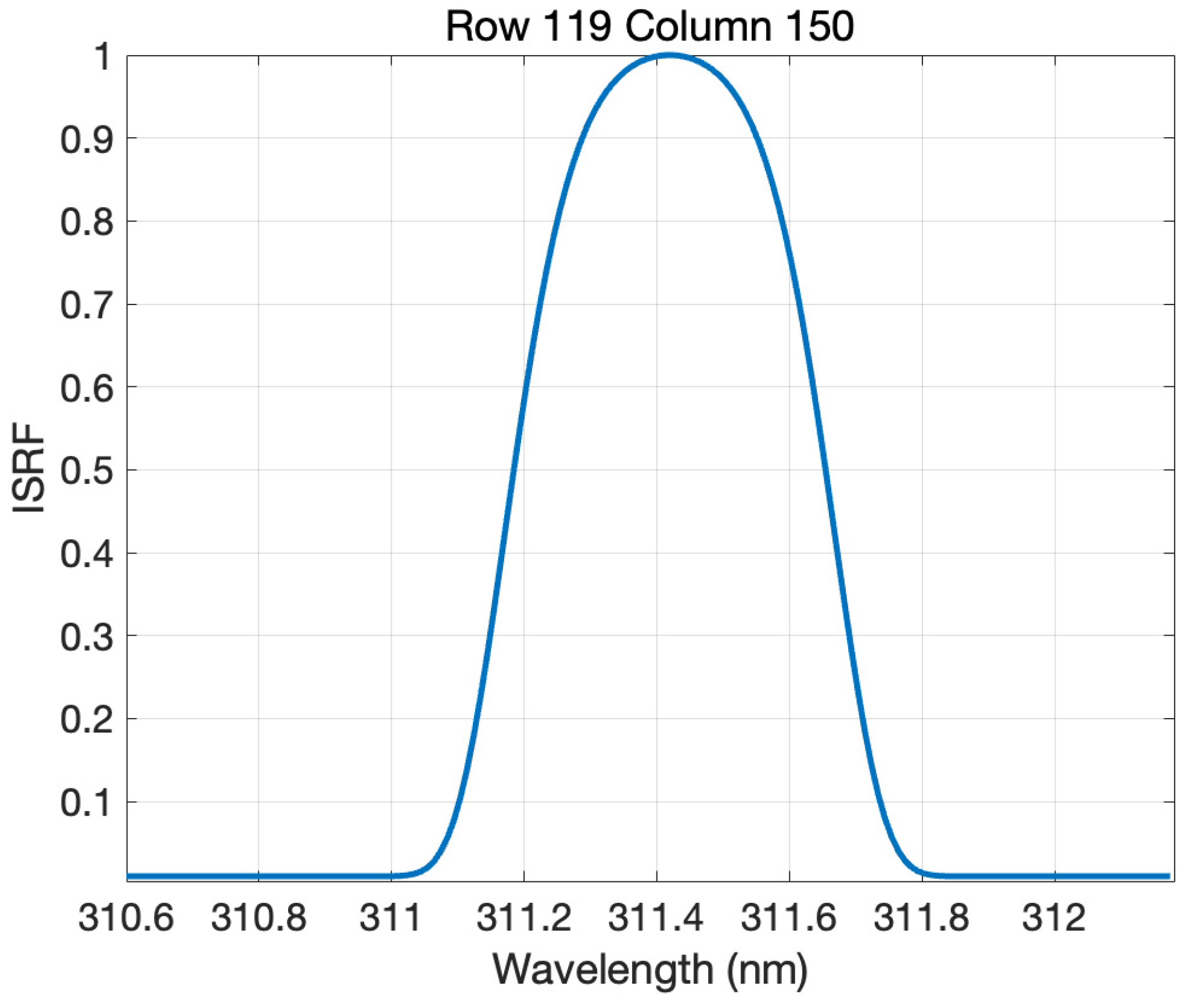
4.1. ISRF
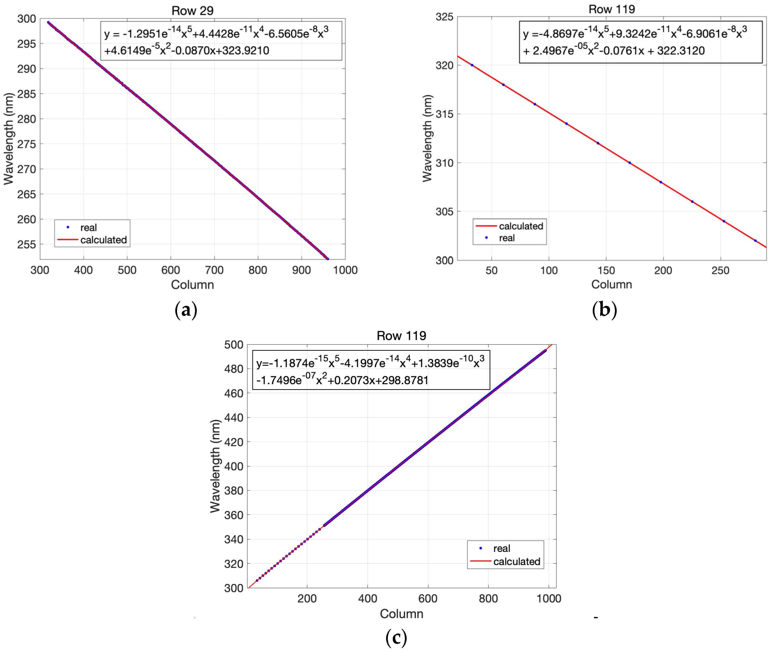
4.2. Spectral Dispersion
4.3. Spectral Resolution
4.4. Verification of Wavelength Accuracy
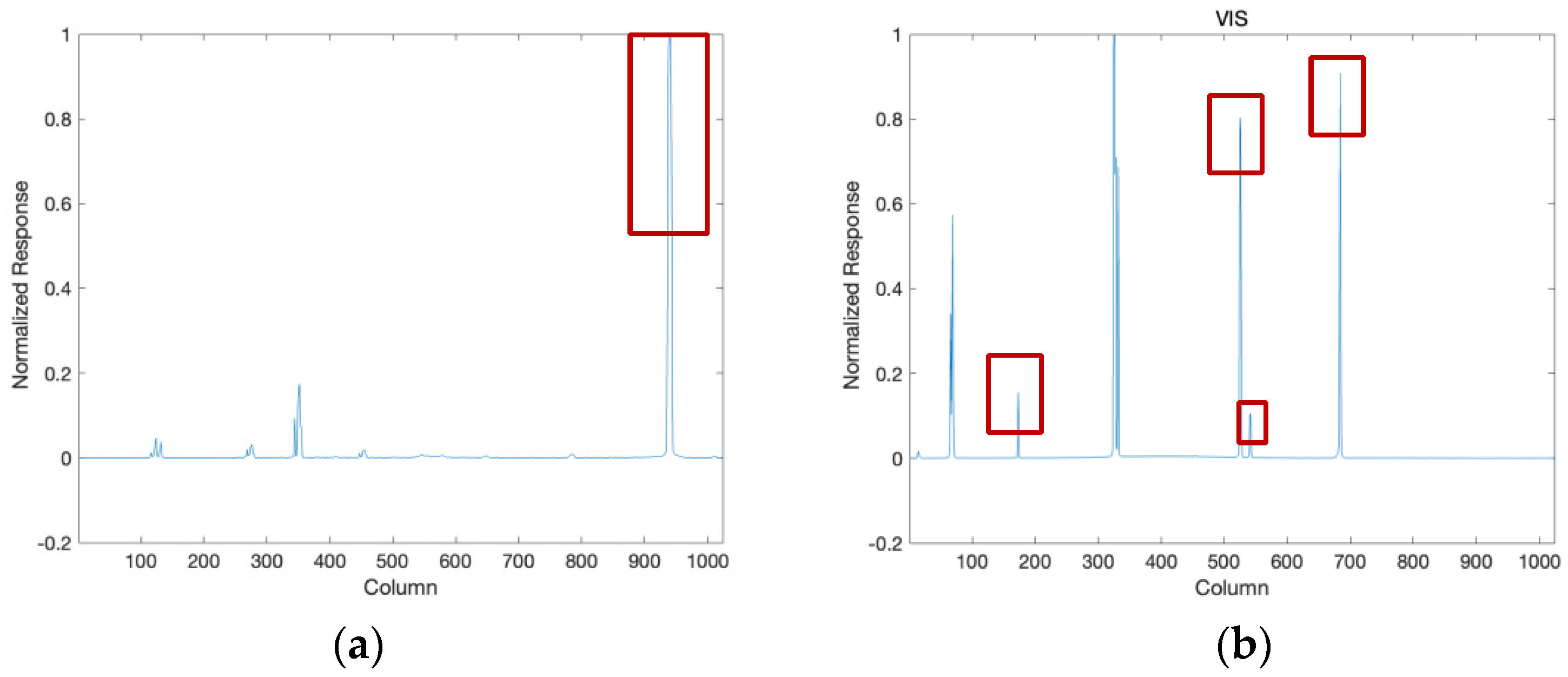
4.5. Analysis of the ISRF in the UV1 Band
4.5.1. The “Secondary Peak” of the ISRF in the UV1 Band
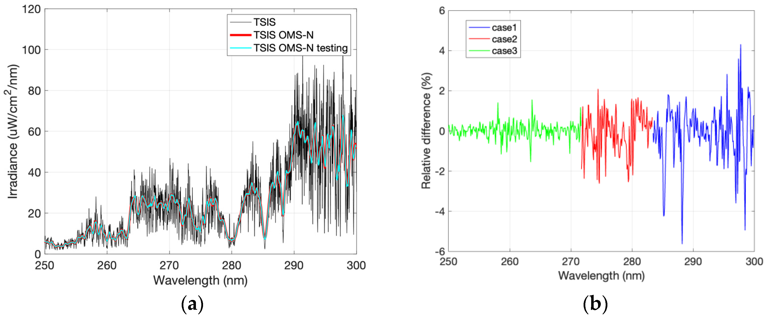
4.5.2. Impact Analysis: Reference Solar Spectra
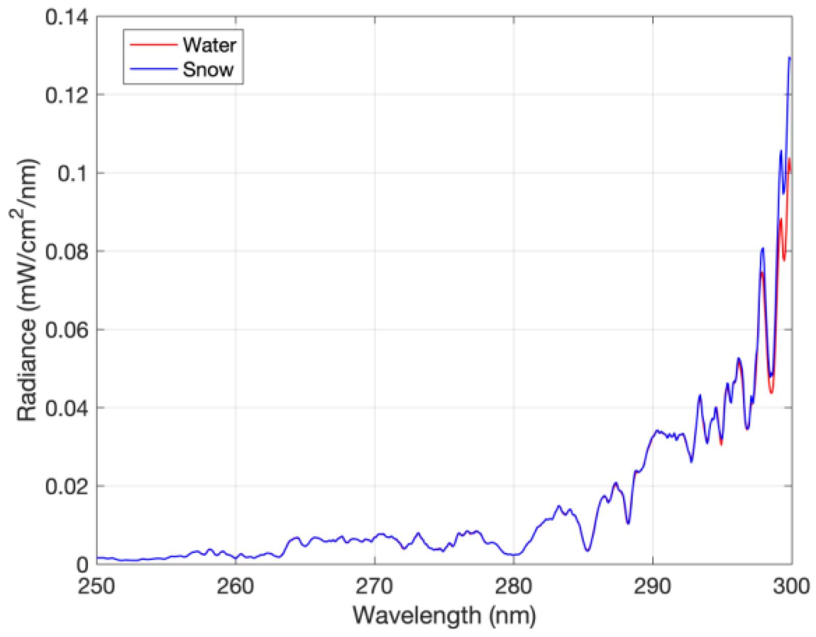
4.5.3. Impact Analysis: Radiative Transfer Model
5. Conclusions
- The spectral resolution and spectral accuracy of OMS-N meet the mission requirements.
- The characterization of the ISRF shows an “asymmetric central peak” and “secondary peak” in the middle–long wavelength, and a slight “asymmetric central peak” in the short wavelength of the UV1 band. Additionally, the ISRF in the UV1 band is asymmetric, which is more noticeable for nadir rows compared with side rows.
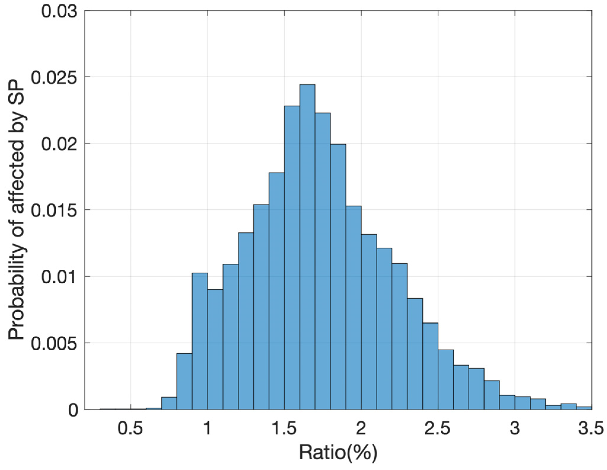
- ISRF characterizations in the UV1 band do not introduce any radiometric systematic bias. However, if the “asymmetric central peak” and “secondary peak” of the ISRF are ignored, they will bring about an error of ± 2% while simulating observation spectra, with an amplified influence on the center of the absorption line. In data application, the measured ISRF instead of the ISRF fitted by the FWHM should be used, which could avoid the larger errors in the center of the absorption line.
Author Contributions
Funding
Data Availability Statement
Acknowledgments
Conflicts of Interest
References
- Aminou, D. Copernicus Sentinels 4 and 5 Mission Requirements Traceability Document. [2022-03-02]. 2017. Available online: https://sentinel.esa.int/documents/247904/0/Copernicus-Sentinels-4-and-5-Mission-Requirements-Traceability-Document.pdf/b15b6786-88cd-4f1d-a67e-a1da70ed595b (accessed on 4 May 2023).
- Ingmann, P.; Veihelmann, B.; Langen, J.; Lamarre, D.; Stark, H.; Courrèges-Lacoste, G.B. Requirements for the GMES Atmosphere Service and ESA’s implementation concept: Sentinels-4/-5 and -5p. Remote Sens. Environ. 2012, 120, 58–69. [Google Scholar] [CrossRef]
- Orfanoz-Cheuquelaf, A.; Rozanov, A.; Weber, M.; Arosio, C.; Ladstätter-Weißenmayer, A.; Burrows, J.P. Total ozone column from Ozone Mapping and Profiler Suite Nadir Mapper (OMPS-NM) measurements using the broadband weighting function fitting approach (WFFA). Atmos. Meas. Tech. 2021, 14, 5771–5789. [Google Scholar] [CrossRef]
- Pan, C.; Weng, F.; Flynn, L. Spectral performance and calibration of the Suomi NPP OMPS Nadir/Profiler sensor. Earth Space Sci. 2017, 4, 737–745. [Google Scholar] [CrossRef]
- Munro, R.; Lang, R.; Klaes, D.; Poli, G.; Retscher, C.; Lindstrot, R.; Huckle, R.; Lacan, A.; Grzegorski, M.; Holdak, A.; et al. The GOME-2 instrument on the Metop series of satellites: Instrument design, calibration, and level 1 data processing—An overview. Atmos. Meas. Tech. 2016, 9, 1279–1301. [Google Scholar] [CrossRef]
- Zhao, M.; Si, F.; Zhou, H. Pre-Launch Radiometric Characterization of EMI-2 on the GaoFen-5 Series of Satellites. Remote Sens. 2021, 13, 2843. [Google Scholar] [CrossRef]
- Kleipool, Q.; Ludewig, A.; Babić, L.; Bartstra, R.; Braak, R.; Dierssen, W.; Dewitte, P.J.; Kenter, P.; Landzaat, R.; Leloux, J.; et al. Pre-launch calibration results of the TROPOMI payload onboard the Sentinel-5 Precursor sat-ellite. Atmos. Meas. Tech. 2018, 11, 6439–6479. [Google Scholar] [CrossRef]
- Platt, U.; Stutz, J. Differential Optical Absorption Spectroscopy (DOAS). In Air Monitoring by Spectroscopic Techniques; Sigrist, M.W., Ed.; Chemical Analysis Series; Springer: Berlin/Heidelberg, Germany, 2008; pp. 135–174. [Google Scholar]
- Lerot, C.; Van Roozendael, M.; Lambert, J.C.; Granville, J.; Van Gent, J.; Loyola, D.; Spurr, R. The GODFIT algorithm: A direct fitting approach to improve the accuracy of total ozone measurements from GOME. Int. J. Remote Sens. 2010, 31, 543–550. [Google Scholar] [CrossRef]
- Lerot, C.; Van Roozendael, M.; Lambert, J.C.; Granville, J.; Van Gent, J.; Loyola, D.; Spurr, R. Sixteen years of GOME/ERS2 total ozone data: The new direct-fitting GOME Data Processor (GDP) Version 5: I. Algorithm Description. J. Geophys. Res. 2012, 117, D03305. [Google Scholar]
- Tilstra, L.G.; van Soest, G.; Stammes, P. Method for in-flight satellite calibration in the ultraviolet using radiative transfer calculations, with application to Scanning Imaging Absorption Spectrometer for Atmospheric Chartography (SCIAMACHY). J. Geophys. Res. Atmos. 2005, 110, D18311. [Google Scholar] [CrossRef]
- Mettig, N.; Weber, M.; Rozanov, A.; Arosio, C.; Burrows, J.P.; Veefkind, P.; Thompson, A.M.; Querel, R.; Leblanc, T.; Godin-Beekmann, S.; et al. Ozone profile retrieval from nadir TROPOMI measurements in the UV range. Atmos. Meas. Tech. 2021, 14, 6057–6082. [Google Scholar] [CrossRef]
- Garane, K.; Koukouli, M.-E.; Verhoelst, T.; Lerot, C.; Heue, K.P.; Fioletov, V.; Balis, D.; Bais, A.; Bazureau, A.; Dehn, A.; et al. TROPOMI/S5P total ozone column data: Global ground-based validation and consistency with other satellite missions. Atmos. Meas. Tech. 2019, 12, 5263–5287. [Google Scholar] [CrossRef]
- Hao, N.; Loyola, D.; Van Roozendael, M.; Lerot, C.; Spurr, R.; Koukouli, M.; Zyrichidou, I.; Inness, A.; Valks, P.; Zimmer, W.; et al. The operational Near-Real-Time Total Ozone Retrieval Algorithm for GOME-2 on MetOp-A & MetOp-B and perspectives for TROPOMI/S5P, ESA ATMOS. In Proceedings of the Quadrennial Ozone Symposium of the International Ozone Commission (IO3C), Edinburgh, UK, 4–9 September 2016. [Google Scholar]
- Jos, H.; Geffen, V.; Roeland, F. Wavelength calibration of spectra measured by the Global Ozone Monitoring Experiment by use of a high-resolution reference spectrum. Appl. Optics 2003, 42, 2739–2753. [Google Scholar]
- Yang, Z.; Zhen, Y.; Yin, Z.; Lin, C.; Bi, Y.; Liu, W.; Wang, Q.; Wang, L.; Gu, S.; Tian, L. Laboratory spectral calibration of the TanSat atmospheric carbon dioxide grating spectrometer. Geosci. Instrum. Methods Data Syst. 2018, 7, 245–252. [Google Scholar] [CrossRef]
- Smorenburg, K.; Dobber, M.R.; Schenkeveld, E.; Vink, R.; Visser, H. Slit function measurement optical stimulus. In Sensors, Systems, and Next-Generation Satellites VI; SPIE: Bellingham, WA, USA, 2003; Volume 4881, pp. 511–520. [Google Scholar]
- Day, J.O.; O’Dell, C.W.; Pollock, R.; Bruegge, C.J.; Rider, D.; Crisp, D.; Miller, C.E. Preflight Spectral Calibration of the Orbiting Carbon Observatory. IEEE Geosci. Remote Sens. 2011, 49, 2793–2801. [Google Scholar] [CrossRef]
- Lee, R.A.M.; O’Dell, C.W.; Wunch, D.; Roehl, C.M.; Osterman, G.B.; Blavier, J.-F.; Rosenberg, R.; Chapsky, L.; Frankenberg, C.; Hunyadi-Lay, S.L.; et al. Preflight Spectral Calibration of the Orbiting Carbon Observatory 2. IEEE Trans. Geosci. Remote Sens. 2017, 55, 2499–2508. [Google Scholar] [CrossRef]
- Gaiser, S.; Aumann, H.; Strow, L.; Hannon, S.; Weiler, M. In-flight spectral calibration of the atmospheric infrared sounder. IEEE Trans. Geosci. Remote Sens. 2003, 41, 287–297. [Google Scholar] [CrossRef]
- Sun, K.; Liu, X.; Nowlan, C.R.; Cai, Z.; Chance, K.; Frankenberg, C.; Lee, R.A.M.; Pollock, R.; Rosenberg, R.; Crisp, D. Characterization of the OCO-2 instrument line shape functions using on-orbit solar measurements. Atmos. Meas. Tech. 2017, 10, 939–953. [Google Scholar] [CrossRef]
- Beirle, S.; Lampel, J.; Lerot, C.; Sihler, H.; Wagner, T. Parameterizing the instrumental spectral response function and its changes by a super-Gaussian and its derivatives. Atmos. Meas. Tech. 2021, 10, 581–598. [Google Scholar] [CrossRef]
- Robertson, J.G. Quantifying Resolving Power in Astronomical Spectra. Publ. Astron. Soc. Aust. 2013, 30, e048. [Google Scholar] [CrossRef]
- Yan, C.S.; Chen, Y.W.; Yang, H.M.; Ahokas, E. Optical spectrum analyzers and typical applications in astronomy and remote sensing. Rev. Sci. Instrum. 2023, 94, 081501. [Google Scholar] [CrossRef]
- Coddington, O.M.; Richard, E.C.; Harber, D.; Pilewskie, P.; Woods, T.N.; Chance, K.; Liu, X.; Sun, K. The TSIS-1 Hybrid Solar Reference Spectrum. Geophys. Res. Lett. 2021, 48, e2020GL091709. [Google Scholar] [CrossRef] [PubMed]
- Mei, L.; Rozanov, V.; Rozanov, A.; Burrows, J.P. SCIATRAN software package (V4.6): Update and further development of aerosol, clouds, surface reflectance databases and models. Geosci. Model Dev. 2023, 16, 1511–1536. [Google Scholar] [CrossRef]
- Wang, Q.; Zhang, P.; Xu, N.; Chen, L.; Wu, R.; Liu, J.; Si, F. An Investigation on Inter-Calibrating EMI/GF-5 with TROPOMI/S5p in Ultraviolet–Visible Spectra. IEEE Trans. Geosci. Remote Sens. 2022, 60, 1–116. [Google Scholar] [CrossRef]
- Ding, S.; Weng, F. Influences of Physical Processes and Parameters on Simulations of TOA Radiance at UV Wavelengths: Implications for Satellite UV Instrument Validation. J. Meteor. Res. 2019, 33, 264–375. [Google Scholar] [CrossRef]


| Parameter | UV1 | UV2 | VIS |
|---|---|---|---|
| Band coverage | 250–300 nm | 300–320 nm | 310–497 nm |
| Spectral resolution | ~1 nm | ~0.5 nm | ~0.5 nm |
| Spectral sampling | ~0.073 nm | ~0.197 nm | |
| Spectral accuracy | 0.05 nm | 0.01 nm | |
| Spatial resolution for nadir point | 21 km × 28 km | 7 km × 7 km | 7 km × 7 km |
| Equator crossing time | 10:00 local solar time | ||
| Field of view | 112° | ||
| Device | Wavelength Accuracy | Band Coverage | Sampling Step Size |
|---|---|---|---|
| M-squared tunable laser | 0.001 nm | 250–300 nm 350–493 nm | 0.05 nm 0.02 nm |
| OPO tunable laser | 0.0001 nm | 300–350 nm | 2 nm |
| Standard spectral lamp | 0.0005 nm | 253.652 nm 334.1484 nm 404.657 nm 407.7837 nm 435.834 nm | - |
| Band | Reference Wavelength (nm) | Wavelength Accuracy (nm) | Requirement (nm) |
|---|---|---|---|
| UV1 | 253.652 | −0.031 | 0.05 |
| VIS | 334.1484 | −0.010 | 0.01 |
| 404.657 | −0.0014 | ||
| 407.7837 | 0.0058 | ||
| 435.834 | −0.0061 |
Disclaimer/Publisher’s Note: The statements, opinions and data contained in all publications are solely those of the individual author(s) and contributor(s) and not of MDPI and/or the editor(s). MDPI and/or the editor(s) disclaim responsibility for any injury to people or property resulting from any ideas, methods, instructions or products referred to in the content. |
© 2024 by the authors. Licensee MDPI, Basel, Switzerland. This article is an open access article distributed under the terms and conditions of the Creative Commons Attribution (CC BY) license (https://creativecommons.org/licenses/by/4.0/).
Share and Cite
Wang, Q.; Wang, Y.; Xu, N.; Mao, J.; Sun, L.; Shi, E.; Hu, X.; Chen, L.; Yang, Z.; Si, F.; et al. Preflight Spectral Calibration of the Ozone Monitoring Suite-Nadir on FengYun 3F Satellite. Remote Sens. 2024, 16, 1538. https://doi.org/10.3390/rs16091538
Wang Q, Wang Y, Xu N, Mao J, Sun L, Shi E, Hu X, Chen L, Yang Z, Si F, et al. Preflight Spectral Calibration of the Ozone Monitoring Suite-Nadir on FengYun 3F Satellite. Remote Sensing. 2024; 16(9):1538. https://doi.org/10.3390/rs16091538
Chicago/Turabian StyleWang, Qian, Yongmei Wang, Na Xu, Jinghua Mao, Ling Sun, Entao Shi, Xiuqing Hu, Lin Chen, Zhongdong Yang, Fuqi Si, and et al. 2024. "Preflight Spectral Calibration of the Ozone Monitoring Suite-Nadir on FengYun 3F Satellite" Remote Sensing 16, no. 9: 1538. https://doi.org/10.3390/rs16091538
APA StyleWang, Q., Wang, Y., Xu, N., Mao, J., Sun, L., Shi, E., Hu, X., Chen, L., Yang, Z., Si, F., Liu, J., & Zhang, P. (2024). Preflight Spectral Calibration of the Ozone Monitoring Suite-Nadir on FengYun 3F Satellite. Remote Sensing, 16(9), 1538. https://doi.org/10.3390/rs16091538